Dynamics of a Small Neutrally Buoyant Sphere in a Fluid and Targeting in Hamiltonian Systems

Abstract

We show that, even in the most favorable case, the motion of a small spherical tracer suspended in a fluid of the same density may differ from the corresponding motion of an ideal passive particle. We demonstrate furthermore how its dynamics may be applied to target trajectories in Hamiltonian systems.

We show with the simplest model for the force acting on a small rigid neutrally buoyant spherical tracer particle in an incompressible two-dimensional fluid flow that tracer trajectories separate from fluid trajectories in those regions where the flow has hyperbolic stagnation points. A tracer will only evolve on fluid trajectories with Lyapunov exponents bounded by the value of its reciprocal Stokes number. By making the Stokes number large enough, one can force a tracer in a flow with chaotic pathlines to settle on either the regular KAM-tori dominated regions or to selectively visit the chaotic regions with small Lyapunov exponents. These findings should be of interest for the interpretation of Lagrangian observations, for example in oceanography, and in laboratory fluid experiments that use small neutrally buoyant tracers. Moreover, since a two-dimensional incompressible flow is a particular instance of a generically chaotic Hamiltonian system, our results constitute a tool for targeting trajectories in Hamiltonian systems.

Our starting point is the equation of motion for a small rigid spherical tracer in an incompressible fluid,

$$\rho_{p}\displaystyle\frac{d{\mathbf{v}}}{dt}= \rho_{f}\displaystyle\frac{D{\mathbf{u}}}{Dt}+(\rho_{p}-\rho_{f}){\mathbf{g}}$$ (4)

$$-\displaystyle\frac{9\nu\rho_{f}}{2a^{2}}\left({\mathbf{v}}-{\mathbf{u}}-\displaystyle\frac{a^{2}}{6}\nabla^{2}{\mathbf{u}}\right)$$

$$-\displaystyle\frac{\rho_{f}}{2}\left(\displaystyle\frac{d{\mathbf{v}}}{dt}-\displaystyle\frac{D}{Dt}\left[{\mathbf{u}}+\displaystyle\frac{a^{2}}{10}\nabla^{2}{\mathbf{u}}\right]\right)$$

$$-\displaystyle\frac{9\rho_{f}}{2a}\displaystyle\sqrt{\frac{\nu}{\pi}}\displaystyle\int_{0}^{t}\displaystyle\frac{1}{\sqrt{t-\zeta}}\displaystyle\frac{d}{d\zeta}\left({\mathbf{v}}-{\mathbf{u}}-\displaystyle\frac{a^{2}}{6}\nabla^{2}{\mathbf{u}}\right)d\zeta,$$

where ${\mathbf{v}}$ represents the velocity of the particle, ${\mathbf{u}}$ that of the fluid, $\rho_{p}$ the density of the particle, $\rho_{f}$, the density of the fluid it displaces, $\nu$, the kinematic viscosity of the fluid, $a$, the radius of the particle, and $\mathbf{g}$, gravity. The terms on the right represent respectively the force exerted by the undisturbed flow on the particle, buoyancy, Stokes drag, the added mass, and the Basset–Boussinesq history force [boussinesq, basset]. The terms in $a^{2}\nabla^{2}{\mathbf{u}}$ are the Faxén corrections [faxen]. The equation is as given by Maxey & Riley [maxey], except for the added mass term, whose correct form was first derived by Taylor [taylor], as was pointed out by Auton et al. [auton]. The derivative $D{\mathbf{u}}/Dt$ is along the path of a fluid element

$$\frac{D{\mathbf{u}}}{Dt}=\frac{\partial{\mathbf{u}}}{\partial t}+({\mathbf{u}}\cdot\nabla){\mathbf{u}},$$ (6)

whereas the derivative $d{\mathbf{u}}/dt$ is taken along the trajectory of the particle

$$\frac{d{\mathbf{u}}}{dt}=\frac{\partial{\mathbf{u}}}{\partial t}+({\mathbf{v}}\cdot\nabla){\mathbf{u}}.$$ (7)

Equation (LABEL:eom) is valid where the particle radius and its Reynolds number are small, as are the velocity gradients around it, and the initial velocities of the particle and the fluid are equal. An excellent review of the history and physics of this problem is provided by Michaelides [michaelides].

We shall simplify Eq. (LABEL:eom) even further with the aim of discovering whether in the most favorable case a tracer particle may always be faithful to a flow trajectory. With this in mind, we set $\rho_{p}=\rho_{f}$, so that the tracer be neutrally buoyant. At the same time we assume that it be sufficiently small that the Faxén corrections be negligible. Furthermore we exclude the Basset–Boussinesq term, since our approach — in which we follow Einstein and others [einstein, russel, crisanti] — is to obtain a minimal model with which we may perform a mathematical analysis of the problem. If in this model there appear differences between particle and flow trajectories, with the inclusion of further terms these discrepancies will remain or may even be enhanced [druzhinin, tanga, yannacopoulos]. If we rescale space, time, and velocity by scale factors $L$, $T=L/U$, and $U$, we arrive at the expression

$$\frac{d{\mathbf{v}}}{dt}=\frac{D{\mathbf{u}}}{Dt}-{\mathrm{S}t}^{-1}\left({\mathbf{v}}-{\mathbf{u}}\right)-\frac{1}{2}\left(\frac{d{\mathbf{v}}}{dt}-\frac{D{\mathbf{u}}}{Dt}\right),$$ (8)

where ${\mathrm{S}t}$ is the particle Stokes number ${\mathrm{S}t}=2a^{2}U/(9\nu L)=2/9\,(a/L)^{2}{\mathrm{R}e}_{f}$, ${\mathrm{R}e}_{f}$ being the fluid Reynolds number. The assumptions involved in deriving Eq. (LABEL:eom) require that ${\mathrm{S}t}\ll 1$.

In the past it has been assumed that sufficiently small neutrally buoyant particles have trivial dynamics [crisanti, druzhinin], and the mathematical argument used to back this up is that if we make the approximation $D{\mathbf{u}}/Dt=d{\mathbf{u}}/dt$, the problem becomes very simple:

$$\frac{d}{dt}({\mathbf{v}}-{\mathbf{u}})=-\frac{2}{3}\,{\mathrm{S}t}^{-1}({\mathbf{v}}-{\mathbf{u}}).$$ (9)

Thence ${\mathbf{v}}-{\mathbf{u}}=\left({\mathbf{v}}_{0}-{\mathbf{u}}_{0}\right)\exp(-2/3\,{\mathrm{S}t}^{-1}\,t)$, from which we infer that even if we release the particle with a different initial velocity ${\mathbf{v}}_{0}$ to that of the fluid ${\mathbf{u}}_{0}$, after a transient phase the particle velocity will match the fluid velocity, $\mathbf{v}=\mathbf{u}$, meaning that following this argument, a neutrally buoyant particle should be an ideal tracer. Although from the foregoing it would seem that neutrally buoyant particles represent a trivial limit to Eq. (LABEL:eom), this would be without taking into account that in a correct approach to the problem $D{\mathbf{u}}/Dt\neq d{\mathbf{u}}/dt$. If we substitute the expressions for these derivatives given in Eqs. (6) and (7) into Eq. (8), we obtain

$$\frac{d}{dt}\left({\mathbf{v}}-{\mathbf{u}}\right)=-\left(\left({\mathbf{v}}-{\mathbf{u}}\right)\cdot\nabla\right){\mathbf{u}}-\frac{2}{3}\,{\mathrm{S}t}^{-1}\left({\mathbf{v}}-{\mathbf{u}}\right).$$ (10)

We may then write ${\mathbf{A}}={\mathbf{v}}-{\mathbf{u}}$, whence

$$\frac{d{\mathbf{A}}}{dt}=-\left(J+\frac{2}{3}\,{\mathrm{S}t}^{-1}I\right)\cdot{\mathbf{A}},$$ (11)

where $J$ is the Jacobian matrix — we shall now concentrate on two-dimensional flows ${\mathbf{u}}=(u_{x},u_{y})$ —

$$J=\left(\begin{array}[]{cc}\partial_{x}u_{x}&\partial_{y}u_{x}\\ \partial_{x}u_{y}&\partial_{y}u_{y}\end{array}\right).$$ (12)

If we diagonalize the matrix we obtain

$$\frac{d{\mathbf{A}}_{D}}{dt}=\left(\begin{array}[]{cc}\lambda-2/3\,{\mathrm{S}t}^{-1}&0\\ 0&-\lambda-2/3\,{\mathrm{S}t}^{-1}\end{array}\right)\cdot{\mathbf{A}}_{D},$$ (13)

so if ${\mbox{\it Re}}(\lambda)>2/3\,{\mathrm{S}t}^{-1}$, ${\mathbf{A}}_{D}$ may grow exponentially. Now $\lambda$ satisfies $\mathrm{det}(J-\lambda I)=0$, so $\lambda^{2}-{\mathrm{t}r}J+{\mathrm{d}et}J=0$. Since the flow is incompressible, $\partial_{x}u_{x}+\partial_{y}u_{y}=\mathrm{tr}J=0$, thence $-\lambda^{2}=\mathrm{det}J$. Given squared vorticity $\omega^{2}=(\partial_{x}u_{y}-\partial_{y}u_{x})^{2}$, and squared strain $s^{2}=s_{1}^{2}+s_{2}^{2}$, where the normal component is $s_{1}=\partial_{x}u_{x}-\partial_{y}u_{y}$ and the shear component is $s_{2}=\partial_{y}u_{x}+\partial_{x}u_{y}$, we may write

$$Q=\lambda^{2}=-{\mathrm{d}et}J=(s^{2}-\omega^{2})/4,$$ (14)

where $Q$ is the Okubo–Weiss parameter [okubo, weiss2]. If $Q>0$, $\lambda^{2}>0$, and $\lambda$ is real, so deformation dominates, as around hyperbolic points, whereas if $Q<0$, $\lambda^{2}<0$, and $\lambda$ is imaginary, so rotation dominates, as near elliptic points. Equation (11) together with $d{\mathbf{x}}/dt={\mathbf{A}}+{\mathbf{u}}$ defines a dissipative dynamical system

$$d\mbox{\boldmath$\xi$}/dt={\mathbf{F}}(\mbox{\boldmath$\xi$})$$ (15)

with constant divergence $\nabla\cdot{\mathbf{F}}=-4/3\,{\mathrm{S}t}^{-1}$ in the four dimensional phase space $\mbox{\boldmath$\xi$}=(x,y,A_{x},A_{y})$, so that while small values of ${\mathrm{S}t}$ allow for large values of the divergence, large values of ${\mathrm{S}t}$ force the divergence to be small. The Stokes number is the relaxation time of the particle back onto the fluid trajectories compared to the time scale of the flow — with larger ${\mathrm{S}t}$, the particle has more independence from the fluid flow. From Eq. (13), about areas of the flow near to hyperbolic stagnation points with $Q>4/9\,{\mathrm{S}t}^{-2}$, particle and flow trajectories separate exponentially.

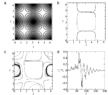
FIG. 1.: (a) Fluid trajectories (thick lines) and magnitude of $Q$ (background shading: lighter is higher $Q$) for the time-independent model Eq. (16) with $A=100$ and $B=0$. The flow is on a torus. (b) Separation of a neutrally buoyant particle trajectory (solid line) with Stokes number ${\mathrm{S}t}=0.2$ from the flow (dashed line) in regions of high $Q$ allows the particle to wander between cells. (c) After a complicated excursion, a particle eventually settles in a zone of low $Q$. (d) The velocity difference $v_{x}-u_{x}$ between the particle and the flow against time for case (c).

To illustrate the effects of ${\mathrm{S}t}$ and $Q$ on the dynamics of a neutrally buoyant particle, let us consider the simple incompressible two-dimensional model flow defined by the stream function

$$\psi(x,y,t)=A\cos(x+B\sin\omega t)\cos y.$$ (16)

The equations of motion for an element of the fluid will then be $\dot{x}=\partial_{y}\psi$, $\dot{y}=-\partial_{x}\psi$. $\psi$ has the rôle of a Hamiltonian for the dynamics of such an element, with $x$ and $y$ playing the parts of the conjugate coordinate and momentum pair. Let us first consider the simplest case where the time dependence is suppressed, by setting $B=0$. Thence $\psi$ should be a constant of motion, which implies that real fluid elements follow trajectories that are level curves of $\psi$. Such level curves are depicted in Fig. 1a, which also shows contours of $Q$. The high values of $Q$ are around the hyperbolic points, while negative $Q$ coincides with the centers of vortices — elliptic points — in the flow. Figure 1b shows the trajectory of a neutrally buoyant particle starting from a point on a fluid trajectory within the central vortex, with an inappreciable velocity mismatch with the flow. This mismatch is amplified in the vicinity of the hyperbolic stagnation points where $Q$ is larger than $4/9\,{\mathrm{S}t}^{-2}$ to the extent that the particle leaves the central vortex for one of its neighbors, a trip that is not allowed to a fluid parcel. In the end a particle settles on a trajectory, proper for a fluid parcel, that does not visit regions of high $Q$. While this effect is already seen in Fig. 1b, it is more dramatically pictured in the trajectory shown in Fig. 1c, in which the particle performs a long and complicated excursion wandering between different vortices before it settles in a region of low $Q$ of one of them. To illustrate the divergence of particle and fluid trajectories, and the fact that particle and fluid finally arrive at an accord, in Fig. 1d we display the difference between the particle velocity and the fluid velocity at the site of the particle against time for the case of Fig. 1c. This difference is initially inappreciable, and it converges to zero at long times, but during the interval in which the excursion takes place it fluctuates wildly.

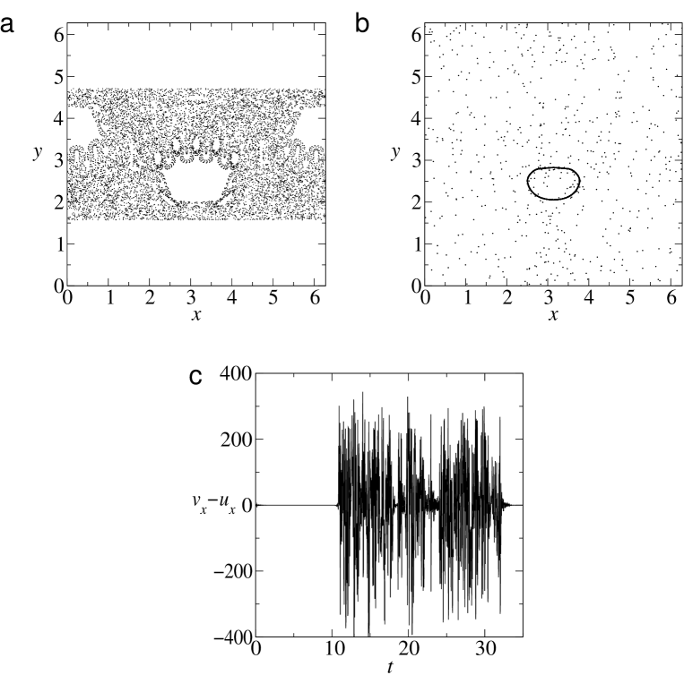
FIG. 2.: Poincaré sections of trajectories in the time-dependent flow of Eq. (16) with $A=250$, $B=0.3$, and $\omega=1.0$. (a) A chaotic fluid trajectory. (b) The motion of a neutrally buoyant particle with Stokes number ${\mathrm{S}t}=0.2$ in the flow. (c) The velocity difference $v_{x}-u_{x}$ between the particle and the flow against time.

Even more interesting is the case of time-dependent flow: $B\neq 0$ in our model. As in a typical Hamiltonian system, associated with the original hyperbolic stagnation points, there are regions of the phase space, which is here real space, dominated by chaotic trajectories. An individual trajectory of this kind, stroboscopically sampled at the frequency of the flow, is reproduced in Fig. 2a. Such a trajectory visits a large region of the space, which includes the original hyperbolic stagnation points and their vicinities where $Q$ is large. Excluded from the reach of such a chaotic trajectory remain areas where the dynamics is regular; the so-called KAM tori. In our model these lie in the regions where $Q<4/9\,{\mathrm{S}t}^{-2}$. Now a neutrally buoyant particle that tries to follow a chaotic flow pathline will eventually reach the highly hyperbolic regions of the flow. This makes likely its separation and departure from such a pathline, in search of another pathline to which to converge. However, convergence will only be achieved if the pathline never crosses areas of high $Q$. Figures 2b and 2c demonstrate this phenomenon: a particle was released in the chaotic zone with an inappreciable velocity mismatch. The particle followed the flow, until, coming upon a region of sufficiently high $Q$, it was thrown out of that flow pathline onto a long excursion that finally ended up in a regular region of the flow on a KAM torus. The regular regions of the flow then constitute attractors of the dissipative dynamical system Eq. (15) that describes the behavior of a neutrally buoyant particle. The chaotic trajectories in a Hamiltonian system are characterized by positive Lyapunov exponents. The Lyapunov exponents are an average along the trajectory of the local rate of convergence or divergence. Such a rate is measured by the quantity $\lambda$. Hence, for a trajectory to be chaotic, it is a necessary condition that it visit regions of positive $Q$: an upper bound to $Q$ is an upper bound to the Lyapunov exponent.

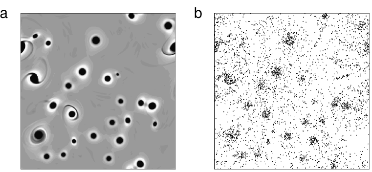
FIG. 3.: Small neutrally buoyant tracer particles with Stokes number ${\mathrm{S}t}=0.2$ collect in the centers of vortices in a two-dimensional turbulent flow simulation. (a) $Q$ field at time $t=1$ (lighter shading is higher $Q$), (b) distribution at time $t=1$ of particles that were uniformly distributed in the flow at time $t=0$.

We have considered the implications of these results for two-dimensional turbulent flows, in which $Q$ defines three regions: in the vortex centers it is strongly negative; in the circulation cells that surround them, strongly positive, while in the background between vortices it fluctuates close to zero [elhmaidi, basdevant, hua, protas, provenzale]. We solve the two-dimensional vorticity equation for an incompressible fluid, $\partial_{t}\omega+J(\omega,\psi)=D_{\omega}$, where $D_{\omega}=-\nu\nabla^{4}\omega$ represents subgrid-scale dissipation; see, e.g., McWilliams [mcwilliams]. We integrate this equation on a doubly periodic domain using a pseudospectral method with $512^{2}$ collocation points and $\nu=2.5\cdot 10^{-7}$; see Montabone [montabone] and Provenzale [provenzale] for details. As a result of the dynamics, an initially uniform distribution of small neutrally buoyant particles evolves in time towards an asymptotic distribution concentrated in the inner part of vortices where $Q<0$, and with voids in the areas crossed by fluid trajectories that visit regions where $Q>4/9\,{\mathrm{S}t}^{-2}$, as we illustrate in Fig. 3. This has importance consequences for the design of both fluid experiments using neutrally buoyant tracer particles, and Lagrangian drifters in geophysical flows.

Now let us consider the following problem in the realm of Hamiltonian dynamics: given a generic chaotic Hamiltonian $H(p_{1},\ldots p_{n},q_{1},\ldots q_{n})$, we might like to find orbits with Lyapunov exponents with a given bound. In particular, we may be interested in locating small KAM tori in a chaotic sea. Inspired by the above results, we may follow the dynamics of a small neutrally buoyant hypersphere in a 2$N$-dimensional hyperfluid. By this, we mean a particle that follows a simplified Maxey–Riley equation, Eq. (8), extended to 2$N$ dimensions, which leads to a generalization of Eq. (15), $d{\mathbf{A}}_{D}/dt=M\cdot{\mathbf{A}}_{D}$, with elements $M_{ij}=\delta_{i,j}[(-1)^{i-1}\lambda_{[(i+1)/2]}-2/3\,{\mathrm{S}t}^{-1}]$, where $[.]$ denotes the integer part, replacing Eq. (13). Thus the Stokes number retains the same control over the Lyapunov exponents as in two dimensions. The quantity $\mathbf{A}$ may be viewed as the control signal: it vanishes when the desired trajectory is reached. In this light, the dynamics of a neutrally buoyant particle as demonstrated above may be thought of as a tool for targeting in Hamiltonian systems.

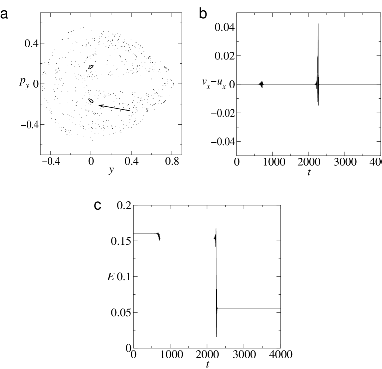
FIG. 4.: (a) A particle in a hyperfluid defined by the Hénon–Heiles Hamiltonian finds a KAM torus (arrowed) in the flow. (b) The velocity difference $A_{x}=v_{x}-u_{x}$ between the particle and the flow against time. (c) The Hénon–Heiles energy $E$ against time.

In Fig. 4 we illustrate our targeting mechanism with the Hénon–Heiles Hamiltonian $H=1/2(x^{2}+y^{2}+p_{x}^{2}+p_{y}^{2})+x^{2}y-y^{3}/3$. Figure 4a shows with a Poincaré section how a particle released into a Hénon–Heiles flow ends up on a KAM torus. In Fig. 4b we plot one component of the velocity difference between particle and flow; it displays two episodes of particle–flow separation before the particle settles on a KAM torus. Since it is not obliged to conserve the Hénon–Heiles energy, the energy at which the particle finally settles into the Hamiltonian flow is a priori undefined; Fig. 4c shows a series of plateaux punctuated by rapid energy jumps correlated with the separations. If one is interested in finding a KAM torus at a given energy, this constraint should be imposed on the dynamics of the particle.

We are grateful to Luca Montabone for Fig. 3, and to Bill Young for useful discussions. JHEC and OP acknowledge the financial support of the Spanish DGICyT, contract PB94-1167, and CICyT contract MAR98-0840. JHEC also thanks the Spanish CSIC for financial support. This work was completed at the European Science Foundation TAO (Transport processes in the Atmosphere and Oceans) Study Centre held in Palma de Mallorca, Spain, during September 1999; we thank the ESF for its support.

REFERENCES

- [1] babiano@ella.ens.fr.
- [2] julyan@galiota.uib.es, WWW http://formentor.uib.es/julyan.
- [3] piro@imedea.uib.es, WWW http://www.imedea.uib.es/piro.
- [4] anto@icg.to.infn.it.