Temporal Modulation of the Control Parameter in Electroconvection in the Nematic Liquid Crystal I52

Abstract

I report on the effects of a periodic modulation of the control parameter on electroconvection in the nematic liquid crystal I52. Without modulation, the primary bifurcation from the uniform state is a direct transition to a state of spatiotemporal chaos. This state is the result of the interaction of four, degenerate traveling modes: right and left zig and zag rolls. Periodic modulations of the driving voltage at approximately twice the traveling frequency are used. For a large enough modulation amplitude, standing waves that consist of only zig or zag rolls are stabilized. The standing waves exhibit regular behavior in space and time. Therefore, modulation of the control parameter represents a method of eliminating spatiotemporal chaos. As the modulation frequency is varied away from twice the traveling frequency, standing waves that are a superposition of zig and zag rolls, i.e. standing rectangles, are observed. These results are compared with existing predictions based on coupled complex Ginzburg-Landau equations.

I Introduction

When a spatially extended system is driven far from equilibrium, a series of transitions occurs as a function of the external driving force, or control parameter [1]. The initial transition is typically from a spatially uniform state to a state with periodic spatial variations, called a pattern. As the control parameter is increased, a sequence of instabilities occurs that produces increasingly complex spatiotemporal patterns. Ultimately, the system becomes fully turbulent. States of spatiotemporal chaos form an interesting class of patterns [1, 2]. Loosely speaking, spatiotemporal chaos refers to deterministic patterns that possess a random variation in space and time. They generally exhibit an underlying periodicity but are characterized by a finite correlation length and correlation time. Since their discovery in fluid dynamical systems [3], states of spatiotemporal chaos have been observed in a wide range of systems, including Rayleigh-Bénard convection, Faraday instabilities, Taylor-Couette flow, electroconvection in nematic liquid crystals, lasers, and chemical reactions [1, 2]. Despite the ubiquitous nature of the phenomenon, a full understanding of spatiotemporal chaos remains one of the outstanding problems in nonlinear dynamics.

One of the challenges facing the study of spatiotemporal chaos is the difficulty associated with characterizing the dynamics [1]. Because the systems are spatially extended, they are inherently high dimensional. This precludes the use of many of the successful techniques developed to study low dimensional chaos in dynamical systems [4]. Also, most examples of spatiotemporal chaos occur at sufficiently large values of the control parameter that weakly nonlinear techniques, such as amplitude equations, are only applicable as phenomological models, if at all. The work reported here uses a state of spatiotemporal chaos that occurs in electroconvection in I52 [5]. In contrast to other systems, this state does occur in the weakly nonlinear regime where quantitative comparison between theory and experiment is possible. A fundamental theory of electroconvection, the WEM model [6, 7], exists and provides the necessary starting point for a quantitative derivation of the relevant amplitude equations [8]. Therefore, this system is an ideal candidate for studying spatiotemporal chaos. However, currently only two of the four necessary amplitude equations have been derived and only qualitative predictions exist [8]. In this work, I use temporal modulation as a probe of the system’s dynamics. This provides both a test of the existing amplitude equation description and a means of guiding future experiments and calculations.

For electroconvection [9, 10], a nematic liquid crystal is placed between two properly treated glass plates so that the director is everywhere parallel to the plates and along a chosen axis. A nematic liquid crystal is a fluid in which the molecules have orientational order, and the director refers to the axis parallel to the average alignment of the molecules [11]. The liquid crystal is doped with ionic impurities, and an ac voltage is applied across the sample using transparent electrodes on the glass plates. Above a critical value of the applied voltage, there exists a transition from uniform conduction to convection rolls, with a corresponding periodic variation of the director and concentration of ionic impurities. Because the system is anisotropic, the patterns can be characterized by the angle $\theta$ between the director and the wavevector of the pattern. Electroconvection in the nematic liquid crystal I52 exhibits a forward, Hopf bifurcation to oblique rolls [5]. A Hopf bifurcation is a transition to a traveling wave pattern, and oblique rolls correspond to patterns where $0^{\circ}<\theta<90^{\circ}$ [9]. At onset, because the director only defines an axis and not a positive direction, states with wavevectors of equal magnitude but with angle s $\theta$ and $\pi-\theta$ are degenerate and referred to as zig and zag rolls, respectively. The state close to onset that is studied here consists of four modes: right- and left-traveling zig and zag rolls [5]. It is the interaction of these four modes that results in spatiotemporal chaos.

Resonant modulation of the control parameter in a system with a Hopf bifurcation is known to stabilize standing waves for large enough modulation strength [12, 13, 14, 15, 16, 17]. However, it has not been applied previously to a state of spatiotemporal chaos. There are three main questions addressed in this work. First, I have made a survey of the range of existence of standing wave patterns and their qualitative features for a reasonable set of values of the applied voltage, applied frequency, the modulation strength, and the modulation frequency. Second, there are three possible standing wave solutions: standing rolls (only zig or zag rolls are present), standing rectangles (superimposed zig and zag rolls with equal amplitude), and standing cross rolls (zig and zag rolls with different amplitudes) [17]. I will show that the standing wave states are generally standing rolls, but that standing rectangles can be observed. Finally, I will demonstrate that the standing roll states are temporally regular and that they eventually become spatially uniform. Therefore, this is an example of the elimination of spatiotemporal chaos and provides an interesting contrast to systems where temporal modulation produces irregular behavior in an otherwise regular system [15, 18].

The rest of the paper is organized as follows. Section II provides the details of the experimental techniques. Section III presents the experimental results. In this section, I will report separately on the results of applying modulations of the control parameter below and above the critical voltage for the onset of convection in the absence of modulations. Section IV will discuss the relationship between these results and existing predictions of relevant amplitude equations.

II Experimental details

The experiments were carried out using two electroconvection cells containing the liquid crystal I52 [19]. The first cell was a custom made cell with a thickness of 25 ${\rm\mu m}$. It was formed from two glass slides that were coated with a layer of indium-tin oxide (ITO), a transparent conductor. The conductive coating was etched to form a 0.5 cm x 0.5 cm square electrode in the center of a 2.5 cm x 2.5 cm cell. The director was aligned using a rubbed polyimide. The second cell was a commercial cell obtained from EHC, LTD. [20]. This cell had a thickness of 23 ${\rm\mu m}$. The electrode was a 1.0 cm x 1.0 cm area of ITO in a 2.5 cm x 2.5 cm cell. The alignment was also due to a rubbed polyimide coating. For both cells, there was some forcing of a pattern due to fringing fields at the edge of the electrodes. However, a region existed in the middle of each cell where convection started spontaneously. All measurements were made in this region of the cell to minimize boundary effects.

The main differences between the two samples were the values of the critical voltage and the Hopf frequency due to differences in iodine doping. The custom sample was filled with I52 that had been doped with $6.3\%$ by weight molecular ${\rm I_{2}}$ two months prior to filling the cell. The commercial cell was filled with I52 that had been doped with $6\%$ by weight molecular ${\rm I_{2}}$ seventeen months prior to filling. The custom cell was aged for five months after filling before experiments were started, and the commercial cell was aged for one month after filling. For the custom cell, the critical voltage was approximately 21 V and the Hopf frequency was approximately 0.125 Hz at an applied frequency of 25 Hz. For the commercial cell, the critical voltage was approximately 15 V and the Hopf frequency was approximately 0.34 Hz at an applied frequency of 25 Hz.

It is known for electroconvection in I52 that the level of iodine in the sample will drift in time. This results in drifts in the critical voltage and the Hopf frequency. Because of this drift, the following protocols were used. The critical voltage and Hopf frequency were measured before and after every set of measurements. The modulated voltage had the following form: $V(t)=[V_{o}+V_{m}cos(\omega_{m}t)]cos(\Omega t)$. The two main dimensionless control parameters are: $\epsilon=V_{o}^{2}/V_{c}^{2}-1$ and $b=V_{m}/V_{c}$. Here $V_{c}$ is the critical voltage for the onset of convection in the absence of modulation. The drift in $V_{c}$ was linear in time and corresponded to a drift in $\epsilon$ of 0.001/Hr. This drift is accounted for in all reported values of $b$ and $\epsilon$. The modulation frequency will be discussed in terms of the shift from resonance $(f^{*}-f_{m}/2)$, where $f_{m}$ is the modulation frequency and $f^{*}$ is the natural frequency of the pattern. For $\epsilon<0$, $f^{*}$ is the Hopf frequency $f_{h}$, and for $\epsilon>0$, it is the frequency of the pattern in the absence of modulation. Despite the differences between the two cells and the drift in time of $V_{c}$, the behavior as a function of $b$, $\epsilon$, and $(f^{*}-f_{m}/2)$ is completely reproducible. The sample temperature was held constant at either $40\pm 0.002\ ^{\circ}{\rm C}$ or $42\pm 0.002\ ^{\circ}{\rm C}$. The later temperature was used after the total drift in $V_{c}$ at $40^{\circ}{\rm C}$ had exceeded approximately one volt.

Images were taken using a standard shadowgraph method [21] and are presented here with the undistorted director aligned in the horizontal direction. Because of the well-known nonlinear effects of the shadowgraph method [21], the images have been Fourier filtered so that only the fundamental modes are present. This is essential for highlighting the standing wave character of the modulated pattern.

The frequency of the pattern was determined by taking the Fourier transform of a time series of 32 images. The images typically covered a spatial area containing 18 rolls, though smaller regions of only 7 rolls were also used. The time between images was chosen so that the time series covered 4 to 6 periods of the fundamental frequency.

For the measurements of the dynamics of the local amplitude of each mode, a time series of 32 images was used. The time between images was chosen so that the series consisted of four cycles of the pattern. Each image covered a spatial area of approximately 7 wavelengths. The modulus squared of the space-time Fourier transform of the series, $S({\bf k},\omega)$, was used to compute the amplitude of each mode. The power in each mode, right- and left-traveling zig and zag rolls, was determined by summing $S({\bf k},\omega)$ over a 5 by 5 pixel grid in wavenumber space and 5 pixel window in frequency space. The grid and window were centered on the peak in $S({\bf k},\omega)$ that corresponded to the mode of interest. The amplitude of each mode is the square root of the power.

For measurements of the onset of standing waves, $\epsilon$ was fixed and the value of $b$ was either stepped up or down in increments of 0.005. At each step, the system was equilibrated for 10 minutes before a time series of images was taken. The time series of images were used to determine if the pattern was frequency locked to the modulation and whether or not a standing wave had been established.

III Experimental results

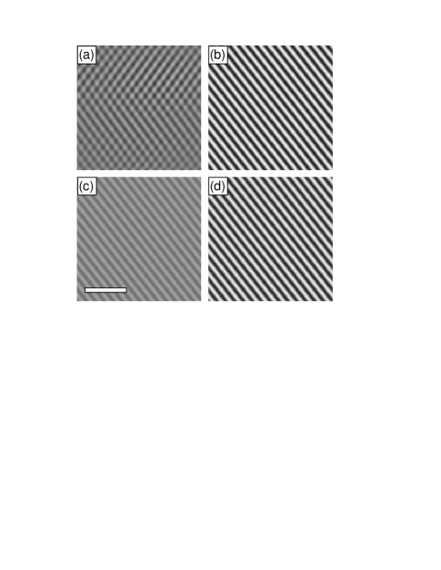
FIG. 1.: Four images of the pattern in a 0.6 mm x 0.6 mm region of the cell. The bar in (c) represent 0.2 mm. (a) An image of the cell at $\epsilon=0.03$ and no modulation. The image has been Fourier filtered so that only the fundamental mode remains. Image (b) through (d) are three images from a time series taken at $\epsilon=0.036$ and $b=0.04$. The images are 0.9 s apart and have also been Fourier filtered. The modulation frequency was 0.694 Hz, which corresponds to twice the Hopf frequency. These images illustrate the standing wave nature of the pattern.

Figure 1 is a comparison of the typical pattern in the region where spatiotemporal chaos exists and the standing wave pattern that is stabilized by the modulation. Figure 1a is a single snapshot of the state of spatiotemporal chaos at a value of $\epsilon=0.03$ and no modulation. Figures 1b-d are three images taken 0.9 s apart of the standing wave state at an $\epsilon=0.036$, $b=0.04$, and $f_{m}=2f_{h}$. The time between the images was chosen to highlight the relative change in phase that is characteristic of a standing wave as one crosses the minimum in intensity. For example, the intensities in the lower right corner in Fig. 1b are opposite those in Fig. 1d.

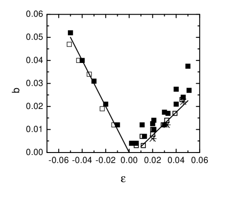
FIG. 2.: The symbols give the location of the transition to standing waves as a function of modulation strength $b$ and reduced control parameter $\epsilon$. The solid symbols and $\times$’s are for increasing the value of $b$. The open symbols and the $+$’s are for decreasing the value of $b$. The difference between the symbols is described in the text. For $\epsilon<0$, there is no pattern present below the symbols, and a spatially uniform pattern exists above the symbols. For $\epsilon>0$, the state of spatiotemporal chaos exists below the symbols. Above the symbols, the system is phase locked to the modulation, and a state of standing rolls exists. For negative $\epsilon$, the solid line is the expected onset based on coupled complex Ginzburg-Landau equations, $b=\epsilon$. For positive $\epsilon$, the solid line is the curve $b=0.57\epsilon-0.006$ and provides a guide to the eye for the transition values.

Figure 2 summarizes the range of existence of the standing wave patterns when a modulation of twice the Hopf frequency is used. The solid symbols and $\times$’s are the location of the transition to standing waves as measured by increasing $\epsilon$. The open symbols and the $+$’s are the location of the transition to standing waves as measured by decreasing $\epsilon$. In the region above and between the two solid lines, the pattern is composed of uniform standing rolls. As a check on the stability of the standing rolls, two runs were made at fixed $b$. For these runs, $\epsilon$ was increased in steps of 0.005, with a waiting time of 5 minutes per step. One run was at $b=0.02$, and the other was at $b=0.05$. For the entire range of $\epsilon$ within the boundaries, only uniform standing rolls were observed at these two values of $b$.

For negative values of $\epsilon$, the behavior of the system is straightforward. The system makes a transition directly from a uniform state to a state of frequency locked standing waves. The pattern consists of either standing zig rolls or standing zag rolls, and never the superposition. The pattern is also frequency locked to half the modulation frequency. As shown in Fig. 2, within the resolution used here, there is essentially no hysteresis in the transition.

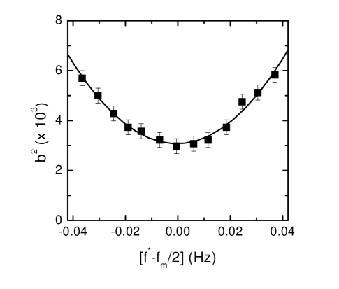
FIG. 3.: Transition to standing waves for $\epsilon=-0.054$. Below the curve, the system is uniform. Above the curve, the state of the system is standing rolls. The symbols are the experimental values. The solid line is a fit to the expected curve: $b^{2}=\epsilon^{2}+(2\pi\tau_{d})^{2}(f^{*}-f_{m}/2)^{2}$. In this case, $f^{*}=0.162$, which is the Hopf frequency of the system.

Figure 3 shows the behavior of the system when the modulation frequency is varied away from twice the Hopf frequency at negative $\epsilon$. The solid squares represent the onset to standing waves, and the solid line is a fit to a parabola. In this case, the parabola is centered on the Hopf frequency.

For positive values of $\epsilon$, the situation is more complicated because the ground state is the state of spatiotemporal chaos. In this case, I have measured the transition in two different ways. First, I have considered the onset to standing rolls. These are the solid and open squares in Fig. 2. When stepping down in $\epsilon$, the transition from standing rolls to the disordered state was easily identified. However, because of the spatial disorder, when $\epsilon$ is increased, the onset to spatially uniform standing rolls is less well-defined. For the purposes of Fig. 2, the onset was taken to be the point where the patches of standing rolls had a size on the order of 18 wavelengths.

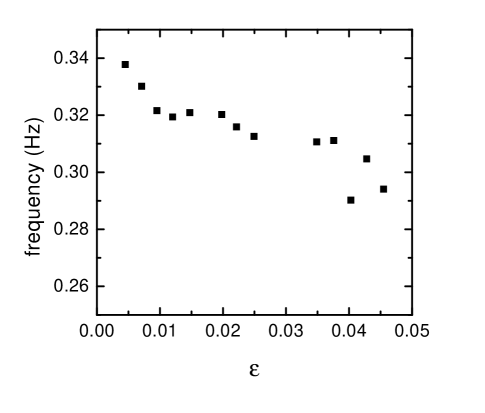
FIG. 4.: Measured frequency of the pattern as a function of $\epsilon$. Illustrates the decrease in the pattern frequency with increasing $\epsilon$.

A better measure of the transition for positive $\epsilon$ is to use the point at which the pattern becomes frequency locked to the modulation frequency. This boundary is given by the $\times$’s and the $+$’s in Fig. 2. Figure 4 shows the plot of the pattern frequency as a function of $\epsilon$ in the absence of modulation. From this, one can see that it is easy to distinguished the locked and unlocked patterns for $\epsilon>0.01$, as the frequency of the pattern differs significantly from the Hopf frequency. With this definition of the transition, there is no measurable hysteresis.

Figure 5 shows the effect of varying the modulation frequency for positive $\epsilon$. As with negative $\epsilon$, the solid line is a fit to a parabola. In this case, the parabola is centered on the frequency of the unmodulated pattern, not the Hopf frequency. Also, when $(f^{*}-f_{m}/2)>0.04$, the standing wave pattern at onset is standing squares. This is illustrated in Fig. 6. For these images, the modulation frequency was 0.472 Hz, and the unmodulated pattern had a frequency of 0.305 Hz. In this range of $(f^{*}-f_{m}/2)$, increasing $b$ leads to a secondary transition from the standing rectangles to standing rolls.

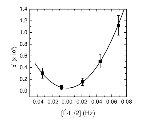
FIG. 5.: Transition to standing waves for $\epsilon=0.03$. Below the curve, the system exhibits spatiotemporal chaos. Above the curve, the system is phase locked to the modulation frequency. The symbols are the experimental values. The solid line is a fit to: $b^{2}=a+b(f^{*}-f_{m}/2)^{2}$. In this case, $f^{*}=0.305~{}Hz$, which is the frequency of the pattern at $\epsilon=0.03$. In contrast, the Hopf frequency is 0.34 Hz. For $|f^{*}-f_{m}/2|<0.04$, the transition is directly to standing rolls. For $(f^{*}-f_{m}/2)>0.04$, the transition is initially to standing rectangles, and there is a secondary transition to standing rolls.

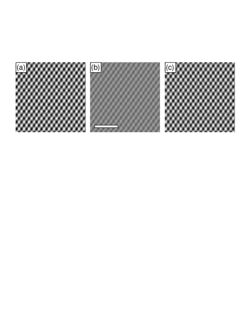
FIG. 6.: Three images from a time series taken at $\epsilon=0.036$, $b=0.04$, and $f_{m}=0.472$. This corresponds to $(f^{*}-f_{m}/2)=0.069$ in Fig. 5. The images cover a region that is 0.6 mm x 0.6 mm and are 0.9 s apart. The bar in (b) represents 0.2 mm. The images have been Fourier filtered so that only the fundamental mode is present. These images illustrate the standing wave nature of the pattern.

I made a qualitative survey of the behavior as a function of the driving frequency. By increasing the driving frequency, one decreases the angle $\theta$ between the wavevector of the pattern and the undistorted director orientation. For our system, the same qualitative behavior was observed for applied frequencies up to 80 Hz. For 80 Hz, $\theta=10^{\circ}$. For modulation at twice the Hopf frequency, a standing roll pattern is observed. A more detailed study of the effects of varying $\theta$ will be the subject of future work.

The local temporal behavior of the standing roll state is extremely regular. This is shown in Fig. 7. Each plot is a time series of the local amplitude. The amplitude is measured every 2 minutes, with the initial point of the time series taken 10 minutes after the modulation is applied. Figure 7a is a plot of the local amplitude as a function of time for $\epsilon=0.01$ and no modulation. The amplitudes of the right-traveling zig rolls, left-traveling zig rolls, and left-traveling zag rolls have been shifted from their true values by 0.015, 0.01, and -0.005, respectively. These shifts clarify the anti-correlations present between the various modes and the irregular variation in time. This behavior has been reported previously [5]. Figure 7b is the local amplitude for $\epsilon=0.01$, $b=0.02$, and $f_{m}=2f_{h}$. This figure shows both the regular temporal behavior and the establishment of standing rolls (the zag amplitude has gone to zero).

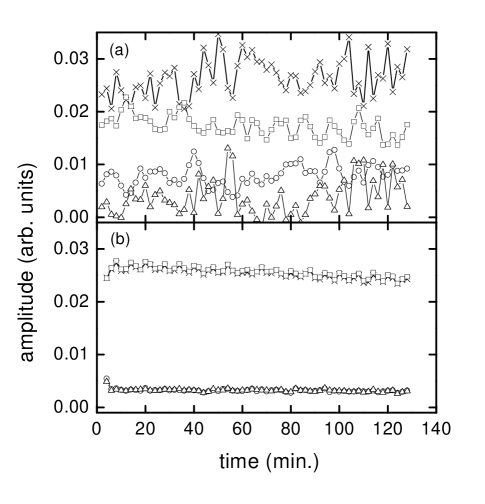
FIG. 7.: (a) Plot of the amplitudes of the right-traveling zig rolls ($\times$), left-traveling zig rolls ($\Box$), right-traveling zag rolls ($\circ$), and left-traveling zag rolls ($\triangle$). The system was at $\epsilon=0.01$ and $b=0\%$. The amplitudes have been shifted as described in the text. (b) Plot of the amplitudes of the right-traveling zig rolls ($\times$), left-traveling zig rolls ($\Box$), right-traveling zag rolls ($\circ$), and left-traveling zag rolls ($\triangle$). The system was at $\epsilon=0.01$ and $b=2.0\%$.

The development of the local, temporal order, generally occurred in under a few minutes. In contrast, the spatial ordering involves extremely long time scales. It can take up to two hours for the standing roll domains to reach sizes on order of the system size. However, upon removal of the modulation, the disorder develops in a few minutes. This difference in time scales is reflected in Fig. 2. One sees that there is essentially no difference between the transition to a frequency locked state and the transition to standing waves measured by decreasing $\epsilon$. However, standing rolls of a particular size occurred at values of $b$ slightly above the transition defined by frequency locking. This is easily understood in terms of the 10 minute waiting time used when stepping $b$. Clearly, the details of the spatial ordering and the multiple time scales involved is an interesting problem. However, it is outside the scope of this paper and will be the subject of future work.

IV Discussion

The transitions for negative $\epsilon$ can be directly compared with predictions of the relevant coupled amplitude equations [17]. I find excellent agreement between the measured onset of standing waves and the predictions of Ref. [17]. The onset to standing waves should occur when $b=|\mu|$. Here the real part of $\mu$ is just $\epsilon$ and the imaginary part of $\mu$ is $2\pi\tau_{d}(f^{*}-f_{m}/2)$, where $\tau_{d}=\gamma_{1}d^{2}/(\pi^{2}K_{11})$ is the director relaxation time. Here $\gamma_{1}$ is a rotational viscosity and $K_{11}$ is the splay elastic constant of the director. For a modulation frequency equal to twice the Hopf frequency, the onset is given by the line $b=\epsilon$. This is the solid line shown in Fig. 1. For the more general case, one has $b^{2}=\epsilon^{2}+(2\pi\tau_{d})^{2}(f_{h}-f_{m}/2)^{2}$. The solid line in Fig. 3 is a fit to this equation. The resulting values are: $\epsilon=-0.058\pm 0.005$, $\tau_{d}=0.229\pm 0.004\ {\rm s}$, and $f_{h}=0.162\pm 0.01\ {\rm Hz}$. For comparison, the measured values of these parameters are: $\epsilon=-0.054\pm 0.002$, $\tau_{d}=0.18\pm 0.05\ {\rm s}$, and $f_{h}=0.164\pm 0.005\ {\rm Hz}$.

The nature of the standing wave pattern depends on the nonlinear coefficients in the amplitude equations. The fact that I observe standing rolls at onset has important consequences. First, the coupling coefficient between zig and zag rolls traveling in the same direction has been calculated [8]. Based on this calculation, it is likely that standing rectangles are the stable state for the parameter range in my experiments. However, the condition for the stability of standing rolls does involve all of the nonlinear coefficients [17], and standing rolls are not ruled out by the calculations of Ref. [8]. Therefore, these experiments highlight the need for a determination of all of the nonlinear coefficients before quantitative comparisons between amplitude equations and the experiments are possible. On the other hand, in the absence of theoretical calculations, the temporal modulation experiments provide a means to determine the coefficients experimentally,

The results for positive $\epsilon$ are in qualitative agreement with the predictions of Ref. [17]. The critical value of $b$ for the transition to standing waves is linear in $\epsilon$ for fixed $f_{m}$. However, I find $b=0.577\epsilon-0.006$ (the solid line in Fig. 2), and not $b=\epsilon$. This is not surprising given that the ground state of the experimental system is a state of spatiotemporal chaos. This pattern can only be described by amplitude equations that include spatial derivatives, and these are not included in Ref. [17]

The other qualitative agreement with Ref. [17] is the behavior as a function of modulation frequency. The critical values of $b^{2}$ are quadratic in $(f^{*}-f_{m}/2)$ for fixed $\epsilon$. However, it is clear from Fig. 5 that $f^{*}$ is the frequency of the unmodulated pattern for the fixed value of $\epsilon$, and not the Hopf frequency. This is due to the shift in frequency with $\epsilon$ that is illustrated in Fig. 4.

An additional feature of the behavior at positive $\epsilon$ that requires a theoretical explanation is the regular dynamics of the standing wave state. Though an incomplete description, the existing amplitude equation calculations suggest that the unmodulated state is Benjamin-Feir unstable for all wavenumbers [8]. This provides a possible explanation for the spatiotemporal chaos at onset. From the fact that the modulated state exhibits regular dynamics, one can infer that the standing rolls are Benjamin-Feir stable. This situation is the opposite of that previously observed in electroconvection in a different nematic liquid crystal [15]. In that system, the unmodulated state was stable. For high enough modulation, the modulated state was Benjamin-Feir unstable and resulted in irregular dynamics [15]. The behavior in that case agreed well with calculations based on amplitude equations that included the spatial derivatives[22]. A similar calculation is needed for the system reported on here. In particular, it will be important to determine if temporal modulation is a general method for eliminating spatiotemporal chaos, or if it is specific to this system.

- [1] For reviews of pattern formation, see M. C. Cross and P. C. Hohenberg, Rev. Mod. Phys. 65, 851 (1993), and J. P. Gollub and J. S. Langer, Rev. Mod. Phys. 71, s396 (1999).
- [2] For a recent review of experiments, see G. Ahlers, Physica A 249, 18 (1998).
- [3] G. Ahlers, Phys. Rev. Lett. 33, 1185 (1974); J. P. Gollub and H. L. Swinney, Phys. Rev. Lett. 35, 927 (1975).
- [4] There are currently many books on this subject. See for instance, K. T. Alligood, T. D. Saver, and J. A. York, Chaos: an introduction to dynamical systems (Springer, New York, 1997).
- [5] M. Dennin, G. Ahlers, and D. S. Cannell, Science 272, 388 (1996).
- [6] M. Treiber and L. Kramer, Mol. Cryst. Liq. Cryst. 261, 311 (1995).
- [7] M. Dennin, M. Treiber, L. Kramer, G. Ahlers, and D. S. Cannell, Phys. Rev. Lett. 76, 319 (1996).
- [8] M. Treiber and L. Kramer, Phys. Rev. E 58, (1998).
- [9] E. Bodenschatz, W. Zimmermann, and L. Kramer, J. Phys. (France) 49, 1875 (1988); L. Kramer, E. Bodenschatz, W. Pesch, W. Thom and W. Zimmermann, Liquid Cryst. 5, 699 (1989).
- [10] Review articles on electroconvection can be found in I. Rehberg, B. L. Winkler, M. de la Torre Juárez, S. Rasenat, and W. Schöpf, Festkörperprobleme 29, 35 (1989); S. Kai and W. Zimmermann, Prog. Theor. Phys. Suppl. 99, 458 (1989); and L. Kramer and W. Pesch, Annu. Rev. Fluid Mec. 27, 515 (1995).
- [11] P. G. de Gennes, The Physics of Liquid Crystals (Claredon Press, Oxford, 1974); S. Chandrasekhar, Liquid Crystals (Cambridge University Press, Cambridge, England, 1992).
- [12] H. Riecke, J. D. Crawford, and E. Knobloch, Phys. Rev. Lett. 61, 1942 (1988).
- [13] D. Walgraef, Europhys. Lett. 7, 485 (1988).
- [14] I. Rehberg, S. Rasenat, J. Fineberg, M. de la Torre Juáurez, and V. Steinberg, Phys. Rev. Lett. 61, 2449 (1988).
- [15] M. de la Torre Juáurez, W. Zimmermann, and I. Rehberg, in Nonlinear Evolution of Spatio-Temporal Structures in Dissipative Continuous Systems, F. H. Busse and L. Kramer, eds., NATO ASI Series B: Physics Vol. 225 (Plenum Press, New York, 1990).
- [16] M. de la Torre Juáurez and I. Rehberg, Phys. Rev. A 42, 2096 (1990).
- [17] H. Riecke, M. Silber, and L. Kramer, Phys. Rev. E 49, 4100 (1994).
- [18] J. P. Gollub and S. V. Benson, Phys. Rev. Lett. 41, 948 (1978).
- [19] U. Finkenzeller, T. Geelhaar, G. Weber, and L. Pohl, Liquid Crystals 5, 313 (1989).
- [20] E.H.C. CO., Ltd., 1164 Hino, Hino-shi, Tokyo, Japan.
- [21] S. Rasenat, G. Hartung, B. L. Winkler, and I. Rehberg, Experiments in Fluids 7, 412 (1989).
- [22] S. Fauve, in Instabilities and Nonequilibrium Structures D. Tirapegui, ed., (D. Reidel Publishing Company, 1987)