Fractal Dimensions of the Hydrodynamic Modes of Diffusion

Abstract.

We consider the time-dependent statistical distributions of diffusive processes in relaxation to a stationary state for simple, two dimensional chaotic models based upon random walks on a line. We show that the cumulative functions of the hydrodynamic modes of diffusion form fractal curves in the complex plane, with a Hausdorff dimension larger than one. In the limit of vanishing wavenumber, we derive a simple expression of the diffusion coefficient in terms of this Hausdorff dimension and the positive Lyapunov exponent of the chaotic model.

1. Introduction

The statistical mechanics of nonequilibrium processes has been the subject of renewed attention. Computer studies have shown that the classical motions of systems with large numbers of particles are typically chaotic [8, 11, 14, 16, 23, 35, 37, 46, 47, 48]. These observations have motivated the theoretical study of low-dimensional model systems where one can obtain quantitative information about nonequilibrium processes in terms of the chaotic properties of the microscopic dynamics of the systems.

In this context, several relationships have been established between transport properties such as diffusion or viscosity and characteristic quantities of chaos such as Lyapunov exponents, Kolmogorov-Sinai (KS) entropy per unit time, and fractal dimensions [1, 4, 5, 10, 15, 17, 19]. These relationships have been obtained for two different types of dynamical systems: (a) deterministic systems with Gaussian thermostats and, (b) open Hamiltonian systems with absorbing boundaries.

In the deterministic systems with Gaussian thermostats [14, 29], the forces ruling the motion of the particles are modified in order to mimic a heat pump removing the excess energy introduced by the external fields or other nonequilibrium constraints. The modified dynamical system is still time-reversal symmetric but volumes are no longer preserved in phase space so that trajectories, in general, converge toward a fractal attractor which has an invariant Sinai-Ruelle-Bowen (SRB) measure, absolutely continuous with respect to Lebesgue measure in unstable directions and fractal in stable directions. On average, the phase-space volumes contract at a rate which increases with the external fields and, thus, with the dissipation of heat. Since the overall contraction rate is equal to the sum of all the Lyapunov exponents, the dissipation turns out to be related to the characteristic quantities of chaos. In this way, formulae have been obtained for the viscosity of an externally sheared fluid [15] and also for the diffusion of a Gaussian-thermostated Lorentz gas [1]. In this last case, the formula relating the diffusion coefficient to the sum of the Lyapunov exponents was also rigorously proved [4, 5]. In the thermostated Lorentz gas, the kinetic energy is constant (instead of the total energy) and the phase space of the flow has thus the dimension three. The Lyapunov exponents of this system are $\lambda^{+}>0>\lambda^{-}$ with $|\lambda^{-}|>\lambda^{+}$ for a nonvanishing field force $F$. In the three-dimensional phase space, the fractal attractor ${\mathcal{A}}_{F}$ has a KS entropy equal to the positive Lyapunov exponent $h_{\rm KS}=\lambda^{+}$ according to Pesin’s equality, and its information dimension is given by Young’s formula: $D_{\rm I}=2+h_{\rm KS}/|\lambda^{-}|$. In this expression for the fractal dimension, the 2 stands for the integer dimensions of the flow direction and of the unstable direction which both are equal to one for the attractor of a flow. However, the attractor is fractal in the stable direction which contributes its partial information dimension $d_{\rm I}=h_{\rm KS}/|\lambda^{-}|$ to the total information dimension of the attractor ${\mathcal{A}}_{F}$. The diffusion coefficient of the Gaussian-thermostated Lorentz gas at temperature $T$ has been alternatively expressed as

$${\mathcal{D}} = \lim_{F\to 0}\left(\frac{k_{\rm B}T}{F}\right)^{2}\ \left[-\lambda^{-}({\mathcal{A}}_{F})-\lambda^{+}({\mathcal{A}}_{F})\right]$$ (1)

$$= \lim_{F\to 0}\left(\frac{k_{\rm B}T}{F}\right)^{2}\ \left[|\lambda^{-}({\mathcal{A}}_{F})|-h_{\rm KS}({\mathcal{A}}_{F})\right]$$

$$= \lim_{F\to 0}\left(\frac{k_{\rm B}T}{F}\right)^{2}\ \lambda^{+}({\mathcal{A}}_{F})\ c_{\rm I}({\mathcal{A}}_{F})\;,$$

where the first form is a consequence of the average contraction of phase-space volumes due to the Gaussian thermostatting mechanism and the relation between the rate of contraction and the rate of entropy production in systems with Gaussian thermostats, the second form follows from the first one by Pesin’s equality, and the third one is obtained by Young formula for the partial information codimension $c_{\rm I}=1-d_{\rm I}=1-h_{\rm KS}/|\lambda^{-}|$ and from the fact that $\lim_{F\to 0}|\lambda^{-}({\mathcal{A}}_{F})|=\lim_{F\to 0}\lambda^{+}({\mathcal{A}}_{F})$ [1, 4, 5, 9]. In the limit of arbitrarily small external field $F$, the information dimension of the fractal attractor approaches the phase-space dimension in a way controlled by the diffusion coefficient, which is the basis of this kind of formulae.

Very similar formulae have been obtained for open Hamiltonian systems with absorbing boundaries [10, 17, 19]. Such boundaries are naturally introduced in systems of scattering type in which particles or trajectories undergo transient collisions before escaping out of a phase-space region of varying geometry. The absorbing boundaries have the effect of driving the system out of equilibrium without a modification of the forces which can remain Hamiltonian, i.e., time-reversal symmetric and also volume preserving. The escape of trajectories leads to the formation of a fractal repeller, described by a invariant Gibbs measure which is fractal in both the unstable and the stable directions. For such systems, the rate of escape is given as the difference between the sum of positive Lyapunov exponents and the KS entropy [12, 30], calculated with respect to the invariant Gibbs measure on the repeller. This escape-rate formula was rigorously proved for Anosov maps with rectangular holes [6, 7]. For the conservative Lorentz gas with absorbing boundaries separated by a distance $L$, the Lyapunov exponents are $\lambda^{+}>0>\lambda^{-}=-\lambda^{+}$ and the diffusion coefficient has been obtained by the following formulae [17, 19] where the quantities are evaluated for the fractal repeller ${\mathcal{R}}_{L}$:

$${\mathcal{D}} = \lim_{L\to\infty}\left(\frac{L}{\pi}\right)^{2}\ \left[\lambda^{+}({\mathcal{R}}_{L})-h_{\rm KS}({\mathcal{R}}_{L})\right]$$ (2)

$$= \lim_{L\to\infty}\left(\frac{L}{\pi}\right)^{2}\ \lambda^{+}({\mathcal{R}}_{L})\ c_{\rm I}({\mathcal{R}}_{L})$$

$$= \lim_{L\to\infty}\left(\frac{L}{\pi}\right)^{2}\ \lambda^{+}({\mathcal{R}}_{L})\ c_{\rm H}({\mathcal{R}}_{L})\;,$$

where $c_{\rm I}=1-h_{\rm KS}/\lambda^{+}$ denotes the partial information codimension in the stable or unstable directions, which are equivalent. This information codimension can be replaced by the partial Hausdorff codimension $c_{\rm H}$ of the fractal repeller in the limit $L\to\infty$ [19]. According to Eq. (2), the fractal repeller fills the phase space in the limit where the absorbing boundaries are sent to infinity. The way the dimension of the fractal repeller approaches the phase-space dimension is controlled by the diffusion coefficient, and leads to the relationship between the transport coefficient and the codimension. The formula (2) has been generalized to all the transport coefficients [10].

The similarities between formulae (1) and (2) have been discussed for several years [9]. In particular, a generalization of these formulae in the presence of both an external field and absorbing boundaries was obtained [44]. However, each of the two formulae depends very much on the type of invariant set, an attractor or a repeller, and on the invariant measure, SRB or Gibbs, in terms of which they are derived. Thus, since the corresponding measures and fractal structures are so different in the two cases, it has not yet been possible to provide satisfying reasons why the formulae are so similar.

The purpose of the present paper is to introduce a unifying approach which transcends the aforementioned differences and in which a third and new formula can be derived which expresses the diffusion coefficient in terms of the positive Lyapunov exponent of the system and the Hausdorff dimension of a fractal curve that describes a generalized hydrodynamic mode of the diffusion process. This Hausdorff dimension is not, therefore, the dimension of an attractor or a repeller. The novelty of the present unifying approach is that we consider an abstract fractal curve directly associated with the hydrodynamic modes of relaxation toward a stationary state such as the equilibrium state. These hydrodynamic modes exist whether the system is thermostated or not, on the condition that its spatial extension is large compared with characteristic microscopic lengths, in order to sustain a process of transport by diffusion. We suppose that the time evolution of the concentration of tracer particles can be decomposed by a spatial Fourier transform into modes characterized by a wavenumber $k$ or, equivalently, a wavelength $L=2\pi/k$. Each mode describes the inhomogeneities of concentration having this specified spatial periodicity and the time evolution of a non-periodic concentration is obtained by superposition of all the modes. Each mode has an exponential relaxation rate. For a deterministic dynamical system, these hydrodynamic modes can be defined in analogy with the conditionally invariant measures [34] by compensating the exponential decay of the mode amplitude with an appropriate renormalization at each time step. In the present context, the conditionally invariant measures defining the hydrodynamic modes are complex because of the Fourier transform. A theory of these hydrodynamic modes has been described elsewhere [21, 23], where these conditionally invariant measures are obtained as the eigendistributions of a Perron-Frobenius operator of the dynamical system. The main result we have to keep in mind here is that these complex measures are singular with respect to the Lebesgue measure so that they do not have density functions. Instead, they have cumulative functions defined by the measure of a variable set in phase space. These cumulative functions are complex, continuous and nondifferentiable. When plotted in the complex plane, they depict fractal curves of von Koch’s type [13, 31, 32] with Hausdorff dimensions between one and two. A recent work by the present authors [27] has showed that the singular character of the hydrodynamic modes accounts for the entropy production of irreversible thermodynamics.

In the present paper, we shall show that the Hausdorff dimension of the fractal curves associated with the hydrodynamic modes is controlled by the diffusion coefficient, which leads to a new relationship between transport and chaos. We shall here prove our result for a whole class of multi-baker maps. This may appear restrictive but several important results were first proved for the multi-baker before being extended to more general chaotic systems. In particular, let us mention that the multi-baker models have been used for the study of the nonequilibrium steady states and the entropy production [2, 3, 22, 25, 26, 49, 50].

The multi-baker models have the advantage of being exactly solvable so that they are therefore appropriate for the intensive studies of different nonequilibrium properties. Many of their properties are known in detail [24, 42].

The organization of the paper is as follows. In Sec. 2, we discuss general models of deterministic random walks, which include both conservative and so-called dissipative cases. In Sec. 3, the time evolution operator on the statistical ensembles of trajectories is introduced. The eigendistributions and their cumulative functions are derived. Two different types of stationary solutions to the time evolution operator are discussed in Sec. 4, one for conservative systems, the other for dissipative ones. The computation of the Hausdorff dimensions of the cumulative functions of the eigendistributions is done in Sec. 5. Conclusions are drawn in Sec. 6.

2. Deterministic Models of Diffusion

The simplest examples of reversible dynamical systems with diffusive properties are based upon simple stochastic processes. The most commonly studied is the discrete symmetric dyadic random walk where independent particles are allowed to move on the sites of a one-dimensional discrete lattice and the time evolution is determined by the condition that the probability is the same for a particle to move to the nearest neighboring site, on the right or left [18, 22, 23, 40, 41].

In order to study this process as one with a phase-space dynamics, we consider the set of all the possible infinite (both in the past and future) trajectories of such particles. It consists of sequences $\{n_{i}\}_{i=-\infty}^{+\infty}$ of integers $n_{i}\in\mathbb{Z}$ with the restriction that the difference between the integers at successive time steps is always equal to plus or minus one, i.e. $\forall i\in\mathbb{Z},$

$$n_{i}-n_{i-1}=\pm 1.$$

The stochastic time evolution is thus replaced by the shift operator on those sequences,

$$\Sigma\big{(}\{n_{i}\}\big{)}=\{n^{\prime}_{i}\},$$

with $n^{\prime}_{i}=n_{i+1}.$

Alternatively, a convenient representation of phase space is to consider binary sequences of zeros and ones labeling respectively hops to the left and right. A trajectory of the random walker is then given by an integer coordinate representing, say, the position at time zero and an arbitrary binary sequence $\{\omega_{i}\}_{i=-\infty}^{+\infty},$ $\omega_{i}\in\{0,1\}\>\forall i,$ coding all its (past and future) displacements.

This phase space is a two-dimensional continuum, which is best represented by points on the unit square. The transposition from symbolic sequences to points of the unit square is given by the dyadic expansion of $x$ and $y.$ Let

$$x = \sum_{i=0}^{\infty}\frac{\omega_{i}}{2^{i+1}},$$ (3)

$$y = \sum_{i=-1}^{-\infty}\frac{\omega_{i}}{2^{-i}},$$ (4)

i.e. the point $(x,y)$ on the unit square is coded by the bi-infinite sequence $\{\omega_{i}\}_{i=-\infty}^{+\infty},$ with the positive indices (including zero) coding the $x$-component and the negative ones the $y$-component.

The reason for introducing this representation of trajectories is that the time evolution represented by the shift operator on binary sequences is isomorphic to the baker-map acting on points $(x,y)$ of the unit square,

$$(x,y)\rightarrow\left\{\begin{array}[]{l@{\quad}l}(2x,y/2),&0\leq x<1/2,\\ (2x-1,(y+1)/2),&1/2\leq x<1.\end{array}\right.$$ (5)

The proof that the shift on binary sequences and the baker map are isomorphic is straightforward : the baker map, Eq. (5), takes $(x,y)$ to $(x^{\prime},y^{\prime})$ with the dyadic expansion

$$x^{\prime} = \sum_{i=0}^{\infty}\frac{\omega_{i+1}}{2^{i+1}},$$ (6)

$$y^{\prime} = \sum_{i=-1}^{-\infty}\frac{\omega_{i+1}}{2^{-i}}.$$ (7)

In other words, the couple $(x^{\prime},y^{\prime})$ is coded by the shifted sequence $\{\omega^{\prime}_{i}\}_{i=-\infty}^{+\infty},$ with $\omega^{\prime}_{i}=\omega_{i+1}.$

In order to describe the one-dimensional dyadic symmetric random walk, we need to add the aforementioned integer $n$ which labels the site of the one-dimensional lattice where the particle is located at the current time. Accordingly, this random walk is isomorphic to the symmetric dyadic multi-baker map [40, 41]

$$B_{2}:\>(n,x,y)\rightarrow\begin{cases}(n-1,2x,y/2),&0\leq x<1/2,\\ (n+1,2x-1,(y+1)/2),&1/2\leq x<1,\end{cases}$$ (8)

acting in the phase space ${\mathbb{Z}}\times[0,1]^{2}.$

Likewise, a one-dimensional non-symmetric $r$-adic random walk, where a particle located at site $n$ has probability $p_{j}$ to hop to the site $n+j$, with the integer $j$ taking values between $-(r-1)/2$ and $(r-1)/2$ (assuming $r$ to be odd) and $p_{-(r-1)/2}+\ldots+p_{(r-1)/2}=1$, can also be mapped on a deterministic multi-baker map.

Similarly to the dyadic process, we code the trajectories of such a process by sequences $\{\omega_{i}\}_{i=-\infty}^{+\infty},$ with $\omega_{i}\in\{0,\ldots,r-1\}.$ Since every symbol $\omega_{i}$ has respective weight $p_{\omega_{i}-(r-1)/2},$ the $r$-adic expansion of $x$ and $y$ takes a form slightly more complicated than Eqs. (3)-(4). We can write those expansions under the recursive form

$$x(\omega_{0},\omega_{1},\ldots) = \sum_{j<\omega_{0}}p_{[j-(r-1)/2]}+p_{[\omega_{0}-(r-1)/2]}\;x(\omega_{1},\omega_{2},\ldots),$$ (9)

$$y(\omega_{-1},\omega_{-2},\ldots) = \sum_{j<\omega_{-1}}p_{[(r-1)/2-j]}+p_{[(r-1)/2-\omega_{-1}]}\;y(\omega_{-2},\omega_{-3},\ldots).$$ (10)

The $r$-adic multi-baker map that mimics the random process is given by

$$B_{r}:\>(n,x,y)\rightarrow\left\{\begin{aligned} \Big{(}n-\frac{r-1}{2},&\frac{x}{p_{-(r-1)/2}},p_{(r-1)/2}\;y\Big{)},\\ &0\leq x<p_{-(r-1)/2},\\ \Big{(}n-\frac{r-3}{2},&\frac{x-p_{-(r-1)/2}}{p_{-(r-3)/2}},p_{(r-3)/2}\;y+p_{(r-1)/2}\Big{)},\\ &p_{-(r-1)/2}\leq x<p_{-(r-1)/2}+p_{-(r-3)/2},\\ \vdots&\\ \bigg{(}n+\frac{r-1}{2},&\frac{x-\sum_{j=-(r-1)/2}^{(r-3)/2}p_{j}}{p_{(r-1)/2}},p_{-(r-1)/2}\;y+\sum_{j=-(r-3)/2}^{(r-1)/2}p_{j}\bigg{)},\\ &\sum_{j=-(r-1)/2}^{(r-3)/2}p_{j}\leq x<1.\end{aligned}\right.$$ (11)

The action of $B_{r}$ on points $x$ and $y$ with $r$-adic expansions given by Eqs. (9)-(10) is easily found to yield

$$B_{r}\big{[}n,x(\omega_{0},\omega_{1},\ldots),y(\omega_{-1},\omega_{-2},\ldots)\big{]}=\\ \big{[}n+\omega_{0}-(r-1)/2,x(\omega_{1},\omega_{2},\ldots),y(\omega_{0},\omega_{-1},\ldots)\big{]}.$$ (12)

Notice the reversed order of the $p_{i}$’s along the $y$-coordinate in Eq. (11). This ensures the time reversibility of the map : The involution $T(x,y)=(1-y,1-x)$ is a time-reversal operator or reversal symmetry for $B_{r}$ in the sense that

$$T\circ B_{r}\circ T=B_{r}^{-1}.$$ (13)

The multi-baker map, Eq. (11), is chaotic with the mean positive Lyapunov exponent

$$\lambda^{+}=\sum_{j=-(r-1)/2}^{(r-1)/2}p_{j}\;\ln\frac{\displaystyle{1}}{\displaystyle{p_{j}}}\;=\;h_{\rm KS}\;>\;0\;,$$ (14)

which is equal to its Kolmogorov-Sinai entropy, and the mean negative Lyapunov exponent

$$\lambda^{-}=\sum_{j=-(r-1)/2}^{(r-1)/2}p_{j}\;\ln p_{-j}\;<\;0\;,$$ (15)

both evaluated under the forward dynamics.

The $r$-adic multi-baker maps (11) constitute simplified models of the Poincaré-Birkhoff mappings ruling the collision dynamics of a point-like particle elastically bouncing on hard disks fixed in the plane [23, 45]. In particular, the multi-baker models share many of the chaotic properties of these Lorentz-type billiards.

Example 1.

The dyadic biased random walk where a particle moves to the left with probability $p_{-1}\equiv q$ and to the right with probability $p_{1}=1-q$ is coded by binary sequences which are mapped onto the unit square by the expansion

$$x = \omega_{0}q+\sum_{i=1}^{\infty}\omega_{i}q\prod_{l=0}^{i-1}p_{(2\omega_{l}-1)},$$ (16)

$$y = \omega_{-1}(1-q)+\sum_{i=-2}^{-\infty}\omega_{i}(1-q)\prod_{l=-1}^{i+1}p_{(1-2\omega_{l})}.$$ (17)

This transposition yields the so-called reversible dissipative multi-baker map [24, 25, 42]

$$B^{\rm d}_{2}:\>(n,x,y)\rightarrow\begin{cases}(n-1,x/q,(1-q)y),&0\leq x<q,\\ (n+1,(x-q)/(1-q),1-q+qy),&q\leq x<1.\end{cases}$$ (18)

Example 2.

The triadic totally symmetric random walk, with $p_{-1}=p_{0}=p_{1}\equiv 1/3,$ was discussed by the authors in [27]. Similarly to Eqs. (3)-(4), infinite sequences of zeros, ones and twos are mapped onto the unit square by the expansion

$$x = \sum_{i=0}^{\infty}\frac{\omega_{i}}{3^{i+1}},$$ (19)

$$y = \sum_{i=-1}^{-\infty}\frac{\omega_{i}}{3^{-i}}.$$ (20)

The triadic multi-baker map is simply

$$B_{3}:\>(n,x,y)\rightarrow\begin{cases}(n-1,3x,y/3),&0\leq x<1/3,\\ (n,3x-1,(y+1)/3),&1/3\leq x<2/3,\\ (n+1,3x-2,(y+2)/3),&2/3\leq x<1.\end{cases}$$ (21)

Example 3.

The biased triadic random walk, where a particle hops to the left with probability $p_{-1}\equiv s_{L},$ to the right with probability $p_{1}\equiv s_{R},$ and remains at its position with probability $p_{0}=s_{N}\equiv 1-s_{L}-s_{R},$ is one of the processes studied by Tél, Vollmer, and Breymann [2, 3, 49, 50]. The transposition of the infinite symbolic sequences to the points of the unit square is similar to Eqs. (16)-(17) and yields the reversible dissipative triadic multi-baker map

$$B^{\rm d}_{3}:\>(n,x,y)\rightarrow\begin{cases}(n-1,x/s_{L},s_{R}y),&0\leq x<s_{L},\\ (n,(x-s_{L})/s_{N},s_{N}y+s_{R}),&s_{L}\leq x<s_{L}+s_{N},\\ (n+1,(x-s_{L}-s_{N})/s_{R},s_{L}y+s_{N}+s_{R}),&s_{L}+s_{N}\leq x<1.\end{cases}$$ (22)

The equivalence between the non-area-preserving map (22) and an area-preserving multi-baker map with an extra variable of energy was discussed in Ref. [43].

3. Time Evolution of Statistical Ensembles

In order to study the relaxation to stationarity of a large ensemble of random walkers, we restrict the one-dimensional lattice to a ring of $L$ sites and impose periodic boundary conditions, that is we identify site $0$ with site $L.$ The phase space is thus restricted to ${{\mathcal{L}}}\times[0,1]^{2}$ with ${\mathcal{L}}=\{1,\dots,L\}$.

The time evolution of a density $\rho_{t}(n,x,y)$ is determined by the Perron-Frobenius operator : $\rho_{t+1}(n,x,y)={\mathcal{P}}\rho_{t}(n,x,y)=\rho_{t}\big{[}B_{r}^{-1}(n,x,y)\big{]}/J\big{[}B_{r}^{-1}(n,x,y)\big{]}$, where we have introduced the Jacobian of the transformation, $J\big{[}B_{r}^{-1}(n,x,y)\big{]}=p_{i}/p_{-i}$ if $\sum_{j>i}p_{j}\leq y<\sum_{j\geq i}p_{j}.$ The average number of particles in a cylinder $\Omega$ of the $n^{\rm th}$ cell is given by $\mu_{t}(\Omega)=\iint_{\Omega}dx\,dy\,\rho_{t}(n,x,y)$, with time evolution $\mu_{t+1}(\Omega)=\mu_{t}\big{[}B_{r}^{-1}(\Omega)\big{]}$.

To display the fractal forms underlying the relaxation to stationarity, we consider the cumulative function defined as the measure of a cylinder $\Omega=[0,1]\times[0,y]$ inside the $n^{\rm th}$ site, i. e.

$$g_{t}(n,y)=\int_{0}^{1}dx\,\int_{0}^{y}dy^{\prime}\,\rho_{t}(n,x,y^{\prime}).$$ (23)

We can assume, without loss of generality, that the distribution function $\rho_{t}(n,x,y)$ is uniform with respect to $x$, since the $x$-direction is uniformly expanding. Thus the distribution will become uniform along the $x$ direction, for long times, independently of the initial conditions. Thus we can write $\mu_{t}(n,[0,x]\times[0,y])=x\;g_{t}(n,y)$ and find that the time evolution of the cumulative function, $g_{t}(n,y)$, is given by

$$g_{t+1}(n,y)=\left\{\begin{aligned} p_{-(r-1)/2}\;g_{t}\Big{(}n+\frac{r-1}{2},&\frac{y}{p_{(r-1)/2}}\Big{)},\\ &0\leq y<p_{(r-1)/2},\\ p_{-(r-1)/2}\;g_{t}\Big{(}n+\frac{r-1}{2},1\Big{)}&\\ +p_{-(r-3)/2}\;g_{t}\Big{(}n+\frac{r-3}{2},&\frac{y-p_{(r-1)/2}}{p_{(r-3)/2}}\Big{)},\\ &p_{(r-1)/2}\leq y<p_{(r-1)/2}+p_{(r-3)/2},\\ \vdots&\\ \sum_{j=-(r-1)/2}^{(r-3)/2}p_{j}\;g_{t}(n-j,1)&\\ +p_{(r-1)/2}\;g_{t}\bigg{(}n-\frac{r-1}{2},&\frac{y-\sum_{j=-(r-3)/2}^{(r-1)/2}p_{j}}{p_{-(r-1)/2}}\bigg{)},\\ &\sum_{j=-(r-3)/2}^{(r-1)/2}p_{j}\leq y<1.\end{aligned}\right.$$ (24)

In order to identify the hydrodynamic modes and their eigenfunctions, we consider $y=1$ in Eq. (24). This yields the matrix equation

$$g_{t+1}(n,1)=\sum_{j=-(r-1)/2}^{(r-1)/2}p_{j}\;g_{t}(n-j,1).$$ (25)

The eigenmodes of this equation have the form $\psi_{k}(n)=\exp(ikn)$ with eigenvalue

$$\chi_{k}=\sum_{j=-(r-1)/2}^{(r-1)/2}p_{j}\exp(-ikj).$$ (26)

Moreover, the values of the wavenumber $k$ are restricted to $k=2\pi m/L,$ with $m\in{\mathbb{Z}}\pmod{L},$ by the periodic boundary conditions.

According to the above considerations, we may suppose that the cumulative function $g_{t}(n,y)$ of the deterministic multi-baker map may be expanded as  :

$$g_{t}(n,y)=\sum_{k}\chi_{k}^{t}\;a_{k}\;\psi_{k}(n)\;F_{k}(y)\;,$$ (27)

where $a_{k}$ are coefficients set by the initial conditions and $F_{k}(y)$ is solution of the system

$$F_{k}(y)=\left\{\begin{array}[]{ll}\frac{\displaystyle{p_{-(r-1)/2}}}{\displaystyle{\chi_{k}}}\exp\Big{(}ik\frac{r-1}{2}\Big{)}F_{k}\Big{(}\frac{y}{p_{(r-1)/2}}\Big{)},\\ \hskip 108.405pt0\leq y<p_{(r-1)/2},\\ \frac{p_{-(r-1)/2}}{\chi_{k}}\exp\Big{(}ik\frac{r-1}{2}\Big{)}\\ \qquad+\frac{p_{-(r-3)/2}}{\chi_{k}}\exp\Big{(}ik\frac{r-3}{2}\Big{)}F_{k}\Big{(}\frac{y-p_{(r-1)/2}}{p_{(r-3)/2}}\Big{)},\\ \hskip 108.405ptp_{(r-1)/2}\leq y<p_{(r-1)/2}+p_{(r-3)/2},\\ \qquad\vdots\\ \\ \sum_{j=-(r-1)/2}^{(r-3)/2}\frac{p_{j}}{\chi_{k}}\exp(-ikj)\\ \qquad+\frac{p_{(r-1)/2}}{\chi_{k}}\exp\Big{(}-ik\frac{r-1}{2}\Big{)}F_{k}\bigg{(}\frac{y-\sum_{j=-(r-3)/2}^{(r-1)/2}p_{j}}{p_{-(r-1)/2}}\bigg{)},\\ \hskip 108.405pt\sum_{j=-(r-3)/2}^{(r-1)/2}p_{j}\leq y<1,\end{array}\right.$$ (28)

where we used the identity $F_{k}(1)=1$.

Remark 1.

As long as

$$p_{j}/\chi_{k}<1,\;\forall j,$$ (29)

Eq. (28) is a contracting functional equation of de Rham type [13, 36] with a unique continuous solution corresponding to the cumulative function of the hydrodynamic eigendistribution of wavenumber $k$ of the Perron-Frobenius operator.

On large spatial scales, the transport process in the multi-baker chain can be modeled by the advection-diffusion equation [45]

$$\partial_{t}\,c=-v\;\partial_{n}\,c+{\mathcal{D}}\;\partial_{n}^{2}\,c\,,$$ (30)

where $c=c(n,t)=g_{t}(n,y=1)$ is the particle concentration given by the cumulative function at $y=1$, $v$ is the average velocity of the particles drifting in a biased random walk, and $\mathcal{D}$ is the diffusion coefficient. The result (30) is a consequence of the decomposition (27) of the cumulative function in terms of the hydrodynamic modes $\psi_{k}(n)=\exp(ikn)$. Indeed, if we substitute the decomposition (27) into Eq. (30), we find that the hydrodynamic modes $c(n,t)=\chi_{k}^{t}\psi_{k}(n)$ are approximate solutions under the approximation that the terms in $k^{3}$, $k^{4}$,… are neglected, in which case we find that

$$\ln\chi_{k}=-i\;v\;k-{\mathcal{D}}\;k^{2}+O(k^{3})\;.$$ (31)

This approximation is justified for the advection-diffusion equation (30) because the large-scale limit is equivalent to the small wavenumber limit $k\to 0$. In this way, an expansion of the eigenvalue (26) in powers of the wavenumber $k$ allows us to identify the drift velocity:

$$v\equiv\sum_{j=-(r-1)/2}^{(r-1)/2}j\;p_{j}\;,$$ (32)

and the diffusion coefficient:

$${\mathcal{D}}\equiv\frac{\displaystyle{1}}{\displaystyle{2}}\sum_{j=-(r-1)/2}^{(r-1)/2}j^{2}\;p_{j}-\frac{\displaystyle{1}}{\displaystyle{2}}\left(\sum_{j=-(r-1)/2}^{(r-1)/2}j\;p_{j}\right)^{2}\;.$$ (33)

in terms of the parameters of the mapping (11).

Remark 2.

For a symmetric random walk, with $r$ odd, and where $p_{j}=p_{-j}\;\forall j,$ the eigenvalue is real and Eq. (26) becomes :

$$\chi_{k}=p_{0}+2\sum_{j=1}^{(r-1)/2}p_{j}\;\cos(kj).$$ (34)

In this symmetric case, the drift velocity vanishes, $v=0$, and the random walk is purely diffusive with the diffusion coefficient

$${\mathcal{D}}=\sum_{j=1}^{(r-1)/2}j^{2}\;p_{j}\;.$$ (35)

For totally symmetric $r$-adic random walks for which $p_{j}=1/r$ $\forall j$, the eigenvalue is given by

$$\chi_{k}=\frac{\sin(kr/2)}{r\sin(k/2)},$$ (36)

and the diffusion coefficient is

$${\mathcal{D}}=\frac{r^{2}-1}{24}\;.$$ (37)

For small $k$, we can expand $F_{k}$ in powers of $k$ and obtain the equivalent of a gradient expansion :

$$F_{k}(y)=F_{0}(y)+ikT(y)+O\big{(}k^{2}\big{)}.$$ (38)

The first term of this equation is a real function $F_{0}$ and corresponds to the stationary state of eigenvalue 1. In the next section, we will differentiate between regular and singular stationary solutions. The second term in Eq. (38) is purely imaginary, i.e. $T$ is a real function. Note that

$$\frac{\displaystyle{1}}{\displaystyle{\chi_{k}}}=1+ikv+O\big{(}k^{2}\big{)},$$ (39)

where $v$ is the drift velocity (32) of the random walker due to a possible bias. Substituting Eq. (38) into Eq. (28) and, using Eq. (39), we find the general expression satisfied by $T(y)$ :

$$T(y)=\left\{\begin{array}[]{ll}p_{-(r-1)/2}\Bigg{[}\Big{(}\frac{r-1}{2}+v\Big{)}F_{0}\Big{(}\frac{y}{p_{(r-1)/2}}\Big{)}+T\Big{(}\frac{y}{p_{(r-1)/2}}\Big{)}\Bigg{]},\\ &0\leq y<p_{(r-1)/2},\\ p_{-(r-1)/2}\Big{(}\frac{r-1}{2}+v\Big{)}\\ \qquad+p_{-(r-3)/2}\Bigg{[}\Big{(}\frac{r-3}{2}+v\Big{)}F_{0}\Big{(}\frac{y-p_{(r-1)/2}}{p_{(r-3)/2}}\Big{)}\\ \qquad\qquad+T\Big{(}\frac{y-p_{(r-1)/2}}{p_{(r-3)/2}}\Big{)}\Bigg{]},\\ &p_{(r-1)/2}\leq y<p_{(r-1)/2}+p_{(r-3)/2},\\ \qquad\vdots\\ \\ \sum_{j=-(r-1)/2}^{(r-3)/2}p_{j}\Big{(}-j+v\Big{)}\\ \qquad+p_{(r-1)/2}\Bigg{[}\Big{(}-\frac{\displaystyle{r-1}}{\displaystyle{2}}+v\Big{)}F_{0}\bigg{(}\frac{y-\sum_{j=-(r-3)/2}^{(r-1)/2}p_{j}}{p_{-(r-1)/2}}\bigg{)}\\ \qquad\qquad+T\bigg{(}\frac{y-\sum_{j=-(r-3)/2}^{(r-1)/2}p_{j}}{p_{-(r-1)/2}}\bigg{)}\Bigg{]},\\ &\sum_{j=-(r-3)/2}^{(r-1)/2}p_{j}\leq y<1.\end{array}\right.$$ (40)

In Sec. 4, we will make the connection between this equation and the functional equation defining a function introduced by Takagi [38].

4. Stationary State

The stationary eigenstate of the Perron-Frobenius operator has eigenvalue 1, with a cumulative function $F_{0}$ given by Eq. (28) for a vanishing wavenumber $k=0$ :

$$F_{0}(y)=\left\{\begin{array}[]{ll}p_{-(r-1)/2}\;F_{0}\Big{(}\frac{\displaystyle{y}}{\displaystyle{p_{(r-1)/2}}}\Big{)},&0\leq y<p_{(r-1)/2},\\ p_{-(r-1)/2}+p_{-(r-3)/2}\;F_{0}\Big{(}\frac{\displaystyle{y-p_{(r-1)/2}}}{\displaystyle{p_{(r-3)/2}}}\Big{)},\\ &p_{(r-1)/2}\leq y<p_{(r-1)/2}+p_{(r-3)/2},\\ \text{etc.}\end{array}\right.$$ (41)

For a symmetric process, where $p_{j}=p_{-j}\;\forall j,$ the solution to this equation is simply $F_{0}(y)=y,$ corresponding to the uniform density of the equilibrium stationary state.

Example 4.

The dyadic symmetric random walk has the stationary state given by $F_{0}(y)=y$. Equation (40) thus becomes

$$T(y)=\begin{cases}y+\frac{1}{2}T(2y),&0\leq y<\frac{1}{2},\\ 1-y+\frac{1}{2}T(2y-1),&\frac{1}{2}\leq y<1.\end{cases}$$ (42)

The solution to this functional equation is the Takagi function [38, 41], which justifies the name generalized Takagi function for $T$ in Eq. (40). The Takagi function is known to be a nowhere differentiable function with Hausdorff dimension $D_{\rm H}(T)=1$. As will be seen later, this property is shared by the whole class of functions $T$ given by Eq. (40).

For a non-symmetric process, the contraction and expansion factors differ so that, in this case, $F_{0}$ is a Lebesgue singular function [42].

Example 5.

The cumulative function of the stationary state of the reversible dissipative multi-baker map, Eq. (18), of Example 1 satisfies

$$F_{0}(y)=\begin{cases}qF_{0}\Big{(}\frac{y}{1-q}\Big{)},&0\leq y<1-q,\\ q+(1-q)F_{0}\Big{(}\frac{y-1+q}{q}\Big{)},&1-q\leq y<1.\end{cases}$$ (43)

We show in Fig. 1 this function evaluated for $q=0.3,0.35,\ldots,0.7.$ For this map, the generalized Takagi function, Eq. (40), is found to be a solution of

$$T(y)=\begin{cases}2(1-q)F_{0}(y)+qT\Big{(}\frac{y}{1-q}\Big{)},&0\leq y<1-q,\\ 2q[1-F_{0}(y)]+(1-q)T\Big{(}\frac{y-1+q}{q}\Big{)},&1-q\leq y<1.\end{cases}$$ (44)

This function is depicted in Fig. 2 for $q=0.5$ to $0.7.$ For values of $q$ lower than $0.5,$ we note that $T$ has the symmetry $T[q](y)=T[1-q](1-y).$

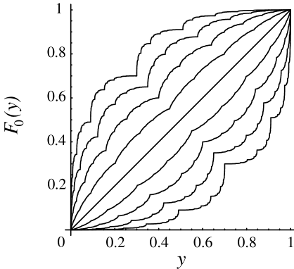
Figure 1. For the biased random walk of Example 1, $F_{0}$ is a Lebesgue singular function, obtained as the solution of Eq. (43), and which we display for values of $q$ ranging from $0.3$ (bottom curve) to $0.7$ (top curve). The straight line corresponds to $q=1/2$. Each curve was computed at $2^{10}$ points connected together by lines.

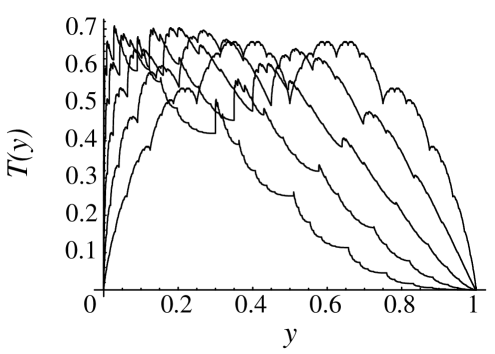
Figure 2. The generalized Takagi function for the biased random walk, Eq. (44). The parameter values range from $q=0.5$ which gives the original Takagi function, Eq. (42) (top curve at the right) to $q=0.7$ (bottom right). Each curve was computed at $2^{10}$ points connected together by lines.

5. Hausdorff Dimension of the Hydrodynamic modes

In this section, we investigate the fractal properties of the cumulative functions $F_{k}$ of the hydrodynamic modes for $k\neq 0$, as given by Eq. (28), and we compute their Hausdorff dimensions.

In order to compute the solutions of Eq. (28), we return to the symbolic dynamics and replace $y$ by the $r$-adic expansion, Eq. (10). We consider points $y$ with finite $r$-adic expansion $y=y(\omega_{1},\ldots,\omega_{l})$ and rewrite Eq. (28) in terms of the symbolic sequences :

$$F_{k}[y(\omega_{1},\ldots,\omega_{l})]=\sum_{j<\omega_{1}}\frac{p_{[j-(r-1)/2]}}{\chi_{k}}\;\exp\{-ik[j-(r-1)/2]\}\\ +\frac{p_{[\omega_{1}-(r-1)/2]}}{\chi_{k}}\;\exp\{-ik[\omega_{1}-(r-1)/2]\}\;F_{k}[y(\omega_{2},\ldots,\omega_{l})].$$ (45)

Starting with $F_{k}[\emptyset]=0$, we can successively compute

$$F_{k}[y(\omega_{1})],\quad F_{k}[y(\omega_{1},\omega_{2})],\quad F_{k}[y(\omega_{1},\omega_{2},\omega_{3})],\quad\text{etc}.$$

All these points are plotted in the complex plane where they form a fractal curve $({\rm Re}F_{k},{\rm Im}F_{k})$ similar to von Koch’s curve, under certain conditions (see the following examples).

Example 6.

Consider the triadic totally symmetric random walk of Example 2. From Eq. (34), the eigenvalues are found to be $\chi_{k}=(1/3)(1+2\cos k)$. The condition, Eq. (29), that Eq. (28) be contracting becomes $(1+2\cos k)>1$, which is satisfied as long as $-\pi/2<k<\pi/2$. In Fig. 3, we plot the imaginary versus real parts of $F_{k}$ for $k=0.1$ and $0.5$. The first of these two graphs for the smallest wavenumber $k=0.1$, Fig.3a, is dominated by the linear contributions to $F_{k}$, i.e. $F_{k}(y)\simeq y+ikT(y)$. As we argued in [27], the first order term in $k$, $T$, is the triadic equivalent of the Takagi function Eq. (42). In this case, $T(y)$ is solution of the functional equation

$$T(y)=\begin{cases}y+\frac{1}{3}T(3y),&0\leq y<\frac{1}{3},\\ \frac{1}{3}+\frac{1}{3}T(3y-1),&\frac{1}{3}\leq y<\frac{2}{3},\\ 1-y+\frac{1}{3}T(3y-2),&\frac{2}{3}\leq y<1.\end{cases}$$ (46)

The deviations – observed in Fig.3b – of the curve $({\rm Re}F_{k},{\rm Im}F_{k})$ with respect to the generalized Takagi function (46) are due to contributions which are second order in the wavenumber $k$. As we will show, these deviations are responsible for the fact that the Hausdorff dimension of this curve is not one for non-zero wavenumbers $k$. In fact, $D_{\rm H}(F_{k})>1$.

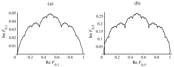
Figure 3. $F_{k}$ for the triadic totally symmetric random walk: (a) $k=0.1$; (b) $k=0.5$. The curves are computed at $3^{10}$ points connected together by lines.

Example 7.

Still considering the triadic totally symmetric random walk, we observe a rather spectacular fractal for the large wavenumber $k=\pi/3$ which corresponds to the eigenvalue $\chi_{\pi/3}=2/3$. This case is shown in Fig. 4. The points 0, 1/3, 2/3 and 1 are at the vertices of a half hexagon, which is responsible for the apparent hexagonal symmetry of this figure.

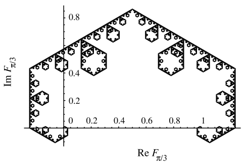
Figure 4. $F_{\pi/3}$ for the triadic totally symmetric random walk. The curve is computed at $3^{10}$ points, and connected together by lines.

Example 8.

Another interesting case corresponds to the critical value $k_{c}$ of $k$ for which Eq. (28) looses its contracting property, i.e. $\chi_{k_{c}}=p_{j}$ in one of the conditions (29). This leads to interesting solutions of Eq. (28). For instance, in the triadic totally symmetric random walk, $k_{c}=\pi/2$ yields

$$F_{\pi/2}(y)=\begin{cases}-iF_{\pi/2}(3y),&0\leq y<1/3,\\ -i+F_{\pi/2}(3y-1),&1/3\leq y<2/3,\\ 1-i+iF_{\pi/2}(3y-2),&2/3\leq y<1.\end{cases}$$ (47)

$F_{\pi/2}(y)$ is thus a non-continuous function of $y$. In the complex plane, the curve disintegrates into a disjoint set of points forming the square lattice ${\mathbb{Z}}^{2}$. Figure 5 displays this set constructed with the $3^{10}$ points $y(\omega_{1},\ldots,\omega_{10})$.

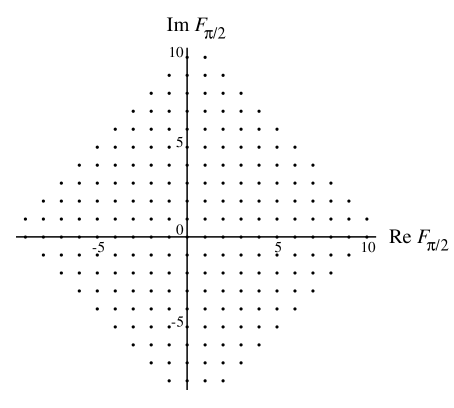
Figure 5. $F_{\pi/2}$ for the triadic totally symmetric random walk. The set is composed of the points of ${\mathbb{Z}}^{2}.$

Similar functions can be observed for the 2-adic and 5-adic totally symmetric random walks for $k_{c}=\pi/3$. In the 2-adic case, the set is a regular triangular lattice; in the 5-adic case, a regular hexagonal lattice.

We turn to the computation of the Hausdorff dimension of $F_{k}$, i.e., of the curve $({\rm Re}F_{k},{\rm Im}F_{k})$ drawn in the complex plane. The above examples show that the plot of $({\rm Re}F_{k},{\rm Im}F_{k})$ forms a continuous curve in the complex plane as long as $|k|<k_{c}$. However, the curve densely fills plain domains of the complex plane already for lower values of the wavenumber, $k_{f}<|k|<k_{c}$. For these values, the Hausdorff dimension of the curve saturates at the dimension two of the complex plane so that $D_{\rm H}(k)=2$ for $k_{f}\leq|k|<k_{c}$. At the limiting value $|k|=k_{f}$, the plot of $({\rm Re}F_{k},{\rm Im}F_{k})$ forms a fractal curve similar to the Lévy dragon which has a Hausdorff dimension equal to two [13, 33].

For still lower values of the wavenumber $|k|<k_{f}$, we consider the Hausdorff measure, $\Gamma_{l}^{d}(F_{k}),$ of the cylinder sets specified by the sequences $\{\omega_{1},\ldots,\omega_{l}\}$ :

$$\Gamma_{l}^{d}(F_{k})=\sum_{\omega_{1},\ldots,\omega_{l}}\Big{|}\Delta F_{k}[y(\omega_{1},\ldots,\omega_{l})]\Big{|}^{d},$$ (48)

where

$$\Delta F_{k}[y(\omega_{1},\ldots,\omega_{l})]=F_{k}[y(\omega_{1},\ldots,\omega_{l}+1)]-F_{k}[y(\omega_{1},\ldots,\omega_{l})],$$

with the notation

$$\{\omega_{1},\ldots,\omega_{l}+1\}=\begin{cases}\{\omega_{1},\ldots,\omega_{l-1},\omega_{l}+1\},&\omega_{l}<r-1,\\ \{\omega_{1},\ldots,\omega_{l-1}+1,0\},&\omega_{l}=r-1,\end{cases}$$ (49)

and we make the further convention that $y(r-1,\ldots,r-1,r)=1$. The quantities $\Delta F_{k}[y(\omega_{1},\ldots,\omega_{l})]$ are the segments of the curve, $({\rm Re}F_{k},{\rm Im}F_{k})$ at the $l^{\rm th}$ step of its construction. In the complex plane, the $l^{\rm th}$ approximant of the curve is covered by disks of diameter given by the absolute value of the segments $\Delta F_{k}[y(\omega_{1},\ldots,\omega_{l})]$, appearing on the right hand side of Eq. (48). We recall that the Hausdorff dimension, $D_{\rm H}(k),$ of $F_{k}$ is the value of $d$ such that [12]

$$\lim_{l\rightarrow\infty}\Gamma_{l}^{d}(F_{k})=\begin{cases}\infty,&d<D_{\rm H}(k),\\ 0,&d>D_{\rm H}(k).\end{cases}$$ (50)

With the help of Eq. (45), it is straightforward to check that

$$\Big{|}\Delta F_{k}[y(\omega_{1},\ldots,\omega_{l})]\Big{|} = \frac{\displaystyle{p_{[\omega_{1}-(r-1)/2]}}}{\displaystyle{|\chi_{k}|}}\Big{|}\Delta F_{k}[y(\omega_{2},\ldots,\omega_{l})]\Big{|},$$ (51)

$$= \frac{\displaystyle{1}}{\displaystyle{{|\chi_{k}|}^{l}}}\prod_{i=1}^{l}p_{[\omega_{i}-(r-1)/2]}.$$

Hence, the Hausdorff measure

$$\Gamma_{l}^{d}(F_{k})=\frac{\displaystyle{1}}{\displaystyle{{|\chi_{k}|}^{ld}}}\sum_{\omega_{1},\ldots,\omega_{l}}\prod_{i=1}^{l}{p_{[\omega_{i}-(r-1)/2]}}^{d}=\left(\frac{\displaystyle{1}}{\displaystyle{{|\chi_{k}|}^{d}}}\sum_{j=-(r-1)/2}^{(r-1)/2}{p_{j}}^{d}\right)^{l}.$$ (52)

According to Eq. (50), the Hausdorff dimension thus satisfies

$$|\chi_{k}|^{D_{\rm H}(k)}=p_{-(r-1)/2}^{D_{\rm H}(k)}+\dots+p_{(r-1)/2}^{D_{\rm H}(k)}.$$ (53)

Example 9.

For the triadic totally symmetric random walk, the Hausdorff dimension of $F_{\pi/3},$ shown in Fig. 4, satisfies

$$\bigg{(}\frac{\displaystyle{2}}{\displaystyle{3}}\bigg{)}^{D_{\rm H}(\pi/3)}=3\bigg{(}\frac{\displaystyle{1}}{\displaystyle{3}}\bigg{)}^{D_{\rm H}(\pi/3)}.$$

Therefore $D_{\rm H}(\pi/3)=\ln(3)/\ln(2)$.

Remark 3.

It is not possible to solve Eq. (53) and find a general expression for $D_{\rm H}(k)$ for all processes. However for the case of totally symmetric $r$-adic random walks for which $p_{j}=1/r,\;\forall j$, we can solve Eq. (53) and find

$$D_{\rm H}(k)=\begin{cases}\frac{\displaystyle{\ln(r)}}{\displaystyle{\ln(r\chi_{k})}}\;,&|k|<k_{f}\;,\\ 2\;,&k_{f}\leq|k|<k_{c}\;.\end{cases}$$ (54)

$k_{f}$ is the wavenumber such that $\chi_{k}=1/\sqrt{r}$ where the curve starts to densely fill the complex plane. $k_{c}$ is the wavenumber such that $\chi_{k}=1/r$, above which the cumulative function $F_{k}$ no longer forms a continuous curve in the complex plane. For the symmetric dyadic case $r=2$, the Hausdorff dimension (54) has been previously derived [39].

Example 10.

A numerical computation of Eq. (54) for the totally symmetric triadic random walk is shown in Fig. 6. In this case, $D_{\rm H}(k)=\ln(3)/\ln(1+2\cos k)$ for $|k|<k_{f}=1.1960...$, while $D_{\rm H}(k)=2$ for $k_{f}\leq|k|<k_{c}=\pi/2$.

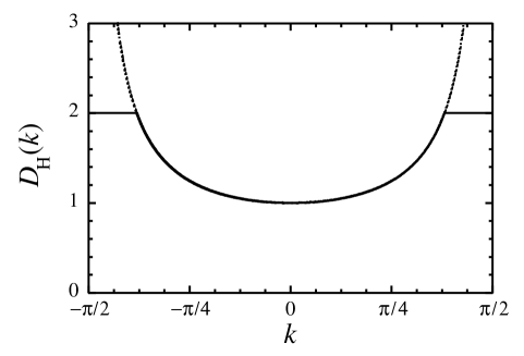
Figure 6. The Hausdorff dimension $D_{\rm H}$ for the triadic totally symmetric random walk, given by Eq. (54) with $r=3$. The dashed line depicts the extrapolation of $D_{\rm H}(k)$ outside of the interval $|k|<k_{f}=1.1960...$.

For small wavenumbers, i.e. $|k|\ll k_{f}$, we can expand the absolute value of the eigenvalue $\chi_{k}$, given by Eq. (26), in terms of the diffusion coefficient (33) of the general $r$-adic random walk :

$$|\chi_{k}|=1-{\mathcal{D}}k^{2}+O(k^{4}).$$ (55)

Notice that the absolute value of the eigenvalue does not depend on the drift velocity $v$ in the linear and quadratic terms of its expansion in powers of the wavenumber $k$.

To establish a connection between the diffusion coefficient and the Hausdorff dimension of the hydrodynamic modes (for which $|k|\ll k_{f}$), we let

$$D_{\rm H}(k)=1+ak^{2}+O(k^{4}),$$ (56)

and expand

$$\sum_{j}p_{j}^{D_{\rm H}(k)}=1+a\;k^{2}\;\sum_{j}p_{j}\;\ln p_{j}+O(k^{4}).$$ (57)

Substituting Eqs. (55) and (57) into Eq. (53), we find

$$a=\frac{\displaystyle{{\mathcal{D}}}}{\displaystyle{\sum_{j}p_{j}\;\ln p_{j}^{-1}}}=\frac{\displaystyle{{\mathcal{D}}}}{\displaystyle{\lambda^{+}}},$$ (58)

where $\lambda^{+}$ is the positive Lyapunov exponent (14) of our system.

We can thus state the following:

Theorem 1.

For an $r$-adic multi-baker map with probabilities $\{p_{-(r-1)/2},\linebreak\ldots,p_{(r-1)/2}\}$, the cumulative function of the hydrodynamic mode of wavenumber $k$, Eq. (28), forms in the complex plane a curve with the Hausdorff dimension

$$D_{\rm H}(k)=1+\frac{\displaystyle{{\mathcal{D}}}}{\displaystyle{\lambda^{+}}}\;k^{2}+O\big{(}k^{4}\big{)},$$ (59)

where $\lambda^{+}$ is the positive Lyapunov exponent (14) of this system and ${\mathcal{D}}$ is its diffusion coefficient as specified by Eq. (33).

As a corollary, we have the following:

Theorem 2.

Under the same conditions as in Theorem 1, the diffusion coefficient of the system is given in terms of the positive Lyapunov exponent $\lambda^{+}$ and the Hausdorff dimension $D_{\rm H}(k)$ of the cumulative function of the hydrodynamic mode of wavenumber $k$ according to

$${\mathcal{D}}=\lambda^{+}\lim_{k\to 0}\frac{D_{\rm H}(k)-1}{k^{2}}.$$ (60)

Remark 4.

The expression (60) bears a relation to the formula (2) giving the diffusion coefficient in terms of the Lyapunov exponent and the Hausdorff codimension of the fractal repeller ${\mathcal{R}}_{L}$ of orbits trapped in a 2-dimensional ordered Lorentz gas of size $L$ [19]. The analogy is best seen by writing Eq. (60) for a hydrodynamic mode of the smallest possible nonvanishing wavenumber $k=2\pi/L$ in a periodic chain of length $L$, whereupon Eq.(60) takes the form

$${\mathcal{D}}=\lim_{L\rightarrow\infty}\Big{(}\frac{\displaystyle{L}}{\displaystyle{2\pi}}\Big{)}^{2}\lambda^{+}\left[D_{\rm H}(2\pi/L)-1\right],$$ (61)

where $D_{\rm H}(2\pi/L)$ is the dimension of the fractal curve $F_{k}$ with $k=2\pi/L$. Although $ak^{2}$ in Eq. (56) plays a role very similar to the codimension $c_{\rm H}({\mathcal{R}}_{L})$ of Eq. (2), it cannot be identified as such because it is the coefficient of a correction to $D_{\rm H}$ above 1, which stems from the definition of $F_{k}$ as a cumulative function.

6. Conclusions

In this paper, we have shown with the help of simple models of deterministic diffusion that, in the last stages of the relaxation toward the stationary state, the hydrodynamic modes have cumulative functions with fractal Hausdorff dimensions. For small enough wavenumbers, we were able to derive an expression for the Hausdorff dimensions in terms of the diffusion coefficient and positive Lyapunov exponent of the system. Accordingly, the diffusion coefficient can be computed in terms of the Hausdorff dimension and the positive Lyapunov exponent, which is the content of Theorem 2.

Our formula (60) establishes a new relationship between the diffusion coefficient and the characteristic quantities of chaos, which generalizes both the equation (1) from the thermostated-system approach and the equation (2) from the escape-rate formalism, as anticipated in the Introduction. On the one hand, Eq. (60) remains applicable whether the system is thermostated (i.e., in the non-area-preserving case) or not (i.e., in the area-preserving case). On the other hand, no absorbing boundary is required in the present approach where Eq. (60) was derived. Accordingly, the number of particles is kept constant in systems to which Eq. (60) applies. In this regard, our new formula (60) unifies the previous formulae (1) and (2). The novelty of the present approach is to consider the Hausdorff dimension of an abstract curve in the complex plane, instead of the Hausdorff (or information) dimension of either an attractor or a repeller. This abstract curve is the cumulative function of the hydrodynamic mode of diffusion, which is a general concept of nonequilibrium statistical mechanics.

In view of the generality of the considerations developed in the present paper, we conjecture that Eq. (59) for the Hausdorff dimension of the hydrodynamic modes extends to spatially extended Axiom-A systems with two degrees of freedom which sustain transport by diffusion, and more generally to such chaotic systems with two degrees of freedom.

Moreover, the similarity between Eq. (2) and Eq. (61) of the escape-rate formalism suggests a generalization of our formalism to other transport processes. As shown by Dorfman and Gaspard [10, 20], the escape-rate formalism generalizes to other transport phenomena by setting up a first passage problem in the space of the Helfand moment [28]. In much the same way, we can infer that the eigendistributions of the time evolution in the space of the Helfand moment have cumulative functions with fractal Hausdorff dimensions given by a gradient expansion analogous to Eq. (59), where the diffusion coefficient is replaced by the corresponding transport coefficient. These questions will be addressed in more detail elsewhere.

References

- [1] Baranyai A., Evans D. J., and Cohen E. G. D., 1993. Field dependent conductivity and diffusion in a two-dimensional Lorentz gas. Journal of Statistical Physics 70, 1085.
- [2] Breymann W., Tél T., and Vollmer J., 1996. Entropy production for open dynamical systems. Physical Review Letters 77, 2945.
- [3] Breymann W., Tél T., and Vollmer J., 1998. Entropy balance, time reversibility, and mass transport in dynamical systems. Chaos 8, 396.
- [4] Chernov N. I., Eyink G. L., Lebowitz J. L., and Sinai Ya. G., 1993. Derivation of Ohm’s Law in a Deterministic Mechanical Model. Physical Review Letters 70, 2209.
- [5] Chernov N. I., Eyink G. L., Lebowitz J. L., and Sinai Ya. G., 1993. Steady state electric conductivity in the periodic Lorentz gas. Communications in Mathematical Physics 154, 569.
- [6] Chernov N. I. and Markarian R., 1997. Ergodic properties of Anosov maps with rectangular holes. Boletim da Sociedade Brasileira de Matemática 28, 271.
- [7] Chernov N. I. and Markarian R., 1997. Anosov maps with rectangular holes. Nonergodic cases. Boletim da Sociedade Brasileira de Matemática 28, 342.
- [8] Dellago Ch., Posch H. A., and Hoover W. G., 1996. Lyapunov instability in a system of hard disks in equilibrium and nonequilibrium steady states. Physical Review E 53, 1485.
- [9] Dettmann C. P., 2000. The Lorentz gas as a paradigm for nonequilibrium stationary states. In: D. Szasz, Editor. Hard Ball Systems and Lorentz Gas. Encycl. Math. Sci. (Berlin: Springer).
- [10] Dorfman J. R. and Gaspard P., 1995. Chaotic scattering theory of transport and reaction-rate coefficients. Physical Review E 51, 28.
- [11] Dorfman J. R., 1999. An Introduction to Chaos in Nonequilibrium Statistical Mechanics. (Cambridge UK: Cambridge University Press).
- [12] Eckmann J.-P. and Ruelle D., 1985. Ergodic theory of chaos and strange attractors. Review of Modern Physics 57, 617.
- [13] Edgar G. A., Editor, 1993. Classics on Fractals. (Reading MA: Addison-Wesley Publ. Co.).
- [14] Evans D. J. and Morriss G. P., 1990. Statistical Mechanics of Nonequilibrium Liquids. (London: Academic Press).
- [15] Evans D. J., Cohen E. G. D., and Morriss G. P., 1990. Viscosity of a simple fluid from its maximal Lyapunov exponents. Physical Review A 42, 5990.
- [16] Evans D. J., Cohen E. G. D., and Morriss G. P., 1993. Probability of second law violations in shearing steady states. Physical Review Letters 71, 2401.
- [17] Gaspard P. and Nicolis G., 1990. Transport Properties, Lyapunov Exponents, and Entropy per Unit Time. Physical Review Letters 65, 1693.
- [18] Gaspard P., 1992. Diffusion, effusion, and chaotic scattering: An exactly solvable Liouvillian dynamics. Journal of Statistical Physics 68, 673.
- [19] Gaspard P. and Baras F., 1995. Chaotic scattering and diffusion in the Lorentz gas. Physical Review E 51, 5332.
- [20] Gaspard P. and Dorfman J. R., 1995. Chaotic scattering theory, thermodynamic formalism and transport coefficients. Physical Review E 52, 3525.
- [21] Gaspard P., 1996. Hydrodynamic modes as singular eigenstates of the Liouvillian dynamics: Deterministic diffusion. Physical Review E 53, 4379.
- [22] Gaspard P., 1997. Entropy production in open, volume preserving systems. Journal of Statistical Physics 89, 1215.
- [23] Gaspard P., 1998. Chaos, Scattering, and Statistical Mechanics. (Cambridge UK: Cambridge University Press).
- [24] Gilbert T., 1999. Irreversible thermodynamics of reversible dynamical systems. (PhD thesis, University of Maryland, College Park, Maryland, USA).
- [25] Gilbert T. and Dorfman J. R., 1999. Entropy production , From open volume preserving to dissipative systems. Journal of Statistical Physics 96, 225.
- [26] Gilbert T., Ferguson C. D., and Dorfman J. R., 1999. Field driven thermostated system , a non-linear multi-baker map. Physical Review E 59, 364.
- [27] Gilbert T., Dorfman J. R., and Gaspard P., 2000. Entropy production, fractals, and relaxation to equilibrium. submitted to Physical Review Letters.
- [28] Helfand E., 1960. Transport Coefficients from Dissipation in a Canonical Ensemble. Physical Review 119, 1.
- [29] Hoover W. G., 1991. Computational Statistical Mechanics. (Amsterdam: Elsevier Science Publishers).
- [30] Kantz H. and Grassberger P., 1985. Repellers, semi-attractors, and long-lived chaotic transients. Physica D 17, 75.
- [31] von Koch H., 1904. Sur une courbe continue sans tangente obtenue par une construction géométrique élémentaire. Arkiv för Mathematik, Astronomi och Fysik 1, 681. Translated in [13].
- [32] von Koch H., 1906. Une méthode géométrique élémentaire pour l’étude de certaines questions de la théorie des courbes planes. Acta Mathematica 30, 145.
- [33] Lévy P., 1938. Les courbes planes ou gauches et les surfaces composées de parties semblables au tout. Journal de l’Ecole Polytechnique, série III, 7-8, pp. 227–247, pp. 249–291. Translated in [13].
- [34] Pianigiani G. and Yorke J., 1979. Expanding maps on sets which are almost invariant, decay and chaos. Trans. Amer. Math. Soc. 252, 351.
- [35] Posch H. A. and Hoover W. G., 1988. Lyapunov instability of dense Lennard-Jones fluids. Physical Review A 38, 473.
- [36] de Rham G., 1957. Sur un exemple de fonction continue sans dérivée. Enseignements Mathématiques 3, 71. Translated in [13].
- [37] Sinai Ya. G., 1979. Development of Krylov’s idea. Afterwards to, N. S. Krylov, 1979. Works on the foundations of statistical physics. (Princeton: Princeton University Press) pp. 239–281.
- [38] Takagi T., 1903. A simple example of the continuous function without derivative. Proceedings of the Physico-Mathematical Society of Japan 1, 176.
- [39] Tasaki S., Antoniou I., and Suchanecki Z., 1993. Deterministic diffusion, de Rham equation and fractal eigenvectors. Physics Letters A 179, 97.
- [40] Tasaki S. and Gaspard P., 1994. Fractal distribution and Fick’s law in a reversible chaotic system. In: M. Yamaguti, Editor. Towards the Harnessing of Chaos (Amsterdam: Elsevier) pp. 273–288.
- [41] Tasaki S. and Gaspard P., 1995. Fick’s law and fractality of nonequilibrium stationary states in a reversible multibaker map. Journal of Statistical Physics 81, 935.
- [42] Tasaki S., Gilbert T., and Dorfman J. R., 1998. An analytic construction of the SRB measures for baker-type maps. Chaos 8, 424.
- [43] Tasaki S. and Gaspard P., 1999. Thermodynamic behavior of an area-preserving multibaker map with energy. Theoretical Chemistry Accounts 102, 385.
- [44] Tél T., Vollmer J., and Breymann W., 1996. Europhysics Letters 35, 659.
- [45] Tél T. and Vollmer J., 2000. Entropy Balance, Multibaker Maps, and the Dynamics of the Lorentz Gas. In: D. Szasz, Editor. Hard Ball Systems and Lorentz Gas. Encycl. Math. Sci. (Berlin: Springer).
- [46] van Beijeren H. and Dorfman J. R., 1995. Lyapunov exponents and Kolmogorov-Sinai entropy for the Lorentz gas at low densities. Physical Review Letters 74, 4412.
- [47] van Beijeren H. and Dorfman J. R., 1996. Lyapunov exponents and Kolmogorov-Sinai entropy for the Lorentz gas at low densities, Erratum. Physical Review Letters 76, 3238.
- [48] van Beijeren H., Dorfman J. R., Posch H. A., and Dellago Ch., 1997. Kolmogorov-Sinai entropy for dilute gases in equilibrium. Physical Review E 56, 5272.
- [49] Vollmer J., Tél T., and Breymann W., 1997. Equivalence of irreversible entropy production in driven systems: An elementary chaotic map approach. Physical Review Letters 79, 2759.
- [50] Vollmer J., Tél T., and Breymann W., 1998. Entropy balance in the presence of drift and diffusive currents: An elementary map approach. Physical Review E 58, 1672.