Visualization of correlation cascade in spatio-temporal chaos using wavelets

Abstract

We propose a simple method to visualize spatio-temporal correlation between scales using wavelets, and apply it to two typical spatio-temporally chaotic systems, namely to coupled complex Ginzburg-Landau oscillators with diffusive interaction, and those with non-local interaction. Reflecting the difference between underlying dynamical processes, our method provides distinctive results for those two systems. Especially, for the non-locally interacting case where the system exhibits fractal amplitude patterns and power-law spectrum, it clearly visualizes the dynamical cascade process of spatio-temporal correlation between scales.

^∗ Corresponding author.
  E-mail: nakao@mns.brain.riken.go.jp

05.45.-a

I Introduction

It has long been a subject of discussion how to capture and describe complex dynamical processes of strongly correlated many-body systems that are ubiquitous in nature. Probably one of the most important problems of such kind at present is the one faced in neuroscience. In what way biological information processing is encoded into spikes of neurons in the brain is the greatest mystery of present neuroscience. In order to capture subtle correlation between activities of neurons, information-theoretical techniques have been developed and applied to experimental signals [Rieke et al., 1998].

On the other hand, we may mention Richardson’s cascade picture of fully-developed fluid turbulence as a successful example of capturing the essence of a strongly correlated system, which stated that large eddies gradually fragment into smaller eddies, and eventually dissipate due to viscosity. Apart from the difficult problem of intermittency, this picture was mathematically formulated into the Kolmogorov 1941 theory, which gave the famous $-5/3$ energy spectrum [Frisch, 1995]. This success was due to the fact that in fluid turbulence, fortunately, a simple hierarchy in spatial scale (or equivalently, in temporal / energy scales) is formed as a result of complex nonlinear dynamics of a number of modes. Since the success in fluid turbulence, attempts have been made to capture the dynamics of other kinds of many-body systems such as spatio-temporal chaos [Ikeda & Matsumoto, 1989], chaotic systems with large degrees of freedom [Kaneko, 1994], and stock markets [Arnéodo et al., 1998a], based on the picture that energy, or more generally information or causality, flows from scales to scales.

In analyzing space-scale properties of various kinds of signals, the wavelet transform is expected to be a useful tool due to its localized nature both in space and scale, and many applications have been made [Mallat, 1999]. Of course, there are many studies that tried to capture the cascade process of fully-developed turbulence directly using wavelets [Argoul et al., 1989; Yamada & Ohkitani, 1991; Arnéodo et al., 1998b]. But most of the studies treated one-dimensional time sequences of the velocity field measured at a single point in fluid, and rather a limited number of studies actually investigated the temporal evolution of correlation between scales of spatially extended fields [Toh, 1995].

In this paper, we propose a simple visualization method of such spatio-temporal correlation between scales of spatially extended fields using wavelets, and apply it to two typical spatio-temporally chaotic systems. As such chaotic systems, we investigate ordinary diffusively coupled complex Ginzburg-Landau oscillators [Kuramoto, 1984; Bohr et al., 1998] and somewhat unusual non-locally coupled complex Ginzburg-Landau oscillators [Kuramoto, 1995]. While the former system exhibits spatially smooth amplitude patterns, the latter system exhibits fractal spatial patterns. Therefore, the dynamical processes behind those systems are expected to differ from each other significantly, and it is interesting to see whether their difference can be detected by our method or not.

II Coupled complex Ginzburg-Landau oscillators

The ordinary diffusively (i.e., locally) coupled complex Ginzburg-Landau equation [Kuramoto, 1984; Bohr et al., 1998] is given by

$$\dot{W}(x,t)=W-(1+ic_{2})|W|^{2}W+D(1+ic_{1})\nabla^{2}W,$$ (1)

which can be derived, for example, from equations of oscillatory media in the vicinity of their Hopf bifurcation points by the center-manifold reduction technique. Here, $W(x,t)$ is a complex amplitude of an oscillator at position $x$ and at time $t$, $c_{1}$ and $c_{2}$ are real parameters, and $D$ is a diffusion constant. It is well known that this equation exhibits spatio-temporal chaos in some appropriate parameter region. We call this equation “LCGL equation” hereafter.

In this paper, we treat only spatially one-dimensional cases. We fix the length of the system at $L=1$, and assume a periodic boundary condition. The diffusion constant is set at $D=0.0035$, and the parameters are fixed at $c_{1}=-2$ and $c_{2}=2$. With these values, the spatially uniform solution of the LCGL equation is unstable, and the system exhibits spatio-temporal chaos. Typical time scale of the system is roughly estimated as the time needed for an uncoupled free oscillator to go around its limit cycle, and is given by $2\pi/c_{2}\simeq 3$. The numerical simulation was done in wavenumber space using $N=2^{10}-2^{14}$ modes by the pseudo-spectral method with a time step of $0.01$ (Euler integration).

Due to the existence of a diffusion term, the solution of the LCGL equation necessarily possesses a characteristic minimal length scale, below which fluctuations are strongly depressed. Thus, the amplitude pattern $|W(x,t)|$ of the solution has a smoothly modulated shape as displayed in Fig. 1. The shortest wavelength determined by the diffusion constant is about $\sqrt{D}\simeq 0.06\simeq 1/16$. For the sake of comparison, this value is equated with the coupling length of the non-locally coupled system that we explain later. Figure 2 displays temporal evolution of the amplitude pattern, and Fig. 3 shows its power spectrum. Since short-wavelength components are strongly depressed, the power spectrum decays exponentially.

FIG. 1.: Snapshot of the amplitude field $|W(x,t)|$ of the LCGL equation. $N=2^{10}$ modes are used in the numerical calculation.

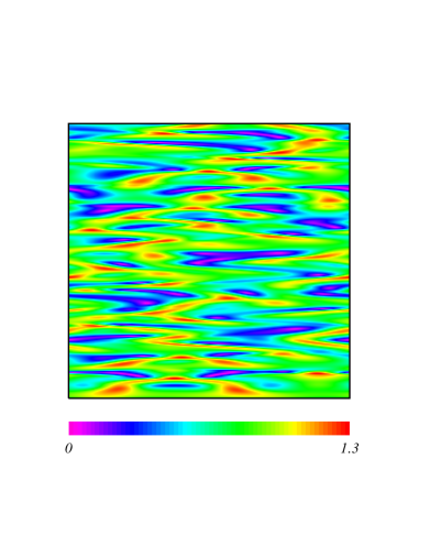
FIG. 2.: Evolution of the amplitude field of the LCGL equation. The horizontal axis indicates the spatial coordinate $x\;(0\leq x<1)$, and the vertical axis the time $t\;(0\leq t<125)$. Time increases upwards. Initial transient is discarded.

FIG. 3.: Power spectrum of the amplitude field of the LCGL equation. The inset shows semi-log plot of the same spectrum.

As another spatio-temporally chaotic system, we investigate a different type of coupled complex Ginzburg-Landau oscillators, which was first introduced by Kuramoto [1995]. Instead of a diffusive interaction, it has a non-local interaction; each oscillator feels a non-local mean field of other oscillators through a kernel $g(|x|)$, which is a decreasing function of $|x|$. Hereafter we use $g(|x|)=g_{0}\exp(-|x|/\gamma)$ as the kernel, where $\gamma$ gives the coupling range. $g_{0}$ is some appropriate normalization constant, and assumed to be $2\gamma$. The equation for this system of non-locally coupled oscillators is given by

$$\dot{W} (x,t)=W-(1+ic_{2})|W|^{2}W$$ (4)

$$+K(1+ic_{1})\int dx^{\prime}g(|x^{\prime}-x|)\left[W(x^{\prime},t)-W(x,t)\right],$$

which we call “NCGL equation” hereafter. This equation can be derived, for example, from a model of oscillatory biological cells that are interacting through some diffusive chemical substance with a finite decay rate.

Although the difference between this NCGL equation and the LCGL equation is only the last interaction term, it was shown that this NCGL equation exhibits spatio-temporal chaos with remarkably different features from the LCGL equation, such as fractal amplitude patterns, power-law spatial correlation, and power-law spectrum. We again fix the length of the system at $L=1$, and assume a periodic boundary condition. The coupling range is fixed at $\gamma=1/16$, which is equal to the shortest characteristic length $\sqrt{D}\simeq 1/16$ of the LCGL equation. (More precisely, by assuming the smoothness of the amplitude field $W(x^{\prime},t)$ in the interaction term and expanding it up to the second order in $x^{\prime}-x$ around $x$, we obtain an effective diffusion constant $D_{eff}=K\gamma^{2}$ for the NCGL equation. However, the smoothness of the amplitude field is not always guaranteed, hence this correspondence is only formal.) The parameter values are again set at $c_{1}=-2$ and $c_{2}=2$. With these values, the uniform solution of the system is always unstable, and the system behaves in a chaotic manner. Further, the behavior of the system strongly depends on the remaining coupling strength $K$; the amplitude pattern of the system is smooth for large $K$ ($\sim 1.5$), while almost discontinuous for small $K$ ($\sim 0.5$). Between these values, there exists a parameter region where the amplitude pattern is fractal, and its spatial correlation exhibits power-law behavior. We fix $K=0.9$ hereafter, where the system is exactly in this “anomalous” spatio-temporally chaotic regime. The numerical simulation was done in real space using $N=2^{10}-2^{14}$ oscillators by the 4th-order Runge-Kutta method with a time step of $0.05$.

Figure 4 displays a typical snapshot of the solution of the NCGL equation, and Fig. 5 shows its temporal evolution. In contrast to the case of the LCGL equation, the amplitude pattern is not completely smooth, but is composed of patches of smooth coherent regions and strongly disordered regions. The power spectrum displayed in Fig. 6 also indicates the difference clearly. It exhibits power-law decay rather than the exponential decay in the case of the LCGL equation, which implies the strong anomaly of the amplitude field. Actually, it was shown that the amplitude pattern of the NCGL equation is fractal, and its fractal dimension varies with the coupling strength $K$. These properties are essentially the results of the absence of length scale shorter than the coupling range $\gamma$, and can be explained using a simple multiplicative stochastic model to a certain extent [Kuramoto & Nakao, 1996].

FIG. 4.: Snapshot of the amplitude field $|W(x,t)|$ of the NCGL equation. $N=2^{10}$ oscillators are used in the numerical calculation.

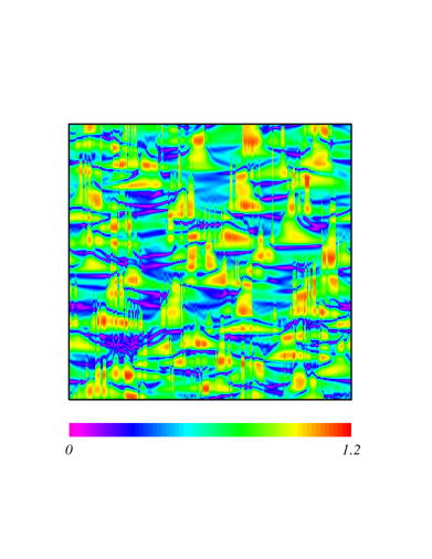
FIG. 5.: Evolution of the amplitude field of the NCGL equation. The horizontal axis indicates the spatial coordinate $x\;(0\leq x<1)$, and the vertical axis the time $t\;(0\leq t<125)$. Time increases upwards. Initial transient is discarded.

FIG. 6.: Power spectrum of the amplitude field of the NCGL equation. The inset shows log-log plot of the same spectrum.

Thus, the difference in the interaction term greatly changes the amplitude pattern of the system, even though the oscillators and characteristic length scales are the same. Especially, the power-law behavior of the power spectrum reminds us of the $-5/3$ energy spectrum of fluid turbulence. (However, the exponent changes with the coupling strength $K$ for our NCGL equation.) The power-law behavior of the energy spectrum in fluid turbulence is related to the cascade process of breakdown of vortices. Thus, we may naively expect that our NCGL equation also possesses some kind of cascade process. Of course, the NCGL equation is strongly dissipative and there is no such conservative quantity like energy or enstrophy. However, we still expect a cascade process of some quantity from long-wavelength components to shorter-wavelength components, which may be called causality or information, or merely correlation. In the following part of this paper, we develop a simple method to visualize the spatio-temporal correlation between fluctuations at different scales, in order to prove the existence of such cascade process.

III Wavelet-based correlation analysis

Let us consider decomposing the spatial pattern into various scales using wavelets, and analyzing the temporal correlation between them. We decompose a spatial pattern $V(x)$ using an orthonormal wavelet basis as

$$V(x)=\sum_{j=-\infty}^{\infty}\sum_{k=-\infty}^{\infty}a_{j,k}\psi_{j,k}(x),$$ (5)

where $a_{j,k}$ is an expansion coefficient, and $\psi_{j,k}(x)$ is a child wavelet generated from the mother wavelet $\psi(x)$ by translation and dilation as

$$\psi_{j,k}(x)=\sqrt{2^{j}}\psi(2^{j}x-k),$$ (6)

where $j$ is a scale parameter, and $k$ is a translation parameter. The child wavelets are mutually orthogonal as

$$\langle\psi_{j,k},\psi_{j^{\prime},k^{\prime}}\rangle=\int_{-\infty}^{\infty}\psi_{j,k}(x^{\prime})\psi^{*}_{j^{\prime},k^{\prime}}(x^{\prime})dx^{\prime}=\delta_{j,j^{\prime}}\delta_{k,k^{\prime}},$$ (7)

and form a complete orthonormal set. Since the child wavelet $\psi_{j,k}(x)$ is localized both in space and scale roughly at position $k/2^{j}$ and scale $1/2^{j}$, the expansion coefficient given by

$$a_{j,k}=\langle V,\psi_{j,k}\rangle=\int_{-\infty}^{\infty}V(x^{\prime})\psi^{*}_{j,k}(x^{\prime})dx^{\prime}$$ (8)

quantifies the magnitude of fluctuation of $V(x)$ around this space-scale point. Hereafter we use Meyer’s wavelet. It is a real analytic function that decays faster than any power function as $|x|\to\infty$, and its moment of any order vanishes, i.e.,

$$\int_{-\infty}^{\infty}x^{n}\psi(x)dx=0,\;\;\;(n\geq 0).$$ (9)

Further, it has a smooth Fourier transform with a compact support. These features are very preferable from the viewpoint of physicists. For the details of Meyer’s wavelet and efficient numerical algorism, see Refs. [Yamada & Ohkitani, 1991; Mallat, 1999]. Meyer’s mother wavelet and one of its child wavelet are shown in Fig. 7.

FIG. 7.: Meyer’s wavelets; mother wavelet ($j=0$, $k=0$) and one of its child wavelet ($j=1$, $k=4$).

In the practical numerical calculation, the amplitude pattern is a periodic function on $[0,1)$ represented by $N=2^{n}$ discrete points. Therefore, we extend the pattern over the whole real axis by a periodic extrapolation in order to apply the wavelet transform. Consequently, in the actual numerical calculation, the first subscript $j$ in the summation of Eq. (5) indicating the scale runs from $0$ to $n-1$, and the second subscript $k$ indicating the translation runs from $0$ to $2^{j}-1$.

Rather than using the obtained expansion coefficient directly, we define a new coarse-grained field $b_{j}(x)\;(0\leq x<1)$ by a piecewise constant interpolation from the expansion coefficient $a_{j,k}$ as

$$b_{j}(x)=\log|a_{j,k}|^{2}\;\;\left(\frac{k}{2^{j}}\leq x<\frac{k+1}{2^{j}},\;\;k=0,1,...,2^{j}-1\right).$$ (10)

Here we take a square of the coefficient, because we are interested in the absolute intensity of the fluctuation at a certain position and scale. Further taking the logarithm is merely for convenience sake here; we obtain similar results without taking the logarithm. However, there also exists some discussion claiming that taking the logarithm is more appropriate when the system under consideration possesses a random multiplicative process [Arnéodo et al., 1998a; Arnéodo et al., 1998b], and the NCGL equation is actually considered this case. Figures 8 and 9 display the coarse-grained fields $b_{j}(x)$ for the LCGL and NCGL equations. The obtained data for the LCGL equation are very noisy for large $j$ values, since components whose wavelengths are shorter than the dissipation scale $\sqrt{D}\simeq 1/16$ decay very quickly. On the other hand, we can observe clear positional correlation between scales down to a very small wavelength in the case of the NCGL equation.

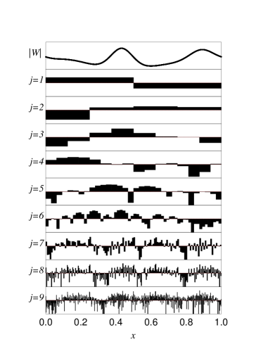
FIG. 8.: Coarse-grained field $b_{j}(x)$ obtained from the logarithm of the squared wavelet coefficient of the LCGL equation. The top panel shows the original amplitude pattern $|W(x)|$. The scale $j$ ranges from $1$ to $9$ from above. Each graph is normalized with its mean and variance. $N=2^{10}$ modes are used in the numerical calculation.

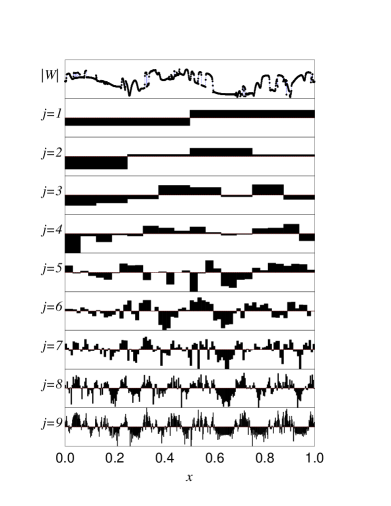
FIG. 9.: Coarse-grained field $b_{j}(x)$ obtained from the logarithm of the squared wavelet coefficient of the NCGL equation. The top panel shows the original amplitude pattern $|W(x)|$. The scale $j$ ranges from $1$ to $9$ from above. Each graph is normalized with its mean and variance. $N=2^{10}$ oscillators are used in the numerical calculation.

Let $V_{1}(x)$ be the amplitude pattern at time $t$, i.e., $V_{1}(x)=|W(x,t)|$, and $V_{2}(x)$ be the amplitude pattern evolved from $V_{1}(x)$ for a period of $\Delta t$, i.e., $V_{2}(x)=|W(x,t+\Delta t)|$. From these amplitude patterns, we obtain coarse-grained fields $b^{1}_{j_{1}}(x)$ and $b^{2}_{j_{2}}(x)$ at scales $j_{1}$ and $j_{2}$. We then define deviations of these fields from their mean values as

$$\Delta b^{1}_{j_{1}}(x)=b^{1}_{j_{1}}(x)-\overline{(b^{1}_{j_{1}},I)},$$ (11)

and

$$\Delta b^{2}_{j_{2}}(x)=b^{2}_{j_{2}}(x)-\overline{(b^{2}_{j_{2}},I)},$$ (12)

where $I$ is a constant-valued function $I(x)\equiv 1$, and the inner product of $f(x)$ and $g(x)$ is defined as

$$(f,g)=\int_{0}^{1}f(x)g(x)dx.$$ (13)

Now we define a kind of cross-correlation matrix $C_{j_{1},j_{2}}(\Delta t)$ from these $\Delta b^{1}_{j_{1}}(x)$ and $\Delta b^{2}_{j_{2}}(x)$ as

$$C_{j_{1},j_{2}}(\Delta t)=\frac{\overline{(\Delta b^{1}_{j_{1}},\;\Delta b^{2}_{j_{2}})}}{\left[\;\overline{(\Delta b^{1}_{j_{1}},\;\Delta b^{1}_{j_{1}})}\;\overline{(\Delta b^{2}_{j_{2}},\;\Delta b^{2}_{j_{2}})}\;\right]^{1/2}}.$$ (14)

From this definition, $C_{j_{1},j_{2}}(\Delta t)=C_{j_{2},j_{1}}(-\Delta t)$ obviously follows. The overlines in the above equations indicate temporal average, assuming the stationarity of the spatio-temporal chaos under consideration.

When $\Delta t=0$, $V_{2}(x)$ represents the same amplitude pattern as $V_{1}(x)$. Thus $\Delta b^{1}_{j_{1}}(x)$ and $\Delta b^{2}_{j_{2}}(x)$ are identical, and $C_{j_{1},j_{2}}$ is merely a symmetric matrix. When $\Delta t\neq 0$, $V_{2}(x)$ differs from $V_{1}(x)$ to some degree depending on $\Delta t$. Therefore $C_{j_{1},j_{2}}$ is no longer symmetric, and its asymmetry is expected to characterize the variation of spatio-temporal correlation between scales. In order to see this asymmetry clearly, let us decompose the matrix $C_{j_{1},j_{2}}$ into symmetric and antisymmetric parts as

$$D_{j_{1},j_{2}}(\Delta t)=\frac{1}{2}\left\{C_{j_{1},j_{2}}(\Delta t)+C_{j_{2},j_{1}}(\Delta t)\right\},$$ (15)

and

$$E_{j_{1},j_{2}}(\Delta t)=C_{j_{1},j_{2}}(\Delta t)-C_{j_{2},j_{1}}(\Delta t).$$ (16)

The symmetric part $D_{j_{1},j_{2}}$ is invariant under time-reversal transform $\Delta t\leftrightarrow-\Delta t$, while the antisymmetric part $E_{j_{1},j_{2}}$ is not invariant (antisymmetric). Thus the matrix $E_{j_{1},j_{2}}$ is expected to quantify the variation of spatio-temporal correlation between scales that is not symmetric to time-reversal, namely, to give a certain measure of the flow of information or correlation between scales.

In Fig. 10, the symmetric part $D_{j_{1},j_{2}}$ and the antisymmetric part $E_{j_{1},j_{2}}$ of the correlation matrix obtained for the LCGL equation are displayed using color codes for several values of the time difference $\Delta t$. The top row displays results obtained for the same time ($\Delta t=0$), and the lower rows display results for larger values of the time difference $\Delta t$. The vertical axis of each graph represents the scale $j_{1}$ of the pattern at the reference time, and the horizontal axis represents the scale $j_{2}$ of the pattern $\Delta t$ after the reference time. First, for $\Delta t=0$, the antisymmetric part is merely zero and only the symmetric part takes positive values. The diagonal components naturally take largest values, since the self-correlation of the fluctuation at the same scale is strongest. Besides, it can be seen that there exists rather strong correlation between adjacent scales in the dissipation region determined by the diffusion constant $D$ (the region with the scale slightly smaller than $j\simeq 4$). When the time difference $\Delta t$ becomes a little larger, the symmetric part diminishes. But still the diagonal components and the dissipation region maintain higher correlations than the others. Now, if we look at the antisymmetric part, there appear small localized regions in the neighborhood of the dissipation region across the diagonal, which have negative and positive correlations, respectively. This implies that fluctuation at a certain scale at the reference time (vertical axis) possesses relatively strong correlation to fluctuation at slightly smaller scale $\Delta t$ after the reference time (horizontal axis). In this case, it can be considered as visualizing the dissipation due to the diffusion term. As the time difference $\Delta t$ becomes further large, both the symmetric and antisymmetric parts tend to take smaller values, and correlation between the patterns vanishes. The intensity of the antisymmetric part is typically $20\%$ of the symmetric part at its maximum.

Figure 11 displays the symmetric part $D_{j_{1},j_{2}}$ and the antisymmetric part $E_{j_{1},j_{2}}$ of the correlation matrix obtained for the NCGL equation for several values of the time difference $\Delta t$ using color codes, as in the case of Fig. 10. When there is no time difference ($\Delta t=0$), only the symmetric part takes finite values, and its diagonal components take largest values as in the case of the LCGL equation. However, the region where the correlation between adjacent scales takes its peak value is located at much smaller scale. When the time difference $\Delta t$ becomes a little larger, the difference becomes more remarkable; there appear wide coherent regions with positive and negative correlation, which spread over scales shorter than the characteristic length of the system ($j\simeq 4$) determined by the coupling range $\gamma$. This asymmetry is maintained up to a considerably large value of $\Delta t$, which indicates that long-wavelength components at the reference time maintain strong correlations widely to shorter-wavelength components at later times. As we increase the time difference $\Delta t$ further, the correlation between scales gradually vanishes from the long-wavelength region. But it takes much longer than the case of the LCGL equation. These facts suggest the existence of cascade-like propagation of some quantity from long wavelength to shorter wavelength. The maximum intensity of the antisymmetric part is about $10\%$ of the symmetric part.

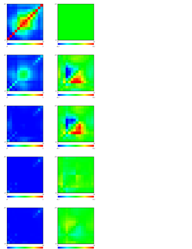
FIG. 10.: Evolution of the symmetric part $D_{j_{1},j_{2}}$ (left column) and the antisymmetric part $E_{j_{1},j_{2}}$ (right column) of the correlation matrix with the time difference $\Delta t$ for the LCGL equation. In each figure, the vertical axis indicates the scale $j_{1}$ at the reference time, and the horizontal axis indicates the scale $j_{2}$ at the time $\Delta t$ after the reference time. The scales of both axes range from $0$ to $13$. Time intervals between patterns are $\Delta t=0,1,2,4,8$ from the top. $N=2^{14}$ modes are used in the numerical calculation. The color scale of $D_{j_{1},j_{2}}$ is from $0$ (blue) to $1$ (red), while that of $E_{j_{1},j_{2}}$ is from $-0.1$ (blue) to $0.1$ (red).

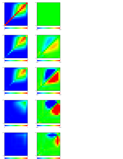
FIG. 11.: Evolution of the symmetric part $D_{j_{1},j_{2}}$ (left column) and the antisymmetric part $E_{j_{1},j_{2}}$ (right column) of the correlation matrix with the time difference $\Delta t$ for the NCGL equation. In each figure, the vertical axis indicates the scale $j_{1}$ at the reference time, and the horizontal axis indicates the scale $j_{2}$ at the time $\Delta t$ after the reference time. The scales of both axes range from $0$ to $13$. Time intervals between patterns are $\Delta t=0,2,5,20,40$ from the top. $N=2^{14}$ oscillators are used in the numerical calculation. The color scale of $D_{j_{1},j_{2}}$ is from $0$ (blue) to $1$ (red), while that of $E_{j_{1},j_{2}}$ is from $-0.05$ (blue) to $0.05$ (red).

In order to see the temporal evolution of the antisymmetric part of the correlation matrix in more detail, antisymmetric components $E_{j,j+1}$ between adjacent scales $j$ and $j+1$ normalized by the maximum value at each scale are displayed in Figs. 12 and 13 for scales smaller than the characteristic length. In the case of the LCGL equation, there is no clear ordering of the temporal variation of correlation. Each curve has its maximum at some small value of $\Delta t$, and vanishes quickly. In the case of the NCGL equation, on the other hand, there exists a clear time ordering of the curves in scale; the correlation between long-wavelength fluctuation (small $j$ values) becomes large earlier and decreases quickly, while the correlation between short-wavelength fluctuation (large $j$ values) becomes large later and decreases very slowly. (Note the difference of time scale between the graphs for the LCGL and NCGL equations.)

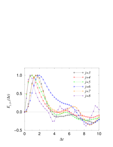
FIG. 12.: Antisymmetric part of the correlation coefficient $E_{j,j+1}$ between two successive scales $j$ and $j+1$ as a function of the time interval $\Delta t$ for the LCGL equation. Each curve is normalized by its maximum value.

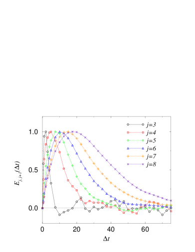
FIG. 13.: Antisymmetric part of the correlation coefficient $E_{j,j+1}$ between two successive scales $j$ and $j+1$ as a function of the time interval $\Delta t$ for the NCGL equation. Each curve is normalized by its maximum value.

IV Discussion

As we demonstrated, our simple method based on the correlation matrix seems to visualize the spatio-temporal correlation between scales of spatio-temporal chaos successfully. Our method clearly visualized the difference of dynamical process between two systems with different natures. Especially, for the non-locally coupled system, it verified the existence of cascade-like propagation of correlation from long-wavelength components to shorter-wavelength components.

First, the use of the wavelet transform is essential for our results. It seems difficult to obtain similar results using a method that flattens out the spatial information completely, like the Fourier transform. As can clearly be seen from the definition of the inner product given in Eq. (13), our method captures the simultaneous fluctuation of two fields at the same position in space. For example, if we use a different definition of the inner product that loses the spatial information by taking spatial average of each field first, we cannot observe the correlation between scales so clearly as in Figs. 10 and 11. Similarly, if we change the definition of the inner product so as to multiply the fields with their origins shifted by half the system size, the correlation matrix almost vanishes. (This tendency is more remarkable for the NCGL equation. In the case of the LCGL equation, though not so clear, we obtain similar asymmetric correlation matrices with these modified definitions of the inner product. This is because with the values of $D$ and $L$ we used in our calculation, the ratio of the diffusion constant to the system size is considerably large, and some coherence over the whole system still remains. If we further decrease the value of $D$, the correlation matrix tends to vanish as in the case of the NCGL equation.)

Conversely, the fact that we succeeded in visualization using the definition of the inner product given in Eq. (13) implies that the cascade process occurs in spatially localized regions in our system. However, it is frequently seen in other systems that the spatial structure of the pattern collapses while moving constantly, as in the case of convective instability. In order to detect such phenomena, it would be possible to generalize the definition of the inner product in such a way that the distance between the origins of the fields is increased with $\Delta t$.

Precisely speaking, the result visualized by our method is not a flow of causality, but merely a flow of correlation. Namely, it indicates that fluctuation at the reference time at some scale varies in unison with fluctuation at the later time at some other scale, but it does not necessarily mean that the former one actually affects the latter one. Of course, it is natural to interpret it as causality in our cases. But in order to be exact, it will be possible to perturb a certain mode at some scale, e.g. by using a sinusoidal wave, and visualize the propagation of its aftereffect to prove that it is indeed a causal relationship.

Finally, though we did not give a detailed discussion in this paper, we will be able to investigate the dynamical process of the spatio-temporal chaos of non-locally coupled oscillators in more detail by quantitatively analyzing the results obtained by our method. For example, from the peak positions of the $E_{j,j+1}$ curves shown in Fig.13, we will be able to study the dependence of characteristic time scale of the underlying cascade process on the coupling strength. Such a study will also be an interesting future subject.

REFERENCES

- [1] Argoul, F., Arnéodo, A., Grasseau, G., Gagne, Y., Hopfinger, E. J. & Frisch, U. [1989] “Wavelet analysis of turbulence reveals the multifractal nature of the Richardson cascade”, Nature 338, 51-53.
- [2] Arnéodo, A., Muzy, J.-F. & Sornette, D. [1998a] “”Direct” causal cascade in the stock market”, Eur. Phys. J. B 2, 277-282.
- [3] Arnéodo, A., Bacry, E., Manneville, S. & Muzy, J. F. [1998b] “Analysis of random cascades using space-scale correlation functions”, Phys. Rev. Lett. 80, 708-711.
- [4] Bohr, T., Jensen, M. H., Paladin, G. & Vulpiani, A. [1998] Dynamical Systems Approach to Turbulence (Cambridge University Press, Cambridge).
- [5] Frisch, U. [1995] Turbulence, the legacy of A. N. Kolmogorov (Cambridge University Press, Cambridge).
- [6] Ikeda, K. & Matsumoto, K. [1989] “Information theoretical characterization of turbulence”, Phys. Rev. Lett. 62, 2265-2268.
- [7] Kaneko, K. [1994] “Information cascade with marginal stability in a network of chaotic elements”, Physica D 77, 456-472.
- [8] Kuramoto, Y. [1984] Chemical Oscillations, Waves, and Turbulence (Springer-Verlag, Berlin); Mori, H. & Kuramoto, Y. [1998] Dissipative Structures and Chaos (Springer-Verlag, Berlin).
- [9] Kuramoto, Y. [1995] “Scaling behavior of turbulent oscillators with non-local interaction”, Prog. Theor. Phys. 94, 321-330.
- [10] Kuramoto, Y. & Nakao, H. [1996] “Origin of power-law spatial correlations in distributed oscillators and maps with nonlocal coupling”, Phys. Rev. Lett. 76, 4352-4355.
- [11] Mallat, S. [1999] A Wavelet Tour of Signal Processing (Academic Press, San Diego).
- [12] Rieke, F., Warland, D., van Steveninck, R. R. & Bialek, W. [1998] Spikes (MIT Press, Cambridge).
- [13] Toh, S. [1995] “Time correlation between entropy and/or energy distributed into scales by 2D wavelet in 2D free-convective turbulence”, J. Phys. Soc. Japan 64, 685-689.
- [14] Yamada, M. & Ohkitani, K. [1991] “An identification of energy cascade in turbulence by orthonormal wavelet analysis”, Prog. Theor. Phys. 86, 799-815; [1991] “Orthonormal wavelet analysis of turbulence”, Fluid Dynamics Research 8, 101-115.