“EFFECTIVE” FITNESS LANDSCAPES FOR EVOLUTIONARY SYSTEMS

Abstract

In evolution theory the concept of a fitness landscape has played an important role, evolution itself being portrayed as a hill-climbing process on a rugged landscape. In this article it is shown that in general, in the presence of other genetic operators such as mutation and recombination, hill-climbing is the exception rather than the rule. This descrepency can be traced to the different ways that the concept of fitness appears — as a measure of the number of fit offspring, or as a measure of the probability to reach reproductive age. Effective fitness models the former not the latter and gives an intuitive way to understand population dynamics as flows on an effective fitness landscape when genetic operators other than selection play an important role. The efficacy of the concept is shown using several simple analytic examples and also some more complicated cases illustrated by simulations.

1 Introduction

The notion of a fitness landscape, as originally conceived by Sewell Wright [1], has played an important role as a unifying concept in the theory of complex systems in the last ten years or so. In particular, Stuart Kauffman [2] has utilized the concept for addressing the issue of the “origin of order” in the biological world, offering another paradigm for such order — spontaneous ordering — as opposed to the traditional Darwinian view of “order by selection.”

In evolutionary computation the concept of a fitness landscape has not played the same sort of central role, although that is not to say it has not played an important role (see for example [3] for an historical perspective and [4] for a more recent account of the role of landscapes in evolutionary computation). Given that the latter treats very much the same type of system, at least mathematically, as population genetics it should be clear that a closer scrutiny of population flows on fitness landscapes in evolutionary computation will help us understand how and why systems such as genetic algorithms (GAs) behave the way they do, and in particular to understand what effective degrees of freedom are being utilized in their evolution. One reason why it has not played such a role is that evolutionary computation is somewhat “simulation driven.” Paradigmatically simple landscapes, such as the needle-in-the-haystack (NIAH) landscape considered by Eigen [5] do not generate a great deal of interest. However, landscape analysis is usually so difficult that one has to typically start at the level of simple models. In terms of population dynamics on fitness landscapes much attention has been paid to adaptive walks on the hypercubic configuration spaces of the Kauffman $NK$-models [2]. Such dynamics can be of interest biologically speaking, but do not seem to be of particular interest for evolutionary computation. Thus, there has been an “expectation gap” between what theoretical biologists, physicists, and mathematicians have been able to achieve in landscape theory and what the evolutionary computation community expects.

Landscape analysis in GA theory, for instance, has tended to focus on the relation between problem difficulty and landscape modality; the assumption being that more modality signifies more difficulty. Obviously a classification of landscapes into those that are difficult for an evolutionary algorithm and those that are easy would be immensely useful. As has been discussed however, [6], [7], things can be somewhat counter-intuitive. For instance, the NIAH landscape is unimodal yet, as is well known, is difficult for a GA, and for that matter just about anything else. On the other hand a maximally modal function, such as the porcupine function [8], can be easy. The moral here is that modality is not the same thing as ruggedness. Of more importance is the degree of correlation in the landscape. Correlation structure is obviously of the highest importance in search as it is a rough measure of the mutual information available between two points of the landscape. The correlation length, $\xi$, of the landscape is a characteristic measure of the degree and extent of such correlations. Points separated by a distance $>\xi$ will be essentially uncorrelated, while points at a distance $<\xi$ will be substantially correlated. In the NIAH landscape the natural correlation length is zero, there being no indication anywhere in the landscape of the existence of the isolated global optimum.

When talking about fitness landscapes it is important to distinguish between static and dynamic landscape properties. The degree of ruggedness is a static concept. However, what is of importance in biology, as well as evolutionary computation, is how a population flows on a given landscape. In fact, one might argue that the whole problem of evolution can be understood from the point of view of flows on fitness landscapes. Obviously, to specify a flow one has to specify a dynamics. There is then an important question: what properties are robust, i.e. universal, under a change in the dynamics and which are sensitive? It would clearly be of enormous interest to have a “theory of landscapes,” though this is an extremely ambitious task. The work of the “Vienna” group is of particular interest in this context (see for example [10] and references therein). The majority of previous work has been restricted to dynamics generated by one or both of the two genetic operators selection and mutation, some celebrated results being Fisher’s fundamental theorem of natural selection [9] and the concept of an error threshold [5]. In particular, adaptive walk models for Kaufmann $NK$ landscapes [2] offer an arena wherein some analytical progress can be made. Work that includes the effect of recombination has been less forthcoming, especially in terms of analytical work.

A fundamental question is: how do the different genetic operators such as selection, mutation and recombination affect population flows? Here, I am defining a genetic operator to be any operation $H$ such that $P(t+1)=HP(t)$, where $P(t)$ is the population at time $t$. It is common to think of selection as not being a genetic operator as it acts only on expressed behavior, i.e. the phenotype. However, given that, at least formally, there exists a genotype-phenotype map selection also acts at the genotypic level. A lot of the power behind the standard visualization of a fitness landscape has been associated with the view that evolution is a hill-climbing process on such a landscape. This intuition however is linked to a particular class of dynamics — principally selection. Thus, one genetic operator dominates the intuition behind the landscape. In the presence of other genetic operators it is quite generic that population flows are not simple hill climbing processes. What one requires is a more democratic approach that treats the various genetic operators on a more equal footing. Thus, one is led to enquire as to whether there exist other ways of thinking of landscapes so as to restore an intuitive picture of landscape dynamics in the presence of genetic operators other than selection. A precedent for such an alternative type of landscape can be found in thermodynamics where one may consider the difference between energy and free energy, the latter being the more relevant quantity for determining the behavior of a system. In particular the system’s properties are much more readily seen from the free energy landscape than the energy landscape.

The plan of this contribution is as follows: in section 2 I will discuss some issues related to the definition of fitness drawing in particular a strong distinction between the concepts of “reproductive” fitness and “offspring” fitness. In section 3, I discuss landscape statics and dynamics showing that a realistic landscape is almost always explicitly time dependent. In sections 4 and 5, I present several, generic analytic and numerical examples wherein the corresponding population flows cannot be intuitively understood on the standard fitness landscape thus illuminating the need for an alternative paradigm. In section 6 this paradigm is introduced and discussed and the examples of the previous two sections reconsidered. Finally, in section 7, I draw some conclusions.

2 What is fitness?

Mathematically it is quite simple to define fitness: $f_{\scriptscriptstyle Q}:\longrightarrow R^{+}$, where $Q$ is the space of phenotypes and is of dimension $D_{Q}$. It is natural to define fitness as a function on phenotypes given that it is the phenotype that manifests the physical characteristics on which natural selection acts. However, the raw material of an evolutionary system is the genotype. Hence, one needs to know how fitness manifests itself at the genotypic level. For that one defines a genotype-phenotype map, $\phi:G\longrightarrow Q$, where $G$ is the space of genotypes which has dimension $D_{G}$. One may thus define an induced fitness function on the space of genotypes, $f_{\scriptscriptstyle G}=f_{\scriptscriptstyle Q}\circ\phi$. As the genotype-phenotype map is more often than not non-injective (many-to-one) the function $f_{\scriptscriptstyle G}$ will be degenerate, many genotypes corresponding to the same fitness value. Thus, fitness gives an equivalence relation on $G$, many genotypes being equivalent selectively. A simple example of this would be the standard synonym “symmetry” of the genetic code. I will thus refer to the equivalence of a set of genotypes under the action of selection (i.e. they’re all equally fit) as a “symmetry” between them. Obviously, by definition, selection preserves this symmetry.

Having defined fitness as a mathematical relation we must now understand it conceptually, in particular in its relation to other genetic operators. In its simplest form [11] fitness and selection are measured by the number of fertile offspring produced by one genotype versus another. However, this is not the way it is normally portrayed in evolutionary computation, which follows the lead of population genetics, where it is a measure of the probability that an individual survives to reproductive age [12]. Clearly the two concepts are quite different. The second is a property of an individual, in that it does not depend on other genotypes, even though the reproductive fitness function may reflect “environmental” effects. In the first case we must ask: what type of fertile offspring are left to the next generation? Genetically identical copies of the parents or what? Without thinking too much of the biological realities proportional selection means selection for reproduction of certain parents, which in the absence of genetic“mixing” operators such as mutation and recombination leads to the production of offspring genetically identical to their parents. However, this idea of fitness does not take into account the important effect the other genetic operators may have in determining the complete reproductive success of an individual. In particular, the effect of the other genetic operators, as shall be shown below using several model examples, can be such that the population flows on the standard fitness landscape cannot be understood with any degree of intuition. When the effects of such genetic operators are small, and selection is dominant, it is quite likely that the two fitnesses are quite close numerically. However, to take another extreme, neutral evolution where all genotypes have the same probability to reach maturity, the two will be quite different. We will introduce later the concept of an “effective fitness” that can encompass both limits of strong and weak selection within the same function. I will denote the reproductive fitness of a genotype by $f({\scriptstyle C}_{i},t)$ and its success in producing offspring by the offspring fitness, $f_{\scriptscriptstyle\rm eff}$, which will be defined mathematically in section 6.

Having discussed fitness we now come to the idea of a fitness landscape. The concept of fitness landscape is already implicit in the above definition of fitness which assigns to every $g\in G$ a real, non-negative number $r\in R^{+}$. Thus, one can intuitively think of a mountainous landscape where fitness is the height function above some $D_{G}$-dimensional hyperplane. Of course, the visualization of a typical landscape such as an $N$-dimensional hypercube is somewhat less picturesque. Crucial to the concept of a landscape is the idea of a distance function, without which the landscape is shapeless as we cannot say which genotypes are closely related and which are not. A very common distance function, particularly natural in the case of mutation and selection, is the Hamming distance, $d_{ij}$, between two genotypes ${\scriptstyle C}_{i}$ and ${\scriptstyle C}_{i}$. If the fitness function is an explicit function of time the corresponding landscape will be a dynamical not a static object. Almost invariably, landscape analysis has been restricted to landscapes associated with a static reproductive fitness. Such landscapes, as we shall see, are the exception rather than the rule. In particular, given that the number of offspring of a genotype will almost inevitably be a function of time a landscape based on $f_{\scriptscriptstyle\rm eff}$ will be an explicit function of time.

3 Landscape Statics and Dynamics

As mentioned above, a fitness landscape is normally thought of as a static concept, the reproductive fitness assigned to a given configuration being independent of time. It is clear that in any real, biological system this is a crude simplification. Any realistic biological landscape must be time dependent, at least over some time scale, due to the effects on fitness of the environment. This is most clear in the concept of coevolution where changes in one species can affect the fitness of another. Under certain circumstances, however, and over certain time scales, a static landscape may be a good approximation to the actual one. In this case a key concept is the ruggedness of the landscape which one can partially think of as being a measure of the density of local optima but, more importantly, is a measure of the degree of correlation in the landscape. An associated concept, a complexity catastrophe, shows that there are limits to the power of selection in the case of both very smooth and very rough landscapes.

In evolutionary computation there are many situations, especially in global optimization such as the canonical traveling salesman problem, where the landscape is strictly static. However, even in this case a time-dependent landscape emerges in a very natural way. Consider any microscopic configuration, ${\scriptstyle C}_{i}$, that we can represent by a set $g$ of $N$ elements $\{g_{k}\}$, $k\in[1,N]$. Such a configuration could represent, for example, the genotype of an organism, or a possible solution to a combinatorial problem. The fitness of such a configuration, $f({\scriptstyle C}_{i})$, I assume to be independent of time. Now, consider another configuration, ${\scriptstyle C}_{i}\neq{\scriptstyle C}_{i}$, of fitness $f({\scriptstyle C}_{i})$. We ask: what common characteristics do the two configurations have? If they have $N_{2}$ elements in common, represented by a set $\{g_{c}\}\subset\{g_{k}\}$, then we may ask whether we may assign a fitness to those common characteristics. This can be simply done by defining

$$f(\xi,t)=f({\scriptstyle C}_{i})P({\scriptstyle C}_{i},t)+f({\scriptstyle C}_{i})P({\scriptstyle C}_{i},t)$$ (1)

where $P(C,t)$ is the probability of finding the configuration $C$ at time $t$. Of course, the above is very familiar to people working in GAs as $\xi$ is just a schema. I mention it as it is also of fundamental importance in biology. Why? Because except in a computer simulation one can never keep track of the evolution of all microscopic configurations. Typically, what are of interest are more coarse-grained variables. For example, the fitness of a species, $S$, we can consider as

$$f(S,t)=\sum_{{\scriptstyle C}_{i}\in S}f({\scriptstyle C}_{i})P({\scriptstyle C}_{i},t)$$ (2)

where the sum is over all those genotypes that correspond to the species. The moral here is that any coarse graining whatsoever will introduce a time dependence into the fitness function for the coarse grained effective degrees of freedom. Thus, in general the concept of a dynamic landscape is of more relevance than a static one. In the case of both biology and evolutionary computation fitness as measured in terms of number of offspring will be time dependent, hence, any landscape portrayal of this function will also be time dependent.

We now come to the question of how to impose a dynamics on the fitness landscape. A population ${\cal M}(t)\equiv\{g(t)\}\subset G$, where $\{g(t)\}$ is the set of genotypes present in the population at time $t$, flows according to

$${\cal M}(t+1)={\cal H}(\{f({\scriptstyle C}_{i})\},\{p_{k}\},t){\cal M}(t)$$ (3)

where ${\cal H}$ is an evolution operator that depends on the fitness landscape, $\{f({\scriptstyle C}_{i})\}$, and the set of parameters, $\{p_{k}\}$, that govern the other genetic operators; e.g. mutation and recombination probabilities. There are very many choices by which one can implement a population dynamics. A simple one, applicable in both biology and evolutionary computation, is that of pure proportional selection which gives the following equation for the mean number, $n({\scriptstyle C}_{i},t)$, of genotype ${\scriptstyle C}_{i}$

$$n({\scriptstyle C}_{i},t+1)={(f({\scriptstyle C}_{i})/{\bar{f}}(t))}n({\scriptstyle C}_{i},t)$$ (4)

where I assume the reproductive fitness landscape to be time independent. In this case it is clear how the population flows — monotonically towards the global optimum of the landscape (neglecting of course finite size effects). It is precisely such intuitive flows, according to the gradient of the landscape, that have lent such power to the concept of evolution as a flow on a fitness landscape. It should be fairly clear, and will be shown explicitly in section 4, that in this dynamics reproductive and offspring fitnesses are equal due to the fact that the only operator present is reproductive selection.

Another interesting limiting case is that of the adaptive walk whereby one represents the entire population by one genotype that jumps instantaneously to a one-mutant neighbor. This dynamics and the effect of landscape ruggedness has been well studied. However, this limiting case of hill-climbing, although it has biological interest, is not so interesting from the point of view of evolutionary computation as adaptive walks get stuck at local optima. A more general dynamics for proportional selection, mutation, and one-point crossover can be described by the equation [13, 14]

$$P({\scriptstyle C}_{i},t+1)={\cal P}({\scriptscriptstyle C_{i}})P_{c}({\scriptstyle C}_{i},t)+\sum_{\scriptstyle{\scriptstyle C}_{i}\neq{\scriptstyle C}_{i}}{\cal P}({\scriptscriptstyle C_{i}\rightarrow C_{j}})P_{c}({\scriptstyle C}_{j},t)$$ (5)

where the effective mutation coefficients ${\cal P}({\scriptscriptstyle C_{i}})$ and ${\cal P}({\scriptscriptstyle C_{i}\rightarrow C_{j}})$ represent the probabilities that the genotype ${\scriptstyle C}_{i}$ remains unmutated and the probability that the genotype ${\scriptstyle C}_{j}$ mutates to the genotype ${\scriptstyle C}_{i}$ respectively. $P_{c}({\scriptstyle C}_{i},t)$ is the mean proportion of strings ${\scriptstyle C}_{i}$ at time $t$ after selection and recombination. Explicitly

$$P_{c}({\scriptstyle C}_{i},t)=\left(1-p_{c}{l-1\over N-1}\right)P^{\prime}({\scriptstyle C}_{i},t)$$

$$+{p_{c}\over N-1}\sum_{k=1}^{l-1}P^{\prime}(C_{i}^{L}(k),t)P^{\prime}(C_{i}^{R}(l-k)$$ (6)

where $P^{\prime}({\scriptstyle C}_{i},t)=(f(C_{i},t)/{\bar{f}}(t))P({\scriptstyle C}_{i},t)$, ${\bar{f}}(t)$ being the average population fitness. $p_{c}$ is the crossover probability and $k$ the crossover point. The quantities $P^{\prime}({\scriptstyle C}_{i}^{L}(k),t)$ and $P^{\prime}({\scriptstyle C}_{i}^{R}(k),t)$ are defined analogously to $P^{\prime}({\scriptstyle C}_{i},t)$ but refer to the coarse grained variables, i.e. schemata, ${\scriptstyle C}_{i}^{L}$ and ${\scriptstyle C}_{i}^{R}$ which are the parts of ${\scriptstyle C}_{i}$ to the left and right of $k$ respectively. One can illustrate the content of the equation with a simple example: $0110100|0101010010$. The crossover point is at $k=7$ hence ${\scriptstyle C}_{i}^{L}$, as a schema, has $N_{2}=l=7$ while ${\scriptstyle C}_{i}^{R}$ has $N_{2}=l=10$. An analogous equation, identical in functional form, for the case of a general schema $\xi$ can also be derived [13, 14]. In the rest of the paper we will consider the dynamics generated by this equation in its various limits.

4 Effect of other genetic operators: analytic examples

In this section I will consider more explicitly the effect of genetic operators other than reproductive selection on the population flow on fitness landscapes in the context of some simple, analytically tractable models. I have discussed that the intuition behind the idea of fitness is to a large extent that of giving a “reproductive edge” to certain genotypes, i.e. that certain genotypes give rise to more offspring than others. Also, that the intuition behind population flows on a fitness landscape is that of hill-climbing. Let’s think about this somewhat more critically in the light of some interesting counter-examples.

I will first consider some simple one and two locus systems. Consider a single gene with two alleles, $0$ and $1$, which have the same reproductive fitness value, $f$. In the absence of mutations both the reproductive fitness and the offspring fitness are the same. In the infinite population case, or on the average in the finite population case, $\Delta P(t)=P(1,t)-P(0,t)$ is constant in time. Therefore any initial deviations from homogeneity in the initial population will be preserved. For non-zero mutation rate any initial inhomogeneity will be eliminated by the effect of mutations. Thus, if $\Delta P>0$ one will find that the offspring fitness of allele $0$ is greater than that of allele $1$ until the deviation is eliminated. Thus, the effect of mutations will be to bring the system into “equilibrium,” i.e. into the homogeneous population state. During this approach to equilibrium the less numerous allele, $0$, is “selected” more than the allele $1$ in that it leaves more offspring. If the mutation rates for changing allele $1$ to allele $0$ and for changing allele $0$ to allele $1$ are not equal but are $p_{1}$ and $p_{2}$ respectively then the differences between reproductive fitness and offspring fitness are even more pronounced as can be seen by

$$\Delta P(t+1)=(1-2p_{2})\Delta P(t)+(p_{1}-p_{2})P(0,t)$$ (7)

In this case ${\rm limit}_{t\rightarrow\infty}\Delta P(t)\rightarrow((p_{1}-p_{2})/(p_{1}+p_{2}))$

Now consider a two-locus system, once again with two alleles, $0$ and $1$. The fitness landscape we will take to be: $f(00)=f(01)=1$, $f(11)=10$, $f(10)=0.1$. The fitness landscape in this case is only partially degenerate: the states $00$ and $01$ having the same fitness value. However, although the reproductive fitness values are the same the offspring fitness values, once again, are different. The degeneracy in this case is lifted by the effect of mutation as can be seen from the equations

$$P(00,t+1)={f(00)\over{\bar{f}}(t)}(1-p)P(00,t)+p^{2}{f(11)\over{\bar{f}}(t)}P(11,t)$$

$$+{p(1-p)\over{\bar{f}}(t)}(f(01)P(01,t)+f(10)P(10,t))$$ (8)

$$P(01,t+1)={f(01)\over{\bar{f}}(t)}(1-p)P(01,t)+p^{2}{f(10)\over{\bar{f}}(t)}P(10,t)$$

$$+{p(1-p)\over{\bar{f}}(t)}(f(00)P(00,t)+f(11)P(11,t))$$ (9)

For $p<1/2$, and starting with a random initial population, in terms of number of offspring the configuration $01$ will be preferred to $00$. It is not hard to see why: the fittest configuration is $11$ and this can more easily mutate to $01$ than to $00$. Thus, there is a population flow from $00$ to $01$ in spite of the fact that there is no gradient in the reproductive fitness landscape to induce it. On the contrary, even if there were a gradient in the direction from $01$ to $00$ if it were not too large the mutation induced flow from $00$ to $01$ could overcome it, i.e. the population can flow downhill against the reproductive fitness gradient! Thus, there is a tendency for the system to evolve along a preferred direction not because of selection constraints but because the system has preferred directions of change in the face of random mutations. This is the phenomenon of orthogenesis.

Naturally, this phenomenon encourages one to ask just when neutral evolution [15] is actually “neutral.” In the above case although the flow is reproductively neutral in the direction $00,\ 01$ the neutrality, or symmetry, is broken by the presence of non-neutral adjacent mutants. For a flat fitness landscape where all genotypes have fitness $f$

$$P({\scriptstyle C}_{i},t+1)=\sum_{j=1}^{2^{N}-1}P({\scriptstyle C}_{i},t)p^{d_{ij}}(1-p)^{N-d_{ij}}$$ (10)

For a homogeneous population the number of states Hamming distance $d_{ij}$ from ${\scriptstyle C}_{i}$ is ${}^{N}C_{d_{ij}}$ which implies that the offspring fitness is the same for all genotypes. Small deviations from homogeneity will be manifest in small differences between the reproductive fitness and the offspring fitness which will gradually diminish as the population homogenizes. If the initial population, ${\cal M}(0)$, is homogeneous then it is preserved to be so in the evolution — on the average. The equations I am using here are of course mean field equations and as such do not capture finite size effects that can play an important role in neutral evolution. If the landscape only has a flat subspace then how well one can describe the population evolution as being neutral will depend on where the population is located and, if located predominantly in the flat subspace, what is the Hamming distance to states not within the subspace and what is the fitness of those states. Pictorially, if one thinks of a bowl with a flat bottom then the sides of the bowl with the largest gradient will attract the population most strongly.

Another example is that of the NIAH landscape in the presence of mutation and selection. The landscape is $f({\scriptstyle C}_{i})=f_{0},\ i={\rm opt}$, $f({\scriptstyle C}_{i})=f_{1},\ i\neq{\rm opt}$, ${\rm opt}$ being the optimum genotype. One can use as a measure of order in the population the relative concentration of optimum genotype, $P(C_{\scriptscriptstyle\rm opt},t)$; and in particular in the long time limit, $P(C_{\scriptscriptstyle\rm opt},\infty)$, where a steady state population is reached known as a quasi-species. In this case as is well known [5] $P(C_{\scriptscriptstyle\rm opt},\infty)$ monotonically decreases as a function of the mutation rate $p$ until a critical rate, $p_{\scriptscriptstyle\rm cri}$, is reached beyond which $P(C_{\scriptscriptstyle\rm opt},\infty)=1/2^{N}$. It is important to realize that the fitness landscape is constant throughout this behaviour, i.e. for $p=0$ the entire population climbs the fitness peak until ${\bar{f}}(t)=f_{\scriptscriptstyle\rm opt}$, while for $p\geq p_{\scriptscriptstyle\rm cri}$ the population is uniformly dispersed throughout the entire landscape. Clearly no intuition about these very different types of population flow endpoints can be gleaned from the structure of the landscape itself. In one limit selection dominates in the other limit it has no effect. Whether or not the population will ascend a fitness peak due to reproductive selection depends crucially on the presence of another genetic operator — mutation.

Above, I considered only mutation to support the supposition that reproductive fitness and offspring fitness can be very different in the presence of other genetic operators. Similar considerations also apply to recombination. To take an extreme example of this consider the following simple two-locus system in the presence of selection and recombination, but not mutation, defined by a fitness landscape: $f(01)=f(10)=0$, $f(11)=f(00)=1$. The steady state solution of the evolution equation (5) is $P(11)=P(00)={1\over 2}\left(1-{p_{c}\over 2}\right)$, $P(01)=P(10)={p_{c}\over 4}$. For $p_{c}=1$ one sees that half the steady state population is composed of genotypes that have zero fitness. In this case we see that populations can even flow against infinite fitness gradients! Note also that this fixed point of the dynamics is in fact a stable one. For the other two-locus system mentioned above $P(00,1)=(1-(9.9p_{c}/12.1))P(00,0)$, $P(01,1)=(1+(9.9p_{c}/12.1))P(01,0)$. Hence, once again we see a degeneracy in reproductive fitness being broken by the effect of another genetic operator, in this case recombination, with a consequent differential in offspring fitness.

5 Effect of other genetic operators: examples from simulations

Having shown how genetic operators such as mutation and recombination can drastically alter the directions populations flow on fitness landscapes in some simple analytic models I will now illustrate the same phenomenon in the case of some much more complex, analytically intractable models. I will be brief in detail referring, where applicable, the reader to the original literature.

I will consider first the evolution of two schemata of various defining lengths in strings of size $8$ in the case of a simple counting ones landscape in the presence of selection and recombination, but without mutation [16]. In the absence of crossover there will certainly be no preference for one schema length versus another, i.e. the offspring fitness as well as the reproductive fitness of any two-schemata is on average the same. To analyze this situation consider the quantity $M(l)$ where $M(l)\equiv(n_{\scriptscriptstyle opt}(l)-n_{\scriptscriptstyle opt}(8))/n_{\scriptscriptstyle opt}(8)$. Here, $n_{\scriptscriptstyle opt}(l)$ is the number of optimal $2$-schemata of defining length $l$ normalized by the total number of length $l$ 2-schemata per string, i.e. $9-l$. By optimal $2$-schemata we mean schemata containing the global optimum $11$. $n_{\scriptscriptstyle opt}(8)$ is the number of optimal $2$-schemata of defining length $8$.

A large population of $5000$ $8$-bit strings was considered. Figure 1 shows an average over $30$ different runs of $M(l)$ versus time with $p_{c}=1$. As mentioned, without crossover there is essentially no preference for schemata of a given length. Adding in crossover leads to a remarkable change: Schemata prevalence is ordered monotonically with respect to length but with the larger schemata being favored. Thus, although there is no preference in terms of reproductive fitness for one schema length versus another quite the contrary is true in terms of offspring fitness.

Figure 1: Graph of $M(l)$ versus $t$ in unitation model with $p_{c}=1$.

Next, I will consider the differences between reproductive and offspring fitness in the case of a simple auto-adaptive system. Specifically, one codes the mutation and $1$-point crossover probabilities into an $N_{c}$-bit binary extension of an $N$-bit genotype which is represented by a non-degenerate fitness landscape, i.e. $f_{G}=f_{Q}$. This leads to a new $(N+N_{c})$-bit genotype whose landscape has a degree of degeneracy of order $2^{N_{c}}$, i.e. the phenotype-genotype map is now $2^{N_{c}}$ fold degenerate.

In practice, starting off with a random population, where the average rates are $0.5$, one finds that the population in a class of interesting model landscapes self-organizes until preferred mutation and recombination rates appear [17]. Such self-organization cannot come about due to any bias in terms of reproductive fitness, as by construction there is no such bias. Neither can it come about by a spontaneous symmetry breaking (i.e. a spontaneous breaking of the genotype-phenotype degeneracy) due to stochastic effects, i.e. finite size effects, as in the majority of the simulations the size of the population was much bigger than $D_{G}$. What is happening is that even though particular values for $p$ and $p_{c}$ are not selected for in terms of reproductive fitness they are selected for in terms of offspring fitness. Thus, in $G$ there is a flow to a certain subregion of the space wherein the mutation and recombination probabilities take on preferred values. Additionally, the probability distribution associated with the various values of $p$ and $p_{c}$ narrows as time increases indicating that there is convergence of the population.

As a specific example, consider a time-dependent landscape defined on 6-bit chromosomes that code the integers between $0$ and $63$. The landscape is time dependent in the following way: the initial landscape has a global optimum situated at $10$ and $11$ and a local optimum at $40$ and $41$. However, after 60% of the population reaches the global optimum the landscape changes instantaneously, converting the original global optimum into a local one. The original local optimum at $40$ and $41$ remains the same but with a higher fitness value than the new local optimum at $10$ and $11$. Additionally, a new global optimum appears at $63$. I will denote this landscape the “jumper” landscape. In Figure 2 one sees the results of an experiment where the mutation and crossover probabilities were coded either with three or eight bits to codify each probability. Tournament selection of size 5 was used and a lower bound of $0.005$ for mutation imposed. The success of the self-adapting system in converging to the time dependent global optimum was compared to that of an “optimal” fixed parameter system with $p=0.01$ and $p_{c}=0.8$.

Figure 2: Graph of relative concentration of the global optimum (CR) (upper graph) and average crossover and mutation probabilities (lower graph) as a function of time for the “jumper” landscape. CR-3b and CR-8b are the results for $3$-bit and $8$-bit encoded algorithms. CR-Mut8b is the result for coded mutation with $p_{c}=0$, with $40,41$ being the relative concentration of strings associated with the local optimum at $40$ and $41$. Mut 3b, Mut 8b, Cross 3b and Cross 8b are the average mutation and crossover probabilities in $3$-bit and $8$-bit representations. The solid line for Mut8b is the average mutation rate in the case $p_{c}=0$.

The upper curves show the relative frequencies of the optima using $8$-bit and $3$-bit codification and also what happens when $p_{c}=0$ and only the mutation rate is coded. It is notable that the optimal fixed parameter system was incapable of finding the new optimum whereas the coded system had no such problem. For the case $p_{c}=0$ the curve $40,41$ shows the relative frequency of the strings associated with the optimum at $40$ and $41$. Before the landscape “jump” this optimum is local, being less fit than the global optimum at $10$ and $11$. After the “jump” it is fitter but less fit than the new global optimum $63$ which is an isolated point.

Notice that the global optimum was found in a two-step process after the landscape change. First, the strings started finding the optima $40$, $41$ before moving onto the true global optimum, $63$. Immediately after the jump the effective population of the new global optimum is essentially zero. The number of strings associated with $40$ and $41$ first starts to grow substantially at the expense of $10$ and $11$ strings. At its maximum the number of optimum strings is still very low. However, very soon thereafter the algorithm manages to find the optimum string which then increases very rapidly at the expense of the rest.

The striking result here can be seen by comparing the changes in the relative frequencies with the changes in the average mutation rate, especially in the case $p_{c}=0$. Clearly they are highly correlated. First, while the population is ordering itself around the original optimum, there is negative selection in terms of offspring fitness against high mutation rates as one can see by the steady decay of the average mutation rate. After the jump there is a noticeable increase in the mutation probability as the system now has to try to find fitter strings. As the global optimum is an isolated state it is much easier to find fit strings associated with $41$ and $40$. The population is now concentrated on this local optimum and the average mutation rate decreases again only to find that this is not the global optimum, whereupon the average rate increases to aid the removal of the population to the true global optimum. It is clear that there is a small delay between the population changes and changes in the mutation rate. This is only to be expected given that there is no direct reproductive selective advantage in a given generation for a particular mutation rate. The selective advantage in terms of the offspring fitness of a more mutable genotype over a less mutable one arises via a feedback mechanism.

The average mutation rate also grows due to another effect which is that the new optimum is more likely to be reached by strings with high mutation rates which then grow strongly due to their reproductive selective advantage. Thus high $p$ strings will naturally dominate the early evolution of the global optimum. After finding the optimum however it becomes disadvantageous in terms of offspring fitness to have a high mutation rate. Hence, low mutation strings will begin to dominate. Once again I emphasize, although there is no direct selective benefit in terms of reproductive fitness associated with different mutation and crossover probabilities their ability to produce offspring that can adapt to the changing landscape is very different and this is measured by the offspring fitness.

The final example concerns the size of giraffe necks [18]! This model consists of a population of one thousand genotypes subject to random mutations. A genotype is a cellular automata with binary elements which gives rise to a giraffe neck size, i.e. a phenotype, given by the number of automata elements that are “switched on” at the fixed point (steady state) of the automata dynamics. As there are many different automata that can evolve to the same fixed point the genotype-phenotype mapping is highly degenerate. One “master” gene in particular plays a special role as it governs the way in which the Boolean rules used in the evolution mutate.

Each member of the population is selected for the next generation with probability $P_{i}=f_{i}/\sum_{j}f_{j}$, where $f_{i}$ is the fitness of phenotype $i$. Initially there are ample resources available from both small and large trees, the only selective criterion being that giraffes prefer to choose a mate from among those that have similar neck size. This “social pressure” landscape is modeled by defining the fitness of the $i{\rm th}$ giraffe to be a function of its neck size $n_{i}$ and the average neck size of the population, $\left<n\right>$, with value one if $\left<n\right>-\delta<n_{i}<\left<n\right>+\delta$ and zero otherwise. Here, $\delta>0$ is a tolerance window. Note that landscape fitness depends only on neck size, hence all genotypes that correspond to the same dynamical fixed point (phenotype) have the same reproductive fitness. Thus, as in the other examples, there is no direct selective advantage for one genotype versus another. To introduce time dependence into the landscape one imposes a short period of drought in which food begins to be available only in taller and taller trees. This period is mimicked by making $f_{i}=1$ if $\left<n\right>-\delta+\epsilon<n_{i}<\left<n\right>+\delta+\epsilon$, where $\epsilon$ is a stress parameter, and zero otherwise. After this drought the landscape is restored to its original state.

The “master” gene divides the population into two genetic categories, type zero and type one, which can mutate one into the other due to the effect of purely random mutations that have a probability $\mu$ except for the master gene which mutates at a rate $\nu$. Type zero chromosomes, by nature of the dynamical evolution rules they are associated with, tend to give rise to giraffe offspring with shorter necks, while type one chromosomes, when they are expressed, tend to lead to giraffes with longer necks. Before the draught there is a period in which type one is not expressed. At a certain moment in time it becomes expressed then afterwards the drought starts. The social pressure landscape implies there are two possible attractors: all type one or all type zero. The effect of the drought is to change between one and the other.

A typical experiment leads to the following results, the general behavior can be seen in Figure 3:

Figure 3: Graph of average giraffe neck size (in arbitrary units) as a function of time for a population of 1000 giraffes. The drought starts at generation 240 and lasts for 30 generations. Subsequent neck growth lasts for another 1000 generations. The parameter values used were: $\mu=0.0025$, $\nu=10^{-6}$, $\delta=2.0$ and $\epsilon=1.0$.

In the initial period of evolution, before the drought, average neck size is short. After the drought arrives the average neck size grows very quickly. After it ends it continues to grow, albeit more slowly, for a substantial amount of time until a steady state is reached. These results can be explained quite simply: in the period before the draught, and before expression, type one chromosomes increase due to the effect of neutral drift. After expression they are effectively selected against due to their tendency to produce giraffes with longer necks that pass outside the tolerance threshold and therefore cannot reproduce. Thus, before the drought the offspring fitness of type one chromosomes is low. However, due to the effect of mutations type one chromosomes are not eliminated totally but constitute about $1-5\%$ of the total population. After the draught starts the offspring fitness of type one chromosomes increases substantially, given that they lead to giraffes of longer necks. The result is that the population becomes dominated by type one chromosomes, with a small fraction of type zero remaining due to the effects of mutation. After the end of the drought, as type one chromosomes tend to produce longer necks, the average neck size increases until a steady state is reached and it cannot grow anymore.

In this model there is absolutely no direct reproductive selective difference between type one and type zero chromosomes. The only advantage of one versus the other is in how they produce well adapted offspring, as measured by the offspring fitness.

6 Effective fitness and effective fitness landscapes

The previous two sections showed that it is difficult to intuitively understand population flows on fitness landscapes when genetic operators other than selection play an important role. This is manifest in the fact that the most selectively fit individuals reproductively do not always give rise to the most offspring. Thus, under many circumstances the hill-climbing analogy is not a good one. I emphasize that I am not just talking about a pathology that in practice is very unlikely to occur, but rather a phenomenon that is central to both biology and evolutionary computation whenever genetic operators other than pure selection are of primary importance.

I have throughout constantly emphasized the difference between reproductive “landscape” fitness and offspring fitness. I now wish to define mathematically the latter. There are several possibilities for such a quantity. For instance, based on the thermodynamic analogy [19] between an inhomogeneous two-dimensional spin model and a population evolving with respect to selection and mutation, one could define quite naturally the free energy per row as an effective measure of fitness. Here, however, I will use another definition, more directly related to the traditional idea of fitness in biology and evolutionary computation. I will define the offspring fitness as the “effective fitness” given by [13, 14]

$$P(\xi,t+1)={f_{\scriptscriptstyle\rm eff}(\xi,t)\over{\bar{f}}(t)}P(\xi,t)$$ (11)

One may think of the effective fitness as representing the effect of all genetic operators in a single “selection” factor. $f_{\scriptscriptstyle\rm eff}({\scriptstyle C}_{i},t)$ is the fitness value at time $t$ required to increase or decrease $P({\scriptstyle C}_{i},t)$ by pure selection by the same amount as all the genetic operators combined in the context of a reproductive fitness $f({\scriptstyle C}_{i})$. If $f_{\scriptscriptstyle\rm eff}({\scriptstyle C}_{i},t)>f({\scriptstyle C}_{i},t)$ the effect of the genetic operators other than selection is to enhance the number present of genotype ${\scriptstyle C}_{i}$ relative to the number found in their absence. Obviously, the converse is true when $f_{\scriptscriptstyle\rm eff}({\scriptstyle C}_{i},t)<f({\scriptstyle C}_{i},t)$. The exact functional form of the effective fitness obviously depends on the set of genetic operators involved. For the fairly general case of equation (5) we have

$$f_{\scriptscriptstyle\rm eff}({\scriptstyle C}_{i},t)=$$

$$\left({{\cal P}({\scriptscriptstyle C_{i}})P_{c}({\scriptstyle C}_{i},t)+\sum_{\scriptstyle{\scriptstyle C}_{i}\neq{\scriptstyle C}_{i}}{\cal P}({\scriptscriptstyle C_{i}\rightarrow C_{j}})P_{c}({\scriptstyle C}_{j},t)\over P({\scriptstyle C}_{i},t)}\right){\bar{f}}(t)$$ (12)

Note that it depends on the actual composition of the population.

Let us see how the concept of effective fitness and an effective fitness landscape can help us better understand the results of section 4. In the simple one-locus model there; in the absence of mutations $f_{\scriptscriptstyle\rm eff}({\scriptstyle C}_{i},t)=f({\scriptstyle C}_{i},t)=f,\ \ \forall i=0,1$. For $p\neq 0$

$$f_{\scriptscriptstyle\rm eff}({\scriptstyle C}_{i},t)=\left((1-2p)+(p/P({\scriptstyle C}_{i},t))\right)f$$ (13)

Thus, we can see explicitly that when the population is homogeneous effective fitness is the same as reproductive fitness. Deviations from homogeneity result in a higher effective fitness for the less numerous genotype. The effective fitness advantage then decreases as the system approaches equilibrium. The effective fitness landscape for this model as a function of time can be seen in Figure 4.

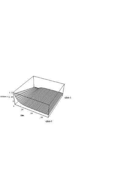
Figure 4: Graph of effective fitness as a function of time for the one-locus model of section 4.

In this case, $f=2$, $p_{1}=0.15$, $p_{2}=0.1$ and $P(0,0)=P(1,0)=0.5$. Note the significant differences in $f_{\scriptscriptstyle\rm eff}(i,0)$ as a result of which there is a population flow from $1$ to $0$ along this effective fitness gradient even though there is no reproductive fitness gradient. This gradient decreases monotonically as a function of time thus the effective landscape becomes flat asymptotically. We can see from (11) that this will be a generic property of any effective fitness landscape, the only steady state solutions of the equation being $f_{\scriptscriptstyle\rm eff}({\scriptstyle C}_{i},t)={\bar{f}}(t)\ \forall{\scriptstyle C}_{i}$, or $P({\scriptstyle C}_{i},t)=0$. Thus, already we see the usefulness of effective fitness — it indicates by its deviation from flatness how close the population is to a steady state.

For the two-locus model the reproductive fitnesses of $00$ and $01$ are equal. However, their effective fitnesses are quite different being: $f_{\scriptscriptstyle\rm eff}(00,0)=(1-0.9p+9.9p^{2})$ and $f_{\scriptscriptstyle\rm eff}(01,0)=(1+9p-9.9p^{2})$ respectively, where initial proportions of all four states are taken to be equal. The effective fitness landscape in this problem is shown in Figure 5 for $t=0$ with $p=0.05$, $P(00,0)=3$, $P(01,0)=0.2$, $P(10,0)=0.4$ and $P(11,0)=0.1$.

Figure 5: Graph of effective fitness at $t=0$ for the two-locus model of section 4.

Notice the initial effective fitness gradient from $00$ to $01$ that $\rightarrow 0$ as $t\rightarrow\infty$ as can be seen in Figure 6 which shows the same effective fitness landscape as in Figure 5 but at late times. Once again note the flatness of the effective landscape at late times.

Figure 6: Graph of effective fitness at late times for the two-locus model of section 4.

In the case of a strictly flat fitness landscape characteristic of neutral evolution the effective fitness is

$$f_{\scriptscriptstyle\rm eff}({\scriptstyle C}_{i},t)=f\sum_{j=1}^{2^{N}-1}{P({\scriptstyle C}_{j},t)\over P({\scriptstyle C}_{i},t)}p^{d_{ij}}(1-p)^{N-d_{ij}}$$ (14)

For a homogeneous population $f_{\scriptscriptstyle\rm eff}({\scriptstyle C}_{i},t)=f\forall{\scriptstyle C}_{i},t$. Thus, under these circumstances the effective fitness landscape is as flat as the normal one. Small deviations from homogeneity will be manifest in small corrugations of the effective fitness landscape which will gradually diminish as the population homogenizes. If the landscape only has a flat subspace the system will seek to escape the flat subspace by way of the direction with the highest effective fitness gradient.

In the case of the NIAH landscape the effective fitness of the optimum string is

$$f_{\scriptscriptstyle\rm eff}(C_{\scriptscriptstyle\rm opt},t)=f_{0}(1-p)^{N}$$

$$+f_{1}\sum_{{\scriptstyle C}_{i}\neq{\scriptstyle C}_{i}}{P({\scriptstyle C}_{i},t)\over P(C_{\scriptscriptstyle\rm opt},t)}p^{d_{ij}}(1-p)^{N-d_{ij}}$$ (15)

In Figure 7 we see a plot of the effective fitness as found in a simulation of the Eigen model in the steady state as a function of $p$. In this case $f_{0}=9$ and $f_{1}=1$.

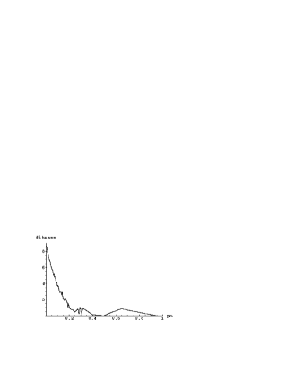
Figure 7: Graph of effective fitness versus $p$ in the steady state limit of the NIAH landscape.

For $p=0$, $f_{\scriptscriptstyle\rm eff}(C_{\scriptscriptstyle\rm opt},\infty)=f_{0}$ i.e. reproductive and effective fitness are the same. Note how the error threshold, located at about $0.2$, manifests itself in terms of the effective fitness — that at and above the threshold $f_{\scriptscriptstyle\rm eff}(C_{\scriptscriptstyle\rm opt},t)\rightarrow{\bar{f}}(t)\approx f_{1}$. i.e. once again the effective fitness landscape will be flat. The curve for $p>p_{\scriptscriptstyle\rm cri}$ is quite noisy due to the fact that there are very few optimum strings in the population. Thus, the effective fitness itself can serve as an order parameter to distinguish the selection dominated regime from the mutation dominated one.

Consider now the examples of section 5. In the first example, in Figure 8 we see the effective fitness as a function of time for the various two-schemata. Note the initial monotonic ordering of the schemata — the longest being the most effectively fit.

Figure 8: Graph of effective fitness versus time for the unitation model of Figure 1.

For the self-adaptive system if we concentrate for the moment on just selection and mutation the effective fitness of a given string is

$$f_{\scriptscriptstyle\rm eff}({\scriptstyle C}_{i},t)=f({\scriptstyle C}_{i},t)(1-p_{i})^{N}$$

$$+\sum_{{\scriptstyle C}_{i}\neq{\scriptstyle C}_{i}}p_{j}^{d_{ij}}(1-p_{j})^{N-d_{ij}}f({\scriptstyle C}_{i},t){P({\scriptstyle C}_{j},t)\over P({\scriptstyle C}_{i},t)}$$ (16)

where $p_{i}$ is the mutation rate associated with the genotype ${\scriptstyle C}_{i}$. To understand the behavior shown in Figure 2 we first realize that there are two contributions to $f_{\scriptscriptstyle\rm eff}({\scriptstyle C}_{i},t)$: one from the genotype ${\scriptstyle C}_{i}$ itself and another from all the other genotypes that can mutate to it. For the first contribution we can see that genotypes with low mutation rates will be preferred while for the second contribution genotypes with higher mutation rates will tend to be preferred. Thus, we can see a quantitative way of evaluating the explanation given in section 5. Initially, before the landscape jump, selection dominated in that the first term in (16) was the most important. Consequently the average mutation rate decreased as genotypes of low $p_{i}$ were more effectively fit. After the jump there is at first a preference for the local optimum at $40$, $41$. This is due to the fact that both terms in the effective fitness are playing an important role whereas for the needle-like global optimum, as the original population before the jump had converged to $10$, $11$, there was no contribution from the first term to $f_{\scriptscriptstyle\rm eff}(63,t)$. The fact that the average Hamming distance from $10$ and $11$ to $63$ is $3.5$, while from $10$, $11$ to $40$, $41$ it is $2.75$, explains why the system first converges to $40$, $41$ before passing on to the global optimum. It is clear too why the average mutation rate increases at two distinct points in the the search process. It is precisely when the second contribution in the effective fitness is playing a dominant role in aiding the search.

The giraffe example is rather similar to that of the self-adapting system, the master gene being analogous to the part of the genotype that codes for the mutation and recombination rates in the latter. It plays no role in reproductive selection but does play an important role in effective selection type one chromosomes having a higher effective fitness than type two during and after the drought.

All these examples show clearly how different the effective fitness landscape is from the reproductive fitness landscape and how population flows can be understood much better within the framework of the former.

7 Conclusions

In evolutionary computation, as in biology, it is obviously of crucial importance to know what generic properties the effective degrees of freedom exploited by a genetic system possess. Of particular concern is what constitutes a “fit” string. I have shown that in many situations high/low landscape reproductive fitness does not correspond to high/low effective fitness and it is the latter that really determines reproductive success.

Several criticisms of the effective fitness concept come immediately to mind. First of all, why do we need another type of landscape? Isn’t the present one good enough? After all, the notion of an adaptive landscape has turned out to be one of the most powerful concepts in evolutionary theory. One of the strongest motivations for the fitness landscape concept is that it allows one to intuitively understand population flows as hill climbing processes, thus offering a compelling paradigm for how evolution works. However, as I have demonstrated the hill climbing analogy is intimately linked to a certain type of dynamics associated with pure selection. In the presence of other genetic operators hill climbing is the exception rather than the norm and so the idea of a fitness landscape thereby loses some of its appeal. Another possible criticism is that effective fitness is intrinsically time-dependent. Doesn’t this lead to an extra level of complication relative to that of a static landscape? As I have argued there are several motivations for thinking of a time dependent landscape as being more fundamental than a static one. First of all, it is more biologically realistic as environmental effects that affect fitness are almost inevitably time dependent. Secondly, even if a landscape is static in terms of the microscopic degrees of freedom it will be time dependent in terms of any coarse grained degrees of freedom. On might also argue that the definition is tautological — survival of the survivors. Such circularity is not very different to that which appears in other sciences such as physics where one can level the same sort of criticism at an equation such as Newton’s Second Law. Such circularity is usually a hallmark of a truly fundamental concept and its definition. Additionally, in the present context we have a way to, at least in principle, explicitly compute it in terms of the parameters associated with the various genetic operators.

Another advantage of the effective fitness concept is that it allows one to quantitatively understand the different mechanisms by which order may arise in evolution. i.e. that “order” may arise due to the effect of genetic operators other than selection. In particular it provides a framework within which neutral evolution and natural selection can be understood as different sides of the same coin, and in particular under what circumstances neutral mutations may lead to adaptive changes. In this sense the phenomenon of orthogenesis, i.e. genetic drives in the presence of random mutations, is nothing more than the appearance of an effective fitness gradient in the case where there was no original reproductive fitness gradient. Clearly, much more work needs to be done in understanding the effective fitness concept and developing an intuition for landscape analysis based on it rather than the traditional idea of fitness landscape.

Acknowledgements

This work was partially supported through DGAPA-UNAM grant number IN105197. Many of the basic ideas presented here were developed in collaboration with Henri Waelbroeck to whom I am grateful for many stimulating conversations. I also wish to thank Sara Vera for help with the graphs and David Fogel for useful comments on the manuscript.

Bibliography

- [1] S. Wright, The roles of mutation, inbreeding, crossbreeding and selection in evolution, In: Jones DF (ed) Proceedings of the sixth international congress on genetics, vol 1, pp356-366, Brooklyn Botanic Garden, New York (1932).
- [2] S. A. Kauffman, The Origins of Order, Oxford University Press, Oxford (1993).
- [3] D.B. Fogel, Evolutionary Computation: The Fossil Record, IEEE Press (1998).
- [4] T.C. Jones, Evolutionary Algorithms, Fitness Landscapes and Search, Ph. D thesis Univ. of New Mexico (1995).
- [5] M. Eigen Self-Organization of Matter and the Evolution of Biological Macromolecules, Naturwissenschaften 58: 465 (1971).
- [6] J. Horn and D.E. Goldberg, Genetic Algorithm Difficulty and the Modality of Fitness Landscapes, FOGA 3, pp 243-271, eds D. Whitley and M.D. Vose, Morgan Kaufmann, San Francisco (1995).
- [7] K. Chellapilla, D.B. Fogel and S.S. Rao, Gaining Insight into Evolutionary Programming Through Landscape Visualization: An Investigation into IIR Filtering, Evolutionary Programming VI, eds. P.J. Angeline, R.G. Reynolds, J.R. McConnell and R. Eberhardt, Springer Verlag, Berlin (1997).
- [8] D.H. Ackley, An empirical study of bit vector optimization, Genetic algorithms and simulated annealing, pp 170-204, ed L. Davis, Pitman, London (1987).
- [9] R.A. Fisher, The Genetical Theory of Natural Selection, Clarendon Press, Oxford (1930).
- [10] P. Stadler, Towards a theory of landscapes, Complex Systems and Binary Networks, pp 77-155, eds R. López Peña et al, Springer (1995).
- [11] M.W. Strickberger, Evolution, Jones and Bartlett, Boston (1990).
- [12] J.D. Hofbauer and K. Sigmund, The Theory of Evolution and Dynamical Systems, Cambridge University Press (1992).
- [13] C.R. Stephens and H. Waelbroeck, Analysis of the Effective Degrees of Freedom in Genetic Algorithms, Physical Review E57, pp 3251-3264 (1998).
- [14] C.R. Stephens and H. Waelbroeck, Effective Degrees of Freedom of Genetic Algorithms and the Block Hypothesis, Proceedings of the Sixth International Conference on Genetic Algorithms, Morgan Kaufman, San Francisco, pp 34-41 (1997).
- [15] M. Kimura, The Neutral Theory of Molecular Evolution, Cambridge University Press, Cambridge (1983).
- [16] C.R. Stephens, H. Waelbroeck and R. Aguirre, Schemata as Building Blocks: Does Size Matter?, to be published in FOGA 5, eds. C. Reeves and W. Banzhaf, Morgan Kaufman, San Francisco (1999).
- [17] C.R. Stephens, I. García Olmedo, J. Mora Vargas and H. Waelbroeck, Self-Adaptation in Evolving Systems, Artificial Life 4.2, pp 183-201 (1998).
- [18] J. Mora, H. Waelbroeck, C.R. Stephens and F. Zertuche Symmetry Breaking and Adaptation: Evidence From a Simple Toy Model of a Viral Neutralization Epitope, National University of Mexico Preprint ICN-UNAM-97-10 (adap-org/0797) to be published in Biosystems (1997).
- [19] I. Leutheusser, J. Chem. Phys. 84, pp. 1884 (1986).