On thermostats and entropy production

Abstract

The connection between the rate of entropy production and the rate of phase space contraction for thermostatted systems in nonequilibrium steady states is discussed for a simple model of heat flow in a Lorentz gas, previously described by Spohn and Lebowitz. It is easy to show that for the model discussed here the two rates are not connected, since the rate of entropy production is non-zero and positive, while the overall rate of phase space contraction is zero. This is consistent with conclusions reached by other workers. Fractal structures appear in the phase space for this model and their properties are discussed. We conclude with a discussion of the implications of this and related work for understanding the role of chaotic dynamics and special initial conditions for an explanation of the Second Law of Thermodynamics.

I Introduction

There has been an intense interest over the past several years in the properties of fluid systems subjected to Gaussian thermostats. These thermostats are fictitious reversible force fields added to the equations of motion for fluid systems, and were introduced by people doing molecular dynamics simulations on fluids in stationary nonequilibrium systems in order to prevent the fluids from heating up indefinitely[1, 2]. These thermostatted systems have attracted the attention of workers in statistical mechanics and in dynamical systems theory for a variety of reasons: Firstly, since phase space volumes are not conserved in systems with Gaussian thermostats, and since the irreversible entropy production in systems subjected to these type of thermostats can be equated to the average rate of contraction of phase space volume on a microscopic scale, it follows that the rate of entropy production is equal to the negative of the sum of all Lyapunov exponents in the system [1, 2, 3]. Secondly, if, as often is the case, the irreversible entropy production may also be expressed in terms of transport coefficients and thermodynamic driving forces, there is a direct link between dynamical systems properties and nonequilibrium statistical mechanics for such systems. Thirdly, a point of great interest is that the phase space contraction induced by Gaussian thermostats in macroscopically stationary nonequilibrium states causes these states to live on fractal attractors that can be characterized by Sinai-Ruelle-Bowen (SRB) measures. Gallavotti, Cohen and Ruelle[4] have conjectured that these may be the generic type of states needed to describe stationary nonequilibrium states. Their Kaplan-Yorke dimension, which is related directly to sums of Lyapunov exponents, also measures the irreversible entropy production as recently discussed by Evans et al.[5], in a way similar to that described by Gaspard for Hamiltonian systems with escape[7]. Finally, Ruelle has argued[8] that in a stationary state on a compact subset of phase space, such as a shell of constant kinetic energy, the average rate of phase space contraction cannot be negative, since the phase space volume occupied by the state cannot expand without bounds. Therefore the irreversible entropy production cannot be negative, which would demonstrate the validity of the Second Law of thermodynamics for Gaussian thermostated systems.

In order to avoid having fictitious Gaussian thermostats acting everywhere in the system, Chernov and Lebowitz[9] studied a different class of thermostats that are active only at the boundaries of the system. These thermostats act in such a way that no energy is exchanged between thermostat and system, but the velocity distribution of the particles reflected from the walls of the system is contracted in such a way that a stationary shear flow results, giving rise to an irreversible entropy production. In the infinite system limit the shear induced irreversible entropy production could be equated again to the average rate of phase space contraction produced by the thermostat, but other cases no such relation existed for finite systems clear deviations from this equality were found. Obviously this could be due either to irreversible entropy production in kinetic modes, which are always present in boundary layers, or to a a complete breakdown of the relation between phase space contraction rate and irreversible entropy production. Related results have also been obtained by Klages and coworkers[10]. These authors have constructed a variety of thermostats which act only during collisions of particles with fixed scatterers or walls, and also lead to nonequilibrium steady states, with phase space contraction onto a lower dimensional attractor. In these models, the entropy production may or may not be related to the rate of phase space contraction, depending upon the precise nature of the thermostat and the system.

Here we will show on the basis of a simple and fairly natural example that indeed one can find thermostats for which the relation between the rate of phase space contraction and the rate of entropy production breaks down, and, in addition, we show one may have stationary nonequilibrium states without an overall phase space contraction, as previously shown by Gaspard[11]. Our model consists of a Lorentz gas enclosed between walls at different temperatures, a system for which Spohn and Lebowitz proved long ago[12] that it satisfies Fourier’s law of heat conduction in the Grad limit, in which one sends the size of the scatterers to zero while increasing their density in such a way that the ratio between mean free path and system size remains constant. The support of the stationary measure will have the same dimension as the full phase space, yet it will exhibit strong fractal features in the form of a fractal repeller located on the boundary between two subsets of different energy, very similar to the fractal boundaries studied by Gaspard in the framework of particle diffusion [11]. The Lyapunov exponents of the system will turn out to be simply related to those of the equilibrium system. Finally we will comment on the consequences of our considerations for the Second Law. We will argue that the assumptions used to obtain this law in our context may be replaced by other, equally reasonable, assumptions which lead to violations of the Second Law.

II The Lorentz gas

The system considered here is the usual Lorentz gas consisting of fixed spherical scatterers located at random positions in a $d$-dimensional space, and a light point particle moving between the scatterers at constant speed and making specular, elastic collisions with them. We will assume that the scatterers cannot overlap each other so as to avoid some problems with ergodicity and percolation that may occur in the case of overlapping scatterers. Instead of this choice we could also consider periodic billiards, with scatterers arranged on a regular lattice (preferably without infinite horizons), or systems with randomly oriented polyhedral scatterers instead of spherical ones. In the latter case all Lyapunov exponents would be trivially zero, but, as in the case of the periodic billiards, the transport properties would hardly differ from those of the ordinary Lorentz gas[13]. As boundaries we choose two parallel flat walls, separated by a distance $L$. The system may be infinite or periodically repeated in the directions parallel to the walls. The collisions of the light particle with these walls are also specular in direction, but the speed with which the particle leaves a wall will always be uniformly distributed in the range $v_{i}(1-\epsilon/2)\leq v\leq v_{i}(1+\epsilon/2),i=1,2,$ where $\epsilon<<1$, and $v_{1}=(dk_{B}T_{1}/m)^{1/2}$ is the average speed for one wall and $v_{2}=(dk_{B}T_{2}/m)^{1/2}$, for the other. Eventually we have in mind the limiting case where $\epsilon$ tends to zero. Further, $m$ is the mass of the light particle, $T$ is temperature, $k_{B}$ Boltzmann’s constant and $d$ the dimensionality. We suppose that the scatterers are distributed in space with number density $n$, and that they have radius $a$.

Spohn and Lebowitz[12] have shown rigorously that in the Grad limit, $n\rightarrow\infty,a\rightarrow 0,$ with $0<na^{d-1}<<1$, combined with the limit of $L$ tending to infinity, this system satisfies Fourier’s law of heat conduction: the temperature profile becomes linear and the energy current through the system becomes proportional to the temperature gradient. In addition, the coefficient of heat conduction can be obtained from the Lorentz-Boltzmann equation in this limit. One expects these results to hold much more generally in the limit of large L, except that for higher densities of scatterers (measured in dimensionless units $\tilde{n}=na^{d}$, with $\tilde{n}>0$) the transport coefficient will not be following from the Lorentz-Boltzmann equation any more.

III Entropy production and dynamical properties

It is easy to find an expression for the irreversible entropy production for these systems. As is usual for stationary thermostated systems[14] one has to argue that the irreversible entropy production per unit time has to equal the rate of entropy flow from the system into the thermostats. In the stationary state the average energy current through the system has to have a constant value $j_{e}$, so the average total entropy production per unit time $\sigma$ satisfies

$$\sigma=j_{e}(\frac{1}{T_{2}}-\frac{1}{T_{1}}),$$ (1)

where we assume $T_{1}>T_{2}$. In the present model it follows immediately that the energy current is directed from higher to lower temperature, as every time a particle changes its velocity from $v_{1}$ to $v_{2}$ it transfers an amount of energy $dk_{B}(T_{1}-T_{2})/2$ to the cold reservoir, whereas in changes from $v_{2}$ to $v_{1}$ it extracts the same amount of energy from the hot reservoir. It is not hard making explicit estimates of $j_{e}$, especially for small values of $\tilde{n}$, but for our present purposes it suffices that this current is non-zero. The phase space density of the particles traveling in the small range of speeds about $v_{i}$ is easily seen to be proportional to $v_{i}^{-(d+1)}$. This ensures, among other things, that the number of particles incident on a small area of the wall per unit time is equal to the number of particles leaving the small area per unit time. Furthermore, under the action of the thermostats as defined above there is no net contraction of phase space density. Indeed on a collision reducing $v_{1}$ to $v_{2}$ the phase space density at the coordinates of the collision is multiplied by a factor $(v_{1}/v_{2})^{(d+1)}$, but on the next collision bringing the speed back to $v_{1}$ this contraction is undone exactly and therefore the average rate of phase space contraction over a long time becomes exactly zero. As a result the identity between average phase space contraction rate and irreversible entropy production that holds for Gaussian thermostats, is not valid in the present case. In addition, the presence of a stationary heat current influences the Lyapunov exponents in a trivial way only. The crucial observation here is to note that the trajectories of the light particle are exactly the same as in equilibrium, only the parts of it that originate from the first wall are traversed at speed $v_{1}$ and those originating from the second wall with speed $v_{2}$. As a result the total time required for traversing a long trajectory is multiplied by a factor of $(1/v_{1}+1/v_{2})/(2/v)$ compared to the time needed by a particle with constant speed $v$. Hence all the Lyapunov exponents are multiplied by the inverse of this factor. The stationary measure on phase space is a measure with one constant density, proportional to $(1/v_{1})^{(d+1)}$ and restricted to the velocity range $v_{1}(1-\epsilon/2)\leq v\leq v_{1}(1+\epsilon/2)$, for points that can be traced back to a last collision with the first wall, and another constant density, proportional to $(1/v_{2})^{(d+1)}$ and confined to the velocity range $v_{2}(1-\epsilon/2)\leq v\leq v_{2}(1+\epsilon/2)$, for points coming from a last collision with the other wall. It is completely analogous to the measures considered by Gaspard to describe systems with a stationary diffusion current[11].

In spite of the absence of phase space contraction and the simplicity of the Lyapunov spectrum these stationary measures have strong fractal properties. Due to the way the model is constructed, the phase space trajectories for the moving particles are located on two thin energy shells about energies $mv_{i}^{2}/2,i=1,2$. In the stationary state, the trajectories on each shell are those whose last collision with a wall led to a value of the energy in the range of the shell. The trajectory of the particle may, of course, take place on both shells. To better visualize this phase space structure, it is helpful to rescale each of the energy shells so that they coincide. Under these circumstances, one may visualize the stationary state phase space regions as consisting of two disjoint subsets, separated by a boundary. Each of the subsets consists of points whose motion, extrapolated back in time reaches a particular wall. The boundary between these two subsets consists of points in phase space from which, extrapolating back in time, neither boundary is ever reached. An even smaller subset of this consists of points from which the boundaries are never reached either in the forward or in the backward time direction. This latter set is called a repeller, and it coincides with the intersection of its stable and unstable manifolds, that is, with the intersection of the set of points which may have collided with one or the other walls in the past but will not do so in the future (the stable manifold of the repeller), or have not collided with a wall in the past but may do so in the future (the unstable manifold of the repeller). Therefore, it is clear that the boundary of the two sets under discussion here coincides with the unstable manifold of the repeller.

The full fractal repeller described above plays a central role in the escape rate formalism of Gaspard and Nicolis[15]. In this formalism the escape rate from a system with open boundaries is related on the one hand to the diffusion coefficient, $D$, and on the other hand to the sum of positive Lyapunov exponents, $\lambda^{+}_{i}$  and the Kolmogorov-Sinai (KS) entropy, $h_{KS}$, on the repeller. For a Lorentz gas in two dimensions, Gaspard has shown how to express the partial information dimension, $d_{u}$, of the unstable manifold of the repeller to the diffusion coefficient of the moving particle in the fixed array of scatterers, and to the Lyapunov exponents and KS entropy[7]. In our case, this fractal dimension is given by

$$d_{u} = \frac{h_{KS}}{\lambda^{+}},$$ (2)

$$= 1-\frac{D\pi^{2}}{\lambda^{+}L^{2}}+o(L^{2}).$$ (3)

Simple scaling arguments show that this dimension is independent of the velocity of the particle on the unstable manifold, so that our scaling of the two energy shells to make them coincide does not affect the dimension of the boundary separating the two sets of phase points.

In the present system the coefficient of heat conduction may also be related to properties of the repeller. This follows from the work of Dorfman and Gaspard who derived a relation between the coefficient of heat conductivity and the dynamical properties of trajectories on an appropriate repeller for heat conduction[16]. This repeller is obtained by looking at the fluctuations of the Helfand moments associated with heat conduction. The Helfand moments undergo a deterministic diffusion in phase space. When the magnitude of the Helfand moment for a given trajectory in phase space exceeds a certain value, say $(d/2)k_{B}T|L/2|$, one considers that the system has “escaped” from a region in phase space, and the escape-rate formalism may be applied. In the case of the Lorentz gas under discussion here, the Helfand moments for heat flow and for diffusion are essentially the same, differing only by a constant factor, since the moving particle keeps a constant energy one collision with a wall to the next. until collIding with a wall. Thus the dimensional properties of the stable and unstable manifolds of the repellers are the same in both cases, diffusion and heat conductivity.

IV Discussion

The simple example discussed in this paper shows that macroscopically stationary nonequilibrium measures need not be phase space contracting and, consequentially, the average rate of irreversible entropy production need not be equal to the average rate of phase space contraction. In fact it seems to us that the thermostat considered here is closer to physical reality than the Gaussian thermostats that do give rise to the identities mentioned above. The net effect of our thermostat may be described as mimicking a transport of phase space density between the hot and the cold reservoir. As a result of this the temperatures of these reservoirs will approach each other (though very slowly if the reservoirs are really large) and the coarse grained entropy, based on a coarse grained phase space density, will decrease in the hot reservoir, but increase by a larger amount in the cold reservoir. This scenario can be made very plausible by probabilistic arguments, but is very hard to prove for almost any Hamiltonian model. Both Gaussian thermostats and the thermostat considered above can be considered as simplified models of real, Hamiltonian thermostats, in which the expected properties have been built in from scratch. It does not appear plausible though that in realistic systems coupled to thermostats at different temperatures the microscopic phase space density will keep increasing forever without bounds. In view of Liouville’s theorem physical changes in phase space density always must be the result of exchanges of phase space density between the system and its thermostats. If the latter may be treated as stationary sources the distribution of phase space density in a stationary nonequilibrium state for the system has to be stationary as well. In our opinion the feature of steady phase space contraction really is an artifact of Gaussian thermostats. This even raises the question whether there is a real use for these besides their handiness in nonequilibrium steady state simulations, but there certainly is. First of all Gaussian thermostats can be used as dynamical probes of nonequilibrium properties, precisely because of their satisfying the equality of entropy production and phase space contraction rate. Further, there are strong indications that at least for systems not too far from equilibrium, Gaussian thermostats lead to behavior that is almost indistinguishable from that brought about by more physical thermostats[1, 17, 18]. The nonequilibrium features of stationary nonequilibrium measures show up predominantly in their fractal features. The latter are much more visible for systems with Gaussian thermostats, in which the stationary measure lives on a fractal exclusively, than in the presumably more physical stationary measures in which the fractal features only show up in the boundaries between subsets with different densities. Therefore systems with Gaussian thermostats may be more suitable in the end for a dynamical study of nonequilibrium states. At this moment it is unclear whether this really is the case and in addition the relations between systems with different types of thermostats still largely have to be established.

We now make some remarks on the implications of thermostating mechanisms for the Second Law of thermodynamics. We indicated already that the generation of an average energy current from the hot to the cold reservoir has been built into our thermostat by hand. To make this point somewhat clearer, let us consider a somewhat more physical thermostat. As illustrated in Figure 1 it consists of a gas of particles that do not see the Lorentz gas walls, but instead are confined by a wall somewhat inside the Lorentz gas region. The latter wall in turn is invisible to the light Lorentz gas particle. In the narrow strip between these two walls the Lorentz gas particle may collide with the thermostat particles and so, if these collisions are sufficiently frequent, the light particle will leave the strip with a kinetic energy that on average is proportional to the temperature of the thermostat.

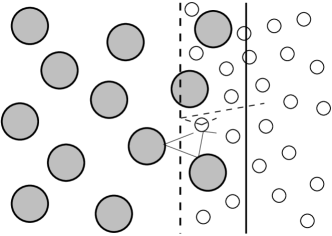
FIG. 1.: A more physical thermostat. This figure shows a small part of a boundary region of a Lorentz gas with a more pysical thermostat. The large circles are fixed scatterers and the small circles are moving thermostat particles. The solid line indicates the wall of the Lorentz gas, which is impenetrable to the light Lorentz gas particle but invisible to the thermostat particles. The dashed line indicates the wall of the thermostat, which is invisible to the Lorentz gas particles. The solid and dashed broken line describe part of a trajectory of the light Lorentz gas particle and a thermostat particle respectively.

The combined action of two of these thermostats on either side, with temperatures $T_{1}$ and $T_{2}$, will be basically the same as that of our simple model thermostats. For this to be true, however, we implicitly have to break time reversal symmetry by assuming that the velocity distributions of the Lorentz particle and of the thermostat particles before their collision are mostly uncorrelated, in other words we have to assume Boltzmann’s Stoszzahlansatz or some generalization of it. Instead, we could have required such property to hold after the collision [19]. This would correspond to the macroscopic arrow of time running in the opposite direction. Of course, we as observers would not notice the difference. Only an outside observer could notice our inversion of the notions of past and future. But, as remarked by e.g. Schulman[20], more exotic possibilities cannot be excluded. The arrow of time could run one way in parts of the system and the other way in other parts. Also, on the basis of known microscopic equations of motion one cannot exclude the possibility that at some time the direction of the macroscopic arrow of time will turn around, perhaps through growth of the area in which it runs the opposite way. To explain our obvious observation of a well defined direction of time, reversible microscopic equations simply do not suffice. Apparently we do need the additional fact that at some point in time our universe was brought into a state of extremely low entropy, so we observe an arrow of time moving away quite definitely from that point. And in spite of any lack of evidence we cannot exclude the possibility that the temporal boundary conditions to the ‘equations of motion of our universe’ are not all located in the past, which then might lead indeed to eventual inversions of the arrow of time. In view of this it seems clear that proofs of the Second Law will have to require additional information about the properties and the history of our universe and cannot be based exclusively upon the mixing or chaotic properties of the microscopic equations of motion, or on properties of thermostats in stationary nonequilibrium systems. In less cosmic language, we might say that some assumptions about the absence of initial correlations in our systems will have to be made in order to demonstrate the validity of the Second Law, no matter how chaotic the dynamics of our system. Along these lines, a much more modest goal, which is still very hard to attain, is to show that isolated systems showing sufficient lack of correlations initially, will indeed satisfy the Second Law. Here perhaps thermostats can be of some use, but in order to be credible, they would have to be of Hamiltonian type .

V Acknowledgements

For both of us Joel Lebowitz has been a dear friend for over thirty five years. It is a great pleasure being able to contribute to this very special Festschrift. We congratulate Joel on his seventieth birthday and express our hope he will continue for many more years being an inspiring example for all statistical physicists in all his scientific and humanitarian efforts. We thank Rainer Klages for some valuable remarks on the manuscript. JRD wishes to thank FOM for support of visits to the University of Utrecht, and the National Science Foundation (USA) for support under grants PHY-96-00428 and PHY-98-20824. HvB acknowledges support by FOM, SMC and by the NWO Priority Program Non-Linear Systems, which are financially supported by the ”Nederlandse Organisatie voor Wetenschappelijk Onderzoek (NWO)”.

REFERENCES

- [1] D. J. Evans and G. P. Morriss, Statistical Mechanics of Nonequilibrium Liquids, Academic Press, London, (1990).
- [2] W. G. Hoover, Computational Statistical Mechanics, Elsevier Science Publishers, Amsterdam, (1991).
- [3] J. R. Dorfman, An Introduction to Chaos in Nonequilibrium Statistical Mechanics, Cambridge University Press, Cambridge, (1999).
- [4] G. Gallavotti and E. G. D. Cohen,Dynamical Ensembles in Stationary States, J. Stat. Phys. 80, 931 (1995); Dynamical Ensembles in Nonequilibrium Statistical Mechanics, Phys. Rev. Lett. 74, 2694; D. Ruelle, Smooth Dynamics and New Theoretical Ideas in Non-equilibrium Statistical Mechanics, J. Stat. Phys. 95, 393, (1999).
- [5] D. Evans, E. G. D. Cohen, D. Searles, and F. Bonetto, Note on the Kaplan-Yorke Dimension and Linear Transport Coefficients, cond-mat/9911455.
- [6] B. L. Holian, W. G. Hoover and H. A. Posch, Phys. Rev. Lett. 59, 10 (1987)
- [7] P. Gaspard, Chaos, Scattering and Statistical Mechanics, Cambridge University Press, Cambridge, (1998); Sec. 6.2.4.
- [8] D. Ruelle, Positivity of Entropy Production in Nonequilibrium Statistical Mechanics, J. Stat. Phys. 85, 1, (1996); Entropy Production in Nonequilibrium Statistical Mechanics, Comm. Math. Phys. 189, 365 (1997).
- [9] N. I. Chernov and J. L. Lebowitz, Stationary Non-equilibrium Sates in Boundary Driven Hamiltonian Systems: Shear Flow, J. Stat. Phys. 86, 953, (1997).
- [10] C. Wagner, R. Klages, and G. Nicolis, Thermostating by Deterministic Scattering: Heat and shear flow, Phys. Rev. E 60, 1401, (1999); R. Klages, K. Rateitschak, and G. Nicolis, Thermostatting by Deterministic Scattering, chao-dyn/9812021; K. Rateitschak, R. Klages, and G. Nicolis, Thermostatting by deterministic Scattering: The periodic Lorentz gas, chao-dyn/9908013.
- [11] S. Tasaki and P. Gaspard, Fick’s Law and Fractality of Non-equilibrium Stationary States in a Reversible Multi-baker Map, J. Stat. Phys. 81, 935, (1995); P. Gaspard, Entropy Production in Open, Volume Preserving Systems, J. Stat. Phys. 89, 1215, (1997).
- [12] J. L. Lebowitz and H. Spohn,Transport Properties of the Lorentz Gas: Fourier’s Law, J. Stat. Phys. 19, 633 (1978).
- [13] P. and T. Ehrenfest, The Conceptual Foundations of the Statistical Approach to Mechanics, Cornell University Press, Ithaca, (1959); C. P. Dettmann, E. G. D. Cohen, and H. van Beijeren, Microscopic Chaos from Brownian Motion?, Nature 401, 875, (1999).
- [14] J. R. Dorfman and H. van Beijeren, Dynamical Systems Theory and Transport Coefficients: A survey with applications to Lorentz gases, Physica A 240, 12 (1997)
- [15] P. Gaspard and G. Nicolis, Transport Properties, Lyapunov Exponents and Entropy per Unit Time, Phys. Rev. Lett. 65, 1693 (1990); P. Gaspard and F. Baras, Dynamical Chaos Underlying Diffusion in the Lorentz Gas, in Microscopic Simulations of Complex Hydrodynamic Phenomena, p.301, M. Maréschal and B. Holian, eds., Plenum, New York, (1992).
- [16] J. R. Dorfman and P. Gaspard, Chaotic Scattering Theory of Transport and Reaction-Rate Coefficients, Phys. Rev. E51, 28, (1995).
- [17] D. J. Evans and S. Sarman, Equivalence of Thermostatted Nonlinear Responses, Phys. Rev. E 48, 65, (1993).
- [18] G. Gallavotti, Chaotic Dynamics, Fluctuations and Nonequilibrium Ensembles, CHAOS, 8, 384, (1998).
- [19] E. G. D. Cohen and T. H. Berlin, Note on the Derivation of the Boltzmann Equation from the Liouville Equation Physica, 26, 717, (1960).
- [20] L. S. Schulman, Time’s Arrow and Quantum Measurement, Cambridge University Press, Cambridge, (1997); Opposite Thermodynamic Arrows of Time, cond-mat/9911101.