Deformation of surfaces, integrable systems and Chern-Simons theory

Abstract

A few years ago, some of us devised a method to obtain integrable systems in (2+1)-dimensions from the classical non-Abelian pure Chern-Simons action via reduction of the gauge connection in Hermitian symmetric spaces. In this paper we show that the methods developed in studying classical non-Abelian pure Chern-Simons actions, can be naturally implemented by means of a geometrical interpretation of such systems. The Chern-Simons equation of motion turns out to be related to time evolving 2-dimensional surfaces in such a way that these deformations are both locally compatible with the Gauss-Mainardi-Codazzi equations and completely integrable. The properties of these relationships are investigated together with the most relevant consequences. Explicit examples of integrable surface deformations are displayed and discussed.

1 Introduction

Many authors have extensively studied the deep relations among completely integrable systems and the basic equations of the differential geometry, like the Frenet formulae defining curves embedded in ${\bf R}^{3}$, or their analogous for the surfaces, the Gauss-Weingarten (GW) equations, and the corresponding integrability conditions, i.e. the Gauss-Mainardi-Codazzi (GMC) equations (see for instance [1,2,3]). In these approaches the main idea is to add to a generic differential geometry setting certain auxiliary conditions, containing from the beginning the properties of the completely integrable systems.

A slightly different situation occurs in the study of the so-called Darboux system [4,5], which naturally arises in looking for classes of orthogonal curvilinear coordinates in Euclidean spaces and whose integrability has been detected in Ref. 6. Such a system has been investigated mainly in connection with the Topological Field Theory [7]. On the other hand, some years ago some of us proposed a simple method to obtain completely integrable systems in ($2+1)$-dimensions, from classes of non Abelian Chern-Simons (CS) field theories, taking values in Hermitian symmetric spaces [8]. In this context completely integrable systems are seen as particular gauge choices in which the theory is formulated. Moreover, linear spectral problems are naturally related to the geometrical constraints imposed on the target space. From this point of view, integrable systems arise as special reductions, which break the general covariance and the gauge invariance of the original field theory, but preserve a residual symmetry in order to allow the Lax representation and the complete integrability, although the solvability is lost.

In the present work we show that this approach can be naturally implemented by resorting to a geometrical interpretation of the completely integrable systems mentioned above. Precisely, we show as the CS equation of motion can describe time evolving 2-dimensional surfaces in such a way that the deformation is not only locally compatible with the GMC equation, but completely integrable as well. The nature and the properties of such relationships are investigated together with the most important consequences. Furthermore, explicit examples of integrable deformations of surfaces are displayed.

The paper is organized as follows. Section 2 contains some results on the CS theory. In Section 3 the fundamental terminology and notations related to the theory of 2-dimensional surfaces are reviewed. In Section 4 the general formulation of deformation of 2-dimensional surfaces is presented. Section 5 is devoted to the analysis of certain spin models in (2+1)-dimensions. Section 6 is addressed to the bilinear representations of the spin systems fields and of the trihedral moving frame. Sections 7 and 8 concern with the deformations of surfaces from integrable (2+1)-dimensional spin systems and equations of the nonlinear Schrödinger type, respectively. In Sections 9 and 10 some solutions and special surfaces associated with spin system vortices are considered. Finally, in Section 11 some concluding remarks are reported.

2 Chern-Simons theory and completely integrable systems

Here we shall review some preliminaries concerning the CS theory and we show how one can connect them to the completely integrable systems in 2+1 dimensions. We are dealing with the field theory defined by the action

$$S\left[J\right]=\frac{k}{4\pi}\int_{M}Tr\left(J\wedge dJ+\frac{2}{3}J\wedge J\wedge J\right),$$ (1)

where $J$ is a 1-form gauge connection taking values in a simple Lie algebra $\hat{g}$ on an oriented closed three-manifold $M$, and $k$ is a coupling constant which should be quantized in a quantum theory [9]. The related classical equation of motion is the zero - curvature condition

$$F\equiv dJ+J\wedge J=0.$$ (2)

The action (1) is manifestly invariant under general coordinate transformations (preserving orientation and volumes). Moreover, under a generic gauge map $G:{M}\rightarrow{\ }\widehat{{G}}$ the gauge connection transforms as $J\rightarrow G^{-1}JG+G^{-1}dG$ . Correspondingly, the action (1) changes as $S[J]\rightarrow S[J]+2\pi\,k\,W(G),$ where

$$W(J)={\frac{1}{24\pi^{2}}}\int_{{M}}{Tr}(G^{-1}dG\wedge G^{-1}dG\wedge G^{-1}dG)$$ (3)

is the winding number of the map $G$ and takes integer values, because of the result $\pi_{3}(\widehat{{G}})={\bf Z}$ from the homotopy theory [10]. This is a Topological Field Theory in the sense that it possesses quantum observables, which are independent of the metric and are related to the Jones polynomials of the knot theory [11]. From other points of view, the action (1) has been used as an effective interaction for quasi-particles and vortices in two space dimensional systems, of interest in the physics of high temperature superconductivity [12], and in the context of the low dimensional gravity models (see [13] and reference therein). In the static self-dual reductions the system of equations (2) becomes the two - dimensional Toda field theory [14], the static reductions of the Ishimori model or of the Davey - Stewartson equation [15].

In [8] the general action (1) was reduced assuming that the Lie algebra $\hat{g}$ admits a ${\bf Z}_{2}$ graduation, in such a way the form $J$ splits in two parts, taking values on an isotropy subalgebra and a complement linear space, respectively. The former component will play the role of a gauge field with the isotropy group as a gauge group, the latter could be considered as a sort of coupled ”matter” field. At any point of the corresponding coset space we can introduce in a natural way a Riemannian torsion free connection [10]. Furthermore, the 3-manifold $M$ is trivialized into $\Sigma\times{\bf R}$, where $\Sigma$ is a Riemann surface, endowed with a set of local complex coordinates $z=x^{1}+ix^{2},$ and ${\bf R}$ is interpreted as the time axis. Thus the connection $J$ can be further decomposed into time and space-like components. In the simplest $SU\left(2\right)/U(1)\sim CP^{1}\sim S^{2}$ case the connection takes the form

$$J=\left(\begin{array}[]{ll}iv_{\mu}&-q_{\mu}^{\ast}\\ q_{\mu}&-iv_{\mu}\end{array}\right)dx^{\mu},$$

which can be rewritten in terms of complex forms

$$vdz=\frac{1}{2}\left(v_{1}-iv_{2}\right)dz,\quad\psi_{-}dz=\frac{1}{2}\left(q_{1}-iq_{2}\right)dz,\quad\psi_{+}d\overline{z}=\frac{1}{2}\left(q_{1}+iq_{2}\right)d\overline{z}.$$

This allows us to write the action (1) as follows

$$S=-\frac{k}{\pi}\int_{\Sigma\times{\bf R}}\{\frac{1}{2}\varepsilon^{\lambda\mu\nu}v_{\lambda}\partial_{\mu}v_{\nu}+\frac{i}{2}(\psi_{+}^{\ast}D_{0}\psi_{+}-\psi_{+}(D_{0}\psi_{+})^{\ast}-\psi_{-}^{\ast}D_{0}\psi_{-}+\psi_{-}(D_{0}\psi_{-})^{\ast})$$

$$-iq_{0}^{*}(D\psi_{+}-\stackrel{{\scriptstyle\_}}{{D}}\psi_{-})+iq_{0}(D\psi_{+}-\stackrel{{\scriptstyle\_}}{{D}}\psi_{-})^{*}\}dx^{0}dx^{1}dx^{2},$$ (4)

where $D_{0}=\partial_{0}-2iv_{0}$, $D=\partial_{z}-2iv$, $\overline{D}=\partial\overline{{}_{z}}-2iv^{\ast}$ (^∗ denotes the complex conjugation). The first order Lagrangian involved in (4) is constrained by the torsion-free condition

$${D}\psi_{+}-{\bar{D}}\psi_{-}=0$$ (5)

and by what we call the Gauss - Chern - Simons (GCS) law

$${\partial}_{z}{v}^{\ast}-{\partial}_{\overline{z}}v=-i\left({{\left|{{\psi}_{+}}\right|}^{2}-{\left|{{\psi}_{-}}\right|}^{2}}\right),$$ (6)

enforced by the Lagrangian multipliers $q_{0}$ and $v_{0}$, respectively. Of course, here we are looking in a different way to a subset of the equations of motion (2), in which the general covariance is broken. Indeed, only the isotropic $U(1)$ invariance is left. Furthermore, by exploiting the local isomorphism between $so(3)$ and $su(2)$ realized by the adjoint representation of the connection

$$J^{(ad)}=\left(\begin{array}[]{lll}0&-v_{0}&-Re(q_{0})\\ v_{0}&0&-Im(q_{0})\\ Re(q_{0})&Im(q_{0})&0\end{array}\right)dx^{0}+$$

$$\left(\begin{array}[]{lll}0&-2Re(v)&-Re(\psi_{+}+\psi_{-})\\ 2Re(v)&0&-Im(\psi_{+}+\psi_{-})\\ Re(\psi_{+}+\psi_{-})&Im(\psi_{+}+\psi_{-})&0\end{array}\right)dx^{1}+$$

$$\left(\begin{array}[]{lll}0&2Im(v)&-Im(\psi_{+}-\psi_{-})\\ -2Im(v)&0&-Re(\psi_{+}-\psi_{-})\\ Im(\psi_{+}-\psi_{-})&Re(\psi_{+}-\psi_{-})&0\end{array}\right)dx^{2},$$

we are able to introduce the so-called moving trihedral frame $\{{\bf e}_{i}\}$ in ${\bf R}^{3}$ [10], which satisfies the orthonormal conditions

$${\bf e}_{i}\cdot{\bf e}_{j}=\delta_{ij},\,\,\,{\bf e}_{i}\wedge{\bf e}_{j}=\varepsilon_{ijk}{\bf e}_{k}$$ (7)

and changes accordingly to

$$\partial_{\mu}{\bf e}_{i}=(J_{\mu})_{ik}^{(ad)}{\bf e}_{k},\quad\mu=0,1,2,\quad i=1,2,3.$$ (8)

Its integrability is assured by the zero curvature condition, namely by Eq. (2). For instance, assigning to ${\bf e}_{3}$ the special role of unimodular normal vector to a given surface ${\cal S}$, whose tangent plane is defined by the vectors $\left({\bf e}_{1},{\bf e}_{2}\right)$, the equations (8) for $\mu=1,2$ and $i=1,2,3$ can be seen as the Gauss-Weingarten equations of such a surface. Moreover, the mapping ${\bf e}_{3}:{\cal S}\longrightarrow S^{2}$ is the well known Gauss map. Furthermore, the corresponding integrability equations, rewritten as

$$\partial_{1}J_{2}^{\left(ad\right)}-\partial_{2}J_{1}^{\left(ad\right)}+\left[J_{1}^{\left(ad\right)},J_{2}^{\left(ad\right)}\right]=0,$$

are the Gauss-Codazzi-Mainardi equations for a surface $S$ immersed in ${\bf R}^{3}.$ They are the real form of the equations (5) and (6). The $U(1)$ invariance of such equations is readily interpreted as the invariance under local rotations of the tangent plane at the surface ${\cal S}$. This identification is one of the motivation of the present article and it will be fully developed from the geometrical point of view in the next Sections. Here we would like to show how to use effectively the remaining equations in (8) for $\mu=0$ and $i=1,2,3$ and the corresponding integrability conditions. In particular, we ask if structures related to the integrable systems can be detected in the above general picture. Then, since we show that it is the case, we are allowed to introduce a completely integrable dynamics for the trihedral frame and, by consequence, we can infer an integrable dynamics for the corresponding surfaces.

First, we can rewrite Eqs. (5) and (6) by introducing the quantities

$$V=\left(\begin{array}[]{ll}v*&\\ &v\end{array}\right),\quad\Psi_{\pm}=\left(\begin{array}[]{ll}&\psi_{\pm}\\ -\psi_{\pm}^{*}&\end{array}\right),\quad B=\frac{i}{2}\sigma_{3}\left(\Psi_{-}-\Psi_{+}\right).$$

Indeed, the torsionless condition (5) and its complex conjugate can be written as

$$\left(\begin{array}[]{ll}\partial_{z}&\\ &\partial_{\bar{z}}\end{array}\right)B+\frac{i}{2}\left(\partial_{\bar{z}}-\partial_{z}\right)\Psi_{-}+V\Psi_{-}-\Psi_{+}V=0,$$

while combining the GCS law (6) and its complex conjugate yields

$${\rm tr}\left\{\sigma_{3}\left[\left(\begin{array}[]{ll}\partial_{z}&\\ &\partial_{\bar{z}}\end{array}\right)V+B\Psi_{-}-\Psi_{+}B\right]\right\}=0.$$

These equations involve independent components in the basis of the complex $2\times 2$ matrices, and we have no information only about the identity component $\sigma_{0}$. So the last two equations provide

$$L_{+}\left[\frac{i}{2}\left(\partial_{\bar{z}}-\partial_{z}\right)+V+B\right]-\left[\frac{i}{2}\left(\partial_{\bar{z}}-\partial_{z}\right)+V+B\right]L_{-}=f\sigma_{0},$$ (9)

$$L_{\pm}=\left(\begin{array}[]{ll}\partial_{z}&\\ &\partial_{\bar{z}}\end{array}\right)-\Psi_{\pm}$$ (10)

has the form of the two-dimensional principal Zakharov-Shabat spectral problem [16] of elliptic type. Moreover, putting $f\equiv 0$ in equation (9), we obtain the so called space part of the Bäcklund transformations associated with $L_{\pm}$, defining the first-order Bäcklund-gauge operator

$$\hat{B}=\frac{i}{2}\left(\partial_{\bar{z}}-\partial_{z}\right)+V+B.$$

This means that $\hat{B}$ maps solutions of the two linear problems

$$L_{-}\phi_{-}=0\Rightarrow L_{+}B\phi_{-}=L_{+}\phi_{+}=0.$$ (11)

The previous considerations tell us that in the above formalism the Gauss - Codazzi - Mainardi equations are expressed in terms of products of first order differential operators, which have a precise meaning in the theory of the completely integrable systems. Of course, in this context an essential role is played by the second (evolution) linear operator of the Lax pair, in order to introduce a compatible time evolution. The latter, generally speaking, is non linear, while the corresponding equations from the CS theory still contains the arbitrary functions interpreted as Lagrangian multipliers in the action (4). Indeed, the corresponding equations read

$$D_{0}\psi_{+}=\bar{D}~{}q_{0},\qquad D_{0}\psi_{-}=D~{}q_{0},$$ (12)

$$\partial_{0}v-\partial_{z}v_{0}=i\left(q_{0}\psi_{+}^{\ast}-q_{0}^{\ast}\psi_{-}\right)$$ (13)

and their complex conjugated. However, we can exploit the freedom in the choice of $q_{0}$ and $v_{0}$ in order to fix the evolution of $\psi_{\pm}$ and $v$ in the $x^{0}$ variable. In fact, let us take

$$q_{0}=2i\left[\left(\bar{D}-\frac{i}{2}\left(\partial_{\bar{z}}\omega-i\partial_{\bar{z}}\chi\right)\right)\psi_{+}+\left(D-\frac{i}{2}\left(\partial_{z}\omega+i\partial_{z}\chi\right)\right)\psi_{-}\right],$$ (14)

where we require that the real functions $\chi$ and $\omega$ satisfy the supplementary conditions

$$\partial_{z}\partial_{\bar{z}}\chi=-4\left({{\left|{{\psi}_{+}}\right|}^{2}-{\left|{{\psi}_{-}}\right|}^{2}}\right),\quad\partial_{z}\partial_{\bar{z}}\omega=0.$$ (15)

Furthermore, by introducing an irrotational field ${\bf A}=\left(\partial_{z}\Lambda,\partial_{\bar{z}}\Lambda,\partial_{0}\Lambda\right)$ ( $\Lambda$ is an arbitrary real function) in such a way that

$$v=\frac{1}{4}\partial_{z}\Lambda-\frac{i}{8}\partial_{z}\chi,\quad v_{0}=\frac{1}{4}\left(\partial_{0}\Lambda+u_{0}\right),\quad\psi_{\pm}=\Psi_{\pm}\exp\left(\frac{i}{2}\Lambda\right),$$

the ”time evolutions” (12) become

$$i\partial_{0}\Psi_{\pm}+2\left(\partial_{z}^{2}+\partial_{\bar{z}}^{2}\right)\Psi_{\pm}+\frac{1}{2}u_{0}^{\pm}\Psi_{\pm}-i\left(\partial_{\bar{z}}\omega\partial_{\bar{z}}+\partial_{z}\omega\partial_{z}\right)\Psi_{\pm}=0,$$ (16)

where we have suitably defined in terms of $u_{0,}\chi$ and $\omega$ the scalar fields $u_{0}^{\pm}$ , which obey the consistency conditions arising from (13)

$$\partial_{z}\partial_{\bar{z}}u_{0}^{\pm}=8\left(\partial_{z}^{2}+\partial_{\bar{z}}^{2}\right)\left|\Psi_{\pm}\right|^{2}.$$ (17)

Thus, to summarize, the gauge fixing conditions (14) and (15) destroy the arbitraryness contained in the equations (12) in favour of a formally decoupled pair of Davey - Stewartson equations (16) and (17). Actually, between the two pairs of fields $\left(\Psi_{\pm},u_{0}^{\pm}\right)$ there still exists the coupling provided by the torsionless condition (5), which in the new variables takes the form

$$\left(\partial_{\bar{z}}+\frac{1}{4}\partial_{\bar{z}}\chi\right)\Psi_{-}=\left(\partial_{z}+\frac{1}{4}\partial_{z}\chi\right)\Psi_{+}.$$ (18)

As we discussed above, Eq. (18) is in essence the space part of the Bäcklund transformations. Starting from a known solution, say $\left(\Psi_{-},u_{0}^{-}\right)$ and fixing $\omega,$ one can reconstruct the function $\chi$, and solving (18) for $\Psi_{+},$ finally we find $u_{0}^{+}$ from (17). Furthermore, we observe that the gauge choice (14) - (15) is equivalent to fix the second operator of the Lax pair, denoted here by $M_{\pm}=\partial_{x^{0}}+\Sigma_{k=0}^{2}M_{\pm}^{\left(k\right)}\left[\frac{i}{2}\left(\partial_{\bar{z}}-\partial_{z}\right)\right]^{2-k}$, where $M_{\pm}^{\left(k\right)}$ are specific matrices. $M_{\pm}$ provide the system (16) - (17) and (18) by the compatibility relations

$$\left[L_{\pm},M_{\pm}\right]=0,\quad M_{+}\hat{B}-\hat{B}M_{-}=0.$$

Moreover, by using a suitable particular eigenfunction $\phi_{-}^{0}$ of the equation (11), it is well known (see [17],[18]) that one can construct a new spectral problem of the form

$$L_{-}^{I}=\left(\phi_{-}^{0}\right)^{-1}L_{-}\phi_{-}^{0}=\partial_{x^{1}}+iS\partial_{x^{2}},\quad M_{-}^{I}=\left(\phi_{-}^{0}\right)^{-1}M_{-}\phi_{-}^{0},$$

where

$$S=i\left(\phi_{-}^{0}\right)^{-1}\sigma_{3}\phi_{-}^{0}$$

is an element of $SU\left(2\right)/U\left(1\right)$ coset space and the corresponding eigenfunction is $\phi_{-}^{I}=\left(\phi_{-}^{0}\right)^{-1}\phi_{-}.$ The resulting integrable system is known as Ishimori model and it describes the evolution of a classical spin in a background generated by the density of the topological charge. Since this equation will be discussed in the next Sections, we do not give other details about it. But here we want to stress that such a system is an alternative integrable restriction of the possible configurations of the CS field, exactly as the Davey-Stewartson equation does. Furthermore, one can put the question if the spin field $S$ has something to do with the trihedral frame introduced above. The consequences arising from the identification of $S$ with one of the unimodular vector fields ${\bf e}_{i}$ is the main subject of the next Sections.

3 Surfaces in $R^{3}$

To introduce our terminology and notations and to make the exposition self-contained, we recall some basic facts from the theory of 2-dimensional surfaces. So, we consider a smooth surface in a three dimensional Euclidean space ${\bf R}^{3}$. Let $x,y$ be the local coordinates on the surface. At the same time, the surface can be described by the position vector ${\bf r}(x_{1},x_{2},x_{3})={\bf r}(x,y)$, where $x_{i}$ are coordinates of ${\bf R}^{3}$. The surface is uniquely defined within rigid motions by the two fundamental forms

$$I=Edx^{2}+2Fdxdy+Gdy^{2}$$ (19)

and

$$II=Ldx^{2}+2Mdxdy+Ndy^{2},$$ (20)

where $E,F,G,L,M,N$ can be defined by

$$E={\bf r}_{x}\cdot{\bf r}_{x}=g_{11},\quad F={\bf r}_{x}\cdot{\bf r}_{y}=g_{12}=g_{21},\quad G={\bf r}_{y}\cdot{\bf r}_{y}=g_{22},$$ (21)

$$L={\bf n\cdot}{\bf r}_{xx}=b_{11},\quad M={\bf n\cdot}{\bf r}_{xy}=b_{12}=b_{21},\quad N={\bf n\cdot}{\bf r}_{yy}=b_{22}.$$ (22)

In Equations (21) and (22)

$${\bf n}(x,y)=\frac{{\bf r}_{x}\wedge{\bf r}_{y}}{\mid{\bf r}_{x}\wedge{\bf r}_{y}\mid}=\frac{{\bf r}_{x}\wedge{\bf r}_{y}}{\sqrt{g}}\quad$$ (23)

is introduced, where $g=det(g_{ij})=EG-F^{2}=\mid{\bf r}_{x}\wedge{\bf r}_{y}\mid^{2},$ is the normal vector field at each point of the surface. Then the triple $({\bf r}_{x},{\bf r}_{y},{\bf n})$ represents a local frame of ${\bf R}^{3},$ the changes of which are characterized by the GW equations

$${\bf r}_{xx}=\Gamma_{11}^{1}{\bf r}_{x}+\Gamma_{11}^{2}{\bf r}_{y}+L{\bf n,}$$ (24)

$${\bf r}_{xy}=\Gamma_{12}^{1}{\bf r}_{x}+\Gamma_{12}^{2}{\bf r}_{y}+M{\bf n},$$ (25)

$${\bf r}_{yy}=\Gamma_{22}^{1}{\bf r}_{x}+\Gamma_{22}^{2}{\bf r}_{y}+N{\bf n,}$$ (26)

$${\bf n}_{x}=p_{11}{\bf r}_{x}+p_{12}{\bf r}_{y},$$ (27)

$${\bf n}_{y}=p_{21}{\bf r}_{x}+p_{22}{\bf r}_{y},$$ (28)

where the Christoffel symbols of the second kind are defined by $g_{ij}$ ( $g^{ij}=(g_{ij})^{-1})$ as

$$\Gamma_{jk}^{i}=\frac{1}{2}g^{il}(\frac{\partial g_{lk}}{\partial x^{j}}+\frac{\partial g_{jl}}{\partial x^{k}}-\frac{\partial g_{jk}}{\partial x^{l}}),$$ (29)

and

$$p_{ij}=-b_{ik}g^{kj}.$$ (30)

The principal curvatures $k_{1},k_{2}$ are the eigenvalues of the Weingarten operator

$$\Lambda=\left(\begin{array}[]{cc}E&F\\ F&G\end{array}\right)^{-1}\left(\begin{array}[]{cc}L&M\\ M&N\end{array}\right).$$ (31)

which for the mean and the Gassian curvature implies

$$H=\frac{k_{1}+k_{2}}{2}=tr(\Lambda)=\frac{EN+LG-2MF}{2(EG-F^{2}},$$ (32)

$$K=k_{1}k_{2}=det(\Lambda)=\frac{LN-M^{2}}{EG-F^{2}}.$$ (33)

One of the global characteristics of surfaces is the integral curvature

$$\chi=\frac{1}{2\pi}\int K\sqrt{g}dxdy,$$ (34)

which for compact oriented surfaces is the integer

$$\chi=2(1-\triangle),$$ (35)

where $\triangle$ is the genus of the surface. The compatibility conditions of the GW equations (24)-(28) furnish the GMC equations

$$R_{ijk}^{l}=b_{ij}b_{k}^{l},\quad\frac{\partial b^{ij}}{\partial x^{k}}-\frac{\partial b_{ik}}{\partial x^{j}}=\Gamma_{ik}^{s}b_{js}-\Gamma_{ij}^{s}b_{ks},$$ (36)

where $b_{i}^{j}=g^{jl}b_{il}$ and the curvature tensor is

$$R_{ijk}^{l}=\frac{\partial\Gamma_{ij}^{l}}{\partial x^{k}}-\frac{\partial\Gamma_{ik}^{l}}{\partial x^{j}}+\Gamma_{ij}^{s}\Gamma_{ks}^{l}-\Gamma_{ik}^{s}\Gamma_{js}^{l}.$$ (37)

For our purposes it is convenient to employ the triad of orthonormal vectors

$${\bf e}_{1}=\frac{{\bf r}_{x}}{\sqrt{E}},\quad{\bf e}_{2}={\bf n},\quad{\bf e}_{3}={\bf e}_{1}\wedge{\bf e}_{2}.$$ (38)

In terms of these vectors the GW equations (24)-(28) take the form

$${\bf e}_{jx}={\bf X}\wedge{\bf e}_{j},\quad{\bf e}_{jy}={\bf Y}\wedge{\bf e}_{j},$$ (39)

where

$${\bf X}=\tau{\bf e}_{1}+\sigma{\bf e}_{2}+k{\bf e}_{3},\quad{\bf Y}=m_{1}{\bf e}_{1}+m_{2}{\bf e}_{2}+m_{3}{\bf e}_{3},$$ (40)

and

$$k=\frac{L}{\sqrt{E}},\quad\sigma=\frac{2EF_{x}-EE_{y}-FE_{x}}{2E\sqrt{g}},\quad\tau=\frac{ME-LF}{\sqrt{gE}},$$ (41)

$$m_{1}=\frac{NE-MF}{\sqrt{gE}},\quad m_{2}=\frac{FE_{y}-EG_{x}}{2E\sqrt{g}},\quad m_{3}=\frac{M}{\sqrt{E}}.$$ (42)

Similarly, we can rewrite the GMC equations (32) in the following form

$$A_{y}-B_{x}+[A,B]=0,$$ (43)

with

$$A=\left(\begin{array}[]{ccc}0&k&-\sigma\\ -k&0&\tau\\ \sigma&-\tau&0\end{array}\right),\quad B=\left(\begin{array}[]{ccc}0&m_{3}&-m_{2}\\ -m_{3}&0&m_{1}\\ m_{2}&-m_{1}&0\end{array}\right).$$ (44)

Then, the GMC equation turns out to be equivalent to the set of equations for the coefficients of the first and second fundamental forms. This system, which is in general non integrable, reduces to integrable partial differential equations for certain particular surfaces [10].

4 Deformations of surfaces in 2+1 dimensions: the general formulation

It is well known that in some cases deformations of surfaces can be associated with integrable equations [1-3]. Here we are interested in the deformation of the two-dimensional surfaces discussed in Section 3. In other words, we have to deal with the motion of such surfaces. To this aim, let us introduce the vector field

$${\bf r}_{t}=a_{1}{\bf r}_{x}+a_{2}{\bf r}_{y}+a_{3}{\bf n},$$ (45)

where the $a_{i}$’s are some real functions. It is easy to show that the evolution of the local trihedral frame is given by

$${\bf e}_{jt}={\bf T}\wedge{\bf e}_{j},$$ (46)

$${\bf T}=\omega_{1}{\bf e}_{1}+\omega_{2}{\bf e}_{2}+\omega_{3}{\bf e}_{3},$$ (47)

$\omega_{j}$’s being real functions. Summarizing, the changes of the local frame are provided by

$${\bf e}_{jx}={\bf X}\wedge{\bf e}_{j},\quad{\bf e}_{jy}={\bf Y}\wedge{\bf e}_{j},\quad{\bf e}_{jt}={\bf T}\wedge{\bf e}_{j},$$ (48)

where the vectors X and Y are defined by (40). This system is analogous to the system (8) in Section 2.

The system (52) represents the simplest form of the (2+1)-dimensional GW equations.

By introducing the matrix

$$C=\left(\begin{array}[]{ccc}0&\omega_{3}&-\omega_{2}\\ -\omega_{3}&0&\omega_{1}\\ \omega_{2}&-\omega_{1}&0\end{array}\right)$$ (49)

and using the matrices $A$ and $B$ (see (44)), the compatibility conditions of Eqs. (48) entail

$$A_{y}-B_{x}+[A,B]=0,$$ (50)

$$A_{t}-C_{x}+[A,C]=0,$$ (51)

$$B_{t}-C_{y}+[B,C]=0.$$ (52)

Of the nine funcions $k,\sigma,\tau,m_{i},\omega_{i}$ involved in $A,B$ and $C$ only three are independent. In fact, we can express the functions $m_{i},\omega_{i}$ in terms of $k,\sigma,\tau$ and their derivatives. This point will be discussed later.

4.1 Some geometrical invariants and integrals of motion as consequence of the geometrical formalism

The formalism developed above yields some important invariants having a pure geometrical nature. Indeed, in terms of the triad vectors these geometrical invariants take the form

$$K_{1}^{(t)}=\int{\bf e}_{1}\cdot({\bf e}_{1x}\wedge{\bf e}_{1y})dxdy,\quad K_{2}^{(t)}=\int{\bf e}_{2}\cdot({\bf e}_{2x}\wedge{\bf e}_{2y})dxdy,\quad$$

$$K_{3}^{(t)}=\int{\bf e}_{3}\cdot({\bf e}_{3x}\wedge{\bf e}_{3y})dxdy.$$ (53)

In a similar way we can write down other two classes of invariants with respect to $x$ and $y$ directions, respectively. These geometrical invariants can be interpreted as ”topological charges”. However, three of them, namely $K_{i}^{(t)}$ $(i=1,2,3)$ behave as integrals of motion of the (2+1)-dimensional geometrical models under consideration. This will be elucidated in the next Sections. These invariants can be related to the topological Chern index of a curvature 2-form on a 2-dimensional space [19].

5 Integrable spin models in (2+1)- dimensions

Now let us dwell upon the problem of finding or building up integrable deformations of (2+1)-dimensional surfaces. Among several possibilities, within the geometrical formalism previously presented we shall consider multidimensional integrable spin (field) systems (MISSs) to recognize integrable deformations of surfaces.

5.1 The spin model

A few words on MISSs. At present there exist many integrable spin systems in (2+1)-dimensions (see, for example, Refs. [20,21-25]). A well known prototype of these systems is the Ishimori model (IM) [20]. A more general (2+1)-dimensional integrable spin model is described by the pair of equations

$${\bf S}_{t}+{\bf S}\wedge\{(b+1){\bf S}_{\xi\xi}-b{\bf S}_{\eta\eta}\}+bu_{\eta}{\bf S}_{\eta}+(b+1)u_{\xi}{\bf S}_{\xi}=0,$$ (54)

$$u_{\xi\eta}={\bf S\cdot}({\bf S}_{\xi}\wedge{\bf S}_{\eta}),$$ (55)

where $\xi,\eta$ are real or complex variables, $b$ is a real constant, ${\bf S}=(S_{1},S_{2},S_{3})$ is the spin (field) vector, ${\bf S}^{2}=1$, and $u$ is a scalar function. These equations, which are called M-XX equations (about our conditional notations, see e.g. [21-25]), are one of the (2+1)-dimensional integrable generalizations of the isotropic Landau-Lifshitz (LL) equation

$${\bf S}_{t}={\bf S}\wedge{\bf S}_{xx}.$$ (56)

In (1+1)-dimensions, Eqs.(54) and (55) reduce to the LL equation. In fact, assuming that the variables ${\bf S},u$ are, for example, independent of $\eta,$ then Eqs. (54) and (55) reproduce Eq. (56) within a simple scale transformation.

We notice that Eqs. (54) and (55) are not the only integrable generalization of the LL equation in (2+1)-dimensions. Actually, other integrable generalizations exist, such as the IM or the model defined by

$${\bf S}_{t}=({\bf S}\wedge{\bf S}_{y}+u{\bf S})_{x},$$ (57)

$$u_{x}=-{\bf S\cdot}({\bf S}_{x}\wedge{\bf S}_{y}).$$ (58)

These equations, which are called M-I equations (see [21]) are again completely integrable. Some properties of these equations are studied in [21-23].

5.1.1 The Lax representation

Equations (54) and (55) can be solved by the IST method. The applicability of the IST method to Eqs. (54) and (55) is based on the equivalence of these equations to the compatibility condition of the following linear equations (the Lax representation (LR))

$$\Phi_{Z^{+}}=S\Phi_{Z^{-}},$$ (59)

$$\Phi_{t}=2i[S+(2b+1)I]\Phi_{Z^{-}Z^{-}}+W\Phi_{Z^{-}},$$ (60)

where $Z^{\pm}=\xi\pm\eta$ and

$$W=2i\{(2b+1)(F^{+}+F^{-}S)+(F^{+}S+F^{-})+(2b+1)SS_{Z^{-}}+\frac{1}{2}S_{Z^{-}}+\frac{1}{2}SS_{Z^{+}}\},\quad$$

$$S=\pmatrix{S_{3}&rS^{-}\cr rS^{+}&-S_{3}},\quad S^{\pm}=S_{1}\pm iS_{2}\quad S^{2}=EI,\quad E=\pm 1,\quad r^{2}=\pm 1,$$

$$F^{+}=2iu_{Z^{-}},\quad F^{-}=2iu_{Z^{+}}.$$

In fact, from the condition $\Phi_{Z^{+}t}=\Phi_{tZ^{+}}$ we deduce

$$iS_{t}+\frac{1}{2}[S,(b+1)S_{\xi\xi}-bS_{\eta\eta}]+ibu_{\eta}S_{\eta}+i(b+1)u_{\xi}S_{\xi}=0,$$ (61)

$$u_{\xi\eta}=\frac{1}{4i}tr(S[S_{\xi},S_{\eta}]),$$ (62)

which is the matrix form of Eqs. (54) and (55).

5.1.2 Special cases

Equations (54) and (55) contain both well known and less known integrable cases in (2+1) and (1+1)-dimensions. Below we shall report some of them.

$i)$ If $b=0$, Eqs. (54) and (55) yield

$${\bf S}_{t}+{\bf S}\wedge{\bf S}_{\xi\xi}+w{\bf S}_{\xi}=0,$$ (63)

$$w_{\eta}-{\bf S\cdot}({\bf S}_{\xi}\wedge{\bf S}_{\eta})=0,$$ (64)

where $w=u_{\xi}$. This system, which is known as the M-VIII model [24], is one of the simplest spin systems in (2+1)-dimensions integrable by IST. It affords different type of solutions (solitons, vortices, etc.). In particular, vortex solutions of Eqs. (54)-(55) can be derived from vortex solutions of the spin system (54)-(55) discussed in Section 9 (for $b=0).$

$ii)$ Let us introduce the coordinates $x=\xi-\eta,\quad y=\alpha(\xi+\eta)$ and put $b=-\frac{1}{2}$. Then, the spin system (54)-(55) reduces to the IM

$${\bf S}_{t}+{\bf S}\wedge({\bf S}_{xx}+\alpha^{2}{\bf S}_{yy})+u_{x}{\bf S}_{y}+u_{y}{\bf S}_{x}=0,$$ (65)

$$u_{xx}-\alpha^{2}u_{yy}=-2\alpha^{2}{\bf S\cdot}({\bf S}_{x}\wedge{\bf S}_{y}).$$ (66)

The IM is the first integrable spin (field) system in the plane which can be solved by IST method. The IM was studied by many authors from different points of view (e.g. [16,17,20,23,32]).

$iii)$ By setting $b=0,\eta=t$, Eqs. (54) and (55) reduce to the following (1+1)-dimensional spin system:

$${\bf S}_{t}+{\bf S}\wedge{\bf S}_{\xi\xi}+w{\bf S}_{\xi}=0,$$ (67)

$$w_{t}+\frac{1}{2}({\bf S}_{\xi}^{2})_{\xi}=0.$$ (68)

This integrable model describes the nonlinear dynamics of compressible magnets [26]. It is the first (and, to the best of our knowledge, at present the unique) example of integrable spin system governing the nonlinear interactions of spin (${\bf S}$) and lattice ($u$) subsystems in (1+1)-dimensions.

6 Bilinear representations

One of the powerful tools in the soliton theory is the Hirota method. Now we show how to construct the bilinear representations of the fields of the spin system by using geometry. Let $e_{ji}$ are the components of the unit vector ${\bf e}_{j}$, i.e. ${\bf e}_{j}=(e_{j1},e_{j2},e_{j3})$.We can take the following representation for the components of the vector ${\bf e}_{1}:$

$$e_{1}^{+}=e_{11}+ie_{12}=\frac{2\bar{f}g}{\bar{f}f+\bar{g}g},\quad e_{13}=\frac{\bar{f}f-\bar{g}g}{\bar{f}f+\bar{g}g}.$$ (69)

Then, we get

$$e_{2}^{+}=e_{21}+ie_{22}=\frac{\bar{f}^{2}+g^{2}}{\bar{f}f+\bar{g}g},\quad e_{23}=i\frac{fg-\bar{f}\bar{g}}{\bar{f}f+\bar{g}g},$$ (70)

$$e_{3}^{+}=e_{31}+ie_{32}=\frac{\bar{f}^{2}-g^{2}}{\bar{f}f+\bar{g}g},\quad e_{33}=-\frac{fg+\bar{f}\bar{g}}{\bar{f}f+\bar{g}g},$$ (71)

with

$$k=-i\frac{D_{x}(g\circ f-\bar{g}\circ\bar{f})}{\bar{f}f+\bar{g}g},\quad m_{3}=-i\frac{D_{y}(g\circ f-\bar{g}\circ\bar{f})}{\bar{f}f+\bar{g}g},$$ (72)

$$\sigma=-\frac{D_{x}(g\circ f+\bar{g}\circ\bar{f})}{\bar{f}f+\bar{g}g},\quad m_{2}=-\frac{D_{y}(g\circ f+\bar{g}\circ\bar{f})}{\bar{f}f+\bar{g}g},$$ (73)

$$\tau=i\frac{D_{x}(\bar{f}\circ f+\bar{g}\circ g)}{\bar{f}f+\bar{g}g},\quad m_{1}=i\frac{D_{y}(\bar{f}\circ f+\bar{g}\circ g)}{\bar{f}f+\bar{g}g},$$ (74)

$$\omega_{3}=-i\frac{D_{t}(g\circ f-\bar{g}\circ\bar{f})}{\bar{f}f+\bar{g}g},\quad\omega_{2}=-\frac{D_{t}(g\circ f+\bar{g}\circ\bar{f})}{\bar{f}f+\bar{g}g}$$ (75)

$$\omega_{1}=i\frac{D_{t}(\bar{f}\circ f+\bar{g}\circ g)}{\bar{f}f+\bar{g}g}.$$ (76)

The Hirota operators $D_{x},D_{y}$ and $D_{t}$ are defined by

$$D_{x}^{l}D_{y}^{m}D_{t}^{n}f(x,y,t)\circ g(x,y,t) = (\partial_{x}-\partial_{x^{\prime}})^{l}(\partial_{y}-\partial_{y^{\prime}})^{m}(\partial_{t}-\partial_{t^{\prime}})^{n}f(x,y,t)\circ$$

$$g(x^{\prime},y^{\prime},t^{\prime}) \mid {}_{x=x^{\prime},y=y^{\prime},t=t^{\prime}}.$$

Now we write down the bilinear representation for the spin vector and for the derivatives of the potential $u.$ Taking into account (69)-(76), we find

$$S^{+}=S_{1}+iS_{2}=\frac{2\bar{f}g}{\bar{f}f+\bar{g}g},\quad S_{3}=\frac{\bar{f}f-\bar{g}g}{\bar{f}f+\bar{g}g}.$$ (77)

This is the general representation for the components of the spin vector for all the spin systems. However, for the potential the bilinear forms for every spin system should be different. In the following we shall consider some examples.

$i)$ The Ishimori model. In this case we have

$$\tau=\frac{1}{2}u_{y},\quad m_{1}=\frac{1}{2\alpha^{2}}u_{x}.$$ (78)

Hence, from (74) we get

$$u_{y}=-2i\frac{D_{x}(\bar{f}\circ f+\bar{g}\circ g)}{\bar{f}f+\bar{g}g},\quad u_{x}=-2i\alpha^{2}\frac{D_{y}(\bar{f}\circ f+\bar{g}\circ g)}{\bar{f}f+\bar{g}g}.$$ (79)

On the other hand, from (74) it follows also

$$\tau_{x}=\alpha^{2}m_{1y},$$ (80)

so that

$$m_{1}=\alpha^{-2}\partial_{y}^{-1}\tau_{x}.$$ (81)

$ii)$ The isotropic M-I equation. Let us take

$$\tau=0,\quad m_{1}=u.$$ (82)

Then, from (74) and (82) we obtain

$$D_{x}(\bar{f}\circ f+\bar{g}\circ g)=0,\quad u=-i\frac{D_{y}(\bar{f}\circ f+\bar{g}\circ g)}{\bar{f}f+\bar{g}g}.$$ (83)

$iii)$The spin system (54)-(55). Let us start from

$$\tau=\frac{1}{2}u_{\xi},\quad m_{1}=-\frac{1}{2}u_{\eta}.$$ (84)

Then we have

$$u_{\xi}=-2i\frac{D_{\xi}(\bar{f}\circ f+\bar{g}\circ g)}{\bar{f}f+\bar{g}g},\quad u_{\eta}=2i\frac{D_{\eta}(\bar{f}\circ f+\bar{g}\circ g)}{\bar{f}f+\bar{g}g},$$

and

$$\tau_{\eta}=-m_{1\xi},$$ (85)

$$m_{1}=-\partial_{\xi}^{-1}\tau_{\eta}.$$ (86)

An important consequence of these results is the possibility to determine the time evolution of the potential (and/or its derivatives). For instance, for the IM the time evolution of the derivatives of the potential are given by

$$\frac{1}{2}(u_{y})_{t}-\omega_{3x}+\sigma\omega_{1}-\tau\omega_{2}=0,$$ (87)

$$\frac{1}{2\alpha^{2}}(u_{x})_{t}-\omega_{1y}+m_{3}\omega_{3}-m_{2}\omega_{3}=0.$$ (88)

7 Deformations of surfaces by integrable spin systems in 2+1 dimensions

An interesting example of surface integrable deformation can be found out by identifying the tangent unit vector ${\bf e}_{1}$ with the spin vector, i.e.

$${\bf e}_{1}\equiv{\bf S}.$$ (89)

In such a way, the spin model (54)-(55) takes the form

$${\bf e}_{1t}+{\bf e}_{1}\wedge\{(b+1){\bf e}_{1\xi\xi}-b{\bf e}_{1\eta\eta}\}+bu_{\eta}{\bf e}_{1\eta}+(b+1)u_{\xi}{\bf e}_{1\xi}=0,$$ (90)

$$u_{\xi\eta}={\bf e}_{1}\cdot({\bf e}_{1\xi}\wedge{\bf e}_{1\eta}).$$ (91)

The functions $m_{i},\omega_{i}$ can be expressed in terms of the three independent functions $k,\tau$,$\sigma.$Using the GW equations (48), Eqs. (90)-(91) can be written as

$${\bf e}_{1t}=\omega_{3}{\bf e}_{2}-\omega_{2}{\bf e}_{3},$$ (92)

$$u_{\xi\eta}=\sigma m_{3}-km_{2},$$ (93)

where

$$\omega_{2}=b[m_{3\eta}-m_{2}^{2}-u_{\eta}m_{2}]-(b+1)[k_{\xi}+\sigma\tau+u_{\xi}\sigma],$$ (94)

$$\omega_{3}=(b+1)[\sigma_{\xi}-k\tau-ku_{\xi}]-b[m_{2\eta}-m_{1}m_{3}+u_{\eta}m_{3}].$$ (95)

Now by choosing $m_{1}$ according to the special reduction (84), the remaining functions $m_{2}$ and $m_{3}$ are given by

$$\quad m_{2}=\frac{\sigma m_{3}-u_{\xi\eta}}{k},\quad m_{3}=\frac{\sigma\tau u_{\xi\eta}+(a_{2}/2)u_{\xi}-a_{3}}{a_{1}+\sigma^{2}\tau},$$ (96)

where

$$a_{1}=k^{2}\tau-k\sigma_{\xi}+\sigma k_{\xi},a_{2}=-k^{3}-\sigma^{2}k,$$

$$a_{3}=k^{2}\sigma_{\eta}-\sigma kk_{\eta}+ku_{\xi\xi\eta}-k_{\xi}u_{\xi\eta}.$$ (97)

By virtue of these formulae we derive the function $\omega_{1}$ from (50).

Thus, all the unknown functions $m_{i},\omega_{i}$ are defined via the three functions $k,\tau,\sigma$ only and their derivatives. This is the consequence of the identification of the motion of surface with the spin system (90)-(91).This means that the motion of surface is fully determined by these three functions. Since the spin model (90)-(91) is integrable, we can conclude that the deformation of the surface characterized by Eqs. (50)-(52) is integrable.

8 Deformations of surfaces related to the (2+1)-dimensional NLS-type equation

One of the most remarkable consequence of the geometrical formalism previously outlined is that it allows to find the equivalent counterpart of the spin system (54)-(55). To show this property, let us introduce two complex functions $q,p$ according to the following expressions

$$q=a_{1}e^{ib_{1}},\quad p=a_{2}e^{ib_{2}},$$ (98)

where $a_{j},b_{j}$ are real functions. Now let us choose the functions $a_{j},b_{j}$ in such a way that

$$a_{1}^{2}=\frac{1}{4}k^{2}+\frac{|\alpha|^{2}}{4}(m_{3}^{2}+m_{2}^{2})-\frac{1}{2}\alpha_{R}km_{3}-\frac{1}{2}\alpha_{I}km_{2},$$ (99)

$$b_{1}=\partial_{x}^{-1}\{-\frac{\gamma_{1}}{2ia_{1}^{\prime^{2}}}-(\bar{A}-A+D-\bar{D})\},$$ (100)

$$a_{2}^{2}=\frac{1}{4}k^{2}+\frac{|\alpha|^{2}}{4}(m_{3}^{2}+m_{2}^{2})+\frac{1}{2}\alpha_{R}km_{3}-\frac{1}{2}\alpha_{I}km_{2},$$ (101)

$$b_{2}=\partial_{x}^{-1}\{-\frac{\gamma_{2}}{2ia_{2}^{\prime^{2}}}-(A-\bar{A}+\bar{D}-D)\},$$ (102)

where

$$\gamma_{1}=i\{\frac{1}{2}k^{2}\tau+\frac{|\alpha|^{2}}{2}(m_{3}km_{1}+m_{2}k_{y})-$$

$$\frac{1}{2}\alpha_{R}(k^{2}m_{1}+m_{3}k\tau+m_{2}k_{x})+\frac{1}{2}\alpha_{I}[k(2k_{y}-m_{3x})-k_{x}m_{3}]\},$$ (103)

$$\gamma_{2}=-i\{\frac{1}{2}k^{2}\tau+\frac{|\alpha|^{2}}{2}(m_{3}km_{1}+m_{2}k_{y})+$$

$$\frac{1}{2}\alpha_{R}(k^{2}m_{1}+m_{3}k\tau+m_{2}k_{x})+\frac{1}{2}\alpha_{I}[k(2k_{y}-m_{3x})-k_{x}m_{3}]\}.$$ (104)

Here $\alpha=\alpha_{R}+i\alpha_{I}$. In this case, $q,p$ satisfy the (2+1)-dimensional equations of the nonlinear Schrödinger (NLS) type [27]

$$iq_{t}+(1+b)q_{\xi\xi}-bq_{\eta\eta}+vq=0,$$ (105)

$$ip_{t}-(1+b)p_{\xi\xi}+bp_{\eta\eta}-vp=0,$$ (106)

$$v_{\xi\eta}=-2\{(1+b)(pq)_{\xi\xi}-b(pq)_{\eta\eta}\}.$$ (107)

These equations are the geometrical equivalent counterpart of the spin system (54)-(55). Therefore, the spin system and the (2+1)-dimensional NLS equations (105)-(107) turn out to be mutually geometrical equivalent.

8.1 Gauge equivalence

Now we prove that the spin system (54)-(55) and equations (105)-(107) are not only equivalent in the geometrical sense, but are also each other gauge equivalent. To this purpose, let us perform the gauge transformation $\Psi=g\Phi$, where the function $\Phi$ is the solution of equations (59)-(60) and $g$ is a 2x2 matrix such that

$$S=g^{-1}\sigma_{3}g,$$ (108)

and

$$g_{Z^{+}}g^{-1}-\sigma_{3}g_{Z^{-}}g^{-1}=\left(\begin{array}[]{cc}0&q\\ p&0\end{array}\right).$$ (109)

Under this transformation the function $\Psi$ obeys the following set of linear equations

$$\Psi_{Z^{+}}=\sigma_{3}\Psi_{Z^{-}}+B_{0}\Psi,$$ (110)

$$\Psi_{t}=4iC_{2}\Psi_{Z^{-}Z^{-}}+2C_{1}\Psi_{Z^{-}}+C_{0}\Psi,$$ (111)

where $B_{0},C_{j}$ are given by

$$B_{0}=\pmatrix{0&q\cr p&0},\quad C_{2}=\pmatrix{b+1&0\cr 0&b},\quad C_{1}=\pmatrix{0&iq\cr ip&0},\quad C_{0}=\pmatrix{c_{11}&c_{12}\cr c_{21}&c_{22}},$$ (112)

and the functions $c_{ij}$ $(i,j=1,2)$ fulfills the equations

$$c_{12}=i[(4b+3)q_{Z^{-}}+q_{Z^{+}}],\quad c_{21}=-i[(4b+1)p_{Z^{-}}+p_{Z^{+}}],$$ (113)

$$c_{11Z^{-}}-c_{11Z^{+}}=i[(4b+3)(pq)_{Z^{-}}+(pq)_{Z^{+}}],$$ (114)

$$c_{22Z^{-}}+c_{22Z^{+}}=i[(4b+1)(pq)_{Z^{-}}+(pq)_{Z^{+}}],$$ (115)

with $v=i(c_{22}-c_{11})$ (see (105)-(107)).

The compatibility condition of Eqs. (110)-(11) gives the equations (105)-(107). This means that the spin model (54)-(55) and the NLS - type equations (105)-(107) are gauge equivalent each other. Moreover, it is easy to check that if $g$ satisfies equations Eq. (109), then $S$ given by (108) satisfies Eqs. (54)-(55) with

$$u=-2\ln\det g.$$ (116)

8.1.1 Reductions

Equations (105)-(107), as its and equivalent spin system (54)-(55), contain several integrable cases, namely

$i)$ $b=0$. Equations (105)-(107) yield the equations [27]

$$iq_{t}+q_{\xi\xi}+vq=0,$$ (117)

$$ip_{t}-p_{\xi\xi}-vp=0,$$ (118)

$$v_{\eta}=-2(pq)_{\xi}.$$ (119)

$ii)$ $a=b=-\frac{1}{2}$. Then, we give the Davey-Stewartson (DS) equation [27]

$$iq_{t}+q_{xx}+\alpha^{2}q_{yy}+vq=0,$$ (120)

$$ip_{t}-p_{xx}-\alpha^{2}p_{yy}-vq=0,$$ (121)

$$v_{xx}-\alpha^{2}v_{yy}=2\{(pq)_{xx}+\alpha^{2}(pq)_{yy}\},$$ (122)

where $x=\xi-\eta,y=\alpha(\xi+\eta)$.

$iii)$ Putting $b=0,\eta=t$, Eqs. (105)-(107) reduce to the (1+1)-dimensional Ma [28] or Yajima-Oikawa [29] equations

$$iq_{t}+q_{\xi\xi}+vq=0,$$ (123)

$$ip_{t}-p_{\xi\xi}-vp=0,$$ (124)

$$v_{t}+2(pq)_{\xi}=0,$$ (125)

which are known to be integrable.

9 Solutions of the spin system

It could be of interest to study Eqs. (54)-(55) by the IST method. However, to look for some special solutions, it is convenient to exploit the Hirota bilinear method. To this aim, let us build up the bilinear form of (54)-(55) for the compact case.

We obtain

$$S^{+}=S_{1}+iS_{2}=\frac{2\bar{f}g}{\bar{f}f+\bar{g}g},\quad S_{3}=\frac{\bar{f}f-\bar{g}g}{\bar{f}f+\bar{g}g},$$ (126)

$$u_{\xi}=-2i\frac{D_{\xi}(\bar{f}\circ f+\bar{g}\circ g)}{\bar{f}f+\bar{g}g},\quad u_{\eta}=2i\frac{D_{\eta}(\bar{f}\circ f+\bar{g}\circ g)}{\bar{f}f+\bar{g}g},$$ (127)

where $S_{j}$ $(j=1,2,3)$ are the components of spin vector ${\bf S,}$ $S^{\pm}$ $=S_{1}\pm iS_{2},$and $u$ is the scalar potential.

Hence, from (116) we get

$$u(\xi,\eta,t)=-2\ln(\mid f\mid^{2}+\mid g\mid^{2}).$$ (128)

Substituting formulae (126) and (127) into the spin system (54)-(55), we obtain the bilinear equations

$$[iD_{t}-(b+1)D_{\xi}^{2}+bD_{\eta}^{2}](\bar{f}\circ g)=0,$$ (129)

$$[iD_{t}-(b+1)D_{\xi}^{2}+bD_{\eta}^{2}](\bar{f}\circ f-\bar{g}\circ g)=0,$$ (130)

$$\{D_{\xi}D_{\eta}+D_{\eta}D_{\xi}\}(\bar{f}f+\bar{g}g)\circ(\bar{f}f+\bar{g}g)=0.$$ (131)

Equation (131) coincides with the compatibility condition $u_{\xi\eta}=u_{\eta\xi}$.

Now we can construct some special solutions of Eqs. (54)-(55). In particular, to construct vortex solutions, we start from Eqs. (129)-(130) and assume that

$$f=f(\xi,t),\quad g=g(\xi,t).$$ (132)

Then Eq. (131) is satisfied automatically. At the same time, Eqs. (129)-(130) are fulfilled if

$$if_{t}+(b+1)f_{\xi\xi}=0\quad ig_{t}+(b+1)g_{\xi\xi}=0.$$ (133)

Consequently, we are led to the following multi-vortex solutions

$$g_{N}=\sum_{j=0}^{N}\sum_{m+2n=j}\frac{a_{j}}{m!n!}(\frac{2}{b+1})^{\frac{m}{2}}\xi^{m}(2it)^{n},$$ (134)

$$f_{N}=\sum_{j=0}^{N-1}\sum_{m+2n=j}\frac{b_{j}}{m!n!}(\frac{2}{b+1})^{\frac{m}{2}}\xi^{m}(2it)^{n},$$ (135)

where $a_{j}$ and $b_{j}$ are arbitrary complex constants, and $m,n$ are non-negative integer numbers. In particular, the 1-vortex solution can be derived by choosing

$$f=b_{0},\quad g=a_{1}^{\prime}\xi+a_{0},$$ (136)

where $a_{1}^{\prime}=a_{1}(\frac{2}{b+1})^{\frac{1}{2}}$.

So, the 1-vortex solution is static. To find a dynamic solution, we have to consider the $N$-vortex solution using the forms

$$f(\xi,t)=b_{0}\prod_{j=1}^{N}[\xi-p_{j}(t)],$$ (137)

$$g(\xi,t)=a_{0}\prod_{j=1}^{N}[\xi-q_{j}(t)],$$ (138)

where $p_{j}$ and $q_{j}$ denote the positions of the zeros of $f$ and $g$, and $a_{0},b_{0}$ are constants. The evolution of $p_{j}$ and $q_{j}$ is

$$p_{jt}=-i(b+1)\sum_{k\not=j}^{N}\frac{1}{p_{j}-p_{k}},$$ (139)

$$q_{jt}=-i(b+1)\sum_{k\not=j}^{N}\frac{1}{q_{j}-q_{k}},$$ (140)

where $j,k=1,2,...,N$. These equations are related to the Calogero-Moser system.

10 Special surfaces corresponding to vortex solutions of the spin system

This Section is devoted to the construction of explicit surfaces. To this aim, let us start from the 1-vortex solution of the spin system (54)-(55). By choosing for simplicity $E=1$, Eqs. (41)-(42) become

$$k=L,\quad\sigma=\frac{F_{x}}{\sqrt{g}},\quad\tau=\frac{M-LF}{\sqrt{g}},$$ (141)

$$m_{1}=\frac{N-MF}{\sqrt{g}},\quad m_{2}=-\frac{G_{x}}{2\sqrt{g}},\quad m_{3}=M.$$ (142)

On the other hand, from (38) and (89) we get

$${\bf r}_{x}(\xi,\eta,t)={\bf S}(\xi,\eta,t).$$ (143)

Now let us consider by way of example the surface associated with the 1-vortex solution of the Ishimori system, whose components are

$$\begin{array}[]{ll}S_{3}=\frac{1-b^{2}\left|\Xi\right|^{2}}{1+b^{2}\left|\Xi\right|^{2}},&S^{+}=2be^{i\delta}\frac{\Xi}{1+b^{2}\left|\Xi\right|^{2}},\end{array}$$

$$\quad u=2\left(\ln\left(b\right)+\ln\left[1+b^{2}\left|\Xi\right|^{2}\right]\right),$$

where $\Xi$ denotes the complex variable $\Xi=2a\exp\left(i\gamma\right)\left(x+iy\right)+1$, $a,b,$ $\gamma$ and $\delta$ being real constants.

Then, by resorting to the formula $e_{1}=r_{x}/\sqrt{E}$(with $E\equiv 1)$, we can integrate to yield the following components for the position vector

$$\begin{array}[]{c}r_{1}={\frac{\hat{c}\,\ln(1+{b^{2}}\left|\Xi\right|^{2})}{a\,b}}-{\frac{\sqrt{2}\,\arctan\left[\,b\,\sqrt{{\frac{2}{\Omega}}}\,\left(a\,x+c\right)\right]~{}\left(\tilde{c}-2\,a\,\hat{s}y\right)}{a\,\sqrt{\Omega}},}\\ r_{2}={\frac{\hat{s}\ln(1+{b^{2}}\,\left|\Xi\right|^{2})\,}{a\,b}}-{\frac{\sqrt{2}\,\arctan\left[\,b\,\sqrt{{\frac{2}{\Omega}}}\,\left(a\,x+c\right)\right]~{}\left(2\,a\,\hat{c}y\,+\tilde{s}\right)}{a\,\sqrt{\Omega}},}\\ r_{3}=-x+{\frac{2\,\sqrt{2}\,\arctan\left[\,b\,\sqrt{{\frac{2}{\Omega}}}\,\left(a\,x+c\right)\right]~{}}{a\,b\,\sqrt{\Omega}},}\end{array}$$ (145)

where for the sake of clarity we have introduced the second degree polynomial $\Omega=2+b^{2}\left[1+2a^{2}y^{2}-\cos\left(2\gamma\right)+4a\sin\left(\gamma\right)y\right]$ and the constants $c=\cos\left(\gamma\right),$ $s=\sin\left(\gamma\right),$ $\hat{c}=$ $\cos\left(\gamma+\delta\right),$ $\hat{s}=$ $\sin\left(\gamma+\delta\right),$ $\tilde{c}=-\cos(\delta)+\cos(2\,\gamma+\delta),$and $\tilde{s}=-\sin(\delta)+\sin(2\,\gamma+\delta).$ Furthermore, we have put identically equal to zero any arbitrary function of integration in $y$ only.

From them, with the help of the various formulae given in Section 3, we obtain the coefficients of the I-fundamental form

$$\begin{array}[]{ll}E=1,&F={\frac{4\,b\,\left(s+a\,y\right)\,\left(b\,\left(c+a\,x\right)\,\sqrt{\Omega}+\sqrt{2}\,\left(1+{b^{2}}\,\left|{\Xi}\right|{{}^{2}}\right)\,At\left[x,y\right]\right)}{\left(1+{b^{2}}\,\left|{\Xi}\right|{{}^{2}}\right)\,{{\Omega}^{{\frac{3}{2}}}}}}\end{array}$$

$$\begin{array}[]{c}G={\frac{2\,\left(4\,{b^{2}}\,{{\left(s+a\,y\right)}^{2}}\,\Omega+8\,\left(1+{b^{2}}\,\left|{\Xi}\right|{{}^{2}}\right)\,At\left[x,y\right]{{}^{2}}\right)}{\left(1+{b^{2}}\,\left|{\Xi}\right|{{}^{2}}\right)\,{{\Omega}^{2}}}}\end{array}$$

where $At[x,y]=\arctan\left[\,b\,\sqrt{{\frac{2}{\Omega}}}\,\left(a\,x+c\right)\right],$ and analogously for the II-fundamental form

$$\begin{array}[]{l}\sqrt{g}L=\frac{8\,a\,b\,\left[-\left({b^{3}}\,\left(c+a\,x\right)\,{{\left(s+a\,y\right)}^{2}}\,\sqrt{\Omega}\right)+\sqrt{2}\,\left(1+{b^{2}}\,\left|{\Xi}\right|{{}^{2}}\right)\,At\left[x,y\right]\right]}{{{\left(1+{b^{2}}\,\left|{\Xi}\right|{{}^{2}}\right)}^{2}}\,{{\Omega}^{{\frac{3}{2}}}}},\quad\sqrt{g}M={\frac{-4\,a\,{b^{2}}\,\left(s+a\,y\right)}{{{\left(1+{b^{2}}\,\left|{\Xi}\right|{{}^{2}}\right)}^{2}}}}\\ \sqrt{g}N={\frac{8\,a\,b\,\left(2\,\sqrt{2}\,\left(1+{b^{2}}\,\left|{\Xi}\right|{{}^{2}}\right)\,\sqrt{\Omega}\,\,At\left[x,y\right]+8\,b\,\left(c+a\,x\right)\,\left(1+{b^{2}}\,\left|{\Xi}\right|{{}^{2}}\right)\,\,At\left[x,y\right]{{}^{2}}+{b^{3}}\,\left(c+a\,x\right)\,{{\left(s+a\,y\right)}^{2}}\,\Omega\,\left(2+\Omega\right)\right)}{{{\left(1+{b^{2}}\left|\,{\Xi}\right|{{}^{2}}\right)}^{2}}\,{{\Omega}^{3}}}}\end{array}$$

where $g$ in the metric factor $\sqrt{g}$ is expressed by

$$\begin{array}[]{c}g=\frac{8}{{{\left(1+{b^{2}}\,\left|{\Xi}\right|{{}^{2}}\right)}^{2}}\,{{\Omega}^{3}}}\{\,{b^{2}}\,{{\left(s+a\,y\right)}^{2}}\,\Omega\,-2\,{b^{2}}\,{{\left(c+a\,x\right)}^{2}}+\left(1+{b^{2}}\,\left|{\Xi}\right|{{}^{2}}\right)\,\Omega)\\ -4\,\sqrt{2}\,{b^{3}}\,\left(c+a\,x\right)\,{{\left(s+a\,y\right)}^{2}}\,\left(1+{b^{2}}\,\left|{\Xi}\right|{{}^{2}}\right)\,\sqrt{\Omega}\,At\left[x,y\right]+4\,{{\left(1+{b^{2}}\,\left|{\Xi}\right|{{}^{2}}\right)}^{2}}\,At\left[x,y\right]{{}^{2}\}.}\\ .\end{array}$$

The Gauss curvature $K$ and the mean curvature $H$ are given by (see (32) and (33)) are given by

$$K=\frac{8\,{a^{2}}\,{b^{2}}\,}{{{\left(1+{b^{2}}\,{{\Xi}^{2}}\right)}^{4}}\,{{\Omega}^{{\frac{9}{2}}}}}{\{}-{b^{2}}\,{{\left(s+a\,y\right)}^{2}}\,{{\Omega}^{{\frac{3}{2}}}}\,\left({{\Omega}^{3}}+4\,{b^{4}}\,{{\left(c+a\,x\right)}^{2}}\,{{\left(s+a\,y\right)}^{2}}\,\left(2+\Omega\right)\right)$$

$$+4\sqrt{2}b^{3}(c+ax)(s+ay)^{2}(1+b^{2}\mid\Xi\mid^{2})\Omega^{2}At[x,y]-$$

$$16(1+b^{2}\mid\Xi\mid^{2})[2\,{b^{4}}\,{{\left(c+a\,x\right)}^{2}}\,{{\left(s+a\,y\right)}^{2}}-(1+b^{2}\mid\Xi\mid^{2})]\sqrt{\Omega}\,{{At[x,y]}^{2}}+$$

$$32\sqrt{2}b(c+ax)(1+b^{2}\mid\Xi\mid^{2})^{2}{{At[x,y]}^{3}\},}$$

$$H=\frac{4ab}{\left(1+{b^{2}}\,{{\left|{\Xi}\right|}^{2}}\right)^{3}\Omega^{\frac{7}{2}}\sqrt{g}}\ \{{b^{3}}\,\left(c+a\,x\right)\,{{\left(s+a\,y\right)}^{2}}\,{{\Omega}^{{\frac{3}{2}}}}\,[\left(1+{b^{2}}\,{{\left|{\Xi}\right|}^{2}}\right)\,\left(2+\Omega\right)+$$

$$4\,(2\,{b^{2}}\,{{\left(s+a\,y\right)}^{2}}+\Omega)]$$

$$+2\,\sqrt{2}\,\left(1+{b^{2}}\,{{\left|{\Xi}\right|}^{2}}\right)\,\Omega\,\left(1-4\,{b^{2}}\,{{\left(s+a\,y\right)}^{2}}+{b^{2}}\,{{\left|{\Xi}\right|}^{2}}+2\,{b^{2}}\,{{\left(s+a\,y\right)}^{2}}\,\Omega\right)\,At[x,y]+$$

$$8\,b\,\left(c+a\,x\right)\,\left(1+{b^{2}}\,{{\left|{\Xi}\right|}^{2}}\right)\,\left(1+2\,{b^{2}}\,{{\left(s+a\,y\right)}^{2}}+{b^{2}}\,{{\left|{\Xi}\right|}^{2}}\right)\sqrt{\Omega}\,At[{{x,y]}^{2}}-$$

$$16\,\sqrt{2}\,{{\left(1+{b^{2}}\,{{\left|{\Xi}\right|}^{2}}\right)}^{2}}\,At[{{x,y]}^{3}\},}$$

respectively.

An example of a surface associated with the 1-vortex solution of the Ishimori system is drawn in Fig 1.

11 Conclusions

In this paper we have established some notable connections among the purely topological CS theory, deformations of surfaces, and integrable equations in (2+1)-dimensions. However, many questions remain open and deserve further investigation, such as for example the search for other integrable classes of deformations of surfaces, the determination of the Hamiltonian structure and the possible interpretation of the solutions by a physical point of view. To this regard, in particular we have found exact vortex solutions of the (2+1)-dimensional spin system.   Furthermore, we have seen that the dynamics of vortices is governed by a system of the Calogero-Moser type. To conclude, we notice that another approach exists to study integrable (2+1)-dimensional deformations of surfaces, i.e. the method developed mainly by Konopelchenko, Taimanov and coworkers [3,30]. The essential tool of their procedure is the use of a generalized Weierstrass representation for a conformal immersion of surfaces into $R^{3}$ or $R^{4},$ together with a linear problem related to this representation. The method devised in [3,30] allows one to express integrable deformations of surfaces via hierarchies of integrable equations, such as the Nizhnik-Veselov-Novikov and the DS equations, and so on. We think that our approach and that described in [3] should be pursued in parallel, with the purpose to achieve possible complementary results on the link between integrable deformations of surfaces and completely integrable partial differential equations.

12 Acknowledgments

The authors are grateful to V.S. Dryuma and B.G. Konopelchenko for very helpful discussions. This work was supported in part by MURST of Italy, INFN-Sezione di Lecce and INTAS (grant 99-1782). One of the authors (R.M.) thanks the Department of Physics of the Lecce University for its warm hospitality.

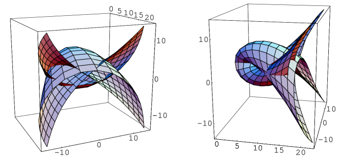
Figure 1: We drawed the same surface from two different points of view. The parameters used in eq. (144) are $a=1,b=0.1,\gamma=\delta=0$

References

- [1] A. Sym, O. Ragnisco, D. Levi and M. Bruschi, Lett. Nuovo Cimento 44, 529 (1991); A.I. Bobenko, ”Surfaces in terms of 2 by 2 matrices, old and new integrable cases”, in Harmonic Maps and Integrable Systems, edited by A.P. Fordy and J.C. Wood, Aspects of Mathematics (Friedr. Vieweg and Sohn, 1994), p. 83.
- [2] O. Ceyhan, A.S. Fokas and M. Gurses, J. Math. Phys. 41, 2251 (2000).
- [3] B.G. Konopelchenko, Stud. Appl. Math. 96, 9 (1996).
- [4] G. Darboux, Leçon sur la théorie générale des surfaces, vol. 4 (Paris, Gauthier-Villars, 1910).
- [5] G. Darboux, Leçon sur les système orthogonaux et les coordenées curvilignes (Paris, Gauthier-Villars, 1910).
- [6] V.E. Zakharov, Duke Math. Journ. 94, 103 (1998); V.E. Zakharov and S.E. Manakov, Dok. Math. 57, 471 (1998).
- [7] R. Dijkgraaf, E. Verlinde and H. Verlinde, Nucl. Phys. B 352, 59 (1991); E. Witten, Nucl. Phys. B 340, 289 (1990).
- [8] L. Martina, O.K. Pashaev and G. Soliani, J. Math. Phys. 38, 1397 (1997).
- [9] S. Deser, R. Jackiw and S. Templeton, Ann. Phys. 180, 372 (1982).
- [10] B.A. Dubrovin, A.T. Fomenko and S.P. Novikov, Modern Differential Geometry (Springer, Berlin, 1984).
- [11] E. Witten, Commun. Math. Phys. 121, 351 (1989).
- [12] The Quantum Hall Effect, edited by S. Girvin and R. Prange (Springer, New York, 1990).
- [13] L. Martina, O.K. Pashaev and G. Soliani, Phys. Rev. D 58, 084025 (1998).
- [14] G. Dunne, Self-dual Chern-Simons theories (Springer, Berlin, 1995).
- [15] L. Martina, O.K. Pashaev and G. Soliani, Mod. Phys. Lett. A 8, 34 (1993).
- [16] V.E. Zakharov and A.B. Shabat, Funct. Anal. Appl. 13, 166 (1979); B.G. Konopelchenko, Introduction to Muldimensional Integrable Equations (Plenum, New York, 1992).
- [17] V.D. Lipovski and A.V. Shirokov, Funct. Anal. and Appl. 23, 225 (1990).
- [18] R.A. Leo, L. Martina and G. Soliani, J. Math. Phys. 33, 1515 (1992).
- [19] T. Eguchi, P.B. Gilkey and A.J. Hanson, Phys. Rep. 66, 213 (1980).
- [20] Y. Ishimori, Prog. Theor. Phys. 72, 33 (1984).
- [21] R. Myrzakulov, S. Vijayalakshmi, G.N. Nugmanova and M. Lakshmanan, Phys. Lett. A 233, 391 (1997).
- [22] R. Myrzakulov, S. Vijayalakshmi, R.N. Syzdykova and M. Lakshmanan, J. Math. Phys. 39, 2122 (1998).
- [23] M. Lakshmanan, R. Myrzakulov, S. Vijayalakshmi and A.K. Danlybaeva , J. Math. Phys. 39. 3765 (1998).
- [24] R. Myrzakulov, G.N. Nugmanova and R.N. Syzdykova, J. Phys. A: Math. Gen. 31, 9535 (1998).
- [25] R. Myrzakulov, A.K. Danlybaeva and G.N. Nugmanova, Theor. Math. Phys. 118, 347 (1999).
- [26] R. Myrzakulov, M. Daniel and R. Amuda, Physica A 234, 715 (1997).
- [27] V.E. Zakharov, in: Solitons, editors R. K. Bullough and P.J. Caudrey (Springer, Berlin 1980).
- [28] Y.C. Ma, Stud. Appl. Math. 59, 201 (1978).
- [29] N. Yajima and M. Oikawa, Prog. Theor. Phys. 56, 1719 (1976).
- [30] I.A. Taimanov, Siberian Math. Journal 40, 1146 (1999).