Probing structures in channel flow through SO(3) and SO(2) decomposition

Abstract

SO(3) and SO(2) decompositions of numerical channel flow turbulence are performed. The decompositions are used to probe, characterize, and quantify anisotropic structures in the flow. Close to the wall the anisotropic modes are dominant and reveal the flow structures. The SO(3) decomposition does not converge for large scales as expected. However, in the shear buffer layer it also does not converge for small scales, reflecting the lack of small scales isotropization in that part of the channel flow.

1 Introduction

Kolmogorov theory of fully developed turbulence has defined the main stream for almost all theoretical and applied turbulence investigations since it appeared in the 1941 (Kolmogorov (1941))
Kolmogorov made two important statements (i) there exists a tendency of any turbulent flow towards isotropization and homogenization of small scales fluctuations, (ii) there exists an inertial range of scales where the ’almost’ isotropic and homogeneous turbulent fluctuations are characterized by a power law spectrum with a universal $-5/3$ slope. Both statements are connected and only partially correct.
First, it is well established experimentally and numerically, Frisch (1995), that already in the ideal isotropic and homogeneous high-Reynolds numbers limit turbulent fluctuations cannot be characterized by only one single set of spectrum exponent, i.e. velocity fluctuations are strongly intermittent. Intermittency is the way to summarize the fact that the probability density of velocity increments, $\delta_{R}u=\left({\mbox{\mbox{\boldmath$u$}}}(\mbox{\mbox{\boldmath$x$}}+{\mbox{\mbox{\boldmath$R$}}})-{\mbox{\mbox{\boldmath$u$}}}(\mbox{\mbox{\boldmath$x$}})\right)\cdot\mbox{\mbox{\boldmath$\hat{R}$}}$, over a distance $R$ cannot be rescaled by using only one single scaling exponents for all $R$, see for example Frisch (1995). Second, in almost all relevant applied situation one is interested in those ranges of scale where turbulence statistics is neither homogeneous nor isotropic.
In the following, as an example, we will discuss in detail the important case of channel flows. Recent experimental, Garg & Warhaft (1998), and numerical investigations, Pumir (1996); Pumir & Shraiman (1995), have shown that the tendency towards the isotropization of small scale statistics of shear-flows is much slower than any dimensional prediction even at very large Reynolds numbers; in contrast to what is predicted by the Kolmogorov 1941 theory, some observables like the skewness of velocity gradients, exhibit persistence of anisotropies. The two above issues are connected. One cannot focus on the issue of intermittency in high-Reynolds number homogeneous and isotropic statistics without first having a systematic control on the possible slowly decaying anisotropic effects always present in all numerical or experimental investigations. Similarly, the understanding of complex non-homogeneous and anisotropic flows cannot avoid the problem of intermittent isotropic and anisotropic fluctuations.

Despite the many systematic theoretical attempts to attack intermittency in isotropic and homogeneous turbulence, the problem is mainly unsolved except for a class of toy-cases considering the passive advection by Gaussian and white in time velocity fields of scalar, Gawedzki & Kupiainen (1995); Chertkov et al. (1995), or vector quantities, Vergassola (1996); Lanotte & Mazzino (1999); Arad et al. (2000). Nevertheless, a lot of phenomenological and analytical progresses have been done by applying standard statistical closure techniques, Kraichnan (1972); Lesieur (1987); L’vov et al. (1997), or more recent phenomenological tools borrowed from dynamical system theory like the fractal and multi-fractals description of the energy transfer and of the energy dissipation rate, Benzi, Paladin, Parisi & Vulpiani (1984); Parisi & Frisch (1983); Frisch (1995); Bohr, Jensen, Paladin & Vulpiani (1998); Benzi, Biferale & Toschi (1998); Grossmann, Lohse & Reeh (2000).
Strangely enough, only very recently, Grossmann et al. (1998); Arad et al. (1998, 1999a, 1999b), similar statistical attempts have been transposed to the understanding of ’non-ideal’ turbulence, i.e., turbulence in all those situations when anisotropy and non-homogeneities play an important role in the turbulent production and dissipation. This paper is meant to partially fill the gap between the quantitative systematic methodology used in ’ideal’ homogeneous and isotropic turbulence and the qualitative, ad-hoc, description in terms of ’structures’ used in the ’non-ideal’ wall bounded flows. We show how the decomposition of statistically stable observable, like moments of velocity increments, in terms of the irreducible representations of the group of rotations in three dimensions, SO(3), and two dimensions, SO(2), allows a quantitative systematic characterization of the isotropic and anisotropic fluctuations. Moreover, a connection between the projections on different eigenvectors of the rotational groups and structures like ’hairpins’ and ’streaks’ is possible.
Structures called ’streaks’ have been thought to be the main signatures of wall bounded flows in the viscous sub-layer since the pioneering works of Kline et al. (1967) who observed the existence of extremely well organized motions made of region of low and high speed fluid, elongated downstream and alternating in the span-wise direction. Later, in Kim et al. (1971), ’streaks’ were reported to be the dynamical responsible of turbulent production in the viscous sub-layer. Similarly, ’hairpins’ have been the main persistent structures observed experimentally, Head & Bandyopanhyay (1981); Wallace (1982), and numerically, Moin & Kim (1985); Kim & Moin (1986), outside the viscous layer, in the turbulent boundary layer. By mean of a conditional sampling, Kim & Moin (1986) were able to show that these ’hairpin’ shaped structures are associated with high Reynolds-shear stress and give a significant contribution to turbulent production in the logarithmic layer.
More recently, Toschi, Amati, Succi, Benzi & Piva (1999); Benzi, Amati, Casciola, Toschi & Piva (1999), started a first systematic investigation of the intermittent properties of velocity increments parallel to the wall as a function of the distance from the wall in a channel flow simulation. In this case a clear transition between the bulk physics and the wall physics was recognized in terms of two different set of intermittent exponents characterizing velocity fluctuations at the center and close to the channel walls. Still a firm quantitative understanding of how much these intermittent quantifiers can be connected to the presence of persistent structures is lacking. For instance, in Benzi et al. (1999) the different behavior of velocity fluctuations in the buffer layer was explained as a breaking of the Kolmogorov refined hypothesis linking energy dissipation to inertial velocity fluctuations, i.e. an effect due to the different production and dissipation mechanism caused by the presence of strong shear effects close to the walls. Clearly, such a kind of issue can only be addressed by using systematic tools which are able to quantify the degree of anisotropy and coherency at difference scales and at different spatial locations in the flow.
In this paper we propose to use the exact decompositions of the correlation functions in terms of the irreducible representations of the rotational group SO(3) (in the bulk of the flow) and in terms of the irreducible representation of the rotational group in two dimensions, SO(2), (close to the walls) in order to quantify in a systematic way the relative and absolute degree of anisotropy of velocity fluctuations. Furthermore, we show how a careful analysis of the data allows also for a connection between some coefficients of the decompositions and the more common ’structures’ observed by simple flow visualization. We show how the SO(3) decomposition, being connected to the exact invariance under rotations of the inertial and diffusive terms of the Navier-Stokes equations, is able, where applicable, to exactly disentangle universal scaling properties of the isotropic sectors from the more complex behavior in the anisotropic sectors. We also show how the SO(2) decompositions in planes parallel to the walls, is a useful analyzing tool in order to quantify the relative change of planar anisotropy by approaching the boundaries.

The paper is organized as follows: In section 2 we review the main theoretical consideration about the importance of the SO(3) decomposition in the Navier-Stokes eqs. In section 3 we present a systematic analysis of the SO(3) decomposition in a numerical channel flow data base. We discuss the results with particular emphasis on the universality issue, i.e. independence from the large scale effects, and on how one can use such a decomposition to quantify the relative importance of structures like ’hairpin’ in the bulk of the flow. In section 4 we review the main findings which pushed us to apply the SO(2) decompositions in planes well inside the buffer layer, i.e. where the SO(3) decomposition cannot be applied due to the presence of the rigid walls, and we show how the SO(2) analysis allows us to clearly distinguish the existence of ’streaks’ like structures in a statistical sense. Section 5 is left to comments and conclusions.

2 SO(3) decomposition

SO(3) – rotational invariance – is one of the basic symmetries of the Navier-Stokes equations. However, it is broken by the boundary conditions or by the driving force of the flow, both of which introduce anisotropy and also inhomogeneities. For the sake of completeness let us start, as an example, with the the SO(3) decomposition of the 2nd order most general velocity tensor depending only on one spatial increment $R$:

$$C_{\alpha\beta}({\mbox{\boldmath$x$}},{\mbox{\boldmath$R$}})=\left<(u_{\alpha}({\mbox{\boldmath$x$}}+{\mbox{\boldmath$R$}})-u_{\alpha}({\mbox{\boldmath$x$}})(u_{\beta}({\mbox{\boldmath$x$}}+{\mbox{\boldmath$R$}})-u_{\beta}({\mbox{\boldmath$x$}})\right>$$ (1)

It is easy to realize, Arad et al. (1999b), that this observable can be decomposed in terms of the irreducible representations of the three dimensional rotational group which form a complete basis in the space of smooth second order tensors depending on one vector $R$:

$$C_{\alpha\beta}({\mbox{\boldmath$x$}},{\mbox{\boldmath$R$}})=\sum_{qjm}a_{q,jm}({\mbox{\boldmath$x$}},R)B_{\alpha\beta}^{q,jm}({\mbox{\boldmath$\hat{R}$}}),$$ (2)

The notation in (2) is borrowed from the quantum mechanical analogue, i.e. $j=0,1,....$ labels the eigenvalues of the modulus of the total angular momentum, ${\bf L^{2}}$; $m=-j,..,+j$ labels the eigenvalues of the projection of the total angular momentum on one direction, say $\hat{y}$; $q$ labels the different irreducible representations with a given $j$; and $B_{\alpha\beta}^{q,jm}({\mbox{\boldmath$\hat{R}$}})$ are the eigenfunction of the rotational group in the space of second order smooth tensors. For example for the fully isotropic sector, $j=0$, we have only $m=0$ and a simple calculation shows that there are only two independent irreducible representations in the isotropic sectors, i.e. the well known result, Monin & Yaglom (1975), that we need only two independent eigenfunction in order to describe any second order isotropic tensor. These two eigenfunction can be taken to be:

$$B_{\alpha\beta}^{1,00}({\mbox{\boldmath$\hat{R}$}})=\delta_{\alpha,\beta};\;\;\;\;B_{\alpha\beta}^{2,00}({\mbox{\boldmath$\hat{R}$}})={\bf\hat{R}}_{\alpha}{\bf\hat{R}}_{\beta}$$

and therefore the decomposition (2) in the isotropic sector assumes the familiar form:

$$C_{\alpha\beta}({\mbox{\boldmath$x$}},{\mbox{\boldmath$R$}})=a_{1,00}({\mbox{\boldmath$x$}},R)\delta_{\alpha,\beta}+a_{2,00}({\mbox{\boldmath$x$}},R){\mbox{\boldmath$\hat{R}$}}_{\alpha}{\mbox{\boldmath$\hat{R}$}}_{\beta}$$ (3)

In appendix A we list the complete set of $B_{\alpha\beta}^{q,jm}$ for the case of second order tensors. For higher tensor ranks we refer to Arad et al. (1999b). The main physical information is of course hidden in the dependence of the coefficients $a_{q,jm}({\mbox{\boldmath$x$}},R)$ on the spatial location, $x$, and on the analyzed scale, $R$. We aim at using the decomposition (2) as a filter able to exactly disentangle different anisotropic effects as a function of the spatial location and of the analyzed scale. In previous studies, the main interest was focused on the theoretical issue of the existence of scaling behavior for the coefficients $a_{q,jm}({\mbox{\boldmath$x$}},R)$ and on its possible dynamical explanation in terms of the ’foliation’ of the Navier-Stokes eqs in different $j$ sectors, Arad et al. (1998, 1999a, 1999b). The typical questions addressed were whether coefficients belonging to different $j$ sectors have different scaling behavior (if any) and, in the case, which kind of dimensional estimate for scaling exponents in the anisotropic sectors one could propose. As for the issues of scaling behavior, due to the limitation of small Reynolds numbers in the numerical case (Arad et al. (1999a)), and to the limited amount of information available on the tensorial structure of the velocity field in the experimental case (Arad et al. (1998); Kurien et al. (2000)) only partial answers have been found. Among them, the most important is the strong universality shown by the isotropic sector as a function of the local degree of non-homogeneity (and anisotropy), i.e. the strong universality showed by the scaling properties of the coefficients $a_{q,00}({\mbox{\boldmath$x$}},R)$ as a function of $x$ in non-homogeneous turbulence (Arad et al. (1999a)). On the other hand, in this paper we would like to also propagate the SO(3) decomposition as an appropriate tool to analyze, characterize, and quantify the non-universal large scale geometric properties of the turbulent flow.
As an example we take numerical channel flow (Amati, Succi & Piva (1997); Toschi, Amati, Succi, Benzi & Piva (1999)) obtained by a lattice Boltzmann code running on a massively parallel machine. The spatial resolution of the simulation is $256\times 128\times 128$ grid points. Periodic boundary conditions were imposed along the stream-wise (x) and span-wise (z) directions, whereas no slip boundary conditions were applied at the top and at the bottom planes (y-direction). The Reynolds number at the center of the channel is about 3000. In our case of channel flow we assume that, due to the homogeneity in planes parallel to the walls, there is only a dependence on the height $y$ of all statistical observable. The coefficients $a_{q,jm}({\mbox{\boldmath$x$}},R)$ carry two types of information: (i) Their scaling behavior $a_{q,jm}({\mbox{\boldmath$x$}},R)\propto R^{\zeta^{(2)}_{q,jm}}$ which at least for small scales and large $Re$ is hoped to be universal, i.e., position and flow independent and (ii) their absolute or relative magnitudes which clearly are non-universal, i.e., position $x$ and flow type dependent. These ratios characterize what kind of structures the flow contains. These are time and ensemble averaged quantities, obeying the underlying Navier-Stokes SO(3) symmetry, and we consider them to be a more systematic tool for structures characterization than snapshots of vortex sheets, worms, swirls or contour plots of either the velocity or the vorticity fields.

When analyzing higher order structure tensors $C_{\alpha\beta\dots\gamma}({\mbox{\boldmath$x$}},{\mbox{\boldmath$R$}})$ the decomposition of type (2) becomes cumbersome soon. Moreover, in most experiments the full tensorial information is not available anyhow. Therefore, one has to restrict oneself to an abbreviated form of the SO(3) decomposition of the velocity structure tensor, namely, the SO(3) decomposition of the longitudinal structure function. In this case, being the undecomposed observable a scalar under rotations, there exists only one irreducible representation for any $j$ sector, i.e. the usual spherical harmonics basis set $Y_{jm}({\mbox{\boldmath$\hat{R}$}})$. We decompose the longitudinal structure function

$$S_{L}^{(p)}({\mbox{\boldmath$x$}},{\mbox{\boldmath$R$}})=\left\langle\left(\left({\mbox{\boldmath$u$}}\left({\mbox{\boldmath$x$}}+{\mbox{\boldmath$R$}}\right)-{\mbox{\boldmath$u$}}\left({\mbox{\boldmath$x$}}-{\mbox{\boldmath$R$}}\right)\right)\cdot{\mbox{\boldmath$\hat{R}$}}\right)^{p}\right\rangle$$ (4)

as follows:

$$S_{L}^{(p)}({\mbox{\boldmath$x$}},{\mbox{\boldmath$R$}})=\sum_{jm}{S_{jm}^{(p)}({\mbox{\boldmath$x$}},R)Y^{jm}({\mbox{\boldmath$\hat{R}$}})}.$$ (5)

We expect that when scaling behavior sets in (presumably at high enough Re) we should find:

$$S^{(p)}_{jm}({\mbox{\boldmath$x$}},R)\sim a_{jm}({\mbox{\boldmath$x$}})R^{\zeta_{jm}^{(p)}}\ .$$ (6)

Again, the $a_{jm}^{(p)}({\mbox{\boldmath$x$}},R)$ carry both the scaling information $a_{jm}^{(p)}({\mbox{\boldmath$x$}},R)\propto R^{\zeta_{jm}^{(p)}}$ and their non-universal amplitudes.
A practical problem with the decomposition (5) of (4) is that for $x$ close to the boundaries the scale $R$ is restricted to lengths smaller than the distance from the wall. More generally, $R$ cannot exceed a typical distance over which non homogeneities are overwhelming. Therefore we will also perform a decomposition of (4) which obeys the weaker SO(2) symmetry, i.e. rotational invariance in a plane for fixed distance $y$ from the wall,

$$D_{L}^{(p)}(y,{\mbox{\boldmath$R$}})=\sum_{m}d_{m}^{(p)}(y,R)\exp{(im\phi)}.$$ (7)

The orientation dependence in a plane reduces to the dependence on an angle $\phi$. Again, the $d_{m}^{(p)}(y,R)$ carry both scaling and amplitude information.

Let us notice at this point, that the SO(3) decomposition has its roots on the intimate structure of the Navier-Stokes eqs, i.e on the invariance under rotations of the inertial and dissipative terms and on the relative foliations on different sectors of the rotational group of the equation of motion of any correlation function Arad et al. (1999b). On the other hand, do not exist closed equations for two-dimensional observable and therefore the SO(2) decomposition can only be seen as a powerful tool to exactly decompose any observable in a fixed plane as a function of isotropic and anisotropic structures in the plane itself. Clearly, such a kind of decomposition can teach us a lot in those regions, like at the border between the viscous and turbulent boundary layers, where strongly anisotropic but planar structures named ’streaks’ are supposed to carry the most important dynamical information of the flow.

3 SO(3) analysis of a turbulent channel flow field

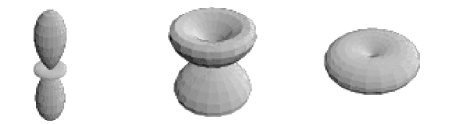
Figure 4: Graphical representation of spherical harmonics (from left to right) $\left|Y^{2,0}(\theta,\phi)\right|$, $\left|Y^{2,1}(\theta,\phi)\right|$ and $\left|Y^{2,2}(\theta,\phi)\right|$.

In previous studies most of the attention was paid on the isotropic sector of the structure function decomposition (5), i.e. on the behavior of $S_{00}^{(p)}({\mbox{\boldmath$x$}},R)$ as a function of the center of the decomposition, $x$, and of the scale $R$. In Arad et al. (1999a) it was showed that the isotropic projection enjoys much better scaling properties than the undecomposed structure function and that these properties are robust with respect to the changing of the local degree of anisotropy, i.e. with respect to the center of the decomposition, $x$. These findings support the idea of universality of the isotropic scaling exponents.Very little was possible to say about scaling of the anisotropic sectors because of lack of spatial resolution; the only qualitative statement was that the scaling exponent of the $j=2$ sector was roughly $4/3$, as predicted by the dimensional argument given by Lumley (1967) or by Grossmann et al. (1994).
Here we want to concentrate also on the more applied question of how much the different projections, independently on their possible scaling properties, can teach us about the preferred geometrical structures present in the flow at changing the analyzing position in the channel.
In figs. 2 and 3 we present the three different contributions we have in the $j=2$ non-isotropic sector extracted at the center of the channel ($y^{+}=160$) and at one quarter ($y^{+}=80$) respectively.
The relative size of the $S_{2m}^{(2)}(y^{+},R^{+})$ for different $m$ and fixed $y^{+}$ characterize the geometry of the anisotropic structures on the corresponding scale $R$. E.g., for $y^{+}=80$ the $(j=2,m=1)$ mode is very pronounced on smaller scales, see fig. 3. We associate this with the hairpin vortices and other structures which diagonally detach from the wall and which are projected out by $Y_{21}$. For a visualization of the $Y_{2m}$ see figure 4. In the center the $(j=2,m=1)$ mode is two orders of magnitude less pronounced than at $y^{+}=80$. Our interpretation is that the diagonal structures from above and below have equal and opposite contributions.
The most pronounced structures in the center are those parallel to the flow direction, i.e., $(j=2,m=2)$, see figure 2.
Also at $y^{+}=80$ the structures parallel to the flow direction (mode $(j=2,m=2)$) are rather pronounced. At scales beyond $R^{+}\approx 100$ they overwhelm the diagonal contributions (mode $(j=2,m=1)$). Therefore one is tempted to interpret $R^{+}\approx 100$ as the maximal size (in average) of the hairpin vortices.
We re-did this type of analysis also for the $S_{2m}^{(4)}(y^{+},R^{+})$ with very similar results.

3.1 Higher order moments and the lack of isotropy at small scales

The first question one may want to ask about the decomposition (5) is whether it converges with increasing $j$. We want to check this for an $R$ in (stream-wise) flow direction, i.e., ${\mbox{\boldmath$\hat{R}$}}=(\theta,\phi)=(\pi/2,0)$. As we can see from fig. 5, at small scales and in the channel center, where anisotropic contributions are small, the convergence is rather good. But away from the center ($y^{+}=62$) and in particular for large scales quality of the convergence become poor, see fig. 6. Note that in any case the convergence is not monotonous as a function of the scale. This is a systematic quantitative way to understand the rate of isotropization toward small scales exhibited by this particular flow as a function of the distance from the wall.

Another, even more informative way to quantify the rate of isotropization is to plot the ratio of each single amplitude $S_{jm}^{(2)}({\mbox{\boldmath$x$}},R)$ to the total structure function $S_{L}^{(2)}({\mbox{\boldmath$x$}},{\mbox{\boldmath$R$}})$ with $R$ in the direction of the mean flow. In figs. 7 and 8 one can find the above quantities at the center of the channel $y^{+}=160$ and in the buffer layer $y^{+}=62$, respectively. What is very interesting to notice is that at large scales there are contributions from all resolved $j$ sectors indicating as expected a lack of convergence of the decomposition at those scales and that in the buffer layer the relative ratio of the anisotropic sectors is much higher than what is seen in the center. Moreover, even more interesting, in the buffer layer, where due to the presence of a high shear one can imagine a statistically stable signature of anisotropic physics there appears a clear grouping of different sectors labeled by different $j$ indexes. Fig. 8 shows that projections with the same $j$ but different $m$ indexes have a qualitative similar behavior. Of course, these kind of comparison depends on the direction of the undecomposed structure functions (here taken parallel to the walls).
Another possible test of the relative weights of anisotropies, free of the previous arbitrariness, is to plot the ratio between the isotropic projection $S_{00}^{(p)}({\mbox{\boldmath$x$}},R)$ and the other anisotropic projections for $j>0$. Such a test is done in terms of quantities depending only on the separation magnitude $|R|$, and therefore measures the relative importance of anisotropies independently of the orientation. In Fig 9 we show, for example, the ratio between the sector $(j,m)=(4,4)$ and the isotropic sector $(j,m)=(0,0)$ at changing the analyzed height in the channel and for all $R^{+}$. As it is possible to see, as expected, by approaching the wall (decreasing $y^{+}$) the ratio becomes larger and larger, showing clearly the importance of high $j$ fluctuations in the sheared buffer layer.
All the previous trends have also been found, amplified, by analyzing higher moments. For example, in figs. 10 and 11 we re-plot the same of figs. 7 and 8 but for the fourth order structure functions. The fact that the previous trends are much more enhanced for higher order moments is a clear indication that anisotropy fluctuations are important but ’rare’, i.e. are connected to persistent intense fluctuations in a sea of isotropic turbulence.

4 SO(2) analysis of a turbulent channel flow

As extensively discussed in the previous sections, the SO(3) decomposition turned out to be extremely useful from both its theoretical background connected to the symmetry of the NS eqs and its ability to highlights statistical information as a function of their geometrical structures. On the other hand, the SO(3) decomposition suffers from some drawbacks when one wants to analyze the statistical turbulent behavior close to the fluid boundaries. This is due to the obvious fact that in order to perform the decomposition one needs to perform integrals over a given sphere, and therefore close to the boundaries the limitation of the sphere radius does not allow to extract any information but for a very limited (almost fully dissipative) range of scales.
To overcome this problem we propose to use a decomposition in eigenfunction of the group of rotations in two dimensions, SO(2). The rational behind this idea is that the Navier Stokes equations obviously obey the $SO(2)$ symmetry and for the channel flow also the geometry obeys this symmetry, once the rotation axis is chosen in the $y$ direction. However, the mean flow breaks the $SO(2)$ symmetry as it breaks the $SO(3)$ symmetry. Nevertheless we will gain a tool being able to exactly decompose any two-dimensional observable in terms of fluctuations with a given property under two-dimensional rotations. In the region very close to the walls where very elongated ’streak’ structures have been observed, the SO(2) analysis may help in understanding the relative importance of isotropic (in the plane) and anisotropic (in the plane) fluctuations.
Another very important issue we want to address by using the SO(2) decomposition is connected to the recent findings by Toschi et al. (1999) of a different intermittent behavior close to the walls ($y^{+}\sim 35$) shown by longitudinal structure functions in the stream-wise direction. These results were also connected to the breaking of the Refined Kolmogorov Similarity Hypothesis (RKSH) in the buffer layer, Benzi et al. (1999). Here, we show that by means of the SO(2) decomposition we are able to highlight the importance of the streak like structures in determining this higher intermittent behavior.
In this section we are interested only in observable in planes parallel to the walls and therefore the SO(2) decomposition of, say, the longitudinal structure function is defined as

$$D_{L}^{(p)}\left(y,{\mbox{\boldmath$R$}}\right)=\sum_{m}d_{m}^{(p)}\left(y,R\right)\exp{(\left(im\phi\right))},$$ (8)

where $R$ is a two-dimensional vector lying in a plane at fixed $y$, and $D_{L}^{(p)}(y,{\mbox{\boldmath$R$}})$ is the longitudinal structure function in the direction $R$. Due to the symmetry of the structure function we expect that only even $m$s will contribute to the sum in (8)
In Fig. 12 and Fig. 13 we show the rate of convergence of the reconstructed structure function of order 2 as function of the maximum $M$ contributing to the right hand side (RHS) of (8) and at two different distances from the wall, at the center (fig. 12) and in the buffer layer (fig. 13). As it is clear, again we find a quite good convergence in the center. In the buffer layer, especially large scales are still far from being reconstructed even reaching $M=8$. This is a clear tendency of formation of very large and intense structures in the strongly anisotropic buffer. These trends are even more pronounced for the fourth order moment as shown in Figs. 14 and 15.
In Fig. 16 we show the absolute weight of different $m$-contributions for the second order structure function again in the center. It is interesting to notice that there is a clear monotonic organization of different contributions as a function of their isotropic/anisotropic properties, i.e. higher $m$s are less intense than lower $m$s systematically way at all scales.
On the other hand, in the buffer layer, Fig. 17, there is a crossing of the $m=2$ contribution and of the $m=4$ contribution at scales of the order of $R^{+}\sim 90$. We interpret this crossing as the evidence of the formation of structures with typical size $R^{+}\sim 90$ and with a preferred orientation given by the $m=2$ eigenfunction. The $m=2$ eigenfunction weights preferentially structures with a positive correlation in the stream-wise direction and negative correlated in the span-wise direction, i.e. exactly ’streak’ like structures as those observed also in our numerical simulation by performing simple contour plots (see Fig. 20). As it is always the case, the above observed trends are even more intense for $p=4,6..$. For $p=6$ it even happens (not shown) that the dominant contribution at large scales is given by the $m=2$ sector, proving, once more, the extreme departure from isotropy (in the plane) close to the walls.
In order to quantify the departure from isotropy in each planes at changing the distance from the wall we plot the ratios between the projections on the $m=2$ sector and the isotropic sector (Fig. 18) at varying the distance from the wall and for some $R^{+}$ values. Fig. 19 shows the same but for $m=4$. It is interesting to notice, how there is a sharp transition for $y^{+}\sim 40$ from an almost isotropic statistics ($y^{+}>40$) and a strongly anisotropic statistics ($y^{+}<40$), again the clear signature of the beginning of a “structured” buffer for $(y^{+}<40)$ shows up.

4.1 Review of near wall physics

Let us now switch to the more statistically minded question connected to the existence of different intermittent properties close to the walls as previously reported in Toschi et al. (1999). This issue is connected to the general question whether in strong shear regions for a range of scales larger than the typical shear length, $L_{{\cal S}}=\left(\varepsilon/{\cal S}^{3}\right)^{1/2}$, one may have a different statistic transfer of energy than what expected at scales smaller than the typical shear length. Different statistical energy transfer properties would have as a consequence also different intermittent properties of the velocity structure functions and, probably, the breaking of the RKSH if the shear lengths is small enough to be comparable with the dissipative length. Only in very high sheared region one can hope to have a very small $L_{S}$ and therefore a sufficient range of scales with $R>L_{S}$ where scaling laws can be investigated. Indeed in many different sheared flows, Onorato et al. (2000); Benzi et al. (1996b); Gaudin et al. (1998), it has been found that in strongly sheared region intermittency increase and display universality (i.e. same exponents were measured in very different set-up). In Toschi et al. (2000) it was given a simple theoretical explanation of how intermittency should change in presence of strong shear. Considering the usual decomposition of the velocity field in its average and fluctuating part, ${\mbox{\mbox{\boldmath$v$}}}(\mbox{\mbox{\boldmath$x$}};t)={\overline{{\mbox{\mbox{\boldmath$v$}}}}}(\mbox{\mbox{\boldmath$x$}})+{\mbox{\mbox{\boldmath$v$}}}^{\prime}(\mbox{\mbox{\boldmath$x$}};t)$, we get (from the Navier-Stokes equations) the usual Reynolds decomposition

$$D_{t}v^{\prime}_{i}+{\cal S}_{ij}(\mbox{\mbox{\boldmath$x$}})v^{\prime}_{j}+v_{j}^{\prime}\partial_{j}v^{\prime}_{i}-{\overline{v_{j}^{\prime}\partial_{j}v^{\prime}_{i}}}=-\partial_{i}p^{\prime}+\nu\Delta v^{\prime}_{i}$$ (9)

with $D_{t}=\left(\partial_{t}+{\overline{v}}_{j}\partial_{j}\right)$. The shear is defined as ${\cal S}_{ij}\left(\mbox{\mbox{\boldmath$x$}}\right)=\partial_{j}{\overline{v}_{i}\left(\mbox{\mbox{\boldmath$x$}}\right)}$ and depends on the mean flow geometry.

In equation 9 the second and third terms of left hand side (LHS) will be of the same order at a scale $L_{{\cal S}}\sim\left(\epsilon/S^{3}\right)^{1/2}$ (shear length scale). For scale smaller than $L_{{\cal S}}$ it is the third term in eqn. 9 that will balance the energy dissipation, and hence the usual Refined Kolmogorov Similarity Hypothesis will hold: $S_{p}(r)\sim\left\langle\varepsilon(r)^{p/3}\right\rangle\cdot r^{p/3}$. For scales larger than $L_{{\cal S}}$ it will be the second term in eqn. 9 that will balance the energy dissipation and hence: $S_{p}(r)\sim\left\langle\varepsilon(r)^{p/2}\right\rangle$. The validity of this second relation i n region of high shear values was already established by Benzi et al. (1999).
We want now to see how much one can say about this new ’intermittent’ behavior close to the channel walls. In order to extract any quantitative information on scaling exponents in numerical simulation one needs to use the ESS technique, Benzi et al. (1993, 1996a); Grossmann et al. (1997). ESS is based on the experimental and numerical observation that structure functions even at moderate Reynolds numbers show scaling in a generalized sense, i.e. by studying the relative scaling of one structure functions, say the second order structure function, versus any other. In particular, we want to verify and exploit that the following scaling holds:

$$D_{L}^{(p)}(y,{\mbox{\boldmath$R$}})\sim\left(D_{L}^{(2)}(y,{\mbox{\boldmath$R$}})\right)^{\zeta_{y}^{(p)}/\zeta_{y}^{(2)}}$$ (10)

where we have again limited ourself to the analysis of structure functions in the plane. In (10) we have explicitly taken into account the possibility that the scaling exponents depend on the distance from the walls. In particular, Toschi et al. (1999) showed, by analyzing the same data set, that there exist two distinguished set of exponents. One governing the scaling in the range of scales smaller than $L_{S}$ (i.e. close to the center of the channel, in our case) which is given in terms of the usual isotropic and homogeneous set of exponents. The second governing the scaling in the sheared range of scales $R>L_{S}$ (i.e. close to the walls in our channel simulation) which is given in terms of a much more intermittent set of exponents.
In Fig. 21 we show the ESS local slopes of the undecomposed structure function in the stream-wise direction in the center of the channel and the ESS local slope of the projection on the $m=0$ sector always at the center of the channel for the moments $p=2$ versus $p=4$. As it is evident, already the fully isotropic component (in the plane) is able to well reproduce the undecomposed observable and are both in good agreement with the isotropic and homogeneous scaling. Of course, the previous finding confirms the simple statement that at the center of the channel the shear length is formally infinite and therefore the whole range of scales available is weakly affected by any shear effect. On the other hand in Fig. 22 we show the same quantities of Fig. 21 but in a plane well inside the buffer layer ($y^{+}=37$). As it is possible to see now the $m=0$ component does not reproduce the undecomposed observable, confirming the evident fact that here we are strongly anisotropic. Nevertheless, it is enough to add the $m=2$ sector, i.e. to reconstruct up to $M=2$ in the RHS of (8) to have a very good agreement with the more intermittent undecomposed structure functions local slope. This is a good quantitative evidence that as far as the new scaling properties are concerned the main effects is brought by these $m=2$ ’streak’ like structures in the buffer layer.
Still we need to understand the physics of these structures, why they are more intermittent, whether it is a coincidence or not that the new set of exponents coincides extremely well with what measured for passive scalar advected by a turbulent flow Chavarria et al. (1995). Nevertheless, we are confident that having a systematic way to analyze any isotropic/anisotropic two-dimensional/three-dimensional turbulent data set may help in further advance of the field.

5 Conclusions

A detailed investigation of anisotropies in channel flows in terms of the SO(3) and SO(2) decomposition of structure functions has been presented. Projections on the eigenfunction of the two symmetry groups can be seen as a systematic expansions of structures as a functions of their scale and in terms of their local degree of anisotropy.
We have used the SO(3) decomposition of structure functions at the center and at one quarter of the channel in order to have a quantitative tool to measure the relative importance of isotropic and anisotropic fluctuations at all scales. Close to the wall, the anisotropic fluctuations show strong effects induced from structure with the typical orientations of hairpin vortices. A partial lack of isotropization is still detected at the smallest resolved scales.
The SO(2) decomposition in planes parallel to the walls allowed us to access also the viscous and buffer regions. In those regions, we have found that the strong enhancement of intermittency can be understood in terms of streak like structures and their signatures in some coefficients of the SO(2) decomposition.
We think that the method presented here is beneficially applicable in all those cases where quantitative comparison and/or studies of anisotropic effects in different flows are needed (channel flows, boundary layers, homogeneous shear etc..)
The application of similar decomposition to small scales observable like vorticity and energy dissipation would certainly be of great interest too.
Having the possibility to control the anisotropic behavior is of great importance to improve LES of strongly anisotropic and inhomogeneous flows.

Acknowledgments: The authors thank I. Arad for I. Procaccia for helpful discussions. The work is part of the research program of the Stichting voor Fundamenteel Onderzoek der Materie (FOM), which is financially supported by the Nederlandse Organisatie voor Wetenschappelijk Onderzoek (NWO). This research was also supported in part by the European Union under contract HPRN-CT-2000-00162 and by the National Science Foundation under Grant No. PHY94-07194 and we thank the Institute of Theoretical Physics in Santa Barbara for its hospitality.

6 Appendix A

In this appendix, we want to explicitly write down the SO(3) decomposition of the most general two-point velocity correlations in anisotropic turbulence. We consider the second order tensor involving velocities at two distinct points ${\bf x_{1}}={\bf x}$ and ${\bf x_{2}}={\bf x+R}$:

$$C^{\alpha\beta}({\mbox{\boldmath$R$}})\equiv\left\langle u^{\alpha}({\mbox{\boldmath$R$}})u^{\beta}({\mbox{\boldmath$R$}}+{\mbox{\boldmath$x$}})\right\rangle\;.$$ (11)

where we have supposed that the statistics is homogeneous (but not isotropic) and therefore the LHS of (11) depends only on ${\bf R}$, the distance between the two points. Then, we can decompose $C^{\alpha\beta}$ according to the irreducible representations of the SO(3) groups. Each irreducible representations will be composed by a set of functions labeled with the usual indices $j=0,1,....$ and $m=-j,...,+j$ corresponding to the total angular momentum and to the projection of the total angular momentum on a arbitrary direction respectively. Moreover, a new ’quantum’ index $q$ which labels different irreducible representations will be necessary. It is easy to realize that there are only $q=1,...,9$ irreducible representations of the SO(3) groups on the space of two-indices tensor depending continuously from a three-dimensional vector, Arad et al. (1999b). In particular, fixed $j$ and $m$, the $9$ basis tensor can be simply constructed starting from the scalar spherical harmonics $Y_{j,m}(\hat{\bf X})$ plus successive application of the two isotropic operators $R_{\alpha}$ and $\partial_{\beta}$ in order to saturate the correct number of tensorial indices. For example, the $9$ linearly independent basis vectors which defines the irreducible representations in our case can be chosen as:

$$B_{1,jm}^{\alpha\beta}({\mbox{\boldmath$\hat{R}$}}) \equiv R^{-j}\delta^{\alpha\beta}\Phi_{jm}({\mbox{\boldmath$R$}})\;,$$

$$B_{2,jm}^{\alpha\beta}({\mbox{\boldmath$\hat{R}$}}) \equiv R^{-j+1}\epsilon^{\alpha\beta\mu}\partial_{\mu}\Phi_{jm}({\mbox{\boldmath$R$}})\;,$$

$$B_{3,jm}^{\alpha\beta}({\mbox{\boldmath$\hat{R}$}}) \equiv R^{-j}[x^{\alpha}\partial^{\beta}-R^{\beta}\partial^{\alpha}]\Phi_{jm}({\mbox{\boldmath$R$}})\;,$$

$$B_{4,jm}^{\alpha\beta}({\mbox{\boldmath$\hat{R}$}}) \equiv R^{-j-1}\epsilon^{\alpha\beta\mu}R_{\mu}\Phi_{jm}({\mbox{\boldmath$R$}})\;,$$

$$B_{5,jm}^{\alpha\beta}({\mbox{\boldmath$\hat{R}$}}) \equiv R^{-j+2}\partial^{\alpha}\partial^{\beta}\Phi_{jm}({\mbox{\boldmath$R$}})\;,$$

$$B_{6,jm}({\mbox{\boldmath$\hat{R}$}}) \equiv R^{-j+1}[\epsilon^{\beta\mu\nu}R_{\mu}\partial_{\nu}\partial^{\alpha}+\epsilon^{\alpha\mu\nu}R_{\mu}\partial_{\nu}\partial^{\beta}]\Phi_{jm}({\mbox{\boldmath$R$}})\;,$$

$$B_{7,jm}^{\alpha\beta}({\mbox{\boldmath$\hat{R}$}}) \equiv R^{-j}(x^{\alpha}\partial^{\beta}+R^{\beta}\partial^{\alpha})\Phi_{jm}({\mbox{\boldmath$R$}})\;,$$

$$B_{8,jm}^{\alpha\beta}({\mbox{\boldmath$\hat{R}$}}) \equiv R^{-j-1}[x^{\alpha}\epsilon^{\beta\mu\nu}R_{\mu}\partial_{\nu}+R^{\beta}\epsilon^{\alpha\mu\nu}R_{\mu}\partial_{\nu}]\Phi_{jm}({\mbox{\boldmath$R$}})\;,$$

$$B_{9,jm}^{\alpha\beta}({\mbox{\boldmath$\hat{R}$}}) \equiv R^{-j-2}x^{\alpha}R^{\beta}\Phi_{jm}({\mbox{\boldmath$R$}})\;.$$

Where for the sake of simplicity we have posed $\Phi_{jm}({\mbox{\boldmath$R$}})\equiv R^{j}\,Y_{jm}({\mbox{\boldmath$\hat{R}$}})$. As a results the most general second order tensor like (11) can be decomposed as:

$$C^{\alpha\beta}({\mbox{\boldmath$R$}})\equiv\sum_{j,m}\sum_{q=1}^{9}c_{q,jm}(R)B^{\alpha\beta}_{q,jm}({\mbox{\boldmath$\hat{R}$}})$$ (12)

where now the physics of the anisotropic statistical fluctuations must be analyzed in terms of the projections $c_{j,m,q}(R)$ in the different sectors.

Figure 1: Coordinate system in channel. Shown are stream-wise ($x$), span-wise ($z$) and wall-normal ($y$) directions.

Figure 2: Log-log plot of $S^{(2)}_{2,2}(y^{+},R^{+})~{}(\ast)$; $S^{(2)}_{2,1}(y^{+},R^{+})~{}(\times)$ and $S^{(2)}_{2,0}(y^{+},R^{+})~{}(+)$ as functions of $R^{+}$ at the center of the channel $y^{+}=160$.

Figure 3: Log-log plot of $S^{(2)}_{2,2}(y^{+},R^{+})~{}(\ast)$; $S^{(2)}_{2,1}(y^{+},R^{+})~{}(\times)$ and $S^{(2)}_{2,0}(y^{+},R^{+})~{}(+)$ as functions of $R^{+}$ at $y^{+}=80$.

Figure 5: Analysis of the convergence of the $SO(3)$ decomposition: $ratio_{J,M}$ represents the ratio between the longitudinal structure function of order $2$ in the stream-wise direction reconstructed up to $(J,M)=(0,0)~{}(+)$; $(J,M)=(2,0)~{}(\times)$; $(J,M)=(2,2)~{}(\ast)$; $(J,M)=(4,0)~{}(\square)$; $(J,M)=(4,2)~{}(\blacksquare)$ and $(J,M)=(4,4)~{}(\circ)$ and the undecomposed structure function, at the center of the channel $y^{+}=160$.

Figure 6: Analysis of the $SO(3)$ decomposition’s convergence: $ratio_{J,M}$ represents the ratio between the longitudinal structure function of order $2$ in the stream-wise direction reconstructed up to $(J,M)=(0,0)~{}(+)$; $(J,M)=(2,0)~{}(\times)$; $(J,M)=(2,2)~{}(\ast)$; $(J,M)=(4,0)~{}(\square)$; $(J,M)=(4,2)~{}(\blacksquare)$ and $(J,M)=(4,4)~{}(\circ)$ and the undecomposed structure function, at the center of the channel $y^{+}=62$

Figure 7: Ratio of each single $(j,m)$ amplitude $S^{(2)}_{j,m}(y^{+},{\mbox{\boldmath$R$}})$ to the total structure function $S^{(2)}_{L}(y^{+},{\mbox{\boldmath$R$}})$ with ${\bf R}$ in the direction of the mean flow and $y^{+}=160$. The $(j,m)$ indexes are: $(0,0)~{}(+)$; $(2,0)~{}(\times)$; $(2,2)~{}(\ast)$; $(4,0)~{}(\square)$; $(4,2)~{}(\blacksquare)$ and $(4,4)~{}(\circ)$.

Figure 8: Ratio of each single $(j,m)$ amplitude $S^{(2)}_{j,m}(y^{+},{\mbox{\boldmath$R$}})$ to the total structure function $S^{(2)}_{L}(y^{+},{\mbox{\boldmath$R$}})$ with ${\bf R}$ in the direction of the mean flow and $y^{+}=62$. The $(j,m)$ indexes are: $(0,0)~{}(+)$; $(2,0)~{}(\times)$; $(2,2)~{}(\ast)$; $(4,0)~{}(\square)$; $(4,2)~{}(\blacksquare)$ and $(4,4)~{}(\circ)$.

Figure 9: Ratios between the sector $(j,m)=(4,4)$ of the decomposition of $S^{(2)}_{L}(y^{+},R^{+})$ and the isotropic sector $(j,m)=(0,0)$ as functions of R, at changing the analyzed height in the channel: $y^{+}=160~{}(+)$; $y^{+}=125~{}(\times)$; $y^{+}=92~{}(\ast)$; $y^{+}=80~{}(\square)$; $y^{+}=62~{}(\blacksquare)$; $y^{+}=48~{}(\circ)$ and $y^{+}=37~{}(\bullet)$.

Figure 10: Ratio of each single $(j,m)$ amplitude $S^{(4)}_{j,m}(y^{+},{\mbox{\boldmath$R$}})$ to the total structure function $S^{(4)}_{L}(y^{+},{\mbox{\boldmath$R$}})$ with ${\bf R}$ in the direction of the mean flow and $y^{+}=160$. The $(j,m)$ indexes are: $(0,0)~{}(+)$; $(2,0)~{}(\times)$; $(2,2)~{}(\ast)$; $(4,0)~{}(\square)$; $(4,2)~{}(\blacksquare)$ and $(4,4)~{}(\circ)$.

Figure 11: Ratio of each single $(j,m)$ amplitude $S^{(4)}_{j,m}(y^{+},{\mbox{\boldmath$R$}})$ to the total structure function $S^{(4)}_{L}(y^{+},{\mbox{\boldmath$R$}})$ with ${\bf R}$ in the direction of the mean flow and $y^{+}=62$. The $(j,m)$ indexes are: $(0,0)~{}(+)$; $(2,0)~{}(\times)$; $(2,2)~{}(\ast)$; $(4,0)~{}(\square)$; $(4,2)~{}(\blacksquare)$ and $(4,4)~{}(\circ)$.

Figure 12: Analysis of the convergence of the $SO(2)$ decomposition: $ratio_{M}$ represents the ratio between the longitudinal structure function of order $2$ in the stream-wise direction reconstructed up to $M=0~{}(+)$; $M=2~{}(\times)$; $M=4~{}(\ast)$; $M=6~{}(\square)$ and $M=8~{}(\blacksquare)$ and the undecomposed structure function, at the center of the channel $y^{+}=160$

Figure 13: Analysis of the convergence of the $SO(2)$ decomposition: $ratio_{M}$ represents the ratio between the longitudinal structure function of order $2$ in the stream-wise direction reconstructed up to $M=0~{}(+)$; $M=2~{}(\times)$; $M=4~{}(\ast)$; $M=6~{}(\square)$ and $M=8~{}(\blacksquare)$ and the undecomposed structure function, at $y^{+}=37$

Figure 14: Analysis of the convergence of the $SO(2)$ decomposition: $ratio_{M}$ represents the ratio between the longitudinal structure function of order $4$ in the stream-wise direction reconstructed up to $M=0~{}(+)$; $M=2~{}(\times)$; $M=4~{}(\ast)$; $M=6~{}(\square)$ and $M=8~{}(\blacksquare)$ and the undecomposed structure function, at the center of the channel $y^{+}=160$

Figure 15: Analysis of the convergence of the $SO(2)$ decomposition: $ratio_{M}$ represents the ratio between the longitudinal structure function of order $4$ in the stream-wise direction reconstructed up to $M=0~{}(+)$; $M=2~{}(\times)$; $M=4~{}(\ast)$; $M=6~{}(\square)$ and $M=8~{}(\blacksquare)$ and the undecomposed structure function, at $y^{+}=37$

Figure 16: Absolute weight of different $d_{m}^{(p)}(y^{+},R^{+})$ contributions for the second order structure function at the center of the channel $y^{+}=160$. The $m$’s values of these components are: $0~{}(+)$; $2~{}(\times)$; $4~{}(\ast)$ and $6~{}(\square)$.

Figure 17: Absolute weight of different $d_{m}^{(p)}(y^{+},R^{+})$ contributions for the second order structure function in the buffer layer $y^{+}=37$. The $m$’s values of these components are: $0~{}(+)$; $2~{}(\times)$; $4~{}(\ast)$ and $6~{}(\square)$.

Figure 18: Ratio between the projection on the $m=2$ sector and on the isotropic sector $m=0$ as a function of $y^{+}$, for $R^{+}=10~{}(+)$, $25~{}(\times)$, $50~{}(\ast)$, $75~{}(\square)$, $150~{}(\blacksquare)$ and $250~{}(\circ)$.

Figure 19: Ratio between the projection on the $m=4$ sector and on the isotropic sector $m=0$ as a function of $y^{+}$, for $R^{+}=10~{}(+)$, $25~{}(\times)$, $50~{}(\ast)$, $75~{}(\square)$, $150~{}(\blacksquare)$ and $250~{}(\circ)$.

Figure 20: Contour plot of the fluctuation of the stream-wise velocity at $y^{+}=37$.

Figure 21: ESS logarithmic local slopes of the undecomposed structure function in the stream-wise direction ($+$) and of the projection on the $m=0$ sector ($\times$) as functions of the scale $R^{+}$, for the moments $p=4$ versus $p=2$, at $y^{+}=160$. The dashed line represents the value $1.84$ resulting from the experimental high-Reynolds numbers isotropic measurements

Figure 22: ESS logarithmic local slopes of the undecomposed structure function in the stream-wise direction ($+$); of the projection on the $m=0$ sector ($\times$) and of the reconstruction up to $m_{max}=2$ ($\ast$) as functions of the scale $R^{+}$, for the moments $p=4$ versus $p=2$, at $y^{+}=37$. The dotted-dashed line corresponds the best fit value, $1.52$, for the ESS logarithmic local slopes of the undecomposed structure function in the stream-wise direction, the dotted line corresponds to the high-Reynolds number experimental isotropic value, $1.84$, for the same quantity.

References

- Amati et al. (1997) Amati, G., Succi, S. & Piva, R. 1997 Premilinary analysis of the scaling exponents in channel flow turbulence. Int. J. Mod. Phys. C 8-4, 869–872.
- Arad et al. (1999a) Arad, I., Biferale, L., Mazzitelli, I. & Procaccia, I. 1999a Disentangling scaling properties in anisotropic and inhomogeneous turbulence. Phys. Rev. Lett. 82, 5040–5043.
- Arad et al. (2000) Arad, I., Biferale, L. & Procaccia, I. 2000 Nonperturbative spectrum of anomalous scaling exponents in the anisotropic sectors of passively advected magnetic fields. Phys. Rev. E 61, 2654–2662.
- Arad et al. (1998) Arad, I., Dhruva, B., Kurien, S., L’vov, V. S., Procaccia, I. & Sreenivasan, K. R. 1998 Extraction of anisotropic contributions in turbulent flows. Phys. Rev. Lett. 81, 5330–5333.
- Arad et al. (1999b) Arad, I., L’vov, V. & Procaccia, I. 1999b Correlation functions in isotropic and anisotropic turbulence: The role of the symmetry group. Phys. Rev. E 81, 6753–6765.
- Benzi et al. (1999) Benzi, R., Amati, G., Casciola, C. M., Toschi, F. & Piva, R. 1999 Intermittency and scaling laws for wall bounded turbulence. Phys. of Fluids 11, 1284–1286.
- Benzi et al. (1996a) Benzi, R., Biferale, L., Ciliberto, S., Struglia, M. V. & Tripiccione, R. 1996a Generalized scaling in fully developed turbulence. Physica D 96, 162–181.
- Benzi et al. (1998) Benzi, R., Biferale, L. & Toschi, F. 1998 Multiscale velocity correlations in turbulence. Phys. Rev. Lett. 80, 3244–3247.
- Benzi et al. (1993) Benzi, R., Ciliberto, S., Tripiccione, R., Baudet, C., Massaioli, F. & Succi, S. 1993 Extended self-similarity in turbulent flows. Phys. Rev. E 48, R29–R32.
- Benzi et al. (1984) Benzi, R., Paladin, G., Parisi, G. & Vulpiani, A. 1984 On the multifractal nature of fully developed turbulence and chaotic systems. J. Phys. A 17, 3521–3531.
- Benzi et al. (1996b) Benzi, R., Struglia, M. V. & Tripiccione, R. 1996b Extended self-similarity in numerical simulations of three-dimensional anisotropic turbulence. Phys. Rev. E 53, R5565–R5568.
- Bohr et al. (1998) Bohr, T., Jensen, M. H., Paladin, G. & Vulpiani, A. 1998 Dynamical Systems Approach to Turbulence. Cambridge: Cambridge University Press.
- Chavarria et al. (1995) Chavarria, G. R., Baudet, C. & Ciliberto, S. 1995 Extended self-similarity of passive scalars in fully developed turbulence. Europhys. Lett. 32, 319–324.
- Chertkov et al. (1995) Chertkov, M., Falkovich, G., Kolokolov, I. & Lebedev, V. 1995 Normal and anomalous scaling of the fourth-order correlation function of a randomly advected passive scalar. Phys. Rev. E 52, 4924–4941.
- Frisch (1995) Frisch, U. 1995 Turbulence. Cambridge: Cambridge University Press.
- Garg & Warhaft (1998) Garg, S. & Warhaft, Z. 1998 On the small scale structure of simple shear flow. Phys. Fluids 10, 662–673.
- Gaudin et al. (1998) Gaudin, E., Protas, B., Goujon-Durand, S., Wojciechowski, J. & Wesfreid, J. E. 1998 Spatial properties of velocity structure functions in turbulent wake flows. Phys. Rev. E 57, R9–R12.
- Gawedzki & Kupiainen (1995) Gawedzki, K. & Kupiainen, A. 1995 Anomalous scaling of the passive scalar. Phys. Rev. Lett. 75, 3834–3837.
- Grossmann et al. (1994) Grossmann, S., Lohse, D., L’vov, V. & Procaccia, I. 1994 Finite size corrections to scaling in high reynolds number turbulence. Phys. Rev. Lett. 73, 432.
- Grossmann et al. (1997) Grossmann, S., Lohse, D. & Reeh, A. 1997 Application of extended-delf-similarity in turbulence. Phys. Rev. E 56, 5473–5478.
- Grossmann et al. (1998) Grossmann, S., Lohse, D. & Reeh, A. 1998 Scaling of the irreducible so(3)-invariants of velocity correlations in turbulence. J. Stat. Phys. 93, 715–724.
- Grossmann et al. (2000) Grossmann, S., Lohse, D. & Reeh, A. 2000 Multiscale correlations and conditional averages in numerical turbulence. Phys. Rev. E 61, x.
- Head & Bandyopanhyay (1981) Head, M. & Bandyopanhyay, P. 1981 New aspects of turbulent boundary layer structure. J. Fluid Mech. 107, 297–338.
- Kim et al. (1971) Kim, H., Kline, S. & Reynolds, W. 1971 The production of turbulence near a smooth wall in a turbulent boundary layer. J. Fluid Mech. 50, 133–160.
- Kim & Moin (1986) Kim, J. & Moin, P. 1986 The structure of the vorticity field in turbulent channel flow. part 2. study of ensemble-averaged fields. J. Fluid Mech. 162, 339–363.
- Kline et al. (1967) Kline, S., Reynolds, W., Scraubh, F. & Runstadler, P. 1967 The structure of turbulent boundary layers. J. Fluid Mech. 30, 741–773.
- Kolmogorov (1941) Kolmogorov, A. N. 1941 The local structure of turbulence in incompressible viscous fluid for very large reynolds numbers. CR. Acad. Sci. USSR. 30, 299–303.
- Kraichnan (1972) Kraichnan, R. 1972 Some modern developments in the statistical theory of turbulence. In Statistical Mechanics: new concepts new problems new applications (ed. K. F. S.A. Rice & J. Light), pp. 201–228. University of Chicago.
- Kurien et al. (2000) Kurien, S., L’vov, V. S., Procaccia, I. & Sreenivasan, K. R. 2000 Scaling structure of the velocity statistics in atmospheric boundary layers. Phys. Rev. E 61, 407–421.
- Lanotte & Mazzino (1999) Lanotte, A. & Mazzino, A. 1999 Anisotropic nonperturbative zero modes for passively advected magnetic fields. Phys. Rev. E 60, R3483–R3486.
- Lesieur (1987) Lesieur, M. 1987 Turbulence in fluids. Dordrecht: Kluwer Academic Publishers.
- Lumley (1967) Lumley, J. L. 1967 Similarity and the turbulent energy spectrum. Phys. Fluids 10, 855–858.
- L’vov et al. (1997) L’vov, V., Podivlov, E. & Procaccia, I. 1997 Turbulent multiscaling in hydrodynamic turbulence. Phys. Rev. E 55, 7030–7034.
- Moin & Kim (1985) Moin, P. & Kim, J. 1985 The structure of the vorticity field in a turbulent channel flow. part 1. analysis of the instantaneous fields and statistical correlations. J. Fluid Mech. 155, 441–464.
- Monin & Yaglom (1975) Monin, A. S. & Yaglom, A. M. 1975 Statistical Fluid Mechanics. Cambridge, Massachusetts: The MIT Press.
- Onorato et al. (2000) Onorato, M., Camussi, R. & Iuso, G. 2000 Small scale intermittency and bursting in a turbulent channel flow. Phys. Rev. E 61, 1447–1454.
- Parisi & Frisch (1983) Parisi, G. & Frisch, U. 1983 On the singularity structure of fully developed turbulence. In Turbulence and predictability of geophysical fluid dynamics (ed. M. Ghil, R. Benzi & G. Parisi), pp. 84–87. Amsterdam: North-Holland.
- Pumir (1996) Pumir, A. 1996 Turbulence in homogeneous shear flows. Phys. Fluids 8, 3112–3127.
- Pumir & Shraiman (1995) Pumir, A. & Shraiman, B. I. 1995 Persistent small scale anisotropy in homogeneous shear flows. Phys. Rev. Lett. 75, 3114–3117.
- Toschi et al. (1999) Toschi, F., Amati, G., Succi, S., Benzi, R. & Piva, R. 1999 Intermittency and structure functions in channel flow turbulence. Phys. Rev. Lett. 82, 5044–5047.
- Toschi et al. (2000) Toschi, F., Lévêque, E. & Ruiz-Chavarria, G. 2000 Shear effects in non-homogeneous turbulence. Submitted to Phys. Rev. Lett. .
- Vergassola (1996) Vergassola, M. 1996 Anomalous scaling for passively advected magnetic fields. Phys. Rev. E 53, R3021–R3024.
- Wallace (1982) Wallace, J. M. 1982 On the structure of bounded turbulent shear flow: a personal view. In Developments in Theoretical and Applied Mechanics (ed. T. Chung & G. Karr), , vol. 11, pp. 509–521.