Level Dynamics and Universality of Spectral Fluctuations

Abstract

The spectral fluctuations of quantum (or wave) systems with a chaotic classical (or ray) limit are mostly universal and faithful to random-matrix theory. Taking up ideas of Pechukas and Yukawa we show that equilibrium statistical mechanics for the fictitious gas of particles associated with the parametric motion of levels yields spectral fluctuations of the random-matrix type. Previously known clues to that goal are an appropriate equilibrium ensemble and a certain ergodicity of level dynamics. We here complete the reasoning by establishing a power law for the $\hbar$ dependence of the mean parametric separation of avoided level crossings. Due to that law universal spectral fluctuations emerge as average behavior of a family of quantum dynamics drawn from a control parameter interval which becomes vanishingly small in the classical limit; the family thus corresponds to a single classical system. We also argue that classically integrable dynamics cannot produce universal spectral fluctuations since their level dynamics resembles a nearly ideal Pechukas-Yukawa gas.

Most quantum systems whose classical limit is chaotic display universal spectral fluctuations [1, 2, 3, 4]. Such universality was first observed in nuclear spectra, but is by now well supported by atomic and molecular spectroscopy. Somewhat surprisingly at first came support from microwave resonators and later even from elastic vibrations of crystals, i. e. classical waves for which the ray limit is chaotic. Such experimental as well as numerical findings suggest that discrete spectra of non-integrable quantum or classical waves display universal fluctuations.

The universal fluctuations in question can be roughly characterized as level repulsion. They are also met with in spectra of random Hermitian or unitary matrices drawn from the Gaussian or circular ensembles of random-matrix theory [5] pioneered by Wigner and Dyson. They contrast to the spectral fluctuations of integrable systems with two or more freedoms where we find level clustering, just as if the levels followed one another like the events in a Poissonian random process.

The general rule just sketched is not without exceptions, some of which will concern us below. It is widely accepted, though, that hyperbolic classical dynamics can fail to being faithful to random-matrix theory (in their level-spacing distribution as well as low-order correlation functions of the level density) only due to either quantum or Anderson localization or to slight perversity, like symmetries relevant for quantum spectra but not coming with classical constants of the motion [6, 7]. Faithfulness to random-matrix theory even prevails for dynamics with mixed phase spaces, as long as islands of regular motion remain smaller than Planck cells.

Theoretical attempts to explain the applicability of random-matrix theory to quantum and wave chaos have been based on treating the parametric dependence of spectra with the methods of statistical mechanics [4, 8, 9] and, more recently, on extending ideas from the theory of disordered systems to dynamical systems [10, 11]. Building on the first of these strategies we here propose to put forth arguments which could lead to clarifying the issue.

Parametric level dynamics was related by Pechukas [12] and Yukawa [8] to the classical Hamiltonian motion of a one dimensional gas, the Pechukas-Yukawa gas (PYG). Different PYG’s arise [4] for Hamiltonians depending on a parameter $\tau$ as $H(\tau)=H_{0}+\tau H_{1}$ or $H(\tau)=H_{0}\cos\tau+H_{1}\sin\tau$ or $H(t,\tau)=H_{0}+\tau H_{1}\sum_{i=1,2,\ldots}\delta(t-i)$. The latter involves periodic kicks; the time evolution over one period is described by unitary Floquet operators of the form $F={\rm e}^{-{\rm i}H_{0}}{\rm e}^{-{\rm i}\tau H_{1}}$ whose quasienergies $\varphi_{m}$ are defined by $F|m,\tau\rangle={\rm e}^{-{\rm i}\varphi_{m}}|m,\tau\rangle$. Note that we have taken the liberty to absorb a unit of time as well as Planck’s constant in the Hamiltonians so as to make them as well as the perturbation strength $\tau$ dimensionless.

We find it convenient to base the following arguments on the PYG for periodically kicked systems (but we shall occasionally draw in illustrations for autonomous systems as well). The quasienergies $\varphi_{m}(\tau)$ with $m=1\ldots N$ appear as the coordinates of particles changing as the “time” $\tau$ elapses. The role of conjugate momenta is taken up by $p_{m}(\tau)=\langle m,\tau|H_{1}|m,\tau\rangle$. The Hamiltonian function comprises a kinetic term and a pair interaction [4],

$${\cal H}=\frac{1}{2}\sum_{m=1}^{N}p_{m}^{2}+\frac{1}{8}\sum_{m\neq n}\frac{|l_{mn}|^{2}}{\sin^{2}\frac{\varphi_{m}-\varphi_{n}}{2}}\,.$$ (1)

As the only unusual feature of that Hamiltonian we encounter coupling strengths $l_{mn}$ which are themselves dynamical variables, related to the off-diagonal elements of the perturbation as $l_{mn}={\rm i}\langle m,\tau|H_{1}|n,\tau\rangle({\rm e}^{{\rm i}(\varphi_{m}-\varphi_{n})}-1)$. If time reversal invariance holds for the quantum dynamics (for the other universality classes similar considerations apply), the initial $l_{mn}(0)$ can be chosen to form a real antisymmetric matrix with $N(N-1)/2$ independent elements, $l_{mn}=-l_{nm}=l_{mn}^{*}$, and the dynamics of the gas preserves that property. To extract Hamiltonian equations of motion for the $\varphi_{m},p_{m},l_{mn}$ we need to employ the familiar Poisson brackets for canonical pairs $\{p_{m},\varphi_{n}\}=\delta_{mn}$; the $l_{mn}$, on the other hand, Poisson commute with the $\varphi_{m},p_{m}$ and between themselves obey $\{l_{mn},l_{ij}\}=\frac{1}{2}(\delta_{mj}l_{ni}+\delta_{ni}l_{mj}-\delta_{nj}l_{mi}-\delta_{mi}l_{nj})$. The latter Poisson brackets happen to be the ones for generators of rotations in $N$-dimensional real vector spaces. The number of variables is $D=2N+N(N-1)/2$. Incidentally, if we were to solve the resulting Hamilton equations through a power series in the “time” $\tau$ we would recover perturbation theory.

Prior to appearing as a concise formulation of parametric level dynamics or perturbation theory, the PYG Hamiltonian had been known to mathematicians [13] and noted for being integrable, in spite of the non-trivial two-body interaction. It is easy to see that the PYG moves on an $N$-torus in its $D$-dimensional phase space: In the eigenrepresentation of the perturbation,  $H_{1}|r\rangle=\omega_{r}|r\rangle$, the Floquet matrix takes the form $F_{rs}=({\rm e}^{-{\rm i}H_{0}})_{rs}{\rm e}^{-{\rm i}\tau\omega_{s}}$. The $\tau$-dependence thus lies in the $N$ exponentials ${\rm e}^{-{\rm i}\tau\omega_{s}}$ which define an $N$-torus. Going from the $H_{1}$-representation to the $F$-representation amounts to a reparametrization of phase space by a canonical transformation which can deform but not topologically destroy the torus. If the $N$ eigenvalues $\omega_{r}$ are incommensurate the $N$-torus will be covered ergodically as the “time” $\tau$ elapses.

When applying equilibrium statistical mechanics to the PYG we must resist the temptation to employ the canonical ensemble $\rho(\varphi,p,l)\propto{\rm e}^{-\beta{\cal H}}$ since that ensemble allows the PYG to visit everywhere on the $(D-1)$-dimensional energy shell with uniform probability while only the much smaller $N$-torus mentioned is accessible. It was nevertheless an important observation [8] that ${\rm e}^{-\beta{\cal H}}$ gives precisely the eigenphase density of random-matrix theory, $\rho(\varphi)=\int d^{N}p\,d^{N(N-1)/2}l\;{\rm e}^{-\beta{\cal H}}\propto\prod_{m<n}|{\rm e}^{-{\rm i}\varphi_{m}}-{\rm e}^{-{\rm i}\varphi_{n}}|$, as is easily checked by doing the Gaussian integrals over the $p$’s and $l$’s. The appropriate ensemble to use for the PYG is the generalized canonical ensemble

$$\rho(\varphi,p,l)\propto\exp{\Big{\{}-\sum\nolimits_{\mu=1}^{D-N}\beta_{\mu}C_{\mu}\Big{\}}}\,;$$ (2)

the accessible $N$-torus is thus nailed down by fixing $D-N$ suitable constants of the motion $C_{\mu}$ in the ensemble mean with the help of Lagrange parameters $\beta_{\mu}$; one of these $C_{\mu}$ should be the Hamiltonian $\cal H$. That ensemble has been shown [14] to have the distribution of level spacings as well as low-order correlation functions of the level density in common with random-matrix theory, to within corrections of order $1/N$. A good step towards explaining the universality of spectral fluctuations was thus taken, but several more steps are still ahead of us.

As the phase-space trajectory of the fictitious gas winds around the $N$-torus, the original Floquet matrix $F(\tau)$ changes within a one-parameter family. It is that family rather than a single dynamical system (which has a fixed value of $\tau$) which is assigned random-matrix type spectral fluctuations. Indeed, ergodicity on the $N$-torus implies that $\tau$ averages of spectral characteristics like the spacing distribution $P(S,\tau)$ equal ensemble averages, but the instantaneous form of $P(S,\tau)$ is thus not specified. To improve the status of equilibrium statistical mechanics we inquire about the minimal time window $\Delta\tau$ needed for time and ensemble averages to become equal. One might demand $\Delta\tau\to\infty$. Such generous a provision would allow to accommodate and render weightless equilibration processes originating from initial conditons far out of equilibrium. As illustrated in Fig. 1, equilibration does in fact take place in the spectrum of $F(\tau)={\rm e}^{-{\rm i}H_{0}}{\rm e}^{-{\rm i}\tau H_{1}}$ if $H_{0}$ is integrable and chaos develops only as the perturbation is switched on; beyond a certain “relaxation time” the phase space regions of regular motion have shrunk to relatively negligible weight. If, on the other hand, $H_{0}$ and $H_{1}$ are both non-integrable (and from the same universality class) the initial state of the fictitious gas is already close to equilibrium, and then the window $\Delta\tau$ in question need not be much larger than the collision time $\tau_{\rm coll}$ of the gas, i. e. the mean distance of avoided crossings for a pair of neighboring levels.

We now propose to argue that $\tau_{\rm coll}$ scales with the number of levels $N$ and thus, due to Weyl’s law, with Planck’s constant like a power,

$$\tau_{\rm coll}\propto N^{-\nu}\propto\hbar^{f\nu}\,,\quad\nu>0,$$ (3)

where $f$ is the number of degrees of freedom. A $\tau$-average for the PYG over a window $\Delta\tau\propto\tau_{\rm coll}$ thus involves a family of Floquet operators $F(\tau)$ which all yield identical classical dynamics in the limit $\hbar\propto N^{-\frac{1}{f}}\to 0$. That insight grew out of an idea put forward in Ref.[11].

The following estimates support the power law (3) and reveal the exponent $\nu$ as non-universal. First, consider a Hamiltonian $H(\tau)=H_{0}\cos\tau+H_{1}\sin\tau\approx H_{0}+\tau H_{1}$ and let $H_{0}$ and $H_{1}$ be independent random $N\times N$ matrices drawn from the Gaussian orthogonal ensemble. Both should have zero mean, $\overline{H_{0ij}}=\overline{H_{1ij}}=0$, and the same variance, $\overline{|H_{0ij}|^{2}}=\overline{|H_{1ij}|^{2}}=1/N$. The mean level spacing then is $\Delta\equiv\overline{E_{i+1}-E_{i}}={\cal O}(\frac{1}{N})$. The level velocity vanishes in the ensemble mean, $\overline{H_{1ii}}=0$, and has the variance $p^{2}\equiv\overline{H_{1ii}^{2}}={\cal O}(\frac{1}{N})$. The estimate $\tau_{\rm coll}\approx\Delta/p\propto N^{-\frac{1}{2}}$ thus yields the exponent $\nu=\frac{1}{2}$. The same value results for Floquet operators $F(\tau)={\rm e}^{-{\rm i}H_{0}}{\rm e}^{-{\rm i}\tau H_{1}}$ with $H_{0},H_{1}$ random as before.

Another example is provided by the kicked top [4] of Fig. 1 for which the operators $H_{0}$ and $H_{1}$ are functions of an angular momentum $\vec{J}$ such that $\vec{J}^{2}=j(j+1)$ is conserved; for fixed $j$ the dimension of the Floquet matrix is $N=2j+1$. If we choose the perturbation as a torsion, $H_{1}=J_{z}^{2}/(2j+1)$, the mean level velocity is $\overline{v}\equiv\frac{1}{N}\sum_{i=1}^{N}H_{1ii}=\frac{1}{N}{\rm Tr}H_{1}=\frac{N}{12}(1+{\cal O}(\frac{1}{N}))$; this gives a common drift of all levels irrelevant for collisions. A typical relative velocity $p$ may be found from the variance $p^{2}=\frac{1}{N}\sum_{i=1}^{N}(H_{1ii}-\overline{v})^{2}$, where the matrix elements are meant in the eigenrepresentation of $F(\tau)$; but in that representation the perturbation $\tilde{H_{1}}=H_{1}-\overline{v}$ will, for chaotic dynamics, look like a full matrix with $\sum_{i}\tilde{H}_{1ii}\approx 0$ and $\sum_{i}\tilde{H}_{1ii}^{2}\approx\frac{1}{N}\sum_{ij}\tilde{H}_{ij}^{2}=\frac{1}{N}{\rm Tr}\tilde{H}_{1}^{2}=\frac{N^{2}}{180}(1+{\cal O}(\frac{1}{N}))$; we conclude $p\propto N^{\frac{1}{2}}$. The mean level spacing $\frac{2\pi}{N}$ yields the collision time $\propto N^{-\frac{3}{2}}$ and the exponent $\nu=\frac{3}{2}$; we have confirmed the latter value by numerically following level dynamics for $10<j<160$.

Somewhat daring but interesting are the following estimates for some classes of Hamiltonians with $f$ freedoms. It is not untypical to find $H$ represented by a sparse banded $N\times N$ matrix with a zebra-like structure of non-vanishing elements. An example for such a Hamiltonian is given by a finite cubic lattice with $N=M^{f}$ sites and nearest and next-to-nearest neighbor interactions. Non-vanishing matrix elements then only exist in approximate distances $M^{0},M^{1},\dots,M^{f-1}$ from the diagonal. The overall bandwidth is thus $M^{f-1}=N^{(f-1)/f}$. For similar Hamiltonians we have numerically studied the collision time, choosing $H(\tau)=H_{0}\cos\tau+H_{1}\sin\tau$ as functions of $SU(3)$ generators, like the Lipkin-Meshkov-Glick Hamiltonian known from the nuclear shell model [15]. Such $SU(3)$ dynamics can also arise for collections of identical three-level atoms collectively interacting with (nearly) resonant modes of a microwave or optical cavity [16], and such realizations could even access the (semi)classical limit as the number of atoms grows large. That limit can, for a given Hamiltonian, lead to classical motion with either $f=2$ or $f=3$, depending on the representation the initial state belongs to. We have chosen a Hamiltonian yielding global chaos in both cases and numerically followed level dynamics over two decades of $N$ (see Fig. 2). The collision time exponents $\nu$ were measured using $\tau_{\rm coll}=\Delta/p$ and were found as $0.737$ in the two-freedom case and $0.677$ for $f=3$. These numerical results lead us to conjecture that the collision time for this class of Hamiltonians has the exponent $\nu_{f}=\frac{f+1}{2f}$. The limit $f\gg 1$ corresponds to the above estimate $\nu=\frac{1}{2}$ for full random matrices.

We now turn to integrable dynamics and their PYG’s. The Hamiltonian (1) still applies. Only the initial conditions for ${\phi,p,l}$, i.e. the matrices $H_{0},H_{1}$, tell the PYG that the classical variant of $F(\tau)$ is integrable. We propose to show that the PYG then tends to behave like a near ideal gas. Assuming $f$ freedoms and the Hamiltonian expressed in terms of action variables $I_{1},\ldots,I_{f}$ the semiclassical Einstein-Brillouin-Keller (EBK) approximation for the spectrum results from letting each action run through integer or half integer multiples of Planck’s constant, $I_{i}=\hbar(n_{i}+\mu_{i}/4)$, with $n_{i}=0,1,\ldots$ and $\mu_{i}$ the Maslov index. A multiplet of levels arises as one of the $f$ quantum numbers runs while all others are fixed. EBK levels of different multiplets have no reason not to cross as a control parameter $\tau$ is varied. The exact levels will also cross, provided there are $f-1$ independent operators commuting mutually and with the Hamiltonian. Assuming such quantum integrability, we may treat intra-multiplet level dynamics for $f=1$.

To elucidate the level dynamics for a single-freedom system we may first look at a non-symmetric double-well potential with a finite barrier separating the wells; there will be a single eight-shaped separatrix in the phase space, with the energy of the top of the barrier. For energies above the ($\tau$-dependent) barrier, all classical orbits lie outside the separatrix and the function $H(I,\tau)$ is single valued and monotonic. Variation of $\tau$ cannot bring about crossings of quantum levels, exact or semiclassical, which stay above the barrier. On the other hand, for energies below the barrier, separate classical orbits exist within each loop of the separatrix and for the quantum energy eigenfunctions are similarly localized. The function $H(I)$ now has two branches each giving a different action for a given energy. Neighboring EBK levels whose eigenfunctions live in different wells can be steered through a crossing by varying $\tau$; only tunneling corrections turn such crossings into avoided ones. The closest-approach spacing in an avoided crossing is determined by the (modulus of the imaginary) action $\Delta I=\int dx\sqrt{2m(E-V(x))}$ across the barrier as $\sim{\rm e}^{-|\Delta I|/\hbar}$; that spacing may be unresolvably small for $|\Delta I|/\hbar\gg 1$. In the language of the fictitious gas we could speak of extremely weak repulsion or near ideal-gas behavior. A few EBK crossings can become, by tunneling, strongly avoided, with closest approaches of the order of the mean spacing; these appear for levels near the top of the barrier where $\Delta I/\hbar$ is of order unity.

Fig. 3 displays the level dynamics of a single-freedom system with finite $N$ and illustrates the foregoing discussion. For $\tau$ below a certain critical value nothing like a crossing occurs since $H(I,\tau)$ remains monotonic and single valued in $I$. For $\tau>\tau_{c}$ very narrowly avoided crossings appear which on the scale of the plot look like crossings. In the neighborhood of a curve $E=E_{\rm sep}(\tau)$ giving the energy of the separatrix, not drawn in the graph but clearly visible nonetheless, we see strongly avoided crossings. Inasmuch as a finite fraction of all $N$ levels can hit the curve $E_{\rm sep}(\tau)$ we may argue that the number of strongly avoided crossings is linear in $N$ while the number of unresolved anticrossings is $\sim N^{2}$. Of course, the behavior just sketched pertains to Hamiltonians with a single separatrix. We could easily construct a Hamiltonian with so many separatrices and consequently so many strongly avoided crossings that its level dynamics for fixed matrix dimension $N$ would look rather like what we usually find for chaotic systems; but such a Hamiltonian would at once be revealed as an impostor by decreasing the effective value of $\hbar$, i. e. going to matrix representations of larger dimension $N$; the very mechanism making more or less all crossings well avoided for some sufficiently small $N$ would cast them into negligible minority as $N\to\infty$ or, equivalently, $\hbar\to 0$.

We wish to sum up our findings. Under conditions of chaos the mean parametric distance of avoided level crossings goes to zero in the semiclassical limit like a power of $\hbar$. Consequently, an average over a classically vanishing control parameter interval reveals universal spectral fluctuations. For classically integrable dynamics, on the other hand, level repulsion is non-generic.

Open to further study is the question as to which, if any, equilibrium ensembles of the PYG apply to classically integrable dynamics and to chaotic dynamics not faithful to random-matrix theory, like those with (Anderson) localization, quantum symmetries without classical counterpart [6, 7] or otherwise intermediate statistics [18]. To specify such ensembles we would need a better understanding of the (infinity of) constants of the motion of the PYG.

We have enjoyed discussions with Joachim Weber, Yan Fyodorov, Jon Keating, Hans-Jürgen Stöckmann [17], and Martin Zirnbauer, as well as support by the Sonderforschungsbereich “Unordnung und Große Fluktutionen” der Deutschen Forschungsgemeinschaft and Polish KBN Grant No 2 P03B 023 17.

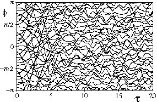
FIG. 1.: Quasienergy levels $\varphi$ of the kicked top with the Floquet operator $F(\tau)=e^{-i\beta J_{y}}e^{-i\alpha J_{x}}e^{-i\frac{\tau}{2j+1}J_{x^{2}}}$ for $j=15$, $\alpha=0.907$, $\beta=1.072$. As $\tau$ grows from 0 to $\sim 5$ the spectrum “relaxes” from level clustering to level repulsion, while the dynamics goes from integrable to chaotic.

FIG. 2.: $N$-dependence of the level collision “time” $\propto N^{-\nu}$ for a Hamiltonian $H(\tau)=H_{0}\cos\tau+H_{1}\sin\tau$ with $H_{0},H_{1}$ polynomials in $SU(3)$ generators. Such an $H(\tau)$ can correspond to either 2 or 3 classical freedoms.

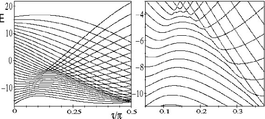
FIG. 3.: Level dynamics of the integrable spin Hamiltonian $H(\tau)\,=(J_{z}+0.4J_{x})\,{\rm cos}\,\tau+(\frac{4}{2j+1}J_{z}^{2}-0.5J_{z}-\frac{2j+1}{2})\,{\rm sin}\,\tau$ with $j=15$. Strongly avoided crossings are rare exceptions. Right box is a blow-up of left.

REFERENCES

- [1] O. Bohigas, M. J. Giannoni, C. Schmit, Phys. Rev. Lett. 52, 1 (1984)
- [2] M. V. Berry, Proc. R. Soc. London A413, 183 (1985)
- [3] H.-J. Stöckmann, Quantum Chaos (Cambridge University Press, 1999) and references therein
- [4] F. Haake, Quantum Signatures of Chaos (Springer, Berlin, 1991; 2nd ed. 2000) and references therein
- [5] M. L. Mehta, Random Matrices and the Statistical Theory of Energy Levels (Academic, New York, 1967; 2nd ed. 1991) and references therein
- [6] E. Bogomolny, B. Georgeot, M. J. Giannoni, C. Schmit, Phys. Rep. 291, 219 (1997)
- [7] J. P. Keating, F. Mezzadri, Nonlinearity 13, 747 (2000)
- [8] T. Yukawa, Phys. Rev. Lett. 54, 1883 (1985)
- [9] M. Wilkinson, J. Phys. A: Math. Gen. 21, 1173 (1988)
- [10] A. V. Andreev, B.L. Altshuler, Phys. Rev. Lett. 75, 902 (1995)
- [11] M.R. Zirnbauer in I.V. Lerner, J.P. Keating, D.E. Khmelnitskii (eds.), Supersymmetry and Trace Formulae; Chaos and Disorder (Kluwer Academic/Plenum, New York, 1999)
- [12] P. Pechukas, Phys. Rev. Lett. 51, 943 (1983)
- [13] F. Calogero, F. Marchioro, J. Math. Phys. 15, 1425 (1974); B. Sutherland, Phys. Rev. A5, 1372 (1972); J. Moser, Adv. Math. 16, 1 (1975); S. Wojciechowski, Phys. Lett. 111A, 111 (1985)
- [14] B. Dietz, F. Haake, Europhys. Lett. 9, 1 (1989)
- [15] H. Lipkin, N. Meshkov, A. J. Glick, Nucl. Phys. 62, 188 (1965); W. Wang, F. M. Izrailev, G. Casati, Phys. Rev. E57, 323 (1998) and references therein
- [16] S. Gnutzmann, F. Haake, M. Kuś, J. Phys. A33, 143 (2000)
- [17] F. Haake, H.-J. Stöckmann, Physikalische Blätter 56, 6, 27 (2000)
- [18] E. B. Bogomolny, U. Gerland, C. Schmit, Phys. Rev. E 59, R1315 (1999)