Chaotic Advection near 3-Vortex Collapse

Abstract

Dynamical and statistical properties of tracer advection are studied in a family of flows produced by three point-vortices of different signs. Tracer dynamics is analyzed by numerical construction of Poincaré sections, and is found to be strongly chaotic: advection pattern in the region around the center of vorticity is dominated by a well developed stochastic sea, which grows as the vortex system initial conditions are set closer to those leading to the collapse of the vortices; at the same time, the islands of regular motion around vortices, known as vortex cores, shrink. An estimation of the core’s radii from the minimum distance of vortex approach to each other is obtained. Tracer transport was found to be anomalous: for all of the three numerically investigated cases, the variance of the tracer distribution grows faster than a linear function of time, corresponding to a super-diffusive regime. The transport exponent varies with time decades, implying the presence of multi-fractal transport features. Yet, its value is never too far from 3/2, indicating some kind of universality. Statistics of Poincaré recurrences is non-Poissonian: distributions have long power-law tails. The anomalous properties of tracer statistics are the result of the complex structure of the advection phase space, in particular, of strong stickiness on the boundaries between the regions of chaotic and regular motion. The role of the different phase space structures involved in this phenomenon is analyzed. Based on this analysis, a kinetic description is constructed, which takes into account different time and space scalings by using a fractional equation.

I Introduction

The understanding of the advection of passive tracers is of fundamental interest for many different fields, ranging from a pure mathematical problem, to transport or mixing related ones. One area extensively studied in the last decade is the so called chaotic advectionAref84 -Crisanti92 . This phenomenon, resulting from a chaotic nature of Lagrangian trajectories, enhances the mixing of tracers in laminar flows, while in the absence of chaotic advection the mixing relies on the much less efficient mechanism of molecular diffusion.

Chaotic advection in geophysical flows is one of the important areas of application, where the advected quantities vary from the ozone in the stratosphere to various pollutants in the atmosphere and ocean, or such scalar quantities as temperature or salinity. The interest in the geophysical flows increases the practical significance of two-dimensional models and more specifically the advection in the system of vortices provenzale99 -Meleshko93 . In addition to the large scale geophysical flows, $2D$ decaying turbulence is another example, where the inverse cascade of energy generates coherent structures (vortices) which dominate the evolution of the flow Benzi86 -Carnevale91 . This type of problems represents only one facet of the interest inherent to the advection in few-vortices systems. Another facet is related to a transport of advected particles. It is known from different observations and numerous models, that the transport of advected particles is anomalous and, in one or another way, can be linked to the Levy-type processes and their generalizations Chernikov90 -Kovalyov2000 . Although these results pertain to fairly simple flows and models, there are speculations relating the chaotic advection in low-dimensional flows to particle dispersion in turbulent flows (see for example a discussion in zaslavsky93.2 ).

The interest to the chaotic advection in a three-vortex system is special not only for the reasons mentioned above. The three-vortex system is integrable, and its dynamics can be described in an explicit analytical form. An addition of a tracer (that can be regarded as another vortex of vanishing circulation) brings the number of particles in the system to four, which is a minimum number, from which the point vortex chaos begins Novikov78 ; ArefPomph80 ; the relative simplicity of the system permits to study anomalous transport in considerable detail. A discussion on the importance of three-vortex systems can be found in Aref99 .

In this article, we investigate dynamical and statistical properties of the advection in flows produced by three point vortices with different signs. For specific conditions on both the initial position of the vortices and their strength, the collapse of the three vortices to a single point is then possible. We first summarize the motivations for this work. It is known that for systems involving a large number of vortices, the local density of vortices fluctuates, these fluctuations are related to situations when few vortices are close to each other and form a cluster. The number of vortices included in theses cluster vary, but the typical number is around 2-3 Weiss98 ; Novikov75 ; Sire99 ; Zabusky96 , while cluster involving 4 vortices or more are much less probable. A given cluster exists only for a definite finite time $\Delta t$. During its existence, the notion of space-time structure of the cluster (or its configuration) can be introduced, and hence the influence of this structure on typical tracers motion and transport can be studied. Among different clusters, long time transport properties will be most influenced by clusters of vortices with the largest lifetime. The typical size of a cluster can be approximately defined by the minimum distance obtained between two vortices. The closer the vortices are to each other, the stronger is their mutual interaction and the longer the cluster lives. In order to change the inter-vortex distances it is necessary to consider a minimum of three-vortex interactions Aref79 ; Aref99 ; Novikov75 . And to bring all vortices close together (strong interaction) the configuration between the three vortices has to be close to to a configuration leading to a collapse of the vortices Zabusky96 . A typical lifetime estimation of these type of vortices can be assumed to be linked to the period of the motion of three vortices which are evolving on a close to collapse course. It is shown in this paper that the closer the vortices are to a collapse configuration the larger the period of the motion is, and that the growth of the period is exponential with respect to the closeness to the collapse configuration (see Appendix). We then expect that some clusters may have arbitrary long lifetime. Having in mind to shed some light on long time transport properties of systems involving many vortices, we decided to consider the simpler but nevertheless crucial case of transport properties in 3-vortex systems for close to collapse motion; this situations also provides an extreme situation best suited to test a possible universal transport property for three vortex flows. A simple way to define how close a motion is from the exact collapse course is through the deviations of the systems initial parameters from the conditions necessary for collapse. For instance one condition for collapse is $K=0$ (where $K$ is related to the angular momentum of the system), a close to collapse motion then necessarily satisfies $|K|=\varepsilon\ll 1$, and $\varepsilon$ is the “distance” from the collapse condition. Hence a special attention should be made to the notion of “close to collapse motion”, as in the whole paper we are referring as close for a small “distance” of the system in parameter space from the collapse conditions. And we insist that for “close to collapse” motions in the previous sense, no collapse of the vortices occurs and the minimum distance of approach between the vortices is finite. In this paper the motion of the vortices is chosen periodic, which retains the possibility of investigating long time transport properties of these types of flows. To conduct our study, we use the methodology and the results of our previous works. The dynamics of tracers is analyzed in a spirit similar to KZ98.1 , where the structure of the advection pattern (chaotic sea, resonant islands, stochastic layers, coherent cores, etc) was investigated numerically and analytically for the case of three identical vortices. Transport properties of the advection in that particular case (where no collapse or near-collapse vortex motion is possible) were found to be anomalous in KZ2000 . When vortex circulations have different signs, their dynamics may change considerably; the collapse phenomenon being one of the most striking examples. The motion of vortices in the vicinity of the collapse (when the collapse conditions are just slightly violated) was studied in LKZ2000 , where different routes in parameter space all leading to the collapse were outlined. While the kinetics of advected particles in non-collapsing three-vortex flows was described in KZ2000 , the situation with the advection in the near-collapse flows remained unclear. In this article we describe different topological structures of the advection pattern, depending on how far is the vortex system from the collapse conditions. We can speculate, that the characteristics of the transport of 3-vortex system can be extended to the case of many-vortex flows, since the advected particle finds itself quite often in the vicinity of a cluster of 3-4 vortices, that define the advection kinetics for a fairly long time-span. For our study, we chose three different cases, corresponding to a specific route to collapse: a far from collapse situation, an intermediate one, and one near the collapse. In these three cases the collapse of the vortices is never reached and the motion of the vortices is periodic, which allows the study of advection for large times and a better understanding of transport in three vortex flows, as we consider here an extreme case with bounded motion, namely the vicinity of collapse configuration.

In the Section 2, we present the basic equations of the point vortex dynamics, and discuss the collapse conditions in a three-vortex system. These results are based on the previous studies of the point vortex collapse Aref79 -Kimura90 . We use the notations introduced in LKZ2000 , and develop some argumentation related to our choice of approaching the initial configuration of the vortex system corresponding to the collapse configuration. Advection equations are introduced in the Section 3, where we present different tools used to investigate the dynamic properties of tracers. We focus on Poincaré sections, topology of the phase space, and trajectories, while in Section 4 we present different statistical results. They include velocity distributions, distributions of displacements and its moments, distribution of the Poincaré recurrences, etc. An important point of Section 4 is to understand better how the different regions of phase space influence the statistical properties of trajectories of advected particles.

On the basis of the obtained statistical information we consider kinetics of advected particles in Section 5. Fractional kinetics is involved in that description, and corresponding scalings and characteristic exponents are estimated on the basis of the results of Section 4. Motivation for the “3/2 law” of the transport is speculated, as well as the multi-fractal structure of kinetics. Finally, in the Conclusion we discuss different implications of the obtained results and a possibility to exploit them for the analysis of the advection in multi-vortex systems.

II Near-collapse vortex dynamics

The evolution of a system of $N$ point vortices can be described by a Hamiltonian system of $N$ interacting particles (see for instance Lamb45 ). The nature of the interaction depends on the geometry of the domain occupied by the fluid. For the case of an unbounded plane, the system’s evolution writes

$$k_{l}\dot{z}_{l}=-2i\frac{\partial H}{\partial\bar{z}_{l}}\>,\hskip 28.45274pt\dot{\bar{z}}_{l}=2i\frac{\partial H}{\partial(k_{l}z_{l})}\>,(l=1,\cdots,N)$$ (1)

with the Hamiltonian

$$H=-\frac{1}{2\pi}\sum_{l>m}k_{l}k_{m}\ln|z_{l}-z_{m}|=\frac{1}{4\pi}\ln\Lambda\>,$$ (2)

$z_{l}=x_{l}+iy_{l}$ is the complex coordinate of the vortex $l$, $k_{l}$ its strength and the couple $(k_{l}z_{l},\bar{z})$ are the conjugate variables of the Hamiltonian $H$, to whom a new energy parameter is associated

$$\Lambda\equiv e^{4\pi H}=\prod_{l\neq m}|z_{l}-z_{m}|^{k_{l}k_{m}}\>,$$ (3)

in order to simplify subsequent formulae.

The resulting complex velocity field $v$ is given by the sum of the individual vortex contributions:

$$v(z,t)=\frac{1}{2\pi i}\sum_{l=1}^{N}k_{l}\frac{1}{\bar{z}-\bar{z}_{l}(t)}.$$ (4)

When $z_{l}$ evolves according to (1), $v$ provides a solution of the two-dimensional Euler equation, describing the dynamics of a singular distribution of vorticity

$$\omega(z)=\sum_{l=1}^{N}k_{l}\delta\left(z-z_{l}(t)\right).$$ (5)

in an ideal incompressible two-dimensional fluid.

The motion equations (1) have, besides the energy, three other conserved quantities resulting from the translational and rotational invariance of $H$:

$$Q+iP=\sum^{N}_{l=1}k_{l}z_{l},\hskip 34.14322ptL^{2}=\sum_{l=1}^{N}k_{l}|z_{l}|^{2}.$$ (6)

It can be easily verified, that there are three independent first integrals in involution: $H$, $Q^{2}+P^{2}$ and $L^{2}$, from which it follows, that the motion of three vortices is always integrable. An analysis of possible regimes of the motion of three vortices and their classification can be found in Aref79 ; Tavantzis88 .

Among the different types of motion, there is an important special case known as vortex collapse. This motion is available when the sum of inverse vortex circulations (harmonic mean) is zero,

$$\sum^{3}_{l=1}\frac{1}{k_{l}}=0$$ (7)

and vortex positions positions are such, that the modified angular momentum $K$ computed in the reference frame for which the center of vorticity is placed at the origin, vanishes

$$K\equiv\left(\sum_{l=1}^{3}k_{l}\right)L^{2}-(Q^{2}+P^{2})=\sum_{l\neq m}^{3}k_{l}k_{m}|z_{i}-z_{j}|^{2}=0$$ (8)

Note, that the conditions (7) and (8) do not specify the motion uniquely, rather, they define a range of energies, for which the collapse is possible (once the values of $k_{l}$ satisfying (7) are given). When both of the conditions are satisfied, the solutions of (1) are singular and all three vortices collide at the center of vorticity in a finite time. Depending on the orientation of the vortex triangle, the collapse time $t_{c}$ can be either positive or negative. The first possibility, $t_{c}>0$, corresponds to an actual collapse, while for $t_{c}<0$ the vortex configuration expands without bounds. These two cases are exact images of each other under the time-reversal symmetry, and we refer to both of them as vortex collapse, keeping in mind, that for $t_{c}<0$ the collapse singularity lies backward in time. During the motion, the vortex configuration stays similar to the initial one, meanwhile the area of the triangle, formed by the three vortices grows/decreases linearly in time. We refer the reader to Aref79 ; Tavantzis88 ; LKZ2000 for more details.

When the collapse conditions (7,8) are satisfied only approximately, the motion has a specific “near-collapse” type characterized by an emergence of new scales of distances and velocities, which differ significantly from the initial ones LKZ2000 . A detailed analysis of the near-collapse dynamics of three vortices was performed in LKZ2000 for the case when two of the vortices have the same strength. A multitude of motion regimes was found in the vicinity of collapse; different regimes are distinguished by the way the collapse conditions (7,8) are violated, i.e. whether the combinations $\sum 1/k_{l}$ and $K$ are greater, less or equal to zero. Moreover, for some of these combinations, the motion type also depends on the energy $\Lambda$ of the vortex configuration; for example, when $\sum 1/k_{l}<0$ and $K>0$ there exist critical energies $\Lambda_{c_{1}}$ and $\Lambda_{c_{2}}$, such that in the range $\Lambda_{c_{1}}>\Lambda>\Lambda_{c_{2}}$ the motion has two branches of periodic motion, for $\Lambda=\Lambda_{c_{2}}$ the motion is aperiodic, and for $\Lambda>\Lambda_{c_{2}}$ there is only one periodic branch left. A classification of the near-collapse motion regimes, including the behavior of their length and time scales as the collapse is approached, can be found in LKZ2000 .

In order to carry out a detailed study of the advection for close to collapse situations, we restrict our consideration to a specific one-parameter family of near-collapsing vortex systems, defined as follows:

1. Only one of the collapse conditions, the strength condition (7), is violated; the second condition (8) is satisfied, i.e. $K=0$.

2. The two positive vortices are identical, by an appropriate choice of time units their strength can be put to 1; in other words, we fix $k_{1}=k_{2}=1$. The circulation of the third vortex is negative, $k_{3}\equiv-k$, ($k>0$). In this situation, the collapse happens, when the strength of the third vortex reaches a critical value $k=k_{c}\equiv 1/2$. The “distance” of the system from the collapse can be measured by the amount of the strength detuning $\delta$,

   $$\delta\equiv k_{c}-k=1/2-k$$ (9)

   We will be considering only the case $\delta>0$.

3. The energy of the vortex configuration $\Lambda$ is fixed to a constant value $\Lambda=0.9$.

The first two conditions ensure the relative vortex motion to be periodic, and the choice of energy is such, that in the approach to collapse ($\delta\rightarrow 0$), the maximum inter-vortex distance grows very slowly (no noticeable changes in the range of $\delta$ considered below) while the minimum inter-vortex distance rapidly approaches zero. It gives us a convenient “collapse in a box” setting, where vortices initially separated by a distance of order one, are brought arbitrary close (controlled by $\delta$) together, which may be of interest for studies of transport in many vortex-systems. For instance, the ability to bring vortices closer to each other by orders of magnitude makes these 3-vortex processes a dominant interaction mechanism in a rare gas of vortex patches Zabusky96 .

Before proceeding to the discussion of the advection, we will briefly summarize the results from LKZ2000 , pertaining to our case. The dynamics of a three-vortex system with two identical vortices can be mapped to a one-dimensional Hamiltonian system describing a motion of a particle of a unit mass and zero total energy in an effective potential, that depends on the strength of the third vortex $k$, and the constants of motion $\Lambda$ and $K$ (see appendix). The dynamical variable $X$ of this one-dimensional system is equal to the squared distance between the two positive vortices

$$X\equiv|z_{2}-z_{1}|^{2},$$ (10)

the other two distances, can be found from the expressions for $\Lambda$ and $K$. And in our special case ($K=0)$ the motion is confined between two single roots of the potential,

$$X_{min}<X<X_{max}\>,$$ (11)

where

$$X_{min}\equiv\left(\frac{1-k}{2k}\right)^{k/\delta}\Lambda^{-1/2\delta},\hskip 34.14322ptX_{max}\equiv\left(\frac{1}{2k}\right)^{k/\delta}\Lambda^{-1/2\delta}\>,$$ (12)

which implies that $X(t)$ is a periodic function of time, and consequently the other inter-vortex distances are too, i.e. the relative motion of vortices in our one-parameter family is always periodic.

As the collapse is approached ($k\rightarrow 1/2$, $\delta\rightarrow 0$), the motion tends to cover all length scales: $X_{min}\rightarrow 0$, $X_{max}\rightarrow\infty$, and its period diverges as

$$T\sim\frac{1}{\delta}\Lambda^{-1/2\delta}\>.$$ (13)

(see the appendix for the derivation). The influence of this behavior on the properties of advection is investigated in the next section.

III Dynamics of the advection

A passive particle (tracer) follows the flow according to the advection equation

$$\dot{z}=v(z,t)$$ (14)

where $z(t)$ represent the tracer trajectory, and $v$ is the velocity field. In the case of a point vortex system, the velocity field is given by Eq. (4). The incompressibility of the flow allows to write the advection equation (14) in a Hamiltonian form:

$$\dot{z}=-i\frac{\partial\Psi}{\partial\bar{z}},\hskip 34.14322pt\dot{\bar{z}}=i\frac{\partial\Psi}{\partial z}$$ (15)

where a stream function

$$\Psi(z,\bar{z},t)=-\frac{1}{2\pi}\sum_{l=1}^{3}k_{l}\ln|z-z_{l}(t)|$$ (16)

acts as a Hamiltonian. This system in non-autonomous, since the stream function depends on time through the vortex coordinates $z_{l}(t)$. The character of this dependence (periodic or not) is important for the further analysis. Below we will show, that although (16) is quasiperiodic, it can be made periodic by an appropriate coordinate transformation, which means, that the advection in our system has a 1 1/2 degrees of freedom Hamiltonian dynamics.

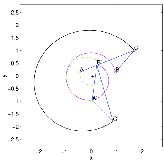
Figure 1: Vortex trajectories for $k=0.3$ in absolute reference frame. Initial vortex positions A,B (two positive vortices) and C (a negative one) are marked with circles. Vortex triangle $A^{\prime}B^{\prime}C^{\prime}$ corresponds to $t=t_{0}+T/2$, it is congruent to the initial $\Delta ABC$, but the two positive vortices are transposed; after another half-period of relative motion the original orientation restores. Center of vorticity is marked by a “+”.

Indeed, as was mentioned in the previous section, the relative vortex motion is periodic, i.e. the vortex triangle repeats its shape after a time $T$. This does not imply a periodicity of the absolute motion, since the triangle is rotated by some angle $\Theta$ during this time, see Fig. 1. In general, $\Theta$ is incommensurate with $2\pi$, rendering a quasiperiodic time dependence of $z_{l}(t)$.

Let us consider a reference frame, rotating around the center of vorticity with an angular velocity

$$\Omega\equiv\Theta/T.$$ (17)

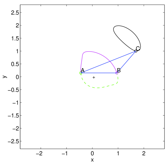
Figure 2: Same trajectories as in Fig. 1, plotted in the co-rotating frame: vortex motion is periodic.

In this co-rotating reference frame, vortices return to their original positions in one period of relative motion $T$, see Fig. 2, their new coordinates

$$\tilde{z}\equiv z\>e^{-i\Omega t}\>,$$

are periodic functions of time.

In the co-rotating frame the advection equation retains its Hamiltonian form with a new stream function $\tilde{\Psi}$ which acquires an extra (rotational energy) term

$$\tilde{\Psi}\equiv\Psi+\Omega^{2}/2|z|^{2}.$$ (18)

An advantage of this new frame is that $\tilde{\Psi}$ is time-periodic:

$$\tilde{\Psi}(\tilde{z},\tilde{\bar{z}},t+T)=\tilde{\Psi}(\tilde{z},\tilde{\bar{z}},t)$$ (19)

and well-developed techniques for periodically forced Hamiltonian systems can be used to study its solutions.

Note, that the one-period rotation angle $\Theta$ is defined modulo $2\pi$, making the choice of the co-rotating frame non-unique. We remove this ambiguity by requiring the negative vortex to make no full revolutions around the center of vorticity in the co-rotating frame (as in Fig. 2). This particular choice of $\Omega$ is inconsequential for the further analysis. The one-period rotation angles, relative motion periods and angular velocities of the co-rotating frame are presented in the Table 1. As the collapse is approached ($k\rightarrow 1/2$), $T$ grows rapidly (compare to the formula (13)), and the vortices make more and more turns per period, an acceleration of the rotation speed is also observed.

$k$	$0.2$	$0.3$	$0.41$
$\Theta(T)$	$-4.18\cdots\approx 2\pi/3-2\pi$	$-9.4\cdots\approx\pi-4\pi$	$-28.6\cdots\approx 0.9\pi-10\pi$
$T$	$10.71$	$17.53$	$36.86$
$\Omega_{v}=\Theta/T$	$-0.39$	$-0.54$	$-0.78$

Table 1: Different values of $\Theta(T)$ and the associated quantities, the relative period $T$ and the resulting apparent rotation speed.

We start our analysis of the advection by numerically constructing Poincaré sections of tracer trajectories (in the co-rotating frame). A Poincaré section is defined as an orbit of a period-one (Poincaré) map $\hat{P}$

$$\hat{P}z_{0}=\tilde{z}(T,z_{0})=e^{-i\Theta}z(T,z_{0})$$ (20)

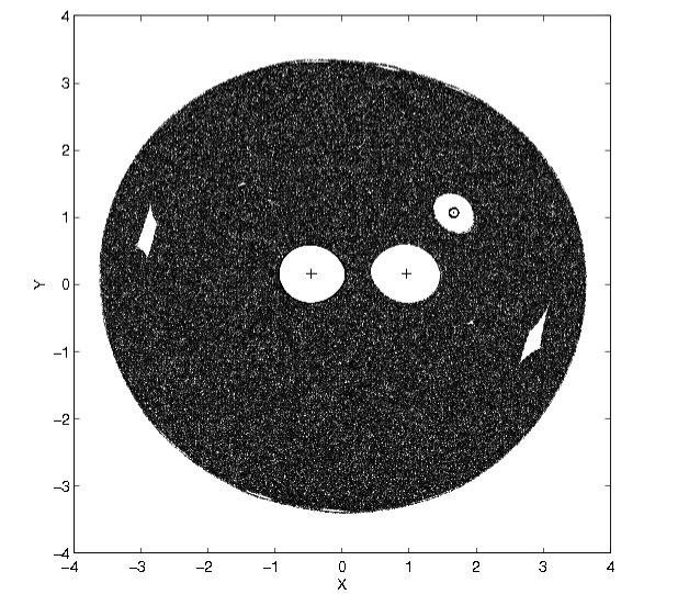
Figure 4: Poincaré Map of the system for the intermediate case. The constants of motion are $K=0$, $\Lambda=0.9$. Vortex strengths are $(-0.3,\>1,\>1)$. The period of the motion is $T=17.53$.

where $\tilde{z}(t,z_{0})$ denotes a solution $\tilde{z}(t)$ with an initial condition $\tilde{z}(t=0)=z_{0}$. Plots of Poincaré sections for three different values, $k=0.2$, $k=0.3$ and $k=0.41$ are shown in Figures 3-5. Vortex and tracer trajectories were computed using a symplectic fifth-order Gauss-Legendre scheme McLachlan92 . Exact conservation of Poincaré invariants by the symplectic scheme suppresses numerical diffusion, yielding high-resolution phase space portraits.

The Poincaré sections presented in Figures 3-5 show an intricate mixture of regions with chaotic and regular tracer dynamics, typical for periodically forced Hamiltonian systems. All three phase portraits share common features with the advection patterns, found in a flow due to three identical point vortices KZ98.1 ; NeufeldTel : the stochastic sea is bounded by a more or less circular domain, there are a number of islands inside it, where the tracer’s motion is predominantly regular. In particular, all three vortices are surrounded by robust near-circular islands, known as vortex cores. Contrary to the case of three identical vortices, where the tracer dynamics is integrable for a special value of vortex energy (when the vortices form a steadily rotating isosceles triangle) and has a near-integrable character in the vicinity, the tracer motion in the near-collapse flow family considered here is always strongly chaotic, the stochastic sea remains a principal element of the advection pattern for any $k$. The phase portraits indicate, that the degree of chaotization increases with the approach to collapse. For instance, in the far from collapse case $k=0.2$ the islands of regular motion inside the stochastic sea occupy a considerable area, and as $k$ increases, their share drastically diminishes.

A decrease in the radii of the vortex cores is of particular interest, since they are the robust structures, which also appear in many-vortex systems. The upper bound on the core radii can be obtained from the minimum approach inter-vortex distances. The minimum distance between the two positive vortices (see (12)) is

$$R_{1}^{min}=\left(\frac{1-k}{2k}\right)^{k/2\delta}\Lambda^{-1/4\delta}\>,$$ (21)

at the same moment the distance between the negative vortex and one of the positive two also reaches its minimum, which is

$$R_{2}^{min}=\frac{1}{2}\left(\sqrt{\frac{2-k}{k}}-1\right)R_{1}^{min}\>.$$ (22)

At this moment the vortices are collinear. Since the sum of the core radii of two vortices cannot exceed the minimum distance between them, we get an upper bound for the radius of the positive vortex core, $R^{+}_{core}$ and for that of the negative one, $R^{-}_{core}$, in terms of $R_{1}^{min}$, $R_{2}^{min}$:

$$R^{+}_{core}=\min\left(\frac{1}{2}R_{1}^{min},\frac{1}{1+\sqrt{k}}R_{2}^{min}\right)$$

$$R^{-}_{core}=\frac{\sqrt{k}}{1+\sqrt{k}}R_{2}^{min}$$ (23)

where we took into account, that the minimum distance between the positive and the negative vortex is shared between the corresponding cores depending on relative strength, and choose to define the boundary as the point between the two vortices with minimum speed. The core radii, measured directly from the phase portraits in Figures 3, 4, 5, and their upper bounds, obtained from (23) are listed in the Table 2.

	$k=0.2$	$k=0.3$	$k=0.41$
$r^{+}$	$\sim 0.51$	$\sim 0.43$	$\sim 0.16$
$r^{-}$	$\sim 0.3$	$\sim 0.2$	$\sim 0.1$
$R^{+}_{core}$	$0.69$	$0.57$	$0.19$
$R^{-}_{core}$	$0.43$	$0.31$	$0.12$
$R_{sea}$	$\sim 3.3$	$\sim 3.6$	$\sim 4$
$R_{1}^{max}$	$1.48$	$1.68$	$2.11$

Table 2: Comparison of the observed size of the vortex cores $r^{+}$, $r^{-}$ with their estimations $R^{+}_{core}$,$R^{-}_{core}$, given by 23; the external “radius” of the stochastic sea $R_{sea}$, and the maximum distance reached between identical vortices $R_{1}^{max}$.

The presence of islands where the motion is regular, in the stochastic sea, is known to alter the transport properties of a physical system. This phenomenon is known as “stickiness”; when a passive particle, traveling in the stochastic sea, gets close to an island, it is likely to stick to this island for a while and mimic a regular trajectory of a trapped particle. And since with each island, a whole hierarchy of smaller islands around islands is present, the particle can stick for arbitrary long times, which affects on the whole the transport properties of the system.

In KZ2000 , stickiness has been exhibited by measuring recurrence times of particles to a given part of phase space, and plotting the particles position on the map with a color accordingly to their return times. Particles, that have long return times, all stick to a particular island, and do not jump from one to another. Taking these facts into account, we use another way to visualize stickiness. Indeed, sticking particles have all long coherent time behavior, which reflects in quantities such as their angular speed, or intrinsic speed. We decide then to compute the average intrinsic speed over a definite amount of time of an ensemble of particles and record it. The measured quantity is the following

$$V_{i}(m,n)=\frac{1}{nT}\int^{t_{0}+n(m+1)T}_{t_{0}+nmT}v_{i}(t)dt\>,$$ (24)

where $n$ is the number of periods over which the speed is averaged, $m$ keeps track of the elapsed time, and $v_{i}(t)$ is the instantaneous speed at time $t$ of the particle $i$. We then define the distribution of such averaged velocities as

$$\rho(V;n,m)=\frac{1}{N_{p}}\sum_{i}\delta\left(V-V_{i}(m,n)\right)\>,$$ (25)

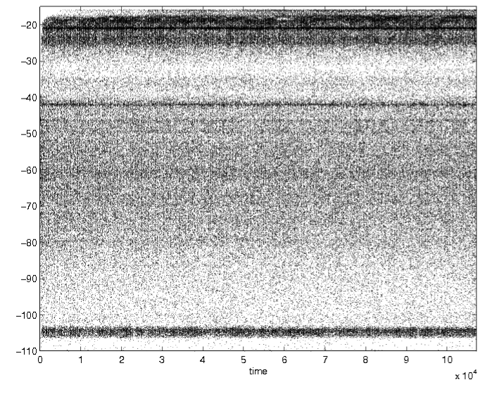
Figure 6: Averaged speed $V$ over $10$ periods versus time. We notice that some velocities are favored. The distribution does not seem to be time dependent except at the very beginning. The constants of motion are $K=0$, $\Lambda=0.9$. Vortex strengths are $(-0.2,\>1,\>1)$. The period of the motion is $T=10.73$.

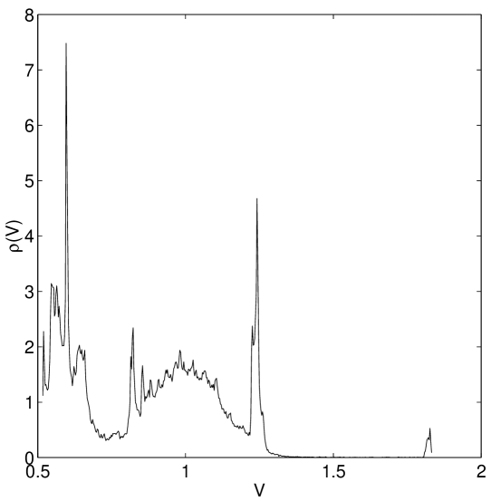
Figure 7: Probability distribution of $V=(s(t+10T)-s(t))/10T$, where $s$ is the arclength of a given tracer. We notice different peaks. The constant of motion are $K=0$, $\Lambda=0.9$. Vortex strengths are $(-0.2,\>1,\>1)$. The period of the motion is $T=10.726$.

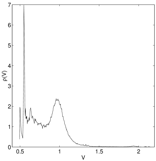
Figure 8: Probability distribution of $V=(s(t+10T)-s(t))/10T$. We notice different peaks. The constants of motion are $K=0$, $\Lambda=0.9$. Vortex strengths are $(-0.3,\>1,\>1)$. The period of the motion is $T=17.53$.

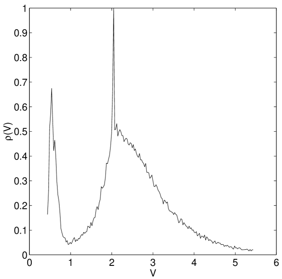
Figure 9: Probability distribution of $V=(s(t+10T)-s(t))/10T$. We notice different peaks. The constants of motion are $K=0$, $\Lambda=0.9$. Vortex strengths are $(-0.41,\>1,\>1)$. The period of the motion is $T=36.86$.

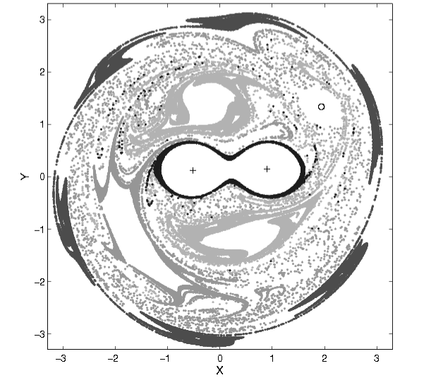
Figure 10: Location on the Poincaré section of the points with definite “special” averaged velocity (compare to peaks in Fig. 7). In dark gray the points corresponding to $0.595<V<0.605$. In light and lighter gray the points corresponding respectively to $0.81<V<0.83$ and to $1.22<V<1.25$. In black the points with corresponding speeds $V>1.8$. The constants of motion are $K=0$, $\Lambda=0.9$. Vortex strengths are $(-0.2,\>1,\>1)$. The period of the motion is $T=10.73$.

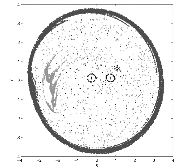
Figure 12: Location on the Poincaré section of the points with definite “special” angular velocity (compare to peaks in Fig. 9). In light gray the points corresponding to $0.7488<V<0.7515$. In black the points with corresponding speeds $V>1.5$. In dark gray the points corresponding to $V<0.489$ The constants of motion are $K=0$, $\Lambda=0.9$. Vortex strengths are $(-0.41,\>1,\>1)$. The period of the motion is $T=36.86$.

and smooth it over an interval to obtain a continuous curve. In fact, as can be observed in Fig. 6, for which the speed of particles is plotted versus time, we can notice that after a brief period of time the distribution seems stationary, meaning that $\rho(V,n,m)$ is independent of $m$ and therefore we can average its value over $m$, which in practice allows better statistics. Figure 6 is already informative, as we can notice some darker stripes, which means that some special average velocities are favored. This fits with the picture of some particles sticking to some island for a long time (at least $>10T$ here). To obtain this data we computed the trajectories over $10000$ periods for a sample of $253$ particles and recorded every $n=10$ periods. We use the stationarity property and plot the distribution $\rho$ versus the speed $V$ for the three different cases $k=0.2$, $0.3$, $0.41$, these are represented respectively in the figures Fig. 7, Fig. 8, and Fig. 9. We notice that the dark stripes observed in Fig. 6, correspond to peaks in the density probability. In order to characterize the origin of these peaks, we plotted in Fig. 10, Fig. 11, and Fig. 12, the position of the particles in the phase space contributing to the peaks in the distribution function. As anticipated, each of the observed peak correspond to a specific region of the phase space around some island. Concerning the influence of collapse, we notice that the area occupied by the contributing particles decreases as the critical condition is approached. We may then speculate that the transport properties of the three different system, which we discuss in the next section, may differ in a substantive way.

IV Anomalous statistical properties of tracers

Deterministic description of the motion of a passive particle in the mixing region is impossible, since a local instability produces exponential divergence of trajectories, and after a short time, the position of a tracer would be completely unpredictable. Even the outcome of an idealized numerical experiment is non-deterministic in this situation, since a round-off error is creeping slowly but steadily from the smallest to the observable scale. For this reason, long-time behavior of tracer trajectories in the mixing region is usually studied within a probabilistic approach.

In the absence of long-term correlations, a kinetic description, which uses Fokker-Plank-Kolmogorov equation and leads to Gaussian statistics, Zaslavsky92 works fairly well in many cases. Yet, in the present case, the complex topology of the advection pattern, illustrated by the Poincaré sections in Figures 3-5, indicates that one should anticipate anomalous statistical properties of the tracers in the chaotic sea. Singular zones around KAM islands usually produce long-time correlations, which may result in essential changes in the particle kinetics. Although in some cases these “memory effects” can be accounted for by the modification of the diffusion coefficient in the FPK equation Chirikov79 Rechester80 , often their influence is more profound Zaslavsky93 dCN98 Castiglione99 KZ2000 , and leads to a super-diffusive behavior with faster than linear growth of the particle displacement variance:

$$\langle(x-\langle x\rangle)^{2}\rangle\sim t^{\mu}$$ (26)

where the transport exponent $\mu$ exceeds the Gaussian value: $\mu>1$.

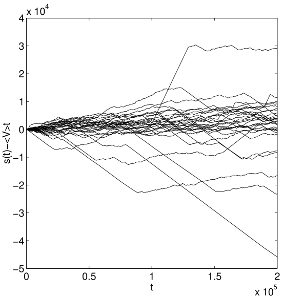
Figure 13: The deviation from the mean arclength ($s(t)-Vt$) versus time $t$ is plotted for $30$ particles. We notice the flights corresponding to a particle being in a the sticky zone around an island. The constants of motion are $K=0$, $\Lambda=0.9$. The run is over $20000$ periods. The average speed is $V\approx 0.87$. Vortex strengths are $(-0.2,\>1,\>1)$. The period of the motion is $T=10.73$.

In this section we analyze the statistical properties of tracers in the chaotic region for three vortex flow geometries, introduced above: far from collapse ($k=0.2$, Fig. 3), intermediate ($k=0.3$, Fig. 4), and close to collapse ($k=0.41$, Fig. 5). A plot of a time series of the arclength versus time $s_{i}(t)=\int v_{i}(t)dt$ for a set of typical tracers trajectories (Fig. 13) reveals an intermittent character of tracer motion: random pieces of trajectory are interrupted by regular flights, some of which are fairly long. To remain consistent with previous work, we focus our interest on the character of tracer rotation, and for that matter, we define its azimuthal coordinate in the center of vorticity reference frame

$$\theta(t)\equiv{\mbox{Arg}}\,\,z$$ (27)

to be a continuous function of time, i.e. $\theta(t)\in(-\infty,\infty)$ keeps track of the number of revolutions performed by a tracer.

Mean advection angle $\langle\theta(t)\rangle$ (here $\langle\,\,\rangle$ denotes ensemble average) grows linearly with time:

$$\langle\theta(t)\rangle=\omega t,$$ (28)

the values of the average rotation frequency $\omega$ for the three cases are listed in Table 3.

The growth of the variance,

$$\sigma^{2}(t)\equiv\langle(\theta(t)-\langle\theta(t)\rangle)^{2}\rangle$$ (29)

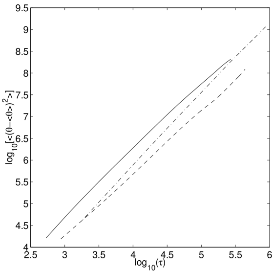
Figure 14: The second order moment for the angle distribution ($\langle(\theta(t)-\overline{\theta}(t))^{2}\rangle$) versus time for the three cases $k=0.2$ (solid line), $k=0.3$ (dashed line), and $k=0.41$ (dot-dashed line). We notice a change of behavior for the large times. The constants of motion are $K=0$, $\Lambda=0.9$.

is faster than linear for all three cases: angular tracer diffusion is anomalous. From log-log plots of $\sigma^{2}(t)$ versus time in Fig. 14, one may see, that in order to describe the growth of the variance with a power law

$$\sigma^{2}(t)\sim t^{\mu}$$ (30)

one has to introduce different transport exponents for different time ranges. The values of these exponents, obtained by linear fits of corresponding parts of the graphs of Fig. 14, are given in Table 3. Below, the first time range (with the exponent $\mu_{1}$) will be referred to as “short times”, and the second one ($\mu_{2}$) “long times”.

	$k=0.2$	$k=0.3$	$k=0.41$
$\omega$	$-0.484$	$-0.457$	$-0.387$
$\mu_{1}$	1.563	1.479	1.679
	$T<3\cdot 10^{4}$	$T<5\cdot 10^{4}$	$T<10^{5}$
$\mu_{2}$	1.226	1.707	1.589
	$T>10^{5}$	$T>1.5\cdot 10^{5}$	$T>5\cdot 10^{5}$

Table 3: Basic values of transport properties. The average rotation speed of the tracers and the exponent related to the time evolution of the second moment are given.

Recently Castiglione99 , two types of anomalous diffusion were distinguished by the behavior of the moments, other than variance. The case when the evolution of all of the moments can be described by a single self-similarity exponent $\nu$ according to

$$\langle|x-\langle x\rangle|^{q}\rangle\sim t^{q\nu}$$ (31)

was called “weak anomalous diffusion”, whereas the case when $\nu$ in (31) is not constant, i.e.

$$\langle|x-\langle x\rangle|^{q}\rangle\sim t^{q\nu(q)}$$ (32)

was named “strong anomalous diffusion”. The importance of this distinction comes from the fact, that in the weak case the PDF must evolve in a self-similar way:

$$P(x,t)=t^{-\nu}f(\xi),\hskip 28.45274pt\xi\equiv t^{-\nu}(x-\langle x\rangle)$$ (33)

whereas non-constant $\nu(q)$ in (32) precludes such self-similarity. Note, that a self-similar PDF evolution can have a more general form than (33), with $t^{-\nu}$ replaced by an arbitrary decaying function of time $g(t)$:

$$P(x,t)=g(t)f(g(t)(x-\langle x\rangle)),$$ (34)

which means, that if for different time decades $g(t)$ has different asymptotics, the self-similarity exponent $\nu$ will change from one decade to another. This variation of $\nu$ with time (in particular, differences of transport exponents for short and long times in Table 3) is not related to the type (strong or weak) of anomalous diffusion.

We have performed the measurements of a set of moments of tracer angular PDF (including non-integer values of $q$) defined as:

$$M_{q}(t)\equiv\langle|\theta(t)-\langle\theta(t)\rangle|^{q}\rangle$$ (35)

for the three vortex geometries. Time evolution of each moment was fitted by a power law:

$$M_{q}(t)\sim t^{\mu(q)}$$ (36)

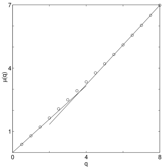
Figure 15: The exponent $q\nu(q)$ versus the moment order $q$ for the angle distribution ($\langle|\theta(t)-\overline{\theta}(t)|^{q}\rangle\sim t^{q\nu(q)}$) is plotted for the small times ($t<3\;10^{4}$, or $t<3000T$). We notice two linear behaviors: $\mu(q)=0.79q$ for $q<2$, and $\mu(q)=0.94q+Cte$ for $q>4$ Vortex strengths are $(-0.2,\>1,\>1)$. The period of the motion is $T=10.7$.

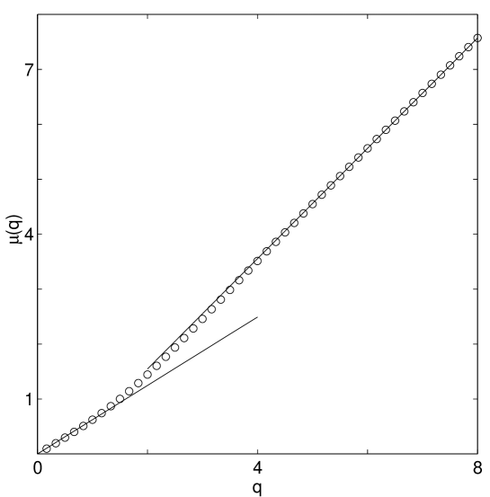
Figure 16: The exponent $\mu(q)$ versus the moment order $q$ for the angle distribution ($\langle|\theta(t)-\overline{\theta}(t)|^{q}\rangle\sim t^{\mu(q)}$) is plotted for the small times ($t<5\;10^{4}$, or $t<3000T$). We notice two linear behaviors: $\mu(q)=0.62q$ ($q<2$), $\mu(q)=1.00q+Cte$ ($q>2$). The constants of motion are $K=0$, $\Lambda=0.9$. Vortex strengths are $(-0.3,\>1,\>1)$. The period of the motion is $T=17.53$.

separately for short, and for long times. The results are summarized in Figures 15, 16, 17 (short times) and 18, 19, 20 (long times), where the exponents $\mu(q)$ are plotted versus the moment number $q$. In all cases, the apparent absence of a single linear fit indicates the presence of strong anomalous diffusion. This property was also found in KZ2000 (by comparison of the scaling properties of the central part of tracer PDF with the behavior of the variance) in a flow due to three vortices of equal strength. Thus, strong anomalous diffusion is a generic property of advection in three vortex flows.

Our results show, that $\mu(q)$ is well approximated by a piecewise linear function of the form:

$$\mu(q)=\left\{\begin{array}[]{ccc}\nu q&{\mbox{for}}&q<q_{c}\\ q-c&{\mbox{if}}&q>q_{c}\end{array}\right.$$ (37)

where $c$ is a constant, and $q_{c}$ is a crossover moment number $q_{c}=c/(1-\nu)$. In Castiglione99 , where this form was introduced, it was found, that it fits fairly well the numerically obtained values of $\mu(q)$ in all cases of strong anomalous diffusion, considered there, although a theoretical example of a system with arbitrary (concave) $\mu(q)$ was mentioned. Note, that deviations from (37), occurring in the crossover region $q\approx q_{c}$, are probably a result of finite observation time, and the form (37) might be precise in the limit $t\rightarrow\infty$.

As we have mentioned, the non-constant $\nu(q)$ in (32) is incompatible with the self-similar evolution of tracer distribution. Let us introduce an “almost self-similar distribution”

$$P(x,t)=\left\{\begin{array}[]{ccc}t^{-\nu}f(t^{-\nu}x)&{\mbox{for}}&x\ll vt\\ 0&{\mbox{if}}&x>vt\end{array}\right.$$ (38)

where the exact self-similarity (33) is broken only in the time-dependence of the cut-off. This modification of the exact self-similarity relation (33) takes into account the fact, that tracer speed is bounded by a maximum speed $v$. If $f(\xi)$ decays sufficiently fast at infinity (e.g. like a Gaussian), the cutoff behavior is irrelevant and the moments of (38) follow (31), but if $f(\xi)$ has a power tail, the almost self-similar distribution (38) will give the piecewise linear form (37) for the moments. If $f(\xi)\sim\xi^{-\beta}$ for large $\xi$, than low moments $M_{q}$ with $q<\beta-1$ will be determined by the central, self-similar part of the distribution, and high moments ($q>\beta-1$) by the cutoff value,

$$M_{q}(t)\sim\left\{\begin{array}[]{ccc}t^{\nu q}&{\mbox{for}}&q<\beta-1\\ t^{q-(1-\nu)(\beta-1)}&{\mbox{if}}&q>\beta-1\end{array}\right.$$ (39)

which is equivalent to (37) with

$$c=(1-\nu)(\beta-1)$$ (40)

We may conclude, that the piecewise linear dependence of the exponent $\mu(q)$ on the moment number $q$ is a signature of an almost self-similar evolution of tracer distribution with a long-tailed $f(\xi)$. The constant $c$ in (37) is related to the self-similarity exponent $\nu$ and power law decay exponent $\beta$ of $f(\xi)$ by (40).

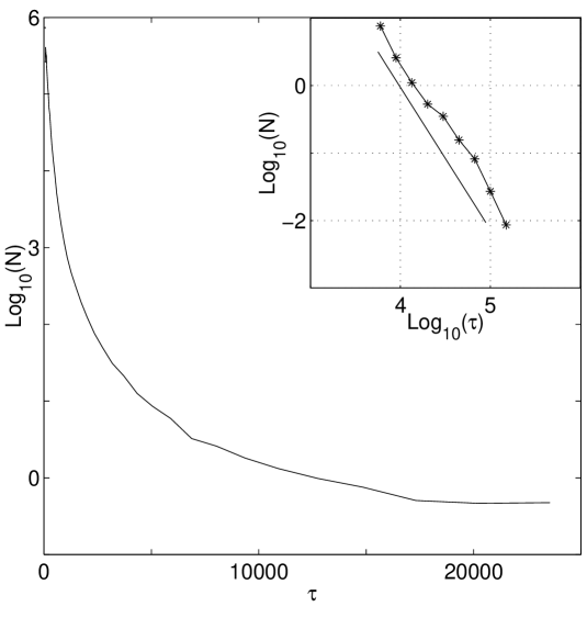
Figure 21: Distribution of Poincaré recurrences. The constants of motion are $K=0$, $\Lambda=0.9$. Vortex strengths are $(-0.2,\>1,\>1)$. The period of the motion is $T=10.7$. The tail presents a power law behavior whose exponent is $\sim 2.2$. The simulation is performed over 50 000 periods, statistics are made with 1137 particles.

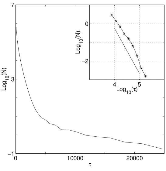
Figure 22: Distribution of Poincaré recurrences. The constants of motion are $K=0$, $\Lambda=0.9$. Vortex strengths are $(-0.3,\>1,\>1)$. The period of the motion is $T=17.53$. The tail presents a power law behavior whose exponent is $\sim 2.4$. The simulation is performed over 50 000 periods, statistics are made with 1012 particles.

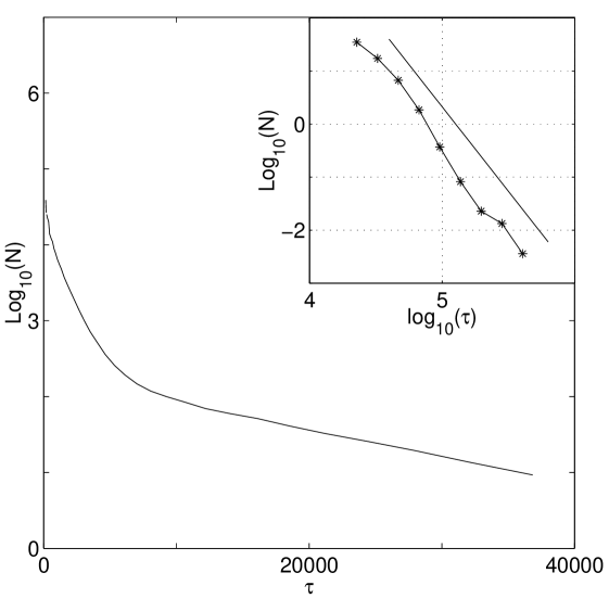
Figure 23: Distribution of Poincaré recurrences. The constants of motion are $K=0$, $\Lambda=0.9$. Vortex strengths are $(-0.41,\>1,\>1)$. The period of the motion is $T=36.85$. The tail presents a power law behavior whose exponent is $\sim 3.1$. The simulation is performed over 50 000 periods, statistics are made with 637 particles.

Another consequence of the intermittent character of tracer motion is an anomalous distribution of recurrences of the Poincaré map of tracer trajectories. To define recurrences, we take a region $B$ in the chaotic sea, and register all returns of a Poincaré map trajectory into $B$. The length of a recurrence is a time interval between two successive returns. In a system with perfect mixing, the PDF of recurrence lengths obeys a Poissonian law, provided $B$ is small enough, and decay of the long-recurrence tail of the distribution is exponential for any $B$. Recurrence distributions for tracers in all three cases ($k=0.2$, $k=0.3$ and $k=0.41$) are shown in Figures 21, 22, 23. The plots show, that all distributions have long tails, indicating, that between the returns tracers are being trapped in long flights of highly correlated motion. The form of the graphs suggests, that long recurrences are distributed according to a power law

$$P(t)\sim t^{-\gamma}$$ (41)

The values of the exponent $\gamma(\delta)$ are:

$$\gamma(0.2)=2.2\,\,\,\,\,\,\gamma(0.3)=2.4\,\,\,\,\,\,\gamma(0.41)=3.1\>.$$ (42)

Note, that while the collapse configuration is approached, the value of the exponent increases, which may be interpreted as an improvement in mixing properties of the flow. This agrees with the changes in the structure of Poincaré section (Fig. 10-12): the closer to collapse we get, the bigger part of the chaotic domain is occupied by a well-mixed area, and the smaller is the role of the singular zones around KAM islands.

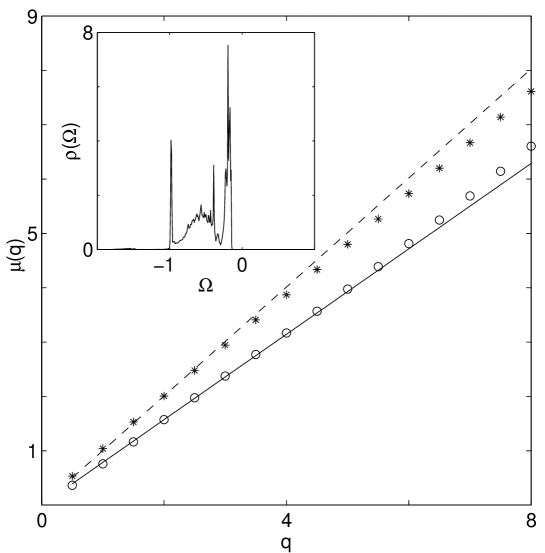
Figure 24: Exponents versus moment order in the case $k=0.2$, the difference with Fig.15 or Fig.18 is that here we did cut some parts of the distribution. the star sign “*” the slow motion (near zero peak corresponding to the outer rim) has been removed, the circle sign “o” the fast motion ($\Omega<-1$ corresponding to the cores) has been removed. We notice two linear behavior with slopes $0.78$ and $1$, which is respectively similar to the low and high moment behavior of Fig.15 or Fig.18. This allows us to identify the individual role in transport of the different structures in the phase space.

In fact one can try to find out the influence of the different islands on transport by using the distributions illustrated in Figures 7-9. Indeed, each island corresponds to a specific peak. We recompute the moments of the distribution in the far from collapse case $k=0.2$, for the modified data set, where the trajectories, corresponding to a specific peak are discarded. The result is presented in Fig. 24. We notice that the cores do affect the transport, but their influence is essentially visible for the high moments, while the slow particles trapped in the outer rim, are mainly responsible for the low moments; we also notice that we do not observe the change in slope of the strong anomalous behavior anymore, and conclude that the strong anomalous feature is due to the interplay of the different structures in the phase plane.

V Kinetics of advected particles

In some of the previous publications (see, for example, Chernikov90 ZEN97 -ZasEdel2000 ) it was clearly indicated that the properties of anomalous transport are sensitive to phase space topology. More specifically, if we use the fractional kinetic equation Zaslavsky92 ; ZEN97 in the form

$${\partial^{\beta}P(\theta,t)\over\partial t^{\beta}}={\mathcal{D}}{\partial^{\alpha}P(\theta,t)\over\partial|\theta|^{\alpha}}$$ (43)

to describe distributions $P(\theta,t)$ of rotations over angle $\theta$, then the transport coefficient $\mathcal{D}$ and exponents $(\alpha,\beta)$ depend on the presence of different structures such as boundaries of the domain, islands, cantori, etc. The results of Section 4 show the stickiness of trajectories of advected particles to the boundary of the domain and to boundaries of islands. This phenomenon is similar to what has been observed in KZ98.1 for the same-sign vortices. Our goal of this section is to estimate the values of the exponents $\alpha,\beta$.

Figures 10-12 demonstrate stickiness of trajectories to specific structures with a filamentation of sticky domains along stable/unstable manifolds. In fact, different sticky domains generate different intermittent scenarios with some associated values of $(\alpha,\beta)$ ZEN97 ; ZasEdel2000 . As a result, the real kinetics is multi-fractional and can be characterized by a set of values of $(\alpha,\beta)$ or, more precisely, by a spectral function of $(\alpha,\beta)$ in the same sense as the spectral function for multi-fractals Hentschel84 -Jensen85 . Figures 7-9 show that trajectories, sticking to different structures (islands), have different angular velocities (compare to peaks in Figures 7-9). Due to this, different asymptotics to the distribution function $P(\theta,t)$ and different values of $(\alpha,\beta)$ will appear for different time intervals. In other words, for a considered time interval one can expect a specific “intermediate asymptotics” for $P(\theta,t)$ and, correspondingly, different pairs $(\alpha,\beta)$. Different classes of universality for the values $(\alpha,\beta)$ were discussed in ZasEdel2000 . Below we will apply some of these results.

$k$	$q=2$	$q>2$
$0.2$	1.6	1.88
$0.3$	1.4	2.0
$0.41$	1.6	1.84

Table 4: Values of the transport exponents $\mu$ for different moments $q$.

Multiplying (43) by $|\theta|^{\alpha}$ and integrating it over $|\theta|$ we obtain

$$\langle|\theta|^{\alpha}\rangle\sim t^{\beta}$$ (44)

or, in the case of self-similarity the transport exponent $\mu$ from the equation

$$\langle|\theta|^{2}\rangle\sim t^{\mu}$$ (45)

can be estimated as

$$\mu=2\beta/\alpha$$ (46)

Expression (45) should be considered with some reservations since the second and higher moment may diverge. For a finite time $t<t_{\textrm{max}}$ particles reach a distance (angular rotation) $\theta<\theta_{max}$, which makes all moments finite. Typically all

$$\theta_{max}=\omega_{max}t$$ (47)

and $\omega_{max}$ (maximal angular velocity) can be reached only at the boundary of the domain of chaotic motion (see Figs. 6-8).

Using notations (31), (32), and

$$\mu(2)\equiv\mu$$ (48)

we can present the results for the transport exponents $\mu$ in Table 4. They are almost the same independently of how far is the control parameter $k$ from its critical value $k_{c}=1/2$ (the collapse condition). For large values of $q$ we have $\mu$ close to $\mu=2$ which corresponds to ballistic dynamics with $\alpha\approx\beta\approx 1$.

This result can be well understood from the stickiness of trajectories to the cores (see Figs. 10-12 in the black color). As it follows from distributions in Figs. 7-9, the particles that stick to the cores are the fastest ones, and they just define the large moments values.

The value of $\mu$ for $q=2$ is defined mainly by meso-structures in the middle of Figs. 10-12 (light gray). A typical property of these structures is existence of islands with well resolved filamentations due to the vicinity of the structures to a bifurcation. The latter is evident from the sharp corners of islands, which may indicate a parabolic type singular point Melnikov96 . A corresponding effective Hamiltonian, describing dynamics near a singular point, has a form Karney83 ; Melnikov96 ; ZEN97 ; Rom-Kedar99 :

$$H_{\textrm{eff}}=a_{1}(\Delta P)^{2}+a_{2}\Delta Q-Q_{3}(\Delta Q)^{3}$$ (49)

where $(P,Q)$ are generalized momentum and coordinate and $(\Delta P,\Delta Q)$ are their corresponding deviations from the singular point $(P_{0},Q_{0})$:

$$\Delta P=P-P_{0}\,\,,\,\,\,\,\,\,\,\,\Delta Q=Q-Q_{0}\,\,.$$ (50)

Particularly, it may be

$$Q=\theta\,\,,\,\,\,\,\,\,\,\,\,\,\,\,P=\dot{\theta}\,\,.$$ (51)

Depending on the coefficients $a_{j}$ and on the meaning of variables $(P,Q)$, which may be different from (51), one can describe singularity due to bifurcations for different types of dynamical modes: accelerator mode Karney83 ; Melnikov96 , “blinking island” mode Melnikov96 , ballistic mode Rom-Kedar99 , etc. For all these situations, universality of the Hamiltonian (49) permits estimation of the exponents $(\alpha,\beta)$ in (43)

A trajectory that approaches the vicinity of the singular point (or, simply, a corner of the island boundary), behaves intermittently and escapes the near-separatrix boundary layer. The phase volume of the escaping trajectories is

$$\delta\Gamma=\delta P\delta Q$$ (52)

where $\delta P,\delta Q$ are values $\Delta P,\Delta Q$ related to the escaping particles. From (49) we can estimate

$$\delta P_{\textrm{max}}\sim\delta Q^{3/2}$$ (53)

and from (52), (53)

$$\delta\Gamma\sim\delta Q^{5/2}$$ (54)

Escaping from the boundary layer means growth of the “radial” variable $\delta Q$ with time, i.e. for an initial time interval $\delta Q\sim t$, and consequently,

$$\delta\Gamma\sim t^{5/2}\>.$$ (55)

From (55) we conclude for the escape probability density to leave the boundary layer at time instant $t$ within interval $dt$:

$$\psi(t)\propto 1/\delta\Gamma\sim t^{-5/2}\,\,.$$ (56)

It was shown in Montroll84 that under special conditions the exponent $\gamma$ for the trapping time asymptotic distribution

$$\psi(t)\sim t^{-\gamma}$$ (57)

can be linked to fractal time dimension. Moreover, $\gamma$ is related to the kinetic equation (43) as ZEN97

$$\beta=\gamma-1\,\,.$$ (58)

For the considered case we have $\beta=3/2$.

For the spatial distribution of particles, the simplest situation occurs when the diffusion process has Gaussian type and, consequently, $\alpha=2$. In the case of the presence of hierarchical set of islands, $\alpha$ can be defined through scaling properties of the island areas. In the considered situation random walk is more or less uniform but trajectories are entangled near stable/unstable manifolds, i.e. in the light gray areas of Figs. 10-12. That means that $\alpha\sim 2$ although it is not exactly 2. Finally, we arrive to:

$$\mu=2\beta/\alpha\sim 3/2$$ (59)

in correspondence to observations in the Table 4. The value (59) was also discussed in ZasEdel2000 as one of possible universal values for the transport exponent $\mu$.

We need to comment that it is not worthwhile to try to obtain $\mu$ with a higher accuracy since a specific value of $\mu$ has no meaning due to multi-fractal nature of transport ZasEdel2000 . It is also important that we have considered such values of the control parameter $k$ for which there exists a strong filamentation. That guarantees a possibility of using Eq. (49) and the following analysis.

VI Conclusion

We have considered the dynamical and statistical properties of the passive particle advection in a family of flows, created by three point vortices of different signs. In all three particular cases, investigated numerically, tracer advection was strongly chaotic: advection patterns, visualized via Poincare sections of tracer trajectories are dominated by a well developed stochastic sea, occupying most of the area around the center of vorticity. With the approach of the vortex system to the collapse configuration, the degree of tracer chaotization increases: the stochastic sea grows, expanding outward and consuming some of the inner resonant islands.

The statistics of the tracers in the chaotic region is non-Gaussian. Anomalous diffusion (faster than linear growth of variance) with different time and space scales was found in all three cases, as well as non-Poissonian distributions of Poincaré recurrences (with power law decay of long recurrence probability). We did not find normal transport regimes, if such regime exist, they are confined to narrow windows in the parameter domain.

Transport anomalies are caused by the phenomenon of stickiness of the chaotic trajectories to the highly structured boundaries of the chaotic region. In the cases considered, three important types of boundaries can be distinguished: external border of the chaotic sea, boundaries of the resonant islands inside the chaotic sea, and boundaries of the vortex cores. Each of these influences various aspects of tracer statistics, analysis of their separate contributions shows, that the vortex cores, that rotate with the fastest rate, determine the high moments of the tracer distribution, while the external boundary, being the slowest, but the most sticky, dominate the low moments.

Vortex cores appeared in simulations Babiano ; NeufeldTel ; KZ98.1 , their origin and sizes were derived in KZ98.1 for a system of three identical vortices; particularly it was shown that the cores are the islands of stability filled by invariant curves and extremely thin stochastic layers. As the control parameter $k$ approaches the collapse value $k_{c}=1/2$, the sizes of the vortex cores noticeably decrease. An upper bound of the core radii, obtained from the minimum distance of vortex approach to each other, gives a good estimation for both positive and negative vortex core size.

Although the transport possesses multi-fractal features, it can be successively described by a fractional kinetic equation with characteristic exponents $\alpha\sim 2$ and $\beta\sim 3/2$. A corresponding moments dependence is

$$\langle|\theta|^{\alpha}\rangle\sim t^{\beta}\,\,.$$ (60)

The transport can be characterized by strong intermittency which manifests itself in strong deviation from (60) for higher moments, i.e.

$$\langle|\theta|^{2m}\rangle\sim t^{\mu(m)}$$ (61)

with $\mu\approx 3/2$ for $m=1$ and $\mu\approx 2m$ for large values of $m$. The latter corresponds to a strong influence of ballistic regime of tracer dynamics.

We note that the value $\beta\sim 3/2$ for $\alpha\sim 2$ has also been observed for flows generated by three identical vortices KZ2000 and since this value remains for 3-vortex flows with extreme stress (vicinity of collapse) we may reasonably speculate that for all periodic (bounded) three vortex flows $\beta\sim 3/2$. We would like to point out that the present work by analyzing the role played in transport by the different structures involved in the flow using various techniques, and by confirming a typical value of the second moment exponent should be of interest for the analysis of more realistic and complicated systems involving many vortices and coherent structures such as geophysical fluid dynamics.

Exponential Period Growth

In this appendix, we recall some earlier results presented in LKZ2000 , and compute an asymptotic of the period growth as a function of $\delta=1/2-k$.

It has been shown for the case of three vortices with two identical ones that the relative motion of these vortices can been described using an one-dimensional effective Hamiltonian

$$H_{eff}(\dot{X},X;\Lambda,K,k)\equiv P^{2}/2+V(X)=0\>,$$ (62)

with Hamiltonian equations

$$\dot{X}=\partial H_{eff}/\partial P\equiv P\>,\hskip 28.45274pt\dot{P}=-\partial H_{eff}/\partial X\>,$$ (63)

where $X=R^{2}_{1}$ is the square of the distance between the two positive vortices, and the potential $V$ has the following form

$$V(X)\equiv\frac{[(K-(1-k)X)^{2}-4k^{2}Y][(X-K)^{2}-4k^{2}Y]}{8\pi^{2}k^{2}Y^{2}}\>,\hskip 28.45274ptY=(\Lambda X)^{1/k}\>.$$ (64)

Let us now estimate the period of the relative motion in our case. In this paper we choose a situation with $K=0$, using then the transformation

$$U=X^{2}/4k^{2}Y\>,$$ (65)

the potential (64) becomes,

$$V(U)=\frac{2}{\pi^{2}}k^{2}\left(1-k\right)^{2}\left(U-\frac{1}{\left(1-k\right)^{2}}\right)\left(U-1\right)\>,$$ (66)

given the fact that $H_{eff}=0$, the motion is confined to the negative regions of the potential which leads to

$$1\leq U\leq\frac{1}{(1-k)^{2}}\>.$$ (67)

Consequently we obtain from (67) the boundaries for $X$ during the motion. We then compute the period of the relative motion using the effective potential

$$T=2\int^{X_{2}}_{X_{1}}\frac{dX}{\sqrt{-V(X)}}\>.$$ (68)

In the limit $\delta\rightarrow 0$ ($k\rightarrow 1/2$), we obtain

$$V(U)\sim\frac{1}{8\pi^{2}}(U-4)(U-1)\>,$$ (69)

and using the inverse transformation,

$$X=(4k^{2}\Lambda^{1/k}U)^{1/(2-1/k)}\sim(\Lambda^{2}U)^{-1/4\delta}\>,$$ (70)

we express the period in terms of $U$, which leads to

$$T\sim\frac{1}{4\delta}\int^{4}_{1}\frac{(\Lambda^{2}U)^{-1-1/4\delta}}{\sqrt{(U-1)(4-U)}}dU\>.$$ (71)

As $\delta\rightarrow 0$ ($k\rightarrow 1/2$), it is the numerator in (71), which defines the asymptotic behavior, since it is decreasing function of $U$, the dominant term is from $U=1$ which leads to

$$T\sim\frac{1}{\delta}\Lambda^{-1/2\delta}\>.$$ (72)

Since the condition $\Lambda=0.9<1$, is verified (and is necessary for the collapse to happen LKZ2000 ), we have an exponential growth of the period as the vortex-collapse configuration is approached.

Figure 3: Poincaré Map of the system for the far from collapse case. The constants of motion are $K=0$, $\Lambda=0.9$. Vortex strengths are $(-0.2,\>1,\>1)$. The period of the motion is $T=10.73$.

Figure 5: Poincaré Map of the system in the close to collapse case. The constants of motion are $K=0$, $\Lambda=0.9$. Vortex strengths are $(-0.41,\>1,\>1)$. The period of the motion is $T=36.86$.

Figure 11: Location on the Poincaré section of the points with definite “special” velocity (compare to peaks in Fig. 8). In light gray the points corresponding to $0.545<V<0.565$. In black the points with corresponding speeds $V>1.5$. In dark gray the points corresponding to $V<0.52$. The constants of motion are $K=0$, $\Lambda=0.9$. Vortex strengths are $(-0.3,\>1,\>1)$. The period of the motion is $T=17.53$.

Figure 17: The exponent $\mu(q)$ versus the moment order $q$ for the angle distribution ($\langle|\theta(t)-\overline{\theta}(t)|^{q}\rangle\sim t^{\mu(q)}$) is plotted for the short times ($t<10^{5}$). We notice two linear behaviors: $\mu(q)=0.78q$ ($q<2$), $\mu(q)=0.92q-Cte$ ($q>2$). The constants of motion are $K=0$, $\Lambda=0.9$. Vortex strengths are $(-0.41,\>1,\>1)$. The period of the motion is $T=36.85$.

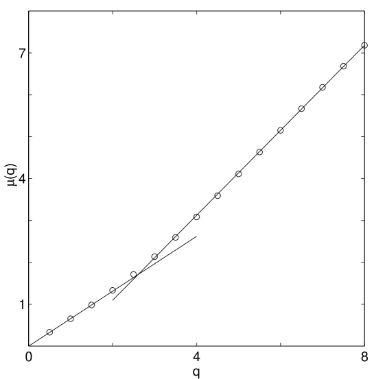
Figure 18: The exponent $\mu(q)$ versus the moment order $q$ for the angle distribution ($\langle|\theta(t)-\overline{\theta}(t)|^{q}\rangle\sim t^{\mu(q)}$) is plotted for the long times ($t>10^{5}$). We notice two linear behaviors: $\mu(q)=0.62q$ ($q<2$), $\mu(q)=1.01q-Cte$ ($q>2$). The constants of motion are $K=0$, $\Lambda=0.9$. Vortex strengths are $(-0.2,\>1,\>1)$. The period of the motion is $T=10.7$.

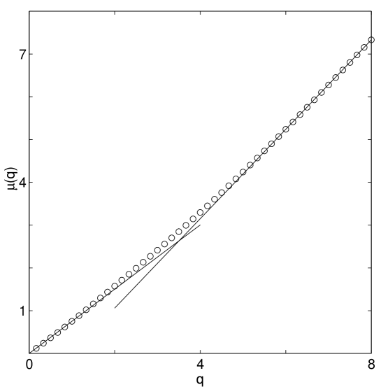
Figure 19: The exponent $\mu(q)$ versus the moment order $q$ for the angle distribution ($\langle|\theta(t)-\overline{\theta}(t)|^{q}\rangle\sim t^{\mu(q)}$) is plotted for the long times ($t>1.5\;10^{5}$). We notice two linear behaviors: $\mu(q)=0.75q$ ($q<2$), $\mu(q)=1.04q-Cte$ ($q>2$). The constants of motion are $K=0$, $\Lambda=0.9$. Vortex strengths are $(-0.3,\>1,\>1)$. The period of the motion is $T=17.53$.

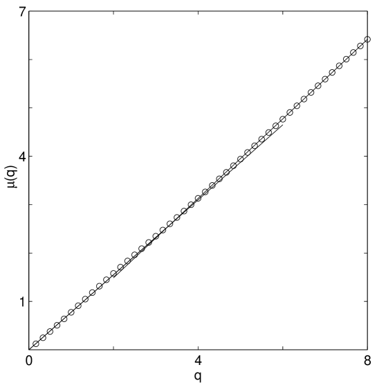
Figure 20: The exponent $\mu(q)$ versus the moment order $q$ for the angle distribution ($\langle|\theta(t)-\overline{\theta}(t)|^{q}\rangle\sim t^{\mu(q)}$) is plotted for the long times ($10^{6}>t>5\;10^{5}$). We notice two linear behaviors: $\mu(q)=0.77q$ ($q<2$), $\mu(q)=0.82q-Cte$ ($q>2$). The constants of motion are $K=0$, $\Lambda=0.9$. Vortex strengths are $(-0.41,\>1,\>1)$. The period of the motion is $T=36.85$.

References

- (1) H.Aref, Stirring by chaotic advection, J. Fluid Mech. 143, 1 (1984)
- (2) G. M. Zaslavsky, R. Z. Sagdeev, and A. A. Chernikov, Zhurn. Eksp. Teor. Fiz. 94, 102 (1988) (Soviet Physics, JETP 67, 270 (1988)
- (3) J. Ottino, The kinematics of Mixing: Stretching, Chaos, and Transport (Cambrige U. P., Cambrige, 1989)
- (4) H.Aref, Chaotic advection of fluid particles, Phil. Trans. R. Soc. London A 333, 273 (1990)
- (5) J. Ottino, Mixing, Chaotic advection and turbulence, Ann. Rev. Fluid Mech. 22, 207 (1990)
- (6) V. Rom-Kedar, A. Leonard and S. Wiggins, An analytical study of transport mixing and chaos in an unsteady vortical flow, J. Fluid Mech. 214, 347 (1990)
- (7) G. M. Zaslavsky, R. Z. Sagdeev, D. A. Usikov, and A. A. Chernikov, Weak Chaos and Quasiregular Patterns, Cambridge Univ. Press, (Cambridge 1991)
- (8) A. Crisanti, M. Falcioni, G. Paladin and A. Vulpiani, Lagrangian Chaos: Transport, Mixing and Diffusion in Fluids, La Rivista del Nuovo Cimento, 14, 1 (1991)
- (9) A. Crisanti, M. Falcioni, A. Provenzale, P. Tanga and A. Vulpiani, Dynamics of passively advected impurities in simple two-dimensional flow models, Phys. Fluids A 4, 1805 (1992)
- (10) A. Provenzale, Transport by Coherent Barotropic Vortices, Annu. Rev. Fluid Mech. 31, 55 (1999)
- (11) A. J. Majda, J. P. Kramer, Simplified models for turbulent diffusion: Theory, numerical modeling, and physical phenomena, Phys. Rep. 314, 238 (1999)
- (12) J. B. Weiss, A. Provenzale, J. C. McWilliams, Lagrangian dynamics in high-dimensional point-vortex system, Phys. Fluids 10, 1929 (1998)
- (13) J. C. McWilliams, J. B. Weiss and I Yavneh, The vortices of homogeneous geostrophic turbulence, J. Fuild Mech. 401, 1 (1999)
- (14) J. von Hardenberg, J. C. McWilliams, A. Provenzale, A. Shchepetkin and J. B. Weiss, Vortex merging in quasi-geostrophic flows, J. Fluid Mech. 412, 331 (2000)
- (15) P. Tabeling, A.E. Hansen, J. Paret, Forced and Decaying 2D turbulence: Experimental Study, in “Chaos, Kinetics and Nonlinear Dynamics in Fluids and Plasma”, eds. Sadruddin Benkadda and George Zaslavsky, p. 145, (Springer 1998)
- (16) A. E Hansen, D. Marteau , P. Tabeling, Two-dimensional turbulence and dispersion in a freely decaying system, Phys. Rev. E 58, 7261 (1998)
- (17) P. Tabeling, S. Burkhart, O. Cardoso, H. Willaime, Experimental-Study of Freely Decaying 2-Dimensional Turbulence, Phys. Rev. Lett. 67, 3772 (1991)
- (18) V.V. Meleshko, M.Yu. Konstantinov, Vortex Dynamics and Chaotic Phenomena, (World Scientific, Singapore, 1999)
- (19) R. Benzi, G. Paladin, S. Patarnello, P. Santangelo and A. Vulpiani, Intermittency and coherent structures in two-dimensional turbulence, J. Phys A 19, 3771 (1986)
- (20) R. Benzi, S. Patarnello and P. Santangelo, Self-similar coherent structures in two-dimensional decaying turbulence, J. Phys A 21, 1221 (1988)
- (21) J. B. Weiss, J. C. McWilliams, Temporal scaling behavior of decaying two-dimensional turbulence, Phys. Fluids A 5, 608 (1992)
- (22) A. Bracco, J. C. McWilliams, G. Murante, A. Provenzale, J. B. Weiss, Revisiting freely decaying two-dimensional turbulence at millennial resolution, Phys. Fluids 12 2931, (2000)
- (23) J. C. McWilliams, The emergence of isolated coherent vortices in turbulent flow, J. Fluid Mech. 146, 21 (1984)
- (24) J. C. McWilliams, The vortices of two-dimensional turbulence, J. Fluid Mech. 219, 361 (1990)
- (25) D. Elhmaïdi, A. Provenzale and A. Babiano, Elementary topology of two-dimensional turbulence from a Lagrangian viewpoint and single particle dispersion, J. Fluid Mech. 257, 533 (1993)
- (26) G. F. Carnevale, J. C. McWilliams, Y. Pomeau, J. B. Weiss and W. R. Young, Evolution of Vortex Statistics in Two-Dimensional Turbulence, Phys. Rev. Lett. 66, 2735 (1991)
- (27) A. A. Chernikov, B. A. Petrovichev, A. V. Rogal’sky, R. Z. Sagdeev, and G. M. Zaslavsky, Anomalous Transport of Streamlines Due to their Chaos and their Spatial Topology, Phys. Lett. A 144, 127 (1990)
- (28) T.H. Solomon, E.R. Weeks, H.L. Swinney, Chaotic advection in a two-dimensional flow: Lévy flights in and anomalous diffusion, Physica D, 76, 70 (1994)
- (29) E.R. Weeks, J.S. Urbach, H.L. Swinney, Anomalous diffusion in asymmetric random walks with a quasi-geostrophic flow example, Physica D, 97, 219 (1996)
- (30) G.M. Zaslavsky, D. Stevens, H. Weitzner, Self-similar transport in incomplete chaos, Phys. Rev E 48, 1683 (1993)
- (31) S. Kovalyov, Phase space structure and anomalous diffusion in a rotational fluid experiment, Chaos 10, 153 (2000)
- (32) G. M. Zaslavsky, How Long is the Way from Chaos to Turbulence?, in “New Approaches and Concepts in Turbulence”, eds. Th. Dracos and A. Tsinober, p 165 (Birkhäuser Verlag 1993)
- (33) E. A. Novikov, Yu. B. Sedov, Stochastic properties of a four-vortex system, Sov. Phys. JETP 48, 440 (1978)
- (34) H.Aref and N. Pomphrey, Integrable and chaotic motion of four vortices, Phys. Lett. A 78, 297 (1980)
- (35) A. Aref, P. L. Boyland, M. A. Stremler, and D. L. Vainchtein Turbulent Statistical dynamics of a system of point vortices, in “Trends in Mathematics”, p 151 (Birkhäuser Verlag 1999)
- (36) E. A. Novikov, Dynamics and statistics of a system of vortices, Sov. Phys. JETP 41, 937 (1975)
- (37) C. Sire and P. H. Chavanis, Numerical renormalization group of the vortex aggregation in 2D decaying turbulence: the role of three-body interactions. cond-mat/9912222 (1999)
- (38) D. G. Dritschel, N. J. Zabusky, On the nature of the vortex interactions and models in unforced nearly-inviscid two-dimensional turbulence, Phys. Fluids 8(5), 1252 (1996)
- (39) L. Kuznetsov and G.M. Zaslavsky, Regular and Chaotic advection in the flow field of a three-vortex system, Phys. Rev E 58, 7330 (1998)
- (40) L. Kuznetsov and G. M. Zaslavsky, Passive particle transport in three-vortex flow. To appear in Phys. Rev. E.
- (41) X. Leoncini, L. Kuznetsov and G. M. Zaslavsky, Motion of Three Vortices near Collapse, Preprint 1999
- (42) H. Aref, Motion of three vortices, Phys. Fluids 22, 393 (1979)
- (43) Z. Neufeld and T. Tél, The vortex dynamics analogue of the restricted three-body problem: advection in the field of three identical point vortices, J. Phys. A: Math. Gen. 30, 2263 (1997)
- (44) E. A. Novikov, Yu. B. Sedov, Vortex collapse, Sov. Phys. JETP 22, 297 (1979)
- (45) J. L. Synge, On the motion of three vortices, Can. J. Math. 1, 257 (1949)
- (46) J. Tavantzis and L. Ting, The dynamics of three vortices revisited, Phys. Fluids 31, 1392 (1988)
- (47) Y. Kimura, Parametric motion of complex-time singularity toward real collapse, Physica D 46, 439 (1990)
- (48) C. Machioro and M. Pulvirenti, Mathematical theory of incompressible nonviscous fluids, Applied Mathematical Science 96 (Springer-Verlag, New York, 1994)
- (49) P. Saffman, Vortex Dynamics, Cambridge Monographs on Mechanics and Applied Mathematics (Cambridge University Press, Cambridge, 1995)
- (50) R.I. McLachlan, P. Atela, The accuracy of symplectic integrators, Nonlinearity 5, 541 (1992)
- (51) G.M. Zaslavsky, in “Topological Aspects of the Dynamics of Fluids and Plasmas”, ed. H.K. Moffatt, et al, p. 481, (Kluwer, Dordrecht, 1992); Chaos 4, 25 (1994); Physica D 76, 110 (1994)
- (52) B. V. Chirikov, Phys. Rep. 52, 264 (1979)
- (53) A.B. Rechester, R. White, Phys. Rev. Lett. 44, 1586 (1980)
- (54) D. del-Castillo-Negrete, Asymmetric transport and non-Gaussian statistics of passive scalars in vortices in shear, Phys. Fluids 10, 576 (1998)
- (55) P. Castiglione, A. Mazzino, P. Muratore-Ginanneschi and A. Vulpiani, On strong anomalous diffusion, Physica D 134, 75 (1999)
- (56) S. Benkadda, S. Kassibrakis, R.B. White, G.M. Zaslavsky, Phys. Rev. E, 59, 3761 (1999)
- (57) G. M. Zaslavsky, and B. A. Niyazov, Phys. Rep. 283, 73 (1997)
- (58) G. M. Zaslavsky, M. Edelman, B. A. Niyazov, Self-similarity, renormalization, and phase space nonuniformity of Hamiltonian chaotic dynamics, Chaos 7, 159 (1997)
- (59) G. M. Zaslavsky and M. Edelman, Hierachical structures in the phase space and fractional kinetics: I classical systems, Chaos 10, 135 (2000)
- (60) H. G. E. Hentschel and I. Procaccia, Physica D 8, 435 (1983); P. Grassberger and I. Procaccia, ibid, 13, 34 (1984)
- (61) U. Frisch and G. Parisi, in Turbulence and Predictability of Geophysical Flows and Climate Dynamics, edited by M. Ghill, R. Benzi, and G. Parisi (North-Holland, Amsterdam, 1985)
- (62) M. H. Jensen, L. P. Kadanoff, A. Libshaber, I. Procaccia, and J. Stavans, Phys. Rev. Lett. 55, 439 (1985); T. C. Halsey, M. H. Jensen, L. P. Kadanoff, A. Libshaber, I. Procaccia, and B. I. Schraiman, Phys. Rev. A 33, 1141 (1986)
- (63) V. K. Melnikov, On the existence of self-similar structures in the resonnance domain, in Transport, Chaos and Plasma Physics II, Proceedings, Marseille, edited by F. Doveil, S. Benkadda, and Y. Elskens (World Scientific, Singapore, 1996), pp. 142-153
- (64) C. C. F. Karney, Physica D 8, 360 (1983)
- (65) V. Rom-Kedar and G. M. Zaslavsky, Islands of accelerator modes and homoclinic tangles, Chaos 9, 697 (1999)
- (66) E. W. Montroll and M. F. Shlesinger, in Studies in Statistical Mechanics, edited by J. Lebowitz and E. Montroll (North-Holland, Amsterdam, 1984), Vol. 11, p. 1
- (67) H. Lamb, Hydrodynamics, (6th ed. New York, Dover, 1945)
- (68) A. Babiano, G. Boffetta, A. Provenzale and A. Vulpiani, Chaotic advection in point vortex models and two-dimensional turbulence, Phys. Fluids 6, 2465 (1994)