Integrability and action operators in quantum Hamiltonian systems

Abstract

For a (classically) integrable quantum mechanical system with two degrees of freedom, the functional dependence $\hat{H}=H_{Q}(\hat{J}_{1},\hat{J}_{2})$ of the Hamiltonian operator on the action operators is analyzed and compared with the corresponding functional relationship $H(p_{1},q_{1};p_{2},q_{2})=H_{C}(J_{1},J_{2})$ in the classical limit of that system. The former is shown to converge toward the latter in some asymptotic regime associated with the classical limit, but the convergence is, in general, non-uniform. The existence of the function $\hat{H}=H_{Q}(\hat{J}_{1},\hat{J}_{2})$ in the integrable regime of a parametric quantum system explains empirical results for the dimensionality of manifolds in parameter space on which at least two levels are degenerate. The comparative analysis is carried out for an integrable one-parameter two-spin model. Additional results presented for the (integrable) circular billiard model illuminate the same conclusions from a different angle.

I Introduction

A conspicuous phenomenological discriminant between quantized integrable and nonintegrable parametric Hamiltonian systems with two or more degrees of freedom is the occurrence or prohibition of level crossings between states within the same invariant Hilbert subspace of the underlying symmetry group.Gutz90 ; Reic92 ; Gutz98 Consider a quantum system with $d$ continuous parameters whose classical counterpart is integrable on a manifold of dimensionality $d_{I}\leq d$ in parameter space. Empirical evidence suggests that level crossings occur on $(d_{I}-1)$-dimensional manifolds which are embedded in the integrability manifold. A recent study,SM98 which investigated this issue systematically, showed for a two-spin model with $d=6$ and $d_{I}=5$ that the level crossing manifolds are, in fact, four-dimensional and that they are all confined to the five-dimensional integrability manifold. It showed, moreover, that the (classical) integrability manifold can be reconstructed from the (intrinsically quantum mechanical) level crossing manifolds.

The focus of the present study is to illuminate the natural cause underlying this characteristic relationship between level crossing manifolds and integrability manifolds. We attribute this relationship to the presence of action operators as constituent elements of the Hamiltonian operator for integrable quantum systems.

The textbook solution of an integrable classical dynamical system with two degrees of freedom, specified by an analytic function $H(p_{1},q_{1};p_{2},q_{2})$ of canonical coordinates, is to transform the Hamiltonian into a function of two action coordinates: $H=H_{C}(J_{1},J_{2})$. The canonical transformation $(p_{i},q_{i})\to(J_{i},\theta_{i}),i=1,2$ to action-angle coordinates amounts to a solution of the dynamical problem because it transforms Hamilton’s equations of motion, $\dot{p}_{i}=-\partial H/\partial q_{i}$, $\dot{q}_{i}=\partial H/\partial p_{i}$, generically a set of coupled nonlinear differential equations, into $\dot{J}_{i}=0$, $\dot{\theta}_{i}=\partial H_{C}/\partial J_{i}\equiv\omega_{i}$ with the solutions $J_{i}={\rm const}$, $\theta_{i}(t)=\omega_{i}t+\theta_{i}^{(0)}$.

This solution is guaranteed whenever a second integral of the motion can be found, i.e. an analytic function $I(p_{1},q_{1};p_{2},q_{2})$ which is functionally independent of $H$ and has a vanishing Poisson bracket with $H$: $dI/dt=\{H,I\}=0$. Deriving the expressions $H_{C}(J_{1},J_{2})$ and $I_{C}(J_{1},J_{2})$ from $H$ and $I$ requires the use of separable canonical coordinates. Finding separable coordinates can be a difficult task even if the second invariant is known.

The functions $H_{C}(J_{1},J_{2})$ and $I_{C}(J_{1},J_{2})$ establish a pivotal link between an integrable classical system and a quantized version of it. Semiclassical quantization derives its raison d’être from the obvious fact that quantizing a functional relation is much less problematic if it involves only quantities such as $H,I,J_{1},J_{2}$ whose quantum counterparts are guaranteed to be commuting operators.

II Quantum versus quantized

In the context of this study, it is useful to distinguish and compare three versions of the same model system: (i) the quantum version, (ii) the classical version, and (iii) the (semiclassically) quantized version.

The primary version is the quantum model, specified by the Hamiltonian expressed as an operator valued function of a set of dynamical variables (position, momentum, spin, $\ldots$) The commutation relations of these operators and the metric of the associated Hilbert space along with the rules of quantum mechanics then determine, via the Heisenberg equation of motion, the time evolution of any observable quantity of interest.

The classical limit converts the Hamiltonian operator into the classical energy function, the commutator algebra of dynamical variables into the symplectic structure (the fundamental Poisson brackets), and the Heisenberg equation of motion for any operator into the Hamilton equation of motion for the corresponding classical quantity. These quantities, in turn, enable us to express the energy function as a classical Hamiltonian, i.e. as a function of canonical coordinates.

The quantization of a classical Hamiltonian system requires a prescription for translating the functional relations between classical dynamical variables into functional relations between corresponding operators. Semiclassical quantization is one neat and clean procedure applicable to all integrable classical systems. It borrows from classical mechanics the functional dependence, $\hat{H}=H_{C}(\hat{J}_{1},\hat{J}_{2})$, of the Hamiltonian on the action operators and postulates that the eigenvalue spectrum of the latter consists of equidistant levels spaced by $\hbar$:

$$\langle\hat{J}_{i}\rangle=\hbar\left(n_{i}+\frac{1}{4}\alpha_{i}\right),~{}~{}i=1,2$$ (1)

with integer $n_{i}$. The (integer) Maslov indices $\alpha_{i}$ are determined by the topology of the classical trajectories in phase space.Perc77 Semiclassical quantization thus makes specific predictions for the energy level spectrum of the quantized version of the model system at hand.

In general, the (semiclassically) quantized and the (primary) quantum energy level spectra of one and the same integrable model system do not coincide. The relationship between the two spectra will be investigated in Sec. III for an integrable two-spin model and in Sec. IV for the (integrable) circular billiard model.

III Two-spin model

We consider two quantum spins ${\bf\hat{S}}_{1},{\bf\hat{S}}_{2}$ of equal length $\sqrt{\sigma(\sigma+1)}$ $(\sigma=\frac{1}{2},1,\frac{3}{2},\ldots)$ interacting via a uniaxially symmetric exchange interaction:note1

$$\hat{H}=-\left(\hat{S}_{1}^{x}\hat{S}_{2}^{x}+\hat{S}_{1}^{y}\hat{S}_{2}^{y}\right)-\kappa\hat{S}_{1}^{z}\hat{S}_{2}^{z}.$$ (2)

The second integral of the motion, which follows from Noether’s theorem, is

$$\hat{I}=\hat{M}_{z}=\frac{1}{2}\left(\hat{S}_{1}^{z}+\hat{S}_{2}^{z}\right).$$ (3)

In the classical limit $\hbar\to 0$, $\sigma\to\infty$, $\hbar\sqrt{\sigma(\sigma+1)}=s$, the operators ${\bf\hat{S}}_{i}$ turn into 3-component vectors, ${\bf S}_{i}=s(\sin\vartheta_{i}\cos\varphi_{i}$, $\sin\vartheta_{i}\sin\varphi_{i}$, $\cos\vartheta_{i})$, and Eq. (2) then describes the energy function of an autonomous Hamiltonian system with two degrees of freedom and canonical coordinates $p_{i}=s\cos\vartheta_{i},~{}~{}q_{i}=\varphi_{i},~{}~{}i=1,2$.MTWKM87

III.1 Classical actions

Generically, the classical time evolution of this system is nonlinear and quasiperiodic. In the parameter range $0<\kappa<1$, the following relation between the integrals of the motion $H=E$ (energy), $I=M_{z}$ (magnetization) and a set of classical actions $J_{1},J_{2}$ can be inferred from the exact solution:SM90

$$J_{1}=2M_{z},~{}~{}J_{2}=\frac{1}{2\pi}\int_{0}^{\tau}dt\frac{z\dot{\zeta}}{1+\zeta^{2}},$$ (4)

$$z(t) \equiv \frac{1}{2}s(\cos\vartheta_{1}-\cos\vartheta_{2})=z_{0}{\rm sn}(\rho t,z_{0}/a),$$

$$\zeta(t) \equiv \tan(\varphi_{1}-\varphi_{2})=\frac{\rho z_{0}{\rm cn}(\rho t,z_{0}/a){\rm dn}(\rho t,z_{0}/a)}{E+\kappa[M_{z}^{2}-z_{0}^{2}{\rm sn}^{2}(\rho t,z_{0}/a)]},$$

$$z_{0}^{2} = z_{m}^{2}-\sqrt{z_{m}^{4}-c},~{}~{}a^{2}=z_{m}^{2}+\sqrt{z_{m}^{4}-c},$$

$$c = [(s^{2}-M_{z}^{2})^{2}-(E+\kappa M_{z}^{2})^{2}]/(1-\kappa^{2}),$$

$$z_{m}^{2} = M_{z}^{2}+\frac{s^{2}-\kappa E}{1-\kappa^{2}},~{}~{}\tau=\frac{4}{\rho}{\rm K}\left(\frac{z_{0}}{a}\right),~{}~{}\rho=\sqrt{1-\kappa^{2}}a,$$

where sn$(p,x)$, cn$(p,x)$, dn$(p,x)$ are Jacobian elliptic functions and K$(p)$ is a complete elliptic integral.SO87

For the case $\kappa=1$ with higher rotational symmetry, considerable simplifications occur in the classical time evolution. Both spins precess uniformly about the direction of the conserved vector ${\bf S}_{T}\equiv{\bf S}_{1}+{\bf S}_{2}$, and the precession rate is $\omega=|{\bf S}_{T}|$ for both spins. Equations (4) for the classical actions become

$$J_{1} = 2M_{z},$$ (5a)

$$J_{2} = \frac{4}{\pi}\int_{0}^{\pi/2a}\!\!dt\!\!\left[z^{2}-\frac{z^{2}s^{2}+M_{z}^{2}-z^{2}}{(1+\zeta^{2})(E+M_{z}^{2}-z^{2})}\right]\!,$$ (5b)

$$z(t) = z_{0}\sin at,~{}~{}\zeta(t)=\frac{az_{0}\cos at}{E+M_{z}^{2}-z_{0}^{2}\sin^{2}at},$$

$$z_{0}^{2} = \frac{1}{2}(s^{2}+E)\left[1-\frac{4M_{z}^{2}}{a^{2}}\right],~{}~{}a=\sqrt{2(s^{2}-E)},$$

and can be evaluated in closed form:

$$J_{1} = 2M_{z},$$ (6a)

$$J_{2} = -\sqrt{2(s^{2}-E)}+(s-M_{z}){\rm sgn}(s^{2}-E-2sM_{z})$$ (6b)

$$+ (s+M_{z}){\rm sgn}(s^{2}-E+2sM_{z}).$$

Inverting relations (6) yields a degree-two polynomial dependence of $E,M_{z}$ on $J_{1},J_{2}$:

$$I_{C}(J_{1},J_{2}) = M_{z}=\frac{1}{2}J_{1},$$ (7a)

$$H_{C}(J_{1},J_{2}) = E=s^{2}-\frac{1}{2}l_{c}^{2},$$ (7b)

where $l_{c}=J_{2}-|J_{1}|$ if $s|J_{1}|>s^{2}-E$ and $l_{c}=2s-J_{2}$ if $s|J_{1}|<s^{2}-E$.

III.2 Quantum actions

For the case $\kappa=1$, the exact quantum spectrum follows directly from the higher rotational symmetry of $\hat{H}$:

$$\langle\hat{H}\rangle_{Q}=\hbar^{2}\sigma(\sigma+1)-\frac{\hbar^{2}}{2}l(l+1),~{}\langle\hat{M}_{z}\rangle_{Q}=\frac{\hbar}{2}m,$$ (8)

where $l=0,1,\ldots,2\sigma$ is the quantum number of the total spin and $m=-l,-l+1,\ldots,+l$ that of its $z$-component. One set of quantum actions (1) has eigenvaluesnote2

$$\langle\hat{J}_{i}\rangle/\hbar\equiv J_{i}^{Q}=-\sigma,-\sigma+1,\ldots,+\sigma,$$ (9)

which are related to $l,m$ as follows:

$$J_{1}^{Q} = \sigma-l,~{}~{}J_{2}^{Q}=\sigma-l-m~{}~{}~{}(m\leq 0),$$ (10a)

$$J_{1}^{Q} = \sigma-l+m,~{}~{}J_{2}^{Q}=\sigma-l~{}~{}~{}(m\geq 0).$$ (10b)

The two quantum invariants expressed as explicit functions of action operators then read

$$H_{Q}(\hat{J}_{1},\hat{J}_{2})=\hat{H} = \frac{1}{2}\hbar^{2}\sigma(\sigma+1)+\frac{1}{2}{\rm min}(\hat{J}_{1},\hat{J}_{2})$$ (11a)

$$\times [\hbar(2\sigma+1)-{\rm min}(\hat{J}_{1},\hat{J}_{2})],$$

$$I_{Q}(\hat{J}_{1},\hat{J}_{2})=\hat{M}_{z} = \frac{1}{2}(\hat{J}_{1}-\hat{J}_{2}),$$ (11b)

where ${\rm min}(\hat{J}_{1},\hat{J}_{2})$ selects the action operator with the smaller eigenvalue.

While the functional dependence in (11) is again described by a degree-two polynomial, it is different from the functional dependence (7) found classically. The former cannot be reconciled with the latter by any canonical transformation, nor does the quantum spectrum converge uniformly toward the classical spectrum for $\sigma\to\infty$, as we shall see in Sec. III.3.1.

For the cases $0\leq\kappa<1$ we must calculate the $(2\sigma+1)^{2}$ eigenvalues of the two quantum invariants $\hat{H},\hat{M}_{z}$ by numerical diagonalization of $\hat{H}$ in the $4\sigma+1$ invariant subspaces of $\hat{M}_{z}$. From the numerical data for $\langle\hat{H}\rangle$, $\langle\hat{M}_{z}\rangle$, we can infer the correct assignment of action quantum numbers $\langle\hat{J}_{i}\rangle/\hbar$ to eigenstates by smoothly connecting the spectrum in parameter space to the known relations (11) for $\kappa=1$. The resulting data for $H_{Q}(\hat{J}_{1},\hat{J}_{2}),I_{Q}(\hat{J}_{1},\hat{J}_{2})$ can then be compared with the (semiclassically quantized) inverse classical relations (4), $H_{C}(\hat{J}_{1},\hat{J}_{2})$, $I_{Q}(\hat{J}_{1},\hat{J}_{2})$, to high precision albeit not analytically as in the case $\kappa=1$. Numerical results will be presented in Sec. III.3.2.

III.3 Quantum corrections to quantized actions

In some simple applications, the functions $H_{Q},I_{Q}$ are identical to the functions $H_{C},I_{C}$. Hence there are no such quantum corrections. If we take, for example, the two-spin model $\hat{H}=-\hat{S}_{1}^{z}\hat{S}_{2}^{z}$, then both classical invariants $E,M_{z}$ depend solely on the canonical momenta, and the latter are identified to be actions: $p_{i}=J_{i}$. Hence we have $E=-J_{1}J_{2},M_{z}=\frac{1}{2}(J_{1}+J_{2})$, which, upon semiclassical quantization with $\langle\hat{J}_{i}\rangle/\hbar=-\sigma,-\sigma+1,\ldots,+\sigma$, yields the exact quantum eigenvalue spectrum. This situation is exceptional. For all cases of (2) with $0\leq\kappa\leq 1$, quantum corrections do exist.

III.3.1 Exact results for $\kappa=1$

For the parameter setting $\kappa=1$, the functions $H_{Q}(\hat{J}_{1},\hat{J}_{2})$, $I_{Q}(\hat{J}_{1},\hat{J}_{2})$ as given by expressions (11) are to be compared to the semiclassical expressions $H_{C}(\hat{J}_{1},\hat{J}_{2})$, $I_{C}(\hat{J}_{1},\hat{J}_{2})$ inferred from the classical relations (7) with quantum actions (9). It turns out to be more practical to perform the comparison for the inverse functional relations. We substitute $\sigma(\sigma+1)$ for $s^{2}$ and the exact eigenvalues (8) for $E,M_{z}$ into the classical expressions (6). The result is a set of non-integer valued semiclassical action quantum numbers

$$J_{1}^{C} = m,$$ (12a)

$$J_{2}^{C} = \left\{\begin{array}[]{ll}0&m=l=0\\ 2\sqrt{\sigma(\sigma+1)}-\sqrt{l(l+1)}&|m|<m_{0}\\ |m|-\sqrt{l(l+1)}&|m|>m_{0},\end{array}\right.$$ (12e)

where $m_{0}=l(l+1)/2\sqrt{\sigma(\sigma+1)}$. An optimal match with the quantum actions (10) can be achieved if we subject (12) to two successive canonical transformations:

$$J_{1}{{}^{C}}^{\prime} = J_{1}^{C},$$

$$J_{2}{{}^{C}}^{\prime} = \left\{\begin{array}[]{ll}2\sqrt{\sigma(\sigma+1)}-|J_{1}^{C}|+J_{2}^{C}&J_{2}^{C}\leq 0\\ J_{2}^{C}&J_{2}^{C}>0,\end{array}\right.$$

$$J_{1}{{}^{C}}^{\prime\prime} = \left\{\begin{array}[]{ll}J_{2}{{}^{C}}^{\prime}-2\sqrt{\sigma(\sigma+1)}+\sigma+\frac{1}{2}&J_{1}{{}^{C}}^{\prime}\leq 0\\ J_{2}{{}^{C}}^{\prime}-2\sqrt{\sigma(\sigma+1)}+\sigma+J_{1}{{}^{C}}^{\prime}+\frac{1}{2}&J_{1}{{}^{C}}^{\prime}>0\end{array}\right.$$

$$J_{2}{{}^{C}}^{\prime\prime} = \left\{\begin{array}[]{ll}J_{2}{{}^{C}}^{\prime}-2\sqrt{\sigma(\sigma+1)}+\sigma+\frac{1}{2}-J_{1}{{}^{C}}^{\prime}&J_{1}{{}^{C}}^{\prime}\leq 0\\ J_{2}{{}^{C}}^{\prime}-2\sqrt{\sigma(\sigma+1)}+\sigma+\frac{1}{2}&J_{1}{{}^{C}}^{\prime}>0.\end{array}\right.$$

We thus arrive at the expressions

$$J_{1}{{}^{C}}^{\prime\prime} = \left\{\begin{array}[]{ll}\sigma+\frac{1}{2}&m=l=0\\ \sigma-\sqrt{l(l+1)}+\frac{1}{2}&m\leq 0\\ \sigma-\sqrt{l(l+1)}+\frac{1}{2}+m&m>0,\end{array}\right.$$ (16d)

$$J_{2}{{}^{C}}^{\prime\prime} = \left\{\begin{array}[]{ll}\sigma+\frac{1}{2}&m=l=0\\ \sigma-\sqrt{l(l+1)}-m+\frac{1}{2}&m\leq 0\\ \sigma-\sqrt{l(l+1)}+\frac{1}{2}&m>0.\end{array}\right.$$ (16h)

The deviations of the non-integer valued $J_{1}{{}^{C}}^{\prime\prime},J_{2}{{}^{C}}^{\prime\prime}$ from the integer valued $J_{1}^{Q},J_{2}^{Q}$ then describe the quantum corrections to the semiclassical actions.

Using $\sqrt{l(l+1)}-\frac{1}{2}=l+{\rm O}(l^{-1})$, we see at once that the genuinely quantum mechanical relations (10) and the semiclassical relations (16) are asymptotically equivalent at low energies (large $l$) for $\sigma\to\infty$. At high energies (small $l$), on the other hand, the two relations remain distinct no matter how large we choose the value of the spin quantum number $\sigma$.

To set the stage for the cases $0<\kappa<1$, we plot in Figs. 1(a) and 2(a) the eigenvalues of $\hat{H}$ versus those of $\hat{M}_{z}$ in representations with spin quantum numbers $\sigma=2$ and $\sigma=4$, respectively. The patterns of regularity and similarity in the arrays of points are a direct consequence of the smooth functional relations $H_{Q}(\hat{J}_{1},\hat{J}_{2})$, $I_{Q}(\hat{J}_{1},\hat{J}_{2})$. The map $(\langle\hat{H}\rangle,\langle\hat{M}_{z}\rangle)\to(J_{1}^{Q},J_{2}^{Q})$ from the plane of invariants to the action plane is provided by Eqs. (10) and produces the triangles in Figs. 1(b) and 2(b). These points form a perfect lattice with unit spacing.

 

 

Figure 1: (a) Eigenvalue $\langle\hat{H}\rangle$ (energy) versus eigenvalue $\langle\hat{M}_{z}\rangle$ (magnetization) as given in Eqs. (8) of all eigenstates of Hamiltonian (2) with $\kappa=1$, $\sigma=2$. (b) The full triangles are the quantum images $(J_{1}^{Q},J_{2}^{Q})$ of these eigenstates in the action plane as provided by Eqs. (10). The open circles are the semiclassical images $(J_{1}{{}^{C}}^{\prime\prime},J_{2}{{}^{C}}^{\prime\prime})$ as provided by Eqs. (16) with $s^{2}=\sigma(\sigma+1)$.

 

 

Figure 2: Plot of the same quantities as in Fig. 1 but for spin quantum number $\sigma=4$.

If we use instead the map (16) provided by semiclassical quantization, we obtain the array of open circles in Fig. 1(b) and Fig. 2(b). The bonds shown in parts (a) and (b) of the two graphs correspond to each other. The distortion in the lattice of circles relative to the perfect lattice of triangles is a graphical representation of the quantum corrections in the functions $H_{Q}(\hat{J}_{1},\hat{J}_{2})$, $I_{Q}(\hat{J}_{1},\hat{J}_{2})$ relative to the semiclassical functions $H_{C}(\hat{J}_{1},\hat{J}_{2})$, $I_{C}(\hat{J}_{1},\hat{J}_{2})$. It visually confirms what we have already concluded from comparing (10) and (16), namely that the deviations die out at low energies (lower left area) but persist at high energies (upper right area) for $\sigma\to\infty$. A useful measure of the leading quantum correction to the semiclassical relation $H_{C}(\hat{J}_{1},\hat{J}_{2})$ is the quantity $\sigma\Delta J$, where

$$\Delta J\equiv\sqrt{(\Delta J_{1})^{2}+(\Delta J_{2})^{2}},\quad\Delta J_{i}\equiv J_{i}^{Q}-J_{i}{{}^{C}}^{\prime\prime}$$ (17)

represents the distance between the triangles and circles on corresponding array sites in Figs. 1(b) and 2(b). From Eqs. (10) and (16) we obtain

$$\Delta J=\left\{\begin{array}[]{ll}1/\sqrt{2}&l=0\\ \sqrt{2}\left(l-\frac{1}{2}-\sqrt{l(l+1)}\right)&l\neq 0\end{array}\right.$$ (20)

The dependence of $\sigma\Delta J$ on $J_{1}^{Q},J_{2}^{Q}$ thus represents the $1/\sigma$ quantum correction to the semiclassically quantized actions. It has an inverse first power divergence in one corner of the action plane for energy levels at the upper threshold of the spectrum: $\sigma\Delta J\sim[4\sqrt{2}(l/\sigma)]^{-1}$. For states with $l/\sigma\ll 1$ the leading quantum correction is of O(1). In this part of the spectrum, semiclassical quantization remains inadequate no matter how large we choose the spin quantum number $\sigma$.

The state with the largest quantum correction to semiclassical quantization is the singlet combination of the two spins. This state or any nearby state in the action plane have no proper semiclassical representation.

III.3.2 Numerical results for $0<\kappa<1$

 

 

Figure 3: (a) Eigenvalue $\langle\hat{H}\rangle$ (energy) versus eigenvalue $\langle\hat{M}_{z}\rangle$ (magnetization) of the $(2\sigma+1)^{2}=25$ eigenstates of the two-spin model (2) with $\kappa=0.1$ for $\sigma=2$. Data from a numerical diagonalization. (b) The full triangles are the eigenvalues $J_{i}^{Q}=\langle\hat{J}_{i}\rangle/\hbar$ of the action operators, the images of the inverted functions $H_{Q}(\hat{J}_{1},\hat{J}_{2})$, $I_{Q}(\hat{J}_{1},\hat{J}_{2})$. The open circles are the semiclassical images $(J_{1}{{}^{C}}^{\prime\prime},J_{2}{{}^{C}}^{\prime\prime})$ from Eqs. (4) with $s^{2}=\sigma(\sigma+1)$, the images of the inverted functions $H_{C}(\hat{J}_{1},\hat{J}_{2})$, $I_{C}(\hat{J}_{1},\hat{J}_{2})$.

Here we use the same graphical representation even though we must rely on the results of a numerical diagonalization for the energy eigenvalues. At $\kappa<1$ we observe that certain features of the quantum invariants change qualitatively because the rotational symmetry of $\hat{H}$ has been reduced, whereas other features remain qualitatively the same because the integrability of the model has not been destroyed.

 

 

Figure 4: Plot of the same quantities as in Fig. 3 but for spin quantum number $\sigma=4$.

In Figs. 3(a) and 4(a) we have plotted the eigenvalues $\langle\hat{H}\rangle$, $\langle\hat{M}_{z}\rangle$ of the two quantum invariants versus each other at $\kappa=0.1$ for $\sigma=2$ and $\sigma=4$, respectively. Again the data points display regular patterns. They evolve from the patterns shown in Figs. 1(a) and 2(a) by smooth deformation of the lines of bonds as the value of $\kappa$ is lowered gradually. The lower symmetry removes the level degeneracies pertaining to the strings of horizontal bonds in Figs. 1(a) and 2(a).

When we substitute the eigenvalues $\langle\hat{H}\rangle$ and $\langle\hat{M}_{z}\rangle$ from the numerical diagonalization into the exact expression (4) for the classical actions and subject the resulting set of discrete values $J_{i}^{C}$ to the transformations $J_{i}^{C}\to J_{i}{{}^{C}}^{\prime}\to J_{i}{{}^{C}}^{\prime\prime}$, we obtain arrays of points in the form of distorted lattices as illustrated by the open circles in Figs. 3(b) and 4(b) for the two examples at hand. The deviations of these data points from the sites of a perfect lattice (marked by triangles) then again represent the quantum corrections to the (semiclassically) quantized actions. The patterns in Figs. 3(b) and 4(b) are also connected to those in Figs. 1(b) and 2(b) by smooth deformation of the lines of bonds upon gradual variation of the parameter $\kappa$.

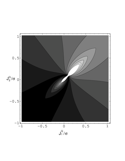
A closer look at the $1/\sigma$ quantum correction is afforded if we plot the scaled distance $\sigma\Delta J$ versus the scaled action quantum numbers $J_{1}^{Q}/\sigma$ and $J_{2}^{Q}/\sigma$ for a system with many more levels $(\sigma=40)$. A contour plot of the resulting landscape is shown in Fig. 5. Convergence of $\sigma\Delta J$ toward a smooth function of $J_{1}^{Q}/\sigma,J_{2}^{Q}/\sigma$ is almost uniform. In the case $\kappa=0.1$ considered here, there are two points (as opposed to a single corner point at $\kappa=1$), where the $1/\sigma$ correction diverges. The data points $\sigma\Delta J$ closest to these locations again tend to grow $\propto\sigma$.

Figure 5: Scaled distance $\sigma\Delta J$ for $\sigma=40$, $\kappa=0.1$ between the images of the inverted functions $H_{Q}(\hat{J}_{1},\hat{J}_{2})$, $I_{Q}(\hat{J}_{1},\hat{J}_{2})$ and the images of the inverted functions $H_{C}(\hat{J}_{1},\hat{J}_{2})$, $I_{C}(\hat{J}_{1},\hat{J}_{2})$.

The two sharply peaked maxima in the landscape of Fig. 5 will merge into a single divergence as $\sigma\to\infty$. At this point in the action plane, the leading quantum correction to semiclassical quantization is again of O(1). Its location in the action plane does, however, no longer coincide with an extremum in the energy level spectrum. The divergence in $\sigma\Delta J$ occurs at energy $E=\kappa s^{2}$ (for $\sigma\to\infty$), where the classical equations of motion have a fixed point. For eigenstates with action quantum numbers in the vicinity of this point, quantum effects persist no matter how large $\sigma$ is made.

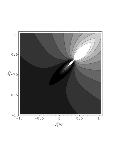
One point in the action plane where $\sigma\Delta J$ diverges exists throughout the regime $0\leq\kappa<1$. With $\kappa$ increasing from zero, the singularity moves gradually toward one corner of the action plane, and the energy of the state pertaining to those action coordinates moves toward the upper threshold of the spectrum. This trend is indicated in Fig. 6, which shows the $1/\sigma$-landscape for $\kappa=0.5$. The endpoint of this gradual shift, the case $\kappa=1$, was described in Sec. III.3.1.

 

Figure 6: Scaled distance $\sigma\Delta J$ for $\sigma=40$, $\kappa=0.5$ between the images of the inverted functions $H_{Q}(\hat{J}_{1},\hat{J}_{2})$, $I_{Q}(\hat{J}_{1},\hat{J}_{2})$ and the images of the inverted functions $H_{C}(\hat{J}_{1},\hat{J}_{2})$, $I_{C}(\hat{J}_{1},\hat{J}_{2})$.

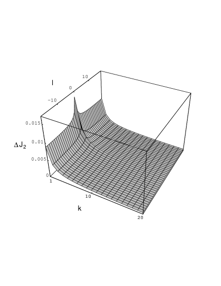
The asymptotic landscape for $\sigma\to\infty$ to which the graphs in Figs. 5 and 6 converge almost everywhere can now be used as the reference frame for the higher-order quantum corrections. The deviations of the data points from this new reference, appropriately scaled, will produce another landscape, representing the $1/\sigma^{2}$ correction to the semiclassically quantized actions.note3

We consider the line $J_{2}^{Q}=J_{1}^{Q}-\sigma/2$ for this purpose. In the main plot of Fig. 7 we show the $1/\sigma$ corrections $\sigma\Delta J$ along this line for $\sigma=4,8,16,32$. Also shown are data for $\sigma=1600$, which are very close to the asymptotic values for the $1/\sigma$ correction and now serve as the reference line for the $1/\sigma^{2}$ corrections.

In the inset to Fig. 7 we have plotted the scaled deviations of the $\sigma=4,8,16,32$ data from the new reference line. The results suggest that these data again converge toward a line, which will then be the reference line for $1/\sigma^{3}$ corrections. Like the reference line in the main plot of panel (a) [panel (b)], which is embedded in the landscape Fig. 5 [Fig. 6], the new reference line will be embedded in a landscape representing the $1/\sigma^{2}$ quantum corrections to semiclassical quantization over the entire action plane.

The point to be emphasized here is not the exact shape of the landscapes that represent successive orders of quantum corrections to the semiclassically quantized actions, but that such corrections exist and that the leading term may be of O(1) at special points rather than of O($\sigma^{-1}$) as might be expected.

 

 

Figure 7: Dependence of the scaled distance $\sigma\Delta J$ for (a) $\kappa=0.1$, (b) $\kappa=0.5$ between the images of the inverted functions $H_{Q}(\hat{J}_{1},\hat{J}_{2})$, $I_{Q}(\hat{J}_{1},\hat{J}_{2})$ and the images of the inverted functions $H_{C}(\hat{J}_{1},\hat{J}_{2})$, $I_{C}(\hat{J}_{1},\hat{J}_{2})$. Shown are data for $\sigma=4$ (squares), $\sigma=8$ (circles), $\sigma=16$ (triangles), $\sigma=32$ (pentagons), and $\sigma=1600$ (solid line). Inset: Scaled deviation $\sigma[\sigma\Delta J^{ref}-\sigma\Delta J^{\sigma}]$ of the $\sigma=4,6,8,16$ data from the reference line ($\sigma=1600$ data).

IV Circular Billiard

In the second application we consider a particle of mass $m$ that is free to move two-dimensionally across a circular area of radius $R$. The classical Hamiltonian expressed in polar canonical coordinates reads

$$H(p_{r},r;p_{\vartheta},\vartheta)=\frac{p_{r}^{2}}{2m}+\frac{p_{\vartheta}^{2}}{2mr^{2}}+V(r),$$ (21)

where $V(r)$ is a hard-wall potential that confines the particle to $r\leq R$.

In a recent study, Ree and ReichlRR98 analyzed this system classically and quantum mechanically as an integrable limiting case of the circular billiard with a straight cut. In general, the cut renders the classical time evolution chaotic. Here we use some results of Ref. RR98, to investigate the functional dependence of the circular billiard Hamiltonian on the actions quantum mechanically and semiclassically for comparison with the two-spin results presented previously.

Integrability of the circular billiard model is guaranteed by the conservation of angular momentum $L=p_{\vartheta}$. The canonical transformation to action-angle coordinates produces the following relations between the integrals of the motion $E,L$ and the two-action variables:

$$J_{1} = L,$$ (22a)

$$J_{2} = \frac{\sqrt{2mE}}{\pi}\left[\sqrt{R^{2}-x^{2}}-x\arccos\left(\frac{x}{R}\right)\right],$$ (22b)

where $x=\sqrt{L^{2}/2mE}$. The eigenfunctions of the circular billiard, i.e. the solutions of

$$\left(\frac{\partial^{2}}{\partial r^{2}}+\frac{1}{r}\frac{\partial}{\partial r}+\frac{1}{r^{2}}\frac{\partial^{2}}{\partial\vartheta^{2}}+k^{2}\right)\Psi(r,\vartheta)=0$$ (23)

with $k^{2}=2mE/\hbar^{2}$ and Dirichlet boundary conditions are known. The exact expressions for the two quantum invariants $\hat{H}$ (energy) and $\hat{L}$ (angular momentum) are

$$\langle\hat{H}\rangle=\frac{\hbar^{2}\alpha_{lk}^{2}}{2mR^{2}},~{}~{}~{}\langle\hat{L}\rangle=\pm l\hbar,$$ (24)

where $l=0,1,2,\ldots$ and $\alpha_{lk}$ is the $k^{\rm th}$ zero $(k=1,2,\ldots)$ of the Bessel function J${}_{l}(x)$.

One major distinction between the circular billiard model and the two-spin model is that all invariant Hilbert subspaces are infinite-dimensional in the former and finite-dimensional in the latter. The energy has no upper bound in the circular billiard and the angular momentum neither upper nor lower bound.

In Fig. 9 we have plotted the eigenvalues $\langle\hat{H}\rangle$ versus $\langle\hat{L}\rangle$ of the two quantum invariants near the bottom of the level spectrum. As in the two-spin model, the regular pattern of points is a signature of quantum integrability. In both models the points tend to become displaced irregularly when nonintegrable perturbations are introduced.SM90 ; RR98

Figure 8: Eigenvalue $\langle\hat{H}\rangle$ (energy) versus eigenvalue $\langle\hat{L}\rangle$ (angular momentum) as given in Eq. (24) of the eigenstates near the bottom of the spectrum of the circular billiard model.

The integers $k,l$ in (24) can be identified as the eigenvalues (in units of $\hbar$) of a set of quantum actions:

$$\langle\hat{J}_{1}\rangle=\hbar l,~{}~{}~{}\langle\hat{J}_{2}\rangle=\hbar(k-\frac{1}{4}).$$ (25)

The shift in the second expression is dictated by a Maslov index $\alpha_{1}=1$ (see Sec. II).Perc77 The results (24) combined with (25) thus define specific functional relations $H_{Q}(\hat{J}_{1},\hat{J}_{2})$, $I_{Q}(\hat{J}_{1},\hat{J}_{2})$ between quantum invariants and quantum actions. They are to be compared with the functional relations $H_{C}(\hat{J}_{1},\hat{J}_{2})$, $I_{C}(\hat{J}_{1},\hat{J}_{2})$ as defined by (22) combined with (25).

For a graphical representation of the quantum corrections to semiclassical quantization, we proceed as in Sec. III. In Fig. 9 we plot $\Delta J_{2}\equiv|J_{2}^{Q}-J_{2}^{C}|$ versus $k$ and $l$, where $J_{2}^{Q}=k-\frac{1}{4}$ and $J_{2}^{C}$ is the value of (22b) when the exact eigenvalues (24) for the quantum invariants are substituted into the expression.

We observe a landscape in the form of a sloped ridge centered at $l=0$. The largest quantum correction to semiclassical quantization pertains to the ground state (with $k=1,l=0$). The plot suggests that the quantum corrections die out for large $k$. This is confirmed by substitution of the asymptotic expression for $k\gg l$,SO87

$$\alpha_{lk}\sim\beta-\frac{4l^{2}}{8\beta}+{\rm O}(\beta^{-3}),~{}\beta=k+\frac{l}{2}-\frac{1}{4},$$ (26)

into (24) for use in (22b):

$$J_{2}(l,k)\sim\hbar\left[k-\frac{1}{4}+\frac{1}{8\pi^{2}k}+{\rm O}(k^{-2})\right],~{}k\gg l.$$ (27)

The quantum corrections also decrease with increasing $|l|$ at fixed $k$, but not all the way to zero. To demonstrate this for $k=1$, we use the asymptotic expression for $l\gg k=1$,SO87

$$\alpha_{l1}\sim|l|+C_{1}|l|^{1/3}+C_{2}|l|^{-1/3}$$ (28)

with $C_{1}\simeq 1.8558$, $C_{2}\simeq 1.033$ for use in (24). When substituted into (22b) we obtain the asymptotic value

$$J_{2}(l,1)=(\hbar/3\pi)(2C_{1})^{3/2}+{\rm O}(|l|^{-2/3}),$$ (29)

which deviates from the reference value $\hbar(1-\frac{1}{4})$ by roughly one percent. The conclusion is that the semiclassical regime of the circular billiard is restricted to states with $k\gg l$. It does not include, for example, any states along the lowest branch $(k=1)$ shown in Fig. 9, no matter how large the energy of the state becomes with increasing $|l|$.

 

Figure 9: Quantum corrections to the semiclassical prediction for the energy eigenvalues of the circular billiard model. Plotted is the deviation $\Delta J_{2}=|J_{2}^{Q}-J_{2}^{C}|$, where $J_{2}^{Q}=k-\frac{1}{4}$ and $J_{2}^{C}=J_{2}/\hbar$ as determined by (22b) with $E=\langle\hat{H}\rangle,L=\langle\hat{L}\rangle$ substituted from (24).

V Conclusion

In this study we have investigated a key signature of quantum integrability in systems with two degrees of freedom, namely the functional dependence of the Hamiltonian $\hat{H}$ and the second integral of the motion $\hat{I}$ on two action operators $\hat{J}_{1},\hat{J}_{2}$.

The results presented in Secs. III and IV for the (semiclassically) quantized and the (primary) quantum energy level spectra of two integrable model systems suggest the following interpretation, which is consistent with the conclusions inferred from an entirely different line of reasoning:WM95 (i) Quantum integrability implies that the Hamiltonian can be expressed as an operator valued function of the actions: $\hat{H}=H_{Q}(\hat{J}_{1},\hat{J}_{2})$, where the eigenvalue spectrum of the action operators is of the form (1). (ii) This function is different from the function $H_{C}(\hat{J}_{1},\hat{J}_{2})$ inferred via semiclassical quantization from the solution of the classical dynamical problem. (iii) In some asymptotic regime associated with the classical limit the function $H_{Q}(\hat{J}_{1},\hat{J}_{2})$ converges, if properly scaled, toward the function $H_{C}(\hat{J}_{1},\hat{J}_{2})$, but the convergence need not be uniform. (iv) For the second integral of the motion, which (classically) guarantees integrability, there exist functions $I_{Q}(\hat{J}_{1},\hat{J}_{2})$ and $I_{C}(\hat{J}_{1},\hat{J}_{2})$ with analogous properties.

The existence of action operators as constituent elements of all quantum invariants in integrable model systems is a key property necessary to explain the dimensionality of level crossing manifolds relative to the dimensionality of integrability manifolds in the parameter space of model systems with parametric integrability conditions. On the $d_{I}$-dimensional integrability manifold in the parameter space of a given model system, both functions $H_{Q}(\hat{J}_{1},\hat{J}_{2})$ and $I_{Q}(\hat{J}_{1},\hat{J}_{2})$ will then depend continuously on these parameters. The quantum eigenvalue spectrum on the integrability manifold is determined by $\langle\hat{H}\rangle_{Q}=H_{Q}(\langle\hat{J}_{1}\rangle,\langle\hat{J}_{2}\rangle)$ and can be interpreted as a set of continuous functions of the Hamiltonian parameters subject to the constraints imposed by the integrability condition. The level crossings, which occur at the intersections of the graphs of any two members from the set of functions are then naturally confined to $(d_{I}-1)$-dimensional manifolds and are naturally embedded in the integrability manifold, in agreement with empirical evidence.SM98

In a companion paper,SM99b we have investigated how the existence of $H_{Q}(\hat{J}_{1},\hat{J}_{2}),I_{Q}(\hat{J}_{1},\hat{J}_{2})$ within the five-dimensional integrability manifold of a six-parameter two-spin model affects the properties of quantum invariants and what impact on the same quantities the nonexistence of $H_{Q}(\hat{J}_{1},\hat{J}_{2})$, $I_{Q}(\hat{J}_{1},\hat{J}_{2})$ elsewhere in parameter space has.