Localization of Eigenfunctions in the Stadium Billiard

Abstract

We present a systematic survey of scarring and symmetry effects in the stadium billiard. The localization of individual eigenfunctions in Husimi phase space is studied first, and it is demonstrated that on average there is more localization than can be accounted for on the basis of random-matrix theory, even after removal of bouncing-ball states and visible scars. A major point of the paper is that symmetry considerations, including parity and time-reversal symmetries, enter to influence the total amount of localization. The properties of the local density of states spectrum are also investigated, as a function of phase space location. Aside from the bouncing-ball region of phase space, excess localization of the spectrum is found on short periodic orbits and along certain symmetry-related lines; the origin of all these sources of localization is discussed quantitatively and comparison is made with analytical predictions. Scarring is observed to be present in all the energy ranges considered. In light of these results the excess localization in individual eigenstates is interpreted as being primarily due to symmetry effects; another source of excess localization, scarring by multiple unstable periodic orbits, is smaller by a factor of $\sqrt{\hbar}$.

I Introduction

According to scar theory, the quantum eigenfunctions of a classically chaotic dynamical system do not always look locally like random superpositions of plane waves with fixed energy, as predicted by Berry [2]; instead, many eigenfunctions display a concentration of amplitude around short unstable periodic orbits greater than that expected on the basis of random matrix theory fluctuations. The first examples of scarring in the stadium billiard were presented by Heller[3], who also gave a semiclassical theory of scarring based on dynamics in the linearizable region around the periodic orbit (see also unpublished numerical work by McDonald[4]). Recent developments[5] have extended the theory of scars to the non-linearizable regime, to include the effects of homoclinic recurrences at long times. Scarring is then seen to be a weak localization phenomenon coming from the short-time correlations associated with an unstable periodic orbit; in the energy domain, this means that a wavepacket centered on the orbit may have non-random overlaps with the eigenstates of the system. Quantitative measures of the strength of scarring have been developed and tested numerically[5, 6].

In this paper we ask whether the localization caused by scarring on not-too-unstable (i.e., short) periodic orbits, and by atypical regions such as the “bouncing ball” [7, 8, 9] modes is adequate to predict measures of localization in eigenstates of chaotic systems. Quantitative numerical confirmation of scar theory[5, 6] was limited to discrete-time maps, and it would be desirable to study scarring quantitatively in the context of more realistic and experimentally realizable systems, such as the stadium (Bunimovich) billiard. In what follows we present a systematic study of eigenstate localization in the stadium billiard (see Ref. [10] for some other recent analyses of this system). In Section II, we first present the numerical method used to find the eigenstates. Then, in Section III, we study the localization properties of individual eigenstates, followed by an investigation in Section IV of the localization properties of the local density of states. We find evidence of scarring as a ubiquitous phenomenon, in all the energy ranges considered. We examine quantitative predictions of scarring strengths based on the classical structure around the unstable periodic orbits [5]. However, scar theory is not sufficient to explain all the observed localization. Symmetry effects, including the imprints of both time-reversal and parity symmetries, are ultimately found to dominate the excess wavefunction localization in the stadium.

II Method

We study eigenstates of the time-independent Schrödinger equation in an infinite 2-dimensional potential well in the shape of a stadium, taken here to consist of a square of side 2 with semicircular endcaps of radius 1. We use the plane wave method [11] to find states with even parity with respect to reflection about each of the two symmetry axes of the stadium. It is assumed that eigenstates at energy $E$ can be approximated as a superposition of plane waves at that energy; i.e., with $|{\bf k}|^{2}=E$ (we use $\hbar=1$ and $m=1/2$ here and throughout). Therefore we use as a basis plane waves with even-even parity, namely $\cos(kx\cos\theta_{j})\cos(ky\sin\theta_{j})$, with $N$ values of $\theta_{j}$ chosen uniformly between $0$ and $\pi/2$. Then the coefficients of these $N$ plane waves are determined by minimizing the squared value of the wavefunction at $M\geq N$ equally spaced points on the boundary. The wavefunction is set to an arbitrary non-zero value at a point in the interior in order not to have a singular system of equations, and $M$ is kept slightly larger than $N$ so that the system of equations is overdetermined. In practice $M$ must be chosen so that there are several points per wavelength.

Since the eigenvalues are not known a priori, we search for them using the ‘tension’ method: at each energy $E$ we solve the linear system for the coefficients of the plane waves by singular-value decomposition; then, we compute the integral of $|\psi|^{2}$ along the boundary. If $E$ is an eigenvalue this integral should vanish, to within numerical precision. In practice one finds sharp minima in the tension as a function of $k$ that are identified with the eigenvalues. Since it is not known in advance how many plane waves are needed to give an accurate representation of the wavefunction at a given energy, we repeat the search for minima with increasing numbers of plane waves $N$ and boundary points $M$ until the results of subsequent iterations agree; we find, for instance, that for $k$ around 100, $N=300$ and $M=310$ are necessary. This corresponds to eight points per wavelength along the part of the boundary lying in the first quadrant. The number of plane waves needed scales linearly with $k$.

The computed eigenvalues and eigenfunctions satisfy three diagnostic tests: (1) the total density of states agrees well with the Weyl area rule; the deviation is never more than about 5 states out of 5000, or 0.1% (the bulk of this deviation is due to a small periodic modulation in the level staircase function, which has the right period to be attributable to the bouncing-ball states [8]; after taking out this modulation we find that the total number of possible missing or extra states in the region $100<k<200$ is not more than one or two); (2) the histogram of level spacings is consistent with the Wigner surmise for random-matrix statistics; (3) the overlaps between eigenstates are found to be less than 1%. A problem with our procedure is that it produces many shallow tension minima, by which we mean that the contrast between the tension at a local minimum and the background tension is less than a factor of 100. The frequency of such shallow minima grows with increasing energy. Moreover, these poor minima are not improved by increasing the parameters $M$ and $N$ because doing so makes the matrix more ill-conditioned. This suggests that there is an intrinsic shortcoming in the ability of our basis to represent eigenstates; to have a perfectly accurate representation one would presumably need to include evanescent waves of total energy $E$ as well. Although it has been shown by Berry [12] that an evanescent wave may be represented by a singular superposition of plane waves, this representation is numerically ill behaved, giving poor convergence properties.

In spite of this difficulty, essentially all of the questionable states must correspond to true eigenstates, in order for the counting of states to come out right. Also, many of the shallow minima we assume correspond to eigenstates occur in close conjunction with other minima, and yet the numerically computed histogram of level spacings decreases linearly toward zero at small spacings, in good agreement with the theory.

Another difficulty with the present method is that the computation time per eigenstate scales as $k^{3}$, making the collection of extensive eigenstate statistics above $k=300$ almost prohibitively expensive. The plane-wave method described here has been improved upon by Li and Hu [13], who expand the derivative of the tension analytically in $k$ in order to predict the position of the next minimum. Li and Hu’s approach improves the speed of the plane-wave method by a factor of about five, but does not change the way the computation time scales with $k$. Thus, only slightly higher values of $k$ could be reached for a given computation time, and we have not needed to employ this approach here. Another approach to the stadium billiard has been outlined by Saraceno’s group [14]. Their method, suitable for very high energies, obtains all the eigenvalues in a narrow range of $k$ simultaneously by solving a generalized eigenvalue problem, rather than searching for them step by step. The energies to be studied in this paper, however, are not so high as to necessitate the use of such an algorithm.

Lists of eigenstates of the even-even symmetry class in the three energy ranges of $k=20$ to $30$, $k=100$ to $150$ and $k=200$ to $225$ were generated according to the method outlined above. Some examples are given in Fig. 1 of eigenfunctions $\Psi_{n}(x,y)$ in coordinate space.

A Surface wavefunctions

Classically, one typically uses the boundary of the billiard as a Poincaré surface of section. The variables parameterizing the surface are $q$, the arclength along the boundary, and its conjugate momentum $p$, which is the component of momentum parallel to the wall (both positive in the clockwise sense). $q$ is taken modulo the length $L\equiv 4+2\pi$ of the perimeter, while $p$ is limited by energy considerations to $-k\leq p\leq k$. Then the classical billiard dynamics is reduced to a nonlinear one-bounce map, $(q^{\prime},p^{\prime})^{T}=M_{\text{Cl}}(q,p)^{T}$.

A natural way of reducing the quantum problem from two to one dimension is to characterize the Dirichlet eigenfunctions $\Psi_{n}(x,y)$, which are defined on the interior of the stadium, by their normal derivatives $\phi_{n}(q)$ on the boundary:

$$\mathinner{\mathchoice{\hbox{$\displaystyle\mathopen{\left<q\vphantom{n}\right|}\mathclose{\left.n\vphantom{q}\right>}$}}{\hbox{$\textstyle\mathopen{\left<q\vphantom{n}\right|}\mathclose{\left.n\vphantom{q}\right>}$}}{\hbox{$\scriptstyle\mathopen{\left<q\vphantom{n}\right|}\mathclose{\left.n\vphantom{q}\right>}$}}{\hbox{$\scriptscriptstyle\mathopen{\left<q\vphantom{n}\right|}\mathclose{\left.n\vphantom{q}\right>}$}}}\equiv\phi_{n}(q)\propto\hat{{\bf n}}\cdot\nabla\Psi_{n}(x,y).$$ (1)

We will study the properties of these surface wavefunctions. The wavefunctions are normalized according to the convention

$$\int\int dxdy|\Psi_{n}(x,y)|^{2}\,,$$ (2)

which is equivalent [15] to the following condition on the surface wavefunctions:

$${1\over{2k^{2}}}\int dq(\hat{{\bf n}}(q)\cdot{\bf r}(q))|\phi_{n}(q)|^{2}=1\,,$$ (3)

where $\hat{{\bf n}}(q)$ is the unit normal at the position $q$ along the boundary, and ${\bf r}(q)$ is the displacement vector from the center of the stadium to the position $q$.

The Husimi representation of a surface wavefunction $\left|n\right>$ is given by its projection $|\mathinner{\mathchoice{\hbox{$\displaystyle\mathopen{\left<q_{0},p_{0}\vphantom{n}\right|}\mathclose{\left.n\vphantom{q_{0},p_{0}}\right>}$}}{\hbox{$\textstyle\mathopen{\left<q_{0},p_{0}\vphantom{n}\right|}\mathclose{\left.n\vphantom{q_{0},p_{0}}\right>}$}}{\hbox{$\scriptstyle\mathopen{\left<q_{0},p_{0}\vphantom{n}\right|}\mathclose{\left.n\vphantom{q_{0},p_{0}}\right>}$}}{\hbox{$\scriptscriptstyle\mathopen{\left<q_{0},p_{0}\vphantom{n}\right|}\mathclose{\left.n\vphantom{q_{0},p_{0}}\right>}$}}}|^{2}$ onto test state Gaussians of the form

$$\mathinner{\mathchoice{\hbox{$\displaystyle\mathopen{\left<q\vphantom{q_{0},p_{0}}\right|}\mathclose{\left.q_{0},p_{0}\vphantom{q}\right>}$}}{\hbox{$\textstyle\mathopen{\left<q\vphantom{q_{0},p_{0}}\right|}\mathclose{\left.q_{0},p_{0}\vphantom{q}\right>}$}}{\hbox{$\scriptstyle\mathopen{\left<q\vphantom{q_{0},p_{0}}\right|}\mathclose{\left.q_{0},p_{0}\vphantom{q}\right>}$}}{\hbox{$\scriptscriptstyle\mathopen{\left<q\vphantom{q_{0},p_{0}}\right|}\mathclose{\left.q_{0},p_{0}\vphantom{q}\right>}$}}}=\frac{1}{\sigma^{1/2}\pi^{1/4}}\exp\left[-\frac{(q-q_{0})^{2}}{2\sigma^{2}}+ip_{0}(q-q_{0})\right].$$ (4)

The Gaussian is centered at the point $(q_{0},p_{0})$ in the boundary phase space. The parameter $\sigma$ controls the aspect ratio of the Gaussian: its width in position is $\sigma/\sqrt{2}$ while its width in momentum space is $1/(\sigma\sqrt{2})$. To maintain a given aspect ratio of the Gaussian in phase-space, $\sigma$ must scale as $k^{-1/2}$. Here, we choose $\sigma=\left[(2+\pi)/k\right]^{1/2}$, which makes the aspect ratio unity in units where the full phase space on the billiard boundary is taken to be a square. Note that the wavefunctions are real in coordinate space but complex in phase space. Some example Husimi plots are given in Fig. 1.

III IPR statistics for individual eigenstates

We start by investigating the localization properties of individual eigenstates. As a measure of the degree of localization of the eigenstates in phase space, we use the mean squared value of the intensity, also known as the inverse participation ratio (IPR)

$${\rm IPR}_{n}={{{1\over J}\sum_{j=1}^{J}\left|\mathinner{\mathchoice{\hbox{$\displaystyle\mathopen{\left<q_{j},p_{j}\vphantom{n}\right|}\mathclose{\left.n\vphantom{q_{j},p_{j}}\right>}$}}{\hbox{$\textstyle\mathopen{\left<q_{j},p_{j}\vphantom{n}\right|}\mathclose{\left.n\vphantom{q_{j},p_{j}}\right>}$}}{\hbox{$\scriptstyle\mathopen{\left<q_{j},p_{j}\vphantom{n}\right|}\mathclose{\left.n\vphantom{q_{j},p_{j}}\right>}$}}{\hbox{$\scriptscriptstyle\mathopen{\left<q_{j},p_{j}\vphantom{n}\right|}\mathclose{\left.n\vphantom{q_{j},p_{j}}\right>}$}}}\right|^{4}}\over{\left({1\over J}\sum_{j=1}^{J}\left|\mathinner{\mathchoice{\hbox{$\displaystyle\mathopen{\left<q_{j},p_{j}\vphantom{n}\right|}\mathclose{\left.n\vphantom{q_{j},p_{j}}\right>}$}}{\hbox{$\textstyle\mathopen{\left<q_{j},p_{j}\vphantom{n}\right|}\mathclose{\left.n\vphantom{q_{j},p_{j}}\right>}$}}{\hbox{$\scriptstyle\mathopen{\left<q_{j},p_{j}\vphantom{n}\right|}\mathclose{\left.n\vphantom{q_{j},p_{j}}\right>}$}}{\hbox{$\scriptscriptstyle\mathopen{\left<q_{j},p_{j}\vphantom{n}\right|}\mathclose{\left.n\vphantom{q_{j},p_{j}}\right>}$}}}\right|^{2}\right)^{2}}}\,,$$ (5)

where $q_{j}$ and $p_{j}$ range over the entire phase space as $j$ varies on a sufficiently fine grid, which we take to be $200\times 200$. The range of momenta $p_{j}$ covered is from $-k$ to $+k$ for a wavefunction with energy $k^{2}$; outside this classically allowed region there is almost no wavefunction amplitude. The IPR measures how much fluctuation across phase space there is in the eigenfunction. If $\left|\mathinner{\mathchoice{\hbox{$\displaystyle\mathopen{\left<q_{j},p_{j}\vphantom{n}\right|}\mathclose{\left.n\vphantom{q_{j},p_{j}}\right>}$}}{\hbox{$\textstyle\mathopen{\left<q_{j},p_{j}\vphantom{n}\right|}\mathclose{\left.n\vphantom{q_{j},p_{j}}\right>}$}}{\hbox{$\scriptstyle\mathopen{\left<q_{j},p_{j}\vphantom{n}\right|}\mathclose{\left.n\vphantom{q_{j},p_{j}}\right>}$}}{\hbox{$\scriptscriptstyle\mathopen{\left<q_{j},p_{j}\vphantom{n}\right|}\mathclose{\left.n\vphantom{q_{j},p_{j}}\right>}$}}}\right|^{2}$ were completely uniform over phase space, the IPR would equal 1. On the other hand, if all the intensity were concentrated entirely at one point $j$ and was zero elsewhere, the IPR would reach its maximal value $J$. [Of course, the uncertainty principle prevents the IPR from ever becoming greater than the size of phase space in units of a Planck cell, i.e., $O(kL/2\pi)$.] Random-matrix theory (RMT) predicts a Porter-Thomas distribution of wavefunction intensities, which yields an IPR of 2 (for complex wavefunctions), already larger than the naive classical expectation of 1.

A subtle point is that the wavefunction intensity $\left|\mathinner{\mathchoice{\hbox{$\displaystyle\mathopen{\left<q_{j},p_{j}\vphantom{n}\right|}\mathclose{\left.n\vphantom{q_{j},p_{j}}\right>}$}}{\hbox{$\textstyle\mathopen{\left<q_{j},p_{j}\vphantom{n}\right|}\mathclose{\left.n\vphantom{q_{j},p_{j}}\right>}$}}{\hbox{$\scriptstyle\mathopen{\left<q_{j},p_{j}\vphantom{n}\right|}\mathclose{\left.n\vphantom{q_{j},p_{j}}\right>}$}}{\hbox{$\scriptscriptstyle\mathopen{\left<q_{j},p_{j}\vphantom{n}\right|}\mathclose{\left.n\vphantom{q_{j},p_{j}}\right>}$}}}\right|^{2}$, even when averaged over wavefunctions $|n\rangle$, is not uniform over the boundary phase space, being instead a non-trivial function of $p_{j}$ (see Eq. (8) below). Therefore, even in the absence of quantum fluctuations, if the intensities $\left|\mathinner{\mathchoice{\hbox{$\displaystyle\mathopen{\left<q_{j},p_{j}\vphantom{n}\right|}\mathclose{\left.n\vphantom{q_{j},p_{j}}\right>}$}}{\hbox{$\textstyle\mathopen{\left<q_{j},p_{j}\vphantom{n}\right|}\mathclose{\left.n\vphantom{q_{j},p_{j}}\right>}$}}{\hbox{$\scriptstyle\mathopen{\left<q_{j},p_{j}\vphantom{n}\right|}\mathclose{\left.n\vphantom{q_{j},p_{j}}\right>}$}}{\hbox{$\scriptscriptstyle\mathopen{\left<q_{j},p_{j}\vphantom{n}\right|}\mathclose{\left.n\vphantom{q_{j},p_{j}}\right>}$}}}\right|^{2}$ for a wavefunction $|n\rangle$ were given simply by the mean value $\sqrt{1-(p/k)^{2}}$ as in Eq. 8, we would obtain an IPR of

$$\left\langle 1-(p/k)^{2}\right\rangle/\left\langle\sqrt{1-(p/k)^{2}}\right\rangle^{2}\approx 1.08\,.$$ (6)

The averages $\langle\cdots\rangle$ here are of course taken over the classically allowed range of $p$: $-k<p<k$. If the intensity fluctuations around the smooth value $\sqrt{1-(p/k)^{2}}$ were instead given by a Porter-Thomas distribution, we would obtain an IPR of $1.08\times 2=2.16$ (since the smooth behavior and the Porter-Thomas fluctuations are independent of one another, the IPR contributions simply multiply).

In Table I the IPRs of the first $36$ eigenfunctions in each energy range are tabulated.

$k$	IPR	$k$	IPR	$k$	IPR
$20.082$	$2.03$	$100.031$	$2.24$	$200.015$	$2.81$
$20.237$	$4.43^{\dagger}$	$100.047$	$2.88$	$200.047$	$3.24$
$20.439$	$2.47$	$100.086$	$2.73^{*}$	$200.054$	$2.41$
$20.457$	$13.36^{*}$	$100.099$	$7.61^{*}$	$200.076$	$2.77$
$20.728$	$5.02^{*}$	$100.133$	$2.56$	$200.099$	$2.76$
$20.825$	$1.47$	$100.224$	$3.51^{\dagger}$	$200.108$	$17.91^{*}$
$21.039$	$1.88$	$100.226$	$2.74$	$200.113$	$2.70$
$21.223$	$2.84^{\dagger}$	$100.273$	$2.02$	$200.116$	$2.94$
$21.285$	$2.57$	$100.285$	$2.05$	$200.123$	$3.18$
$21.322$	$2.11$	$100.342$	$2.02$	$200.151$	$2.54$
$21.671$	$5.35^{\dagger}$	$100.363$	$3.54^{\dagger}$	$200.190$	$2.68$
$21.717$	$2.61$	$100.402$	$2.64$	$200.195$	$3.11$
$21.948$	$3.12$	$100.416$	$2.38$	$200.212$	$2.79$
$22.119$	$1.71$	$100.496$	$2.20$	$200.255$	$2.66$
$22.284$	$1.69$	$100.535$	$7.55^{*}$	$200.266$	$2.45$
$22.504$	$3.12$	$100.552$	$2.42$	$200.296$	$2.21$
$22.674$	$3.27$	$100.613$	$2.57$	$200.317$	$2.86$
$22.839$	$2.81$	$100.628$	$2.62$	$200.328$	$2.96^{\dagger}$
$23.029$	$2.41$	$100.678$	$1.93$	$200.334$	$2.77^{*}$
$23.108$	$3.39^{\dagger}$	$100.712$	$2.43$	$200.351$	$2.56$
$23.361$	$2.44$	$100.714$	$2.28$	$200.370$	$2.15$
$23.503$	$1.82$	$100.787$	$2.35$	$200.386$	$2.12$
$23.594$	$15.79^{*}$	$100.830$	$3.94$	$200.407$	$3.12$
$23.774$	$2.10$	$100.846$	$3.53$	$200.441$	$2.30$
$23.821$	$3.08$	$100.854$	$2.68$	$200.480$	$2.37$
$23.904$	$2.63$	$100.933$	$4.95^{*}$	$200.492$	$2.50$
$24.061$	$2.90$	$100.937$	$2.88$	$200.500$	$2.76$
$24.277$	$2.86$	$100.989$	$2.02$	$200.526$	$5.67^{\dagger}$
$24.339$	$5.29$	$101.017$	$1.98$	$200.546$	$2.27$
$24.461$	$2.37$	$101.027$	$2.81$	$200.560$	$2.94$
$24.680$	$2.34$	$101.082$	$2.14$	$200.573$	$2.91$
$24.764$	$3.60^{\dagger}$	$101.120$	$2.31$	$200.588$	$2.25$
$24.937$	$2.84$	$101.164$	$2.51$	$200.604$	$3.60$
$25.095$	$2.62$	$101.224$	$2.01$	$200.626$	$13.18^{*}$
$25.117$	$2.21$	$101.237$	$2.30$	$200.639$	$3.10$
$25.435$	$2.76$	$101.290$	$3.33$	$200.659$	$1.97$

TABLE I.: Inverse participation ratios of the Husimi plots of the first $36$ eigenstates in the low ($k=20$), medium ($k=100$) and high ($k=200$) energy ranges. Bouncing-ball states are labeled with an asterisk, and states visibly scarred on the horizontal-bounce orbit are labeled with a dagger. The random-matrix theory prediction, with bouncing-ball correction, is $2.44$, $2.29$ and $2.25$, respectively, in the three energy ranges.

The average IPRs for the first 100 states in each energy regime are summarized in Table II.

(a)	(b)	(c)	(d)	(e)
$k_{\text{min}}$	IPR	bb fraction of	IPR without bb	IPR without bb
	numerical	phase space	RMT prediction	numerical
20	3.67 (3.53)	13%	2.44	2.71 (0.62)
100	3.60 (3.33)	5.8%	2.29	2.70 (0.65)
200	3.08 (1.98)	4.1%	2.25	2.82 (0.80)

TABLE II.: Averages of the inverse participation ratios of the first 100 states in energy ranges starting at $k=20$, $100$ and $200$. Columns: (a) the $k$ value at the beginning of the range; (b) the actual IPR; (c) the estimated fraction of phase space occupied by the bouncing-ball states in this range of $k$; (d) the predicted IPR when the bouncing-ball region is excluded; (e) the computed average IPR after the bouncing-ball states (e.g., those marked with an asterisk in Table I) are omitted. Standard deviations are shown in parentheses. The large remaining discrepancy between (d) and (e) is mostly due to symmetry effects, as explained in the text.

The IPRs cluster around 3, with some much larger. The mean IPR is 3.67, 3.60 and 3.08 in the low, medium and high energy ranges respectively, but with large standard deviations. Visual examination of the Husimi plots for states with the largest IPRs reveals that they correspond to bouncing-ball states. Since this phenomenon is well understood (and is associated with marginally stable periodic orbits), we remove this effect by removing the bouncing-ball states from the average (see column (e) of Table II).

The remaining states avoid the bouncing-ball region, causing their IPR to be increased by an amount that can be estimated. At $k\approx 20$, the bouncing-ball region occupies about 13% of phase space. Assuming the non-bouncing-ball states to vanish identically in that region, the random-matrix theory prediction for the average IPR without the bouncing-ball states becomes $2.16\times 1.13=2.44$. The size of the bouncing-ball region in phase space is energy-dependent (and must of course go to zero in the $k\to\infty$ limit, in order to satisfy the Shnirelman quantum ergodicity condition). As found by Bäcker et al. [7] the number of bouncing-ball states scales as $N_{bb}(E)=0.2E^{3/4}$ and thus the density of bouncing-ball states, which is proportional to the area occupied by them in phase space, scales as $E^{-1/4}$ or $k^{-1/2}$. This scaling law is in agreement with our numerical results. The adjusted RMT predictions are shown in column (d) of Table II.

As seen in Table II, the average IPRs with bouncing-ball states removed are still well above the random-matrix prediction in each energy range. The IPRs were obtained by averaging over 100 states; the statistical uncertainty in the means is thus about $1/\sqrt{100}\approx 0.1$ of the standard deviation, or roughly 0.1, which is comparable to the differences in average IPR between different energy ranges. We see that the IPR does not increase markedly with wavevector $k$, so the stadium is not an example of weak quantum ergodicity as studied by Kaplan and Heller [16] (this makes sense, since the stadium is strongly chaotic with rapid mixing throughout its phase space with the exception of the bouncing ball region). However, neither is there a marked trend towards the RMT predictions as $k$ increases by a factor of ten.

Thus, we have uncovered systematic evidence of localization of eigenfunctions in the stadium billiard beyond what would be predicted on the basis of random-matrix theory. What is responsible for it? The next highest IPRs, after the bouncing-ball states, are for eigenfunctions visibly scarred along the periodic orbit that bounces horizontally between the centers of the endcaps (these “horizontal-bounce states” are marked with a dagger in Table I). Thus, one might hypothesize that scarring along this and other periodic orbits is partly responsible for the excess localization. In the next Section, however, we shall introduce a method that allows the excess localization to be identified with specific classical structures in phase space, and techniques to predict that localization theoretically. We shall find that quantum symmetry effects cause most of the excess localization, while a secondary effect consists of combined scarring contributions from all of the short unstable periodic orbits.

IV Spectral localization

A Introduction

The IPRs of individual eigenstates establish that there is localization compared with the predictions of random matrix theory. However, it does not permit the localization to be definitively identified with structures in classical phase space because the IPR is an aggregate over all of phase space. But it is also possible to ask a complementary question, namely, how ergodic are the eigenstates at a given point in phase space as one varies the energy? To answer this question, we turn to the local IPR—a tool that provides a picture of the regions of phase space that are prone to intensity enhancement or depletion over an ensemble of eigenstates.

1 Definition

The local IPR (‘LIPR’) is the mean squared eigenstate intensity at point $(q,p)$, averaged over an ensemble of eigenstates [17]:

$$\text{LIPR}(q,p)=\frac{\displaystyle\frac{1}{N}\sum_{n=1}^{N}\Bigl{|}\mathinner{\mathchoice{\hbox{$\displaystyle\mathopen{\left<q,p\vphantom{n}\right|}\mathclose{\left.n\vphantom{q,p}\right>}$}}{\hbox{$\textstyle\mathopen{\left<q,p\vphantom{n}\right|}\mathclose{\left.n\vphantom{q,p}\right>}$}}{\hbox{$\scriptstyle\mathopen{\left<q,p\vphantom{n}\right|}\mathclose{\left.n\vphantom{q,p}\right>}$}}{\hbox{$\scriptscriptstyle\mathopen{\left<q,p\vphantom{n}\right|}\mathclose{\left.n\vphantom{q,p}\right>}$}}}\Bigr{|}^{4}}{\displaystyle\biggl{(}\frac{1}{N}\sum_{n=1}^{N}\Bigl{|}\mathinner{\mathchoice{\hbox{$\displaystyle\mathopen{\left<q,p\vphantom{n}\right|}\mathclose{\left.n\vphantom{q,p}\right>}$}}{\hbox{$\textstyle\mathopen{\left<q,p\vphantom{n}\right|}\mathclose{\left.n\vphantom{q,p}\right>}$}}{\hbox{$\scriptstyle\mathopen{\left<q,p\vphantom{n}\right|}\mathclose{\left.n\vphantom{q,p}\right>}$}}{\hbox{$\scriptscriptstyle\mathopen{\left<q,p\vphantom{n}\right|}\mathclose{\left.n\vphantom{q,p}\right>}$}}}\Bigr{|}^{2}\biggr{)}^{2}}\,,$$ (7)

where $N$ is the number of eigenstates being summed over. Typically the sum is taken over eigenstates in a small energy range around some central value of $k$. The Gaussian wavepackets $\left|q,p\right>$ are adjusted to maintain constant aspect ratio in phase space as $k$ changes (see discussion following Eq. (4)); this keeps the classical dynamics fixed as the energy increases. Several LIPR pictures are shown in Fig. 2.

2 Intuitive description

The LIPR at the point $(q,p)$ is a statistical property of the set of ‘random’ variables $\{\mathinner{\mathchoice{\hbox{$\displaystyle\mathopen{\left<q,p\vphantom{n}\right|}\mathclose{\left.n\vphantom{q,p}\right>}$}}{\hbox{$\textstyle\mathopen{\left<q,p\vphantom{n}\right|}\mathclose{\left.n\vphantom{q,p}\right>}$}}{\hbox{$\scriptstyle\mathopen{\left<q,p\vphantom{n}\right|}\mathclose{\left.n\vphantom{q,p}\right>}$}}{\hbox{$\scriptscriptstyle\mathopen{\left<q,p\vphantom{n}\right|}\mathclose{\left.n\vphantom{q,p}\right>}$}}}:n=1\ldots N\}$. The second moment of this quantity [which appears in the denominator of Eq. (7)] is a smooth function of $q$ and $p$, as will be shown in Sec. IV C; it is present as a normalization factor. The lowest moment that is nontrivial is the fourth moment, which appears in the numerator of Eq. (7). The LIPR, then, measures the non-uniformity of the local density of states at a (fixed) position in phase space. A large LIPR indicates that a relatively small fraction of eigenstates have large overlaps with the test Gaussian, whereas a small LIPR indicates that the overlaps are distributed in a more ‘egalitarian’ way.

We expect the LIPR to be a sensitive indicator of the presence of scarring, because a wavepacket centered on a periodic orbit has a local density of states that oscillates with energy [3]. Eigenstates in the peak of the oscillation will, on average, have enhanced overlaps with the test state, while eigenstates in the trough will have suppressed overlaps. This nonuniformity will cause the LIPR to have peaks near periodic orbits.

There is a useful interpretation of the LIPR—it is proportional to the long time average of the probability that the wavepacket $\left|q,p\right>$, evolved in time, has returned to its original location. A derivation and discussion of this interpretation are presented in Sec. IV G below.

Since the stadium is strongly chaotic, classical trajectories explore all of phase space (except for a set of measure zero). Therefore the classical return probability for long times is uniform, and the resulting naive classical prediction is that $\text{LIPR}=1$. This is indeed too naive.

Instead, the ‘null hypothesis’ for a chaotic system is that its eigenfunctions are random superpositions of plane waves [2]. Under that maximally random assumption, projections of wavefunctions on test states should follow a $\chi^{2}$ distribution with one degree of freedom (if the eigenfunctions and test functions are real) or a $\chi^{2}$ distribution with two degrees of freedom (if they are complex). The corresponding predicted LIPRs are 3 or 2, respectively—already different from the naive classical prediction.

B Introduction to pictures

In Fig. 2 we present the LIPR computed for even-even eigenstates in the wavenumber ranges $k=50$ to $60$, $100$ to $150$ and $200$ to $225$. They display interesting and beautiful localization effects.

The horizontal axis of each picture is $q$, the position along the boundary, which runs from $0$ to $L$. $q=0$ corresponds to the midpoint of one of the straight walls. The vertical axis is the component of momentum parallel to the boundary $p/k$, which runs from $-1$ to $1$. The eightfold symmetry of these plots results from the two spatial reflection operations plus time-reversal symmetry. The LIPRs all show a very large amplitude in the bouncing-ball region, explainable by the bouncing-ball and near-bouncing-ball states present in the energy ranges considered. But in addition, there is localization in many other regions of phase space. There are very prominent straight lines of enhanced LIPR running along the lines of symmetry, and filamentary streaks running across other parts of phase space. There are also isolated spots at which the LIPR is unusually large.

Note that, although the details vary somewhat, the main localization features appear in the same positions in each energy range. This lack of $\hbar$-dependence suggests that the streaks are associated with classical phenomena. Our main goal is to give a quantitative explanation for all of these effects. We would also like to understand the relative contributions of each semiclassical effect to the total average IPR enhancement found in Sec. III above.

If one varies the aspect ratio of the test state to make it more position-like or momentum-like, a series of bright spots can also be resolved at various points along the streaks, on a scale as small as the smaller axis of the Gaussian test state (see Fig. 3).

C Mean wavefunction intensity

The mean wavefunction intensity appears in the denominator of Eq. (7) in the role of a normalization factor. It can be determined from classical phase space arguments similar to those used in the derivation of Weyl’s law. It depends on $p$ for two reasons: (1) we are using normal derivatives, which introduces a contribution of $p_{\perp}=k\sqrt{1-(p/k)^{2}}$ multiplying the coefficients of the plane waves (since the coefficients are squared, the resulting factor is $k^{2}(1-(p/k)^{2})$), and (2) there is a geometrical factor coming from the projection from the circle $k_{\perp}^{2}+p^{2}=k^{2}$ onto the boundary of the stadium. Because the plane waves are evenly distributed around the circle, there are more near $p=k$ than near $p=0$; the resulting geometrical factor is $\left[1-(p/k)^{2}\right]^{-1/2}$. Together, (1) and (2) give

$$\left<\Bigl{|}\mathinner{\mathchoice{\hbox{$\displaystyle\mathopen{\left<q,p\vphantom{n}\right|}\mathclose{\left.n\vphantom{q,p}\right>}$}}{\hbox{$\textstyle\mathopen{\left<q,p\vphantom{n}\right|}\mathclose{\left.n\vphantom{q,p}\right>}$}}{\hbox{$\scriptstyle\mathopen{\left<q,p\vphantom{n}\right|}\mathclose{\left.n\vphantom{q,p}\right>}$}}{\hbox{$\scriptscriptstyle\mathopen{\left<q,p\vphantom{n}\right|}\mathclose{\left.n\vphantom{q,p}\right>}$}}}\bigr{|}^{2}\right>_{n}\sim\sqrt{1-(p/k)^{2}}.$$ (8)

This smooth factor is divided out of the LIPR in Eq. (7), giving the LIPR a flat background.

We checked the mean wavefunction intensity for the computed even-even states in the interval from $k=100$ to $110$. It agrees well with Eq. (8), except at $p=0$ around the centers of the straight segments and the centers of the endcaps, where sharp peaks are seen. The peaks occur because only even-even states have been included in the analysis; since the odd states must vanish at the symmetry points, the even-even states compensate by having double the average intensity there. Apart from this, the agreement of the computed mean intensity with Eq. (8) indicates that we have included enough eigenfunctions in the energy ranges chosen for Fig. 2.

D Symmetry lines

What is the explanation for the streaks in the LIPR plots of Fig. 2? The most prominent streaks are shown schematically in Fig. 4. The streak labeled (1) in Fig. 4 corresponds to trajectories emerging from the center of the endcap. The streak labeled (2) corresponds to a family of orbits emerging from the center of the straight segment. Streak (3), which starts at small momentum at the edge of the bouncing-ball region and extends to large momentum at the center of the endcap, corresponds to orbits that have a vertical segment in the endcap region. The box and the bowtie are the two most prominent periodic orbits in this family. The streak labeled (4) starts at small momentum at the center of the straight segment, curves up to larger momentum, and finally comes back down to zero momentum at the center of the endcap. It corresponds to orbits that pass through the center of the stadium. The most prominent periodic orbit in this family is the Z orbit. Finally, there is the horizontal line (5) going across the plot at zero momentum, corresponding to normal incidence on the billiard boundary. All of these families can be understood by considering time reversal and parity symmetry effects in combination with dynamics, as we will now see.

1 Simple explanation

The intuitive reason for the symmetry lines is that the system, having time-reversal symmetry, has real eigenfunctions. However, the Gaussian test states [Eq. (4)] are intrinsically complex. Therefore the overlap $\mathinner{\mathchoice{\hbox{$\displaystyle\mathopen{\left<q,p\vphantom{n}\right|}\mathclose{\left.n\vphantom{q,p}\right>}$}}{\hbox{$\textstyle\mathopen{\left<q,p\vphantom{n}\right|}\mathclose{\left.n\vphantom{q,p}\right>}$}}{\hbox{$\scriptstyle\mathopen{\left<q,p\vphantom{n}\right|}\mathclose{\left.n\vphantom{q,p}\right>}$}}{\hbox{$\scriptscriptstyle\mathopen{\left<q,p\vphantom{n}\right|}\mathclose{\left.n\vphantom{q,p}\right>}$}}}$ has both real and imaginary parts which, for most choices of $q$ and $p$, are not trivially related to one another. Therefore the typical computed LIPR for the system is 2, characteristic of complex eigenfunctions. But in a sense the ‘correct’ value $\text{LIPR}=3$ (characteristic of real eigenfunctions) is obscured by a non-ideal choice of test states whose properties do not match those of the eigenstates.

However, due to the symmetry of the system, there are certain values of $q$ and $p$ for which the real and imaginary parts of $\mathinner{\mathchoice{\hbox{$\displaystyle\mathopen{\left<q,p\vphantom{n}\right|}\mathclose{\left.n\vphantom{q,p}\right>}$}}{\hbox{$\textstyle\mathopen{\left<q,p\vphantom{n}\right|}\mathclose{\left.n\vphantom{q,p}\right>}$}}{\hbox{$\scriptstyle\mathopen{\left<q,p\vphantom{n}\right|}\mathclose{\left.n\vphantom{q,p}\right>}$}}{\hbox{$\scriptscriptstyle\mathopen{\left<q,p\vphantom{n}\right|}\mathclose{\left.n\vphantom{q,p}\right>}$}}}$ are not random and independent. For example, when $p=0$ (normal incidence to the wall), the test states and their projections $\mathinner{\mathchoice{\hbox{$\displaystyle\mathopen{\left<q,p=0\vphantom{n}\right|}\mathclose{\left.n\vphantom{q,p=0}\right>}$}}{\hbox{$\textstyle\mathopen{\left<q,p=0\vphantom{n}\right|}\mathclose{\left.n\vphantom{q,p=0}\right>}$}}{\hbox{$\scriptstyle\mathopen{\left<q,p=0\vphantom{n}\right|}\mathclose{\left.n\vphantom{q,p=0}\right>}$}}{\hbox{$\scriptscriptstyle\mathopen{\left<q,p=0\vphantom{n}\right|}\mathclose{\left.n\vphantom{q,p=0}\right>}$}}}$ on the eigenstates become pure real and therefore near $p=0$ the LIPR increases to 3. [This explains the symmetry line labeled (5) in Fig. 4.] Similarly, the eigenfunctions are symmetric about the centers of the straight walls, and therefore $\mathinner{\mathchoice{\hbox{$\displaystyle\mathopen{\left<q=0,p\vphantom{n}\right|}\mathclose{\left.n\vphantom{q=0,p}\right>}$}}{\hbox{$\textstyle\mathopen{\left<q=0,p\vphantom{n}\right|}\mathclose{\left.n\vphantom{q=0,p}\right>}$}}{\hbox{$\scriptstyle\mathopen{\left<q=0,p\vphantom{n}\right|}\mathclose{\left.n\vphantom{q=0,p}\right>}$}}{\hbox{$\scriptscriptstyle\mathopen{\left<q=0,p\vphantom{n}\right|}\mathclose{\left.n\vphantom{q=0,p}\right>}$}}}$ is pure real and again the LIPR increases to 3. (Similarly for the centers of the endcaps.) This simple argument explains the straight symmetry lines (1), (2) and (5) that appear in the LIPR pictures. A rigorous derivation of their heights and widths will be given in the next Section.

It is interesting to note that the same LIPR enhancements would be present if we had used eigenstates of other symmetry classes, or put eigenstates of all symmetry classes together. For example, for odd-odd eigenstates, the eigenfunctions are antisymmetric about the centers of the straight walls, and therefore $\mathinner{\mathchoice{\hbox{$\displaystyle\mathopen{\left<q=0,p\vphantom{n}\right|}\mathclose{\left.n\vphantom{q=0,p}\right>}$}}{\hbox{$\textstyle\mathopen{\left<q=0,p\vphantom{n}\right|}\mathclose{\left.n\vphantom{q=0,p}\right>}$}}{\hbox{$\scriptstyle\mathopen{\left<q=0,p\vphantom{n}\right|}\mathclose{\left.n\vphantom{q=0,p}\right>}$}}{\hbox{$\scriptscriptstyle\mathopen{\left<q=0,p\vphantom{n}\right|}\mathclose{\left.n\vphantom{q=0,p}\right>}$}}}$ is pure imaginary, again giving a $\chi^{2}$ distribution with one degree of freedom, and the enhancement $\text{LIPR}=3$.

2 Derivation

In this Section we show how to compute the enhancement of the LIPR that appears near the symmetry lines of the system. We do this in order to verify the conclusions of the preceding simple arguments, and also to deduce important details such as the profiles and widths of the symmetry lines.

The derivation relies on the fact that the eigenfunctions are chosen to be be real (in a coordinate basis), which can be done as a consequence of time-reversal symmetry. We denote time-reversal with $T$, an antiunitary operator. On the surface of section, $T\left|q,p\right>=\left|q,-p\right>$.

Furthermore, the eigenfunctions are symmetric or antisymmetric with respect to the reflections $x\rightarrow-x$ and $y\rightarrow-y$, which we will denote with the unitary operators $R_{x}$ and $R_{y}$ respectively. On the surface of section, this corresponds to symmetry with respect to reflection about two values $\{q_{x},q_{y}\}$ corresponding to an intersection of the billiard wall with the $y$ and $x$ axes, respectively. Then for example, $R_{x}\left|q_{x}+\Delta q,p\right>=\left|q_{x}-\Delta q,-p\right>$ (where $q$ is always taken modulo the billiard perimeter). For simplicity in the following derivation we will consider the simpler case of a single reflection symmetry, $R$, about $q=0$.

It is not correct to model the eigenfunctions as uncorrelated Gaussian random variables, because their reflection symmetry correlates their values at different points. However, we can generate random wavefunctions $\left|n,\pm\right>$ with positive (‘$+$’) or negative (‘$-$’) symmetry by taking completely random real wavefunctions $\left|n\right>$ (with no symmetry) and projecting them onto the correct symmetry subspace:

$$\left|n,\pm\right>=\frac{1}{\sqrt{2}}\left(\left|n\right>\pm R\left|n\right>\right).$$ (9)

To substitute into Eq. (7), we will need to compute $\mathinner{\mathchoice{\hbox{$\displaystyle\mathopen{\left<q,p\vphantom{n,\pm}\right|}\mathclose{\left.n,\pm\vphantom{q,p}\right>}$}}{\hbox{$\textstyle\mathopen{\left<q,p\vphantom{n,\pm}\right|}\mathclose{\left.n,\pm\vphantom{q,p}\right>}$}}{\hbox{$\scriptstyle\mathopen{\left<q,p\vphantom{n,\pm}\right|}\mathclose{\left.n,\pm\vphantom{q,p}\right>}$}}{\hbox{$\scriptscriptstyle\mathopen{\left<q,p\vphantom{n,\pm}\right|}\mathclose{\left.n,\pm\vphantom{q,p}\right>}$}}}$. This quantity is complex, so we decompose it into two real random variables $\mu_{\pm}$ and $\nu_{\pm}$ as

$$\frac{1}{\sqrt{2}}\left[\mathinner{\mathchoice{\hbox{$\displaystyle\mathopen{\left<\phi_{q,p}\vphantom{n}\right|}\mathclose{\left.n\vphantom{\phi_{q,p}}\right>}$}}{\hbox{$\textstyle\mathopen{\left<\phi_{q,p}\vphantom{n}\right|}\mathclose{\left.n\vphantom{\phi_{q,p}}\right>}$}}{\hbox{$\scriptstyle\mathopen{\left<\phi_{q,p}\vphantom{n}\right|}\mathclose{\left.n\vphantom{\phi_{q,p}}\right>}$}}{\hbox{$\scriptscriptstyle\mathopen{\left<\phi_{q,p}\vphantom{n}\right|}\mathclose{\left.n\vphantom{\phi_{q,p}}\right>}$}}}\pm\mathinner{\mathopen{\left<\phi_{q,p}\vphantom{Rn}\right|}R\mathclose{\left|n\vphantom{\phi_{q,p}R}\right>}}\right]\equiv\mu_{\pm}+i\nu_{\pm}.$$ (10)

If $\mu_{\pm}$ and $\nu_{\pm}$ had the same variances and were uncorrelated, the LIPR would uniformly equal $2$, like that of any Gaussian random process with two degrees of freedom. This null result would hold even if the variance depended on $p$ and $q$, because the square of the variance appears both in the numerator and in the denominator of the definition of the LIPR.

However, in reality the symmetries cause the variances of the real and imaginary parts $\mu_{\pm}$ and $\nu_{\pm}$ to depend differently on phase space location. The effective number of degrees of freedom varies from two (when $\langle\mu_{\pm}^{2}\rangle=\langle\nu_{\pm}^{2}\rangle$) to one (when $\langle\mu_{\pm}^{2}\rangle\neq 0$, $\langle\nu_{\pm}^{2}\rangle=0$), and correspondingly the LIPR varies from $2$ to $3$.

In terms of the three quantities $\langle\mu_{\pm}^{2}\rangle$, $\langle\nu_{\pm}^{2}\rangle$, and $\langle\mu_{\pm}\nu_{\pm}\rangle$,

$$\left<\left|\mu_{\pm}+i\nu_{\pm}\right|^{2}\right>=\langle\mu_{\pm}^{2}\rangle+\langle\nu_{\pm}^{2}\rangle,$$ (11)

and $\left<\left|\mu_{\pm}+i\nu_{\pm}\right|^{4}\right>$ can be expanded and then contracted pairwise, giving

$$\left<\left|\mu_{\pm}+i\nu_{\pm}\right|^{4}\right>=2\left(\langle\mu_{\pm}^{2}\rangle+\langle\nu_{\pm}^{2}\rangle\right)^{2}+\left(\langle\mu_{\pm}^{2}\rangle-\langle\nu_{\pm}^{2}\rangle\right)^{2}+4\langle\mu_{\pm}\nu_{\pm}\rangle^{2}$$ (12)

The problem is reduced to the computation of the required variances and correlations in Eq. (12).

Using $\mathinner{\mathchoice{\hbox{$\displaystyle\mathopen{\left<q,p\vphantom{n}\right|}\mathclose{\left.n\vphantom{q,p}\right>}$}}{\hbox{$\textstyle\mathopen{\left<q,p\vphantom{n}\right|}\mathclose{\left.n\vphantom{q,p}\right>}$}}{\hbox{$\scriptstyle\mathopen{\left<q,p\vphantom{n}\right|}\mathclose{\left.n\vphantom{q,p}\right>}$}}{\hbox{$\scriptscriptstyle\mathopen{\left<q,p\vphantom{n}\right|}\mathclose{\left.n\vphantom{q,p}\right>}$}}}^{*}=\mathinner{\mathchoice{\hbox{$\displaystyle\mathopen{\left<q,-p\vphantom{n}\right|}\mathclose{\left.n\vphantom{q,-p}\right>}$}}{\hbox{$\textstyle\mathopen{\left<q,-p\vphantom{n}\right|}\mathclose{\left.n\vphantom{q,-p}\right>}$}}{\hbox{$\scriptstyle\mathopen{\left<q,-p\vphantom{n}\right|}\mathclose{\left.n\vphantom{q,-p}\right>}$}}{\hbox{$\scriptscriptstyle\mathopen{\left<q,-p\vphantom{n}\right|}\mathclose{\left.n\vphantom{q,-p}\right>}$}}}$ and $R\left|q,p\right>=\left|-q,-p\right>$, we obtain

$$\mu_{\pm} = \frac{1}{2\sqrt{2}}\left[\mathinner{\mathchoice{\hbox{$\displaystyle\mathopen{\left<q,p\vphantom{n}\right|}\mathclose{\left.n\vphantom{q,p}\right>}$}}{\hbox{$\textstyle\mathopen{\left<q,p\vphantom{n}\right|}\mathclose{\left.n\vphantom{q,p}\right>}$}}{\hbox{$\scriptstyle\mathopen{\left<q,p\vphantom{n}\right|}\mathclose{\left.n\vphantom{q,p}\right>}$}}{\hbox{$\scriptscriptstyle\mathopen{\left<q,p\vphantom{n}\right|}\mathclose{\left.n\vphantom{q,p}\right>}$}}}+\mathinner{\mathchoice{\hbox{$\displaystyle\mathopen{\left<q,-p\vphantom{n}\right|}\mathclose{\left.n\vphantom{q,-p}\right>}$}}{\hbox{$\textstyle\mathopen{\left<q,-p\vphantom{n}\right|}\mathclose{\left.n\vphantom{q,-p}\right>}$}}{\hbox{$\scriptstyle\mathopen{\left<q,-p\vphantom{n}\right|}\mathclose{\left.n\vphantom{q,-p}\right>}$}}{\hbox{$\scriptscriptstyle\mathopen{\left<q,-p\vphantom{n}\right|}\mathclose{\left.n\vphantom{q,-p}\right>}$}}}\pm\mathinner{\mathchoice{\hbox{$\displaystyle\mathopen{\left<-q,-p\vphantom{n}\right|}\mathclose{\left.n\vphantom{-q,-p}\right>}$}}{\hbox{$\textstyle\mathopen{\left<-q,-p\vphantom{n}\right|}\mathclose{\left.n\vphantom{-q,-p}\right>}$}}{\hbox{$\scriptstyle\mathopen{\left<-q,-p\vphantom{n}\right|}\mathclose{\left.n\vphantom{-q,-p}\right>}$}}{\hbox{$\scriptscriptstyle\mathopen{\left<-q,-p\vphantom{n}\right|}\mathclose{\left.n\vphantom{-q,-p}\right>}$}}}\pm\mathinner{\mathchoice{\hbox{$\displaystyle\mathopen{\left<-q,p\vphantom{n}\right|}\mathclose{\left.n\vphantom{-q,p}\right>}$}}{\hbox{$\textstyle\mathopen{\left<-q,p\vphantom{n}\right|}\mathclose{\left.n\vphantom{-q,p}\right>}$}}{\hbox{$\scriptstyle\mathopen{\left<-q,p\vphantom{n}\right|}\mathclose{\left.n\vphantom{-q,p}\right>}$}}{\hbox{$\scriptscriptstyle\mathopen{\left<-q,p\vphantom{n}\right|}\mathclose{\left.n\vphantom{-q,p}\right>}$}}}\right]$$ (13)

$$\nu_{\pm} = \frac{1}{2i\sqrt{2}}\left[\mathinner{\mathchoice{\hbox{$\displaystyle\mathopen{\left<q,p\vphantom{n}\right|}\mathclose{\left.n\vphantom{q,p}\right>}$}}{\hbox{$\textstyle\mathopen{\left<q,p\vphantom{n}\right|}\mathclose{\left.n\vphantom{q,p}\right>}$}}{\hbox{$\scriptstyle\mathopen{\left<q,p\vphantom{n}\right|}\mathclose{\left.n\vphantom{q,p}\right>}$}}{\hbox{$\scriptscriptstyle\mathopen{\left<q,p\vphantom{n}\right|}\mathclose{\left.n\vphantom{q,p}\right>}$}}}-\mathinner{\mathchoice{\hbox{$\displaystyle\mathopen{\left<q,-p\vphantom{n}\right|}\mathclose{\left.n\vphantom{q,-p}\right>}$}}{\hbox{$\textstyle\mathopen{\left<q,-p\vphantom{n}\right|}\mathclose{\left.n\vphantom{q,-p}\right>}$}}{\hbox{$\scriptstyle\mathopen{\left<q,-p\vphantom{n}\right|}\mathclose{\left.n\vphantom{q,-p}\right>}$}}{\hbox{$\scriptscriptstyle\mathopen{\left<q,-p\vphantom{n}\right|}\mathclose{\left.n\vphantom{q,-p}\right>}$}}}\pm\mathinner{\mathchoice{\hbox{$\displaystyle\mathopen{\left<-q,-p\vphantom{n}\right|}\mathclose{\left.n\vphantom{-q,-p}\right>}$}}{\hbox{$\textstyle\mathopen{\left<-q,-p\vphantom{n}\right|}\mathclose{\left.n\vphantom{-q,-p}\right>}$}}{\hbox{$\scriptstyle\mathopen{\left<-q,-p\vphantom{n}\right|}\mathclose{\left.n\vphantom{-q,-p}\right>}$}}{\hbox{$\scriptscriptstyle\mathopen{\left<-q,-p\vphantom{n}\right|}\mathclose{\left.n\vphantom{-q,-p}\right>}$}}}\mp\mathinner{\mathchoice{\hbox{$\displaystyle\mathopen{\left<-q,p\vphantom{n}\right|}\mathclose{\left.n\vphantom{-q,p}\right>}$}}{\hbox{$\textstyle\mathopen{\left<-q,p\vphantom{n}\right|}\mathclose{\left.n\vphantom{-q,p}\right>}$}}{\hbox{$\scriptstyle\mathopen{\left<-q,p\vphantom{n}\right|}\mathclose{\left.n\vphantom{-q,p}\right>}$}}{\hbox{$\scriptscriptstyle\mathopen{\left<-q,p\vphantom{n}\right|}\mathclose{\left.n\vphantom{-q,p}\right>}$}}}\right].$$ (14)

Because $\left|n\right>$ represents not a wavefunction but rather the projection of a wavefunction onto the surface of section, the closure relationship does not hold: $\sum_{n}\mathord{\left|n\vphantom{n}\right>}\mathord{\left<n\vphantom{n}\right|}\neq\openone$. But as explained above in Sec. IV A 1, it is still approximately true that

$$\sum_{n}|n\rangle\langle n|q,p\rangle\approx f(p)\left|q,p\right>,$$ (15)

where $f(p)=f(-p)\sim\sqrt{1-(p/k)^{2}}$. It follows that

$$\left<\mu_{\pm}^{2}\right> = \frac{1}{8N}\sum_{n}\Bigl{[}\mathinner{\mathchoice{\hbox{$\displaystyle\mathopen{\left<q,p\vphantom{n}\right|}\mathclose{\left.n\vphantom{q,p}\right>}$}}{\hbox{$\textstyle\mathopen{\left<q,p\vphantom{n}\right|}\mathclose{\left.n\vphantom{q,p}\right>}$}}{\hbox{$\scriptstyle\mathopen{\left<q,p\vphantom{n}\right|}\mathclose{\left.n\vphantom{q,p}\right>}$}}{\hbox{$\scriptscriptstyle\mathopen{\left<q,p\vphantom{n}\right|}\mathclose{\left.n\vphantom{q,p}\right>}$}}}+\mathinner{\mathchoice{\hbox{$\displaystyle\mathopen{\left<q,-p\vphantom{n}\right|}\mathclose{\left.n\vphantom{q,-p}\right>}$}}{\hbox{$\textstyle\mathopen{\left<q,-p\vphantom{n}\right|}\mathclose{\left.n\vphantom{q,-p}\right>}$}}{\hbox{$\scriptstyle\mathopen{\left<q,-p\vphantom{n}\right|}\mathclose{\left.n\vphantom{q,-p}\right>}$}}{\hbox{$\scriptscriptstyle\mathopen{\left<q,-p\vphantom{n}\right|}\mathclose{\left.n\vphantom{q,-p}\right>}$}}}\pm\mathinner{\mathchoice{\hbox{$\displaystyle\mathopen{\left<-q,-p\vphantom{n}\right|}\mathclose{\left.n\vphantom{-q,-p}\right>}$}}{\hbox{$\textstyle\mathopen{\left<-q,-p\vphantom{n}\right|}\mathclose{\left.n\vphantom{-q,-p}\right>}$}}{\hbox{$\scriptstyle\mathopen{\left<-q,-p\vphantom{n}\right|}\mathclose{\left.n\vphantom{-q,-p}\right>}$}}{\hbox{$\scriptscriptstyle\mathopen{\left<-q,-p\vphantom{n}\right|}\mathclose{\left.n\vphantom{-q,-p}\right>}$}}}\pm\mathinner{\mathchoice{\hbox{$\displaystyle\mathopen{\left<-q,p\vphantom{n}\right|}\mathclose{\left.n\vphantom{-q,p}\right>}$}}{\hbox{$\textstyle\mathopen{\left<-q,p\vphantom{n}\right|}\mathclose{\left.n\vphantom{-q,p}\right>}$}}{\hbox{$\scriptstyle\mathopen{\left<-q,p\vphantom{n}\right|}\mathclose{\left.n\vphantom{-q,p}\right>}$}}{\hbox{$\scriptscriptstyle\mathopen{\left<-q,p\vphantom{n}\right|}\mathclose{\left.n\vphantom{-q,p}\right>}$}}}\Bigr{]}$$ (18)

$$\hphantom{\frac{1}{8N}\sum_{n}}\times\Bigl{[}\mathinner{\mathchoice{\hbox{$\displaystyle\mathopen{\left<n\vphantom{q,p}\right|}\mathclose{\left.q,p\vphantom{n}\right>}$}}{\hbox{$\textstyle\mathopen{\left<n\vphantom{q,p}\right|}\mathclose{\left.q,p\vphantom{n}\right>}$}}{\hbox{$\scriptstyle\mathopen{\left<n\vphantom{q,p}\right|}\mathclose{\left.q,p\vphantom{n}\right>}$}}{\hbox{$\scriptscriptstyle\mathopen{\left<n\vphantom{q,p}\right|}\mathclose{\left.q,p\vphantom{n}\right>}$}}}+\mathinner{\mathchoice{\hbox{$\displaystyle\mathopen{\left<n\vphantom{q,-p}\right|}\mathclose{\left.q,-p\vphantom{n}\right>}$}}{\hbox{$\textstyle\mathopen{\left<n\vphantom{q,-p}\right|}\mathclose{\left.q,-p\vphantom{n}\right>}$}}{\hbox{$\scriptstyle\mathopen{\left<n\vphantom{q,-p}\right|}\mathclose{\left.q,-p\vphantom{n}\right>}$}}{\hbox{$\scriptscriptstyle\mathopen{\left<n\vphantom{q,-p}\right|}\mathclose{\left.q,-p\vphantom{n}\right>}$}}}\pm\mathinner{\mathchoice{\hbox{$\displaystyle\mathopen{\left<n\vphantom{-q,-p}\right|}\mathclose{\left.-q,-p\vphantom{n}\right>}$}}{\hbox{$\textstyle\mathopen{\left<n\vphantom{-q,-p}\right|}\mathclose{\left.-q,-p\vphantom{n}\right>}$}}{\hbox{$\scriptstyle\mathopen{\left<n\vphantom{-q,-p}\right|}\mathclose{\left.-q,-p\vphantom{n}\right>}$}}{\hbox{$\scriptscriptstyle\mathopen{\left<n\vphantom{-q,-p}\right|}\mathclose{\left.-q,-p\vphantom{n}\right>}$}}}\pm\mathinner{\mathchoice{\hbox{$\displaystyle\mathopen{\left<n\vphantom{-q,p}\right|}\mathclose{\left.-q,p\vphantom{n}\right>}$}}{\hbox{$\textstyle\mathopen{\left<n\vphantom{-q,p}\right|}\mathclose{\left.-q,p\vphantom{n}\right>}$}}{\hbox{$\scriptstyle\mathopen{\left<n\vphantom{-q,p}\right|}\mathclose{\left.-q,p\vphantom{n}\right>}$}}{\hbox{$\scriptscriptstyle\mathopen{\left<n\vphantom{-q,p}\right|}\mathclose{\left.-q,p\vphantom{n}\right>}$}}}\Bigr{]}$$

$$= \frac{f(p)}{2N}\Bigl{[}\mathinner{\mathchoice{\hbox{$\displaystyle\mathopen{\left<q,p\vphantom{q,p}\right|}\mathclose{\left.q,p\vphantom{q,p}\right>}$}}{\hbox{$\textstyle\mathopen{\left<q,p\vphantom{q,p}\right|}\mathclose{\left.q,p\vphantom{q,p}\right>}$}}{\hbox{$\scriptstyle\mathopen{\left<q,p\vphantom{q,p}\right|}\mathclose{\left.q,p\vphantom{q,p}\right>}$}}{\hbox{$\scriptscriptstyle\mathopen{\left<q,p\vphantom{q,p}\right|}\mathclose{\left.q,p\vphantom{q,p}\right>}$}}}+\mathop{\rm Re}\nolimits\mathinner{\mathchoice{\hbox{$\displaystyle\mathopen{\left<q,p\vphantom{q,-p}\right|}\mathclose{\left.q,-p\vphantom{q,p}\right>}$}}{\hbox{$\textstyle\mathopen{\left<q,p\vphantom{q,-p}\right|}\mathclose{\left.q,-p\vphantom{q,p}\right>}$}}{\hbox{$\scriptstyle\mathopen{\left<q,p\vphantom{q,-p}\right|}\mathclose{\left.q,-p\vphantom{q,p}\right>}$}}{\hbox{$\scriptscriptstyle\mathopen{\left<q,p\vphantom{q,-p}\right|}\mathclose{\left.q,-p\vphantom{q,p}\right>}$}}}\pm\mathop{\rm Re}\nolimits\mathinner{\mathchoice{\hbox{$\displaystyle\mathopen{\left<q,p\vphantom{-q,p}\right|}\mathclose{\left.-q,p\vphantom{q,p}\right>}$}}{\hbox{$\textstyle\mathopen{\left<q,p\vphantom{-q,p}\right|}\mathclose{\left.-q,p\vphantom{q,p}\right>}$}}{\hbox{$\scriptstyle\mathopen{\left<q,p\vphantom{-q,p}\right|}\mathclose{\left.-q,p\vphantom{q,p}\right>}$}}{\hbox{$\scriptscriptstyle\mathopen{\left<q,p\vphantom{-q,p}\right|}\mathclose{\left.-q,p\vphantom{q,p}\right>}$}}}\pm\mathinner{\mathchoice{\hbox{$\displaystyle\mathopen{\left<q,p\vphantom{-q,-p}\right|}\mathclose{\left.-q,-p\vphantom{q,p}\right>}$}}{\hbox{$\textstyle\mathopen{\left<q,p\vphantom{-q,-p}\right|}\mathclose{\left.-q,-p\vphantom{q,p}\right>}$}}{\hbox{$\scriptstyle\mathopen{\left<q,p\vphantom{-q,-p}\right|}\mathclose{\left.-q,-p\vphantom{q,p}\right>}$}}{\hbox{$\scriptscriptstyle\mathopen{\left<q,p\vphantom{-q,-p}\right|}\mathclose{\left.-q,-p\vphantom{q,p}\right>}$}}}\Bigr{]};$$ (19)

the last line follows from $\mathinner{\mathchoice{\hbox{$\displaystyle\mathopen{\left<q,-p\vphantom{-q,p}\right|}\mathclose{\left.-q,p\vphantom{q,-p}\right>}$}}{\hbox{$\textstyle\mathopen{\left<q,-p\vphantom{-q,p}\right|}\mathclose{\left.-q,p\vphantom{q,-p}\right>}$}}{\hbox{$\scriptstyle\mathopen{\left<q,-p\vphantom{-q,p}\right|}\mathclose{\left.-q,p\vphantom{q,-p}\right>}$}}{\hbox{$\scriptscriptstyle\mathopen{\left<q,-p\vphantom{-q,p}\right|}\mathclose{\left.-q,p\vphantom{q,-p}\right>}$}}}=\mathinner{\mathchoice{\hbox{$\displaystyle\mathopen{\left<q,p\vphantom{-q,-p}\right|}\mathclose{\left.-q,-p\vphantom{q,p}\right>}$}}{\hbox{$\textstyle\mathopen{\left<q,p\vphantom{-q,-p}\right|}\mathclose{\left.-q,-p\vphantom{q,p}\right>}$}}{\hbox{$\scriptstyle\mathopen{\left<q,p\vphantom{-q,-p}\right|}\mathclose{\left.-q,-p\vphantom{q,p}\right>}$}}{\hbox{$\scriptscriptstyle\mathopen{\left<q,p\vphantom{-q,-p}\right|}\mathclose{\left.-q,-p\vphantom{q,p}\right>}$}}}$, which is real. The other correlations can be worked out similarly; the results are

$$\left<\nu_{\pm}^{2}\right> = \frac{f(p)}{2N}\Bigl{[}\mathinner{\mathchoice{\hbox{$\displaystyle\mathopen{\left<q,p\vphantom{q,p}\right|}\mathclose{\left.q,p\vphantom{q,p}\right>}$}}{\hbox{$\textstyle\mathopen{\left<q,p\vphantom{q,p}\right|}\mathclose{\left.q,p\vphantom{q,p}\right>}$}}{\hbox{$\scriptstyle\mathopen{\left<q,p\vphantom{q,p}\right|}\mathclose{\left.q,p\vphantom{q,p}\right>}$}}{\hbox{$\scriptscriptstyle\mathopen{\left<q,p\vphantom{q,p}\right|}\mathclose{\left.q,p\vphantom{q,p}\right>}$}}}-\mathop{\rm Re}\nolimits\mathinner{\mathchoice{\hbox{$\displaystyle\mathopen{\left<q,p\vphantom{q,-p}\right|}\mathclose{\left.q,-p\vphantom{q,p}\right>}$}}{\hbox{$\textstyle\mathopen{\left<q,p\vphantom{q,-p}\right|}\mathclose{\left.q,-p\vphantom{q,p}\right>}$}}{\hbox{$\scriptstyle\mathopen{\left<q,p\vphantom{q,-p}\right|}\mathclose{\left.q,-p\vphantom{q,p}\right>}$}}{\hbox{$\scriptscriptstyle\mathopen{\left<q,p\vphantom{q,-p}\right|}\mathclose{\left.q,-p\vphantom{q,p}\right>}$}}}\mp\mathop{\rm Re}\nolimits\mathinner{\mathchoice{\hbox{$\displaystyle\mathopen{\left<q,p\vphantom{-q,p}\right|}\mathclose{\left.-q,p\vphantom{q,p}\right>}$}}{\hbox{$\textstyle\mathopen{\left<q,p\vphantom{-q,p}\right|}\mathclose{\left.-q,p\vphantom{q,p}\right>}$}}{\hbox{$\scriptstyle\mathopen{\left<q,p\vphantom{-q,p}\right|}\mathclose{\left.-q,p\vphantom{q,p}\right>}$}}{\hbox{$\scriptscriptstyle\mathopen{\left<q,p\vphantom{-q,p}\right|}\mathclose{\left.-q,p\vphantom{q,p}\right>}$}}}\pm\mathinner{\mathchoice{\hbox{$\displaystyle\mathopen{\left<q,p\vphantom{-q,-p}\right|}\mathclose{\left.-q,-p\vphantom{q,p}\right>}$}}{\hbox{$\textstyle\mathopen{\left<q,p\vphantom{-q,-p}\right|}\mathclose{\left.-q,-p\vphantom{q,p}\right>}$}}{\hbox{$\scriptstyle\mathopen{\left<q,p\vphantom{-q,-p}\right|}\mathclose{\left.-q,-p\vphantom{q,p}\right>}$}}{\hbox{$\scriptscriptstyle\mathopen{\left<q,p\vphantom{-q,-p}\right|}\mathclose{\left.-q,-p\vphantom{q,p}\right>}$}}}\Bigr{]}$$ (20)

$$\left<\mu_{\pm}\nu_{\pm}\right> = \frac{f(p)}{2N}\Bigl{[}\mathop{\rm Im}\nolimits\mathinner{\mathchoice{\hbox{$\displaystyle\mathopen{\left<q,p\vphantom{q,-p}\right|}\mathclose{\left.q,-p\vphantom{q,p}\right>}$}}{\hbox{$\textstyle\mathopen{\left<q,p\vphantom{q,-p}\right|}\mathclose{\left.q,-p\vphantom{q,p}\right>}$}}{\hbox{$\scriptstyle\mathopen{\left<q,p\vphantom{q,-p}\right|}\mathclose{\left.q,-p\vphantom{q,p}\right>}$}}{\hbox{$\scriptscriptstyle\mathopen{\left<q,p\vphantom{q,-p}\right|}\mathclose{\left.q,-p\vphantom{q,p}\right>}$}}}\pm\mathop{\rm Im}\nolimits\mathinner{\mathchoice{\hbox{$\displaystyle\mathopen{\left<q,p\vphantom{-q,p}\right|}\mathclose{\left.-q,p\vphantom{q,p}\right>}$}}{\hbox{$\textstyle\mathopen{\left<q,p\vphantom{-q,p}\right|}\mathclose{\left.-q,p\vphantom{q,p}\right>}$}}{\hbox{$\scriptstyle\mathopen{\left<q,p\vphantom{-q,p}\right|}\mathclose{\left.-q,p\vphantom{q,p}\right>}$}}{\hbox{$\scriptscriptstyle\mathopen{\left<q,p\vphantom{-q,p}\right|}\mathclose{\left.-q,p\vphantom{q,p}\right>}$}}}\Bigr{]}.$$ (21)

3 Even and odd subsets vs. whole set

At this point we must distinguish between two types of LIPR. First, one can evaluate the LIPR by averaging (in the numerator and the denominator) over only the even states (as done in this paper) or only the odd states. In that case one obtains

$$\text{LIPR}(q,p;\{\left|n,\pm\right>\}) = 2+\frac{\left|\mathinner{\mathchoice{\hbox{$\displaystyle\mathopen{\left<q,p\vphantom{q,-p}\right|}\mathclose{\left.q,-p\vphantom{q,p}\right>}$}}{\hbox{$\textstyle\mathopen{\left<q,p\vphantom{q,-p}\right|}\mathclose{\left.q,-p\vphantom{q,p}\right>}$}}{\hbox{$\scriptstyle\mathopen{\left<q,p\vphantom{q,-p}\right|}\mathclose{\left.q,-p\vphantom{q,p}\right>}$}}{\hbox{$\scriptscriptstyle\mathopen{\left<q,p\vphantom{q,-p}\right|}\mathclose{\left.q,-p\vphantom{q,p}\right>}$}}}\pm\mathinner{\mathchoice{\hbox{$\displaystyle\mathopen{\left<q,p\vphantom{-q,p}\right|}\mathclose{\left.-q,p\vphantom{q,p}\right>}$}}{\hbox{$\textstyle\mathopen{\left<q,p\vphantom{-q,p}\right|}\mathclose{\left.-q,p\vphantom{q,p}\right>}$}}{\hbox{$\scriptstyle\mathopen{\left<q,p\vphantom{-q,p}\right|}\mathclose{\left.-q,p\vphantom{q,p}\right>}$}}{\hbox{$\scriptscriptstyle\mathopen{\left<q,p\vphantom{-q,p}\right|}\mathclose{\left.-q,p\vphantom{q,p}\right>}$}}}\right|^{2}}{\left(\mathinner{\mathchoice{\hbox{$\displaystyle\mathopen{\left<q,p\vphantom{q,p}\right|}\mathclose{\left.q,p\vphantom{q,p}\right>}$}}{\hbox{$\textstyle\mathopen{\left<q,p\vphantom{q,p}\right|}\mathclose{\left.q,p\vphantom{q,p}\right>}$}}{\hbox{$\scriptstyle\mathopen{\left<q,p\vphantom{q,p}\right|}\mathclose{\left.q,p\vphantom{q,p}\right>}$}}{\hbox{$\scriptscriptstyle\mathopen{\left<q,p\vphantom{q,p}\right|}\mathclose{\left.q,p\vphantom{q,p}\right>}$}}}\pm\mathinner{\mathchoice{\hbox{$\displaystyle\mathopen{\left<q,p\vphantom{-q,-p}\right|}\mathclose{\left.-q,-p\vphantom{q,p}\right>}$}}{\hbox{$\textstyle\mathopen{\left<q,p\vphantom{-q,-p}\right|}\mathclose{\left.-q,-p\vphantom{q,p}\right>}$}}{\hbox{$\scriptstyle\mathopen{\left<q,p\vphantom{-q,-p}\right|}\mathclose{\left.-q,-p\vphantom{q,p}\right>}$}}{\hbox{$\scriptscriptstyle\mathopen{\left<q,p\vphantom{-q,-p}\right|}\mathclose{\left.-q,-p\vphantom{q,p}\right>}$}}}\right)^{2}}$$ (23)

$$= 2+\frac{\left|\mathinner{\mathopen{\left<q,p\vphantom{Tq,p}\right|}T\mathclose{\left|q,p\vphantom{q,pT}\right>}}\pm\mathinner{\mathopen{\left<q,p\vphantom{RTq,p}\right|}RT\mathclose{\left|q,p\vphantom{q,pRT}\right>}}\right|^{2}}{\left(\mathinner{\mathchoice{\hbox{$\displaystyle\mathopen{\left<q,p\vphantom{q,p}\right|}\mathclose{\left.q,p\vphantom{q,p}\right>}$}}{\hbox{$\textstyle\mathopen{\left<q,p\vphantom{q,p}\right|}\mathclose{\left.q,p\vphantom{q,p}\right>}$}}{\hbox{$\scriptstyle\mathopen{\left<q,p\vphantom{q,p}\right|}\mathclose{\left.q,p\vphantom{q,p}\right>}$}}{\hbox{$\scriptscriptstyle\mathopen{\left<q,p\vphantom{q,p}\right|}\mathclose{\left.q,p\vphantom{q,p}\right>}$}}}\pm\mathinner{\mathopen{\left<q,p\vphantom{Rq,p}\right|}R\mathclose{\left|q,p\vphantom{q,pR}\right>}}\right)^{2}}.$$ (24)

On the other hand, one can evaluate the LIPR by averaging over both the even and the odd states. In that case,

$$\text{LIPR}\left(q,p;\{\left|n,+\right>\}\cup\{\left|n,-\right>\}\right) = 2+\frac{\left|\mathinner{\mathchoice{\hbox{$\displaystyle\mathopen{\left<q,p\vphantom{q,-p}\right|}\mathclose{\left.q,-p\vphantom{q,p}\right>}$}}{\hbox{$\textstyle\mathopen{\left<q,p\vphantom{q,-p}\right|}\mathclose{\left.q,-p\vphantom{q,p}\right>}$}}{\hbox{$\scriptstyle\mathopen{\left<q,p\vphantom{q,-p}\right|}\mathclose{\left.q,-p\vphantom{q,p}\right>}$}}{\hbox{$\scriptscriptstyle\mathopen{\left<q,p\vphantom{q,-p}\right|}\mathclose{\left.q,-p\vphantom{q,p}\right>}$}}}\right|^{2}+\left|\mathinner{\mathchoice{\hbox{$\displaystyle\mathopen{\left<q,p\vphantom{-q,p}\right|}\mathclose{\left.-q,p\vphantom{q,p}\right>}$}}{\hbox{$\textstyle\mathopen{\left<q,p\vphantom{-q,p}\right|}\mathclose{\left.-q,p\vphantom{q,p}\right>}$}}{\hbox{$\scriptstyle\mathopen{\left<q,p\vphantom{-q,p}\right|}\mathclose{\left.-q,p\vphantom{q,p}\right>}$}}{\hbox{$\scriptscriptstyle\mathopen{\left<q,p\vphantom{-q,p}\right|}\mathclose{\left.-q,p\vphantom{q,p}\right>}$}}}\right|^{2}}{\mathinner{\mathchoice{\hbox{$\displaystyle\mathopen{\left<q,p\vphantom{q,p}\right|}\mathclose{\left.q,p\vphantom{q,p}\right>}$}}{\hbox{$\textstyle\mathopen{\left<q,p\vphantom{q,p}\right|}\mathclose{\left.q,p\vphantom{q,p}\right>}$}}{\hbox{$\scriptstyle\mathopen{\left<q,p\vphantom{q,p}\right|}\mathclose{\left.q,p\vphantom{q,p}\right>}$}}{\hbox{$\scriptscriptstyle\mathopen{\left<q,p\vphantom{q,p}\right|}\mathclose{\left.q,p\vphantom{q,p}\right>}$}}}^{2}+\mathinner{\mathchoice{\hbox{$\displaystyle\mathopen{\left<q,p\vphantom{-q,-p}\right|}\mathclose{\left.-q,-p\vphantom{q,p}\right>}$}}{\hbox{$\textstyle\mathopen{\left<q,p\vphantom{-q,-p}\right|}\mathclose{\left.-q,-p\vphantom{q,p}\right>}$}}{\hbox{$\scriptstyle\mathopen{\left<q,p\vphantom{-q,-p}\right|}\mathclose{\left.-q,-p\vphantom{q,p}\right>}$}}{\hbox{$\scriptscriptstyle\mathopen{\left<q,p\vphantom{-q,-p}\right|}\mathclose{\left.-q,-p\vphantom{q,p}\right>}$}}}^{2}}$$ (26)

$$= 2+\frac{\left|\mathinner{\mathopen{\left<q,p\vphantom{Tq,p}\right|}T\mathclose{\left|q,p\vphantom{q,pT}\right>}}\right|^{2}+\left|\mathinner{\mathopen{\left<q,p\vphantom{RTq,p}\right|}RT\mathclose{\left|q,p\vphantom{q,pRT}\right>}}\right|^{2}}{\mathinner{\mathchoice{\hbox{$\displaystyle\mathopen{\left<q,p\vphantom{q,p}\right|}\mathclose{\left.q,p\vphantom{q,p}\right>}$}}{\hbox{$\textstyle\mathopen{\left<q,p\vphantom{q,p}\right|}\mathclose{\left.q,p\vphantom{q,p}\right>}$}}{\hbox{$\scriptstyle\mathopen{\left<q,p\vphantom{q,p}\right|}\mathclose{\left.q,p\vphantom{q,p}\right>}$}}{\hbox{$\scriptscriptstyle\mathopen{\left<q,p\vphantom{q,p}\right|}\mathclose{\left.q,p\vphantom{q,p}\right>}$}}}^{2}+\mathinner{\mathopen{\left<q,p\vphantom{Rq,p}\right|}R\mathclose{\left|q,p\vphantom{q,pR}\right>}}^{2}}.$$ (27)

The required matrix elements can be worked out from Eq. (4):

$$\left|\mathinner{\mathchoice{\hbox{$\displaystyle\mathopen{\left<q,p\vphantom{q^{\prime},p^{\prime}}\right|}\mathclose{\left.q^{\prime},p^{\prime}\vphantom{q,p}\right>}$}}{\hbox{$\textstyle\mathopen{\left<q,p\vphantom{q^{\prime},p^{\prime}}\right|}\mathclose{\left.q^{\prime},p^{\prime}\vphantom{q,p}\right>}$}}{\hbox{$\scriptstyle\mathopen{\left<q,p\vphantom{q^{\prime},p^{\prime}}\right|}\mathclose{\left.q^{\prime},p^{\prime}\vphantom{q,p}\right>}$}}{\hbox{$\scriptscriptstyle\mathopen{\left<q,p\vphantom{q^{\prime},p^{\prime}}\right|}\mathclose{\left.q^{\prime},p^{\prime}\vphantom{q,p}\right>}$}}}\right|=\exp\left[-\frac{(q-q^{\prime})^{2}}{4\sigma^{2}}-\frac{\sigma^{2}(p-p^{\prime})^{2}}{4}\right].$$ (28)

The three LIPRs—Eq. (IV D 3) for even or odd symmetry and Eq. (IV D 3) for both symmetry classes put together—all can be shown to give results between $2$ and $3$. In fact, outside the region near $q=p=0$ the three versions are identical; they all predict bright symmetry lines near $q=0$ (or near any $q$ associated with a parity symmetry) of the form

$$\text{LIPR}(q,\left|p\right|\gg 1/\sigma)=2+e^{-2q^{2}/\sigma^{2}}$$ (29)

and bright symmetry lines near $p=0$ of the form

$$\text{LIPR}(\left|q\right|\gg\sigma,p)=2+e^{-2p^{2}\sigma^{2}}.$$ (30)

We note that the point $p=q=0$, near which the three LIPR definitions given above do not agree, will always be on a short periodic orbit (e.g., the horizontal bounce orbit of the stadium billiard), and so the behavior there in any case cannot be determined without taking dynamical scar effects into account (see Section IV E 2).

4 Curved symmetry lines

The curved streaks (3) and (4) also correspond to classical structures related to the system’s symmetry. Consider first the streak labeled (3) in Fig. 4. It corresponds to trajectories with a vertical segment in the endcap region. In the desymmetrized quarter-stadium, these trajectories are incident normally on the $y=0$ horizontal boundary, so a Gaussian test state with zero tangential momentum placed at the point of normal incidence $(q^{\prime},p=0)$ would give rise to an enhanced LIPR of 3, as for the zero-momentum line (5) above. Of course, this point of normal incidence exists only on the boundary of the quarter-billiard. At other points along the same orbit, including points that also live on the boundary of the full stadium, a Gaussian with momentum aligned along the trajectory will be close to, but not exactly equal to, a time iterate of this zero-momentum Gaussian living on the $y=0$ boundary. The exact time iterate of this purely real Gaussian will in general be a Gaussian centered on the other periodic point $(q,p)$ but with a (possibly complex) width $\sigma$ somewhat different from that used in our test state. Thus, our test Gaussian at $(q,p)$ will have significant overlap with an iterate of a purely real state at $(q^{\prime},p=0)$ and result in an enhanced LIPR somewhere between 2 and 3. Very little wavepacket rotation or stretching occurs during the short vertical trip between the $y=0$ line and the endcap; it is for this reason that the streak (3) is so strong. Further iterations of the dynamics will result in additional streaks of enhanced IPR; these however will be much weaker due to the additional stretching which makes a circular wavepacket centered at these distant points less closely related to the evolved version of the $(q^{\prime},p=0)$ real wavepacket. All streaks in the LIPR plots which have not been explicitly identified in Fig. 4 may be explained as further iterates of symmetry lines we have discussed explicitly. The rather strong streak (4), associated with trajectories going through the center of the stadium, has a completely analogous explanation.

5 Quantitative contribution of the symmetry lines to the IPR

We can now estimate the contribution of the symmetry lines to the predicted average IPR. There are twelve strong roughly vertical streaks (including the curved streaks (3) and (4)) in the region $p\neq 0$ and one horizontal streak at $p=0$. We assume temporarily the curved symmetry lines to have a central height near 3 and width of order $\sigma$ just as for the $x=0$ symmetry line. Integrating the area under these streaks assuming Eqs. (29) and (30) gives a predicted IPR from symmetry effects alone of 2.51 (in the energy range from $k=100$ to $150$). The enhancement of the LIPR in the whispering-gallery region and in bright spots due to periodic orbits gives a contribution only of about 0.03, negligible in comparison to the symmetry effects. Since the bouncing-ball region, which covers about 6% of phase space, is excluded in the above analysis, we should increase the prediction by 6% to 2.66 for the purpose of comparison with the numerical value of $2.70\pm 0.07$. In the energy range from $k=200$ to $225$ the corresponding predicted IPR is 2.40, or 2.51 corrected for the bouncing-ball region, whereas the numerical value is $2.82\pm 0.08$ (the discrepancy in the higher-energy region remains unexplained). Thus, it seems that inclusion of symmetry and bouncing ball effects is sufficient to yield a quantitative understanding of much of the excess average IPR in Table II. Interestingly, scarring plays little role in the excess average IPR, but a very important role in understanding the phase-space structure.

6 LIPR using real wavepackets

In light of our claim in Sec. IV D 1 that complex Gaussian test states living on the boundary of the billiard are not ideal for probing eigenstates in a system with time reversal symmetry, it is natural to ask what test states would be more appropriate. A natural approach would be to symmetrize the test wavepackets with respect to time reversal symmetry, by taking their real or imaginary parts. Equivalently, since the eigenstates are chosen to be pure real, one may simply take the real or imaginary parts of the overlaps $\mathinner{\mathchoice{\hbox{$\displaystyle\mathopen{\left<q,p\vphantom{n}\right|}\mathclose{\left.n\vphantom{q,p}\right>}$}}{\hbox{$\textstyle\mathopen{\left<q,p\vphantom{n}\right|}\mathclose{\left.n\vphantom{q,p}\right>}$}}{\hbox{$\scriptstyle\mathopen{\left<q,p\vphantom{n}\right|}\mathclose{\left.n\vphantom{q,p}\right>}$}}{\hbox{$\scriptscriptstyle\mathopen{\left<q,p\vphantom{n}\right|}\mathclose{\left.n\vphantom{q,p}\right>}$}}}$. We note that one might also consider symmetrizing the test Gaussians with respect to parity symmetry, which is also present in our system. This, however, would have no effect on any observed quantities, since all of the eigenstates already respect parity symmetry. We then define

$$\text{LIPR}_{\text{real}}(q,p)=\frac{\displaystyle\frac{1}{N}\sum_{n=1}^{N}\Bigl{|}\text{Re}\mathinner{\mathchoice{\hbox{$\displaystyle\mathopen{\left<q,p\vphantom{n}\right|}\mathclose{\left.n\vphantom{q,p}\right>}$}}{\hbox{$\textstyle\mathopen{\left<q,p\vphantom{n}\right|}\mathclose{\left.n\vphantom{q,p}\right>}$}}{\hbox{$\scriptstyle\mathopen{\left<q,p\vphantom{n}\right|}\mathclose{\left.n\vphantom{q,p}\right>}$}}{\hbox{$\scriptscriptstyle\mathopen{\left<q,p\vphantom{n}\right|}\mathclose{\left.n\vphantom{q,p}\right>}$}}}\Bigr{|}^{4}}{\displaystyle\biggl{(}\frac{1}{N}\sum_{n=1}^{N}\Bigl{|}\text{Re}\mathinner{\mathchoice{\hbox{$\displaystyle\mathopen{\left<q,p\vphantom{n}\right|}\mathclose{\left.n\vphantom{q,p}\right>}$}}{\hbox{$\textstyle\mathopen{\left<q,p\vphantom{n}\right|}\mathclose{\left.n\vphantom{q,p}\right>}$}}{\hbox{$\scriptstyle\mathopen{\left<q,p\vphantom{n}\right|}\mathclose{\left.n\vphantom{q,p}\right>}$}}{\hbox{$\scriptscriptstyle\mathopen{\left<q,p\vphantom{n}\right|}\mathclose{\left.n\vphantom{q,p}\right>}$}}}\Bigr{|}^{2}\biggr{)}^{2}}\,.$$ (31)

This quantity is plotted in Fig. 5, and should be compared with the corresponding pictures in Fig. 2 for the LIPR of the original complex wavepackets. Because the new test states are real, the background LIPR rises from 2 to 3, while the LIPR along the straight symmetry lines remains unchanged (at 3).

Naively, one might expect the desymmetrization process described here to completely eliminate all symmetry effects, leading to flat $\text{LIPR}_{\text{real}}(q,p)=3$ behavior, with the exception of dynamics-related enhancement in the bouncing-ball region and near isolated unstable periodic orbits. Instead, one finds that although the straight symmetry lines ($p=0$ and the parity symmetry lines) have indeed disappeared in Fig. 5, $\text{LIPR}_{\text{real}}$ along the curved symmetry lines (e.g. the streaks identified as (3) and (4) in Fig. 4) is enhanced from $3$ to $\approx 4.5$, making these curved streaks just as visible as in the original plot of Fig. 2. This is easy to understand based on our analysis of these streaks in Sec. IV D 4. We saw there that wavepackets located on the curved streaks are time-evolved versions of real wavepackets. So let $r_{n}$ be the overlap of eigenstate $|n\rangle$ with a real wavepacket (i.e. either one having $p=0$ or one that lives on a parity symmetry line). $r_{n}$ of course is distributed as a real Gaussian variable. Now the overlap of the same eigenstate $|n\rangle$ with a time-evolved copy of the real wavepacket will be given by $r_{n}^{\prime}=r_{n}\exp{i\theta_{n}}$, where in the semiclassical regime $\theta_{n}$ can be taken to be a random phase. The LIPR for $r_{n}^{\prime}$ is of course equal to that of $r_{n}$ (i.e., $3$), as the phase has no effect on the intensity $|r_{n}^{\prime}|^{2}=|r_{n}|^{2}$. If, however, we take the real part of the wavepacket living on the curved symmetry line, we must look at the quantity

$$\text{LIPR}_{\text{real}}={{1\over N}\sum_{n=1}^{N}(\text{Re}\;r_{n}^{\prime})^{4}\over\left({1\over N}\sum_{n=1}^{N}(\text{Re}\;r_{n}^{\prime})^{2}\right)}={9\over 2}\,$$ (32)

because $\text{Re}\;r_{n}^{\prime}=r_{n}\cos{\theta_{n}}$, where $r_{n}$ is Gaussian-distributed and $\theta_{n}$ is a random phase. This is in contrast with the LIPR of $3$ obtained on the straight symmetry lines as well as in the background (the LIPR on the straight symmetry lines would also be enhanced to $9/2$ if we had let the eigenstates have random phases instead of adopting the convention where they are all real). Thus, there appears to be no natural and simple way to eliminate all symmetry effects on the LIPR (and thus, also on the IPR) in this time-reversal invariant system.

E Dynamics

In this Section we will consider the LIPR for a system with no time-reversal symmetry, where the wavefunctions are complex instead of pure real, and the arguments of Section IV D concerning symmetry lines do not apply. In such a system the LIPR plot would be far more uniform, and most of the remaining structure would consist of isolated regions of enhanced LIPR, against a background of $\text{LIPR}=2$ (corresponding to the statistics of the square of a complex Gaussian variable). The streaks would be all gone, including the vertical parity-line streaks, which also depend on time-reversal symmetry for their existence. Thus in this Section we study the effect of dynamics alone on the LIPR. First we give a general theory for computing the LIPR classically anywhere in phase space, and then we show an easier way to compute the LIPR in the neighborhood of a periodic orbit. In the process, we will also see how to treat the case of a periodic orbit that happens to lie on a symmetry line in a time-reversal invariant system. In the following Section (Sec. IV F), we will describe an alternative way to treat parity symmetry and dynamical effects in a unified framework, to better understand scar effects in a system with symmetry.

1 Full dynamics treatment

In this Section we show how to compute the enhancement of the LIPR due to the short-time dynamics of the system. Since we are considering the surface-of-section wavefunctions, the classical dynamics that is important is the classical Poincaré map $M_{\text{Cl}}$. However, since the effects we are seeking are quantum mechanical, we need to start from the corresponding quantum Poincaré map. For this we use the operator $M(k)$ that enters into the boundary integral method:

$$\mathinner{\mathopen{\left<q\vphantom{M(k)\phi}\right|}M(k)\mathclose{\left|\phi\vphantom{qM(k)}\right>}}\equiv\oint dq^{\prime}K_{\text{ex}}(q,q^{\prime};k)\mathinner{\mathchoice{\hbox{$\displaystyle\mathopen{\left<q^{\prime}\vphantom{\phi}\right|}\mathclose{\left.\phi\vphantom{q^{\prime}}\right>}$}}{\hbox{$\textstyle\mathopen{\left<q^{\prime}\vphantom{\phi}\right|}\mathclose{\left.\phi\vphantom{q^{\prime}}\right>}$}}{\hbox{$\scriptstyle\mathopen{\left<q^{\prime}\vphantom{\phi}\right|}\mathclose{\left.\phi\vphantom{q^{\prime}}\right>}$}}{\hbox{$\scriptscriptstyle\mathopen{\left<q^{\prime}\vphantom{\phi}\right|}\mathclose{\left.\phi\vphantom{q^{\prime}}\right>}$}}}\,,$$ (33)

where the kernel is [15]

$$K_{\text{ex}}(q,q^{\prime};k)\equiv-\frac{ik}{2}H_{1}^{(1)}(k\left|{\bf r}(q)-{\bf r}(q^{\prime})\right|)\;\hat{{\bf n}}(q)\cdot[{\bf r}(q)-{\bf r}(q^{\prime})],$$ (34)

${\bf r}(q)$ is a point on the billiard wall at arc length $q$, and $\hat{{\bf n}}(q)$ is the inward-pointing unit normal vector at $q$. Does $M(k)$ as defined generate the correct quantum dynamics? In a sense that is a philosophical question since the Poincaré map has no obvious exact quantum counterpart. However $M(k)$ satisfies enough properties expected of a quantum Poincaré map that we shall use it:

1. To within a semiclassical approximation it agrees with the semiclassical Poincaré map [15] (which is easier to define [18]).

2. It is approximately unitary within a subspace whose dimension is given by the area of the Poincaré section in units of Planck’s constant, and exponentially small beyond that dimension.

3. If a boundary function $\left|n\right>$ corresponds to a wavefunction that satisfies the boundary conditions at wavenumber $k=k_{n}$, then $\left|n\right>$ is mapped onto itself under the action of $M(k)$:

   $$M(k_{n})\left|n\right>=\left|n\right>.$$ (35)

   Indeed, this is the boundary integral method criterion for an eigenstate.

The following derivation should be considered suggestive rather than rigorous. For example, $M(k)$ is approximately unitary but it has actual eigenvalues both inside and outside the unit circle. This leads to difficulties analytically continuing it to the region of interest.

Given properties 2 and 3 above, it is clear that one crude way to find surface eigenstates of the system would be to apply $M(k)$ repeatedly to an arbitrary initial state $\left|\phi\right>$ and average the results:

$$\left|n\right> \propto \lim_{\epsilon\rightarrow 0^{+}}\sum_{j=0}^{\infty}[M(k_{n})-\epsilon]^{j}\left|\phi\right>$$ (36)

$$= G(k_{n})\left|\phi\right>,$$ (37)

where

$$G(k)\equiv\lim_{\epsilon\rightarrow 0^{+}}\frac{1}{1-M(k)+\epsilon}$$ (38)

is similar to a Green’s function. Since the component of $\left|\phi\right>$ that projects onto $\left|n\right>$ is unchanged by the action of $M(k_{n})$, whereas the other components are multiplied by a complex phase, the only component that is not averaged out by the above procedure is the projection on $\left|n\right>$.

Whenever $k$ passes through an eigenvalue $k_{n}$, one of the eigenvalues $e^{i\alpha_{n}(k)}$ of $M(k)$ passes along the unit circle through $1$ and $G(k)$ has a singularity. The singular part of $G$ can be written schematically as

$$\frac{1}{\pi}\mathop{\rm Re}\nolimits G(k)=\sum_{n}\frac{\left|n\right>\delta(k-k_{n})\left<n\right|}{\left|d\alpha_{n}(k)/dk\right|}.$$ (39)

The denominator gives the velocity of rotation of the $n\/$th eigenvalue as it passes through $1$. It can be shown from semiclassical arguments that the average of these velocities is given by the average length of the trajectory segments corresponding to one Poincaré map:

$$\left<\frac{d\alpha_{n}}{dk}\right>_{n}=\left<\ell\right>=\pi\frac{A}{L}.$$ (40)

The second equality follows from a classical theorem well known in acoustics [19], where $A$ is the billiard’s area and $L$ the length of its perimeter. For a chaotic system, Eq. (40) holds not only in an average sense but also holds approximately for individual eigenphases. Therefore we take $\left<\ell\right>$ outside of the summation, yielding the useful expression

$$\frac{A}{L}\mathop{\rm Re}\nolimits G(k)\approx\sum_{n}\left|n\right>\delta(k-k_{n})\left<n\right|.$$ (41)

Note that the sum is over states of the full system, each with its distinct eigenvalue $k_{n}$.

It is a simple warm-up exercise to compute the denominator of the LIPR:

$$\sum_{n}\left|\mathinner{\mathchoice{\hbox{$\displaystyle\mathopen{\left<q,p\vphantom{n}\right|}\mathclose{\left.n\vphantom{q,p}\right>}$}}{\hbox{$\textstyle\mathopen{\left<q,p\vphantom{n}\right|}\mathclose{\left.n\vphantom{q,p}\right>}$}}{\hbox{$\scriptstyle\mathopen{\left<q,p\vphantom{n}\right|}\mathclose{\left.n\vphantom{q,p}\right>}$}}{\hbox{$\scriptscriptstyle\mathopen{\left<q,p\vphantom{n}\right|}\mathclose{\left.n\vphantom{q,p}\right>}$}}}\right|^{2} = \sum_{n}\mathinner{\mathchoice{\hbox{$\displaystyle\mathopen{\left<q,p\vphantom{n}\right|}\mathclose{\left.n\vphantom{q,p}\right>}$}}{\hbox{$\textstyle\mathopen{\left<q,p\vphantom{n}\right|}\mathclose{\left.n\vphantom{q,p}\right>}$}}{\hbox{$\scriptstyle\mathopen{\left<q,p\vphantom{n}\right|}\mathclose{\left.n\vphantom{q,p}\right>}$}}{\hbox{$\scriptscriptstyle\mathopen{\left<q,p\vphantom{n}\right|}\mathclose{\left.n\vphantom{q,p}\right>}$}}}\mathinner{\mathchoice{\hbox{$\displaystyle\mathopen{\left<n\vphantom{q,p}\right|}\mathclose{\left.q,p\vphantom{n}\right>}$}}{\hbox{$\textstyle\mathopen{\left<n\vphantom{q,p}\right|}\mathclose{\left.q,p\vphantom{n}\right>}$}}{\hbox{$\scriptstyle\mathopen{\left<n\vphantom{q,p}\right|}\mathclose{\left.q,p\vphantom{n}\right>}$}}{\hbox{$\scriptscriptstyle\mathopen{\left<n\vphantom{q,p}\right|}\mathclose{\left.q,p\vphantom{n}\right>}$}}}$$ (42)

$$= \sum_{n}\mathinner{\mathchoice{\hbox{$\displaystyle\mathopen{\left<q,p\vphantom{n}\right|}\mathclose{\left.n\vphantom{q,p}\right>}$}}{\hbox{$\textstyle\mathopen{\left<q,p\vphantom{n}\right|}\mathclose{\left.n\vphantom{q,p}\right>}$}}{\hbox{$\scriptstyle\mathopen{\left<q,p\vphantom{n}\right|}\mathclose{\left.n\vphantom{q,p}\right>}$}}{\hbox{$\scriptscriptstyle\mathopen{\left<q,p\vphantom{n}\right|}\mathclose{\left.n\vphantom{q,p}\right>}$}}}\int dk\delta(k-k_{n})\mathinner{\mathchoice{\hbox{$\displaystyle\mathopen{\left<n\vphantom{q,p}\right|}\mathclose{\left.q,p\vphantom{n}\right>}$}}{\hbox{$\textstyle\mathopen{\left<n\vphantom{q,p}\right|}\mathclose{\left.q,p\vphantom{n}\right>}$}}{\hbox{$\scriptstyle\mathopen{\left<n\vphantom{q,p}\right|}\mathclose{\left.q,p\vphantom{n}\right>}$}}{\hbox{$\scriptscriptstyle\mathopen{\left<n\vphantom{q,p}\right|}\mathclose{\left.q,p\vphantom{n}\right>}$}}}$$ (43)

$$= \frac{A}{L}\int dk\mathop{\rm Re}\nolimits\mathinner{\mathopen{\left<q,p\vphantom{G(k)q,p}\right|}G(k)\mathclose{\left|q,p\vphantom{q,pG(k)}\right>}}$$ (44)

$$= \frac{A}{L}\mathop{\rm Re}\nolimits\int dk\left[\mathinner{\mathchoice{\hbox{$\displaystyle\mathopen{\left<q,p\vphantom{q,p}\right|}\mathclose{\left.q,p\vphantom{q,p}\right>}$}}{\hbox{$\textstyle\mathopen{\left<q,p\vphantom{q,p}\right|}\mathclose{\left.q,p\vphantom{q,p}\right>}$}}{\hbox{$\scriptstyle\mathopen{\left<q,p\vphantom{q,p}\right|}\mathclose{\left.q,p\vphantom{q,p}\right>}$}}{\hbox{$\scriptscriptstyle\mathopen{\left<q,p\vphantom{q,p}\right|}\mathclose{\left.q,p\vphantom{q,p}\right>}$}}}+\mathinner{\mathopen{\left<q,p\vphantom{M(k)q,p}\right|}M(k)\mathclose{\left|q,p\vphantom{q,pM(k)}\right>}}+\mathinner{\mathopen{\left<q,p\vphantom{M^{2}(k)q,p}\right|}M^{2}(k)\mathclose{\left|q,p\vphantom{q,pM^{2}(k)}\right>}}+\cdots\right].$$ (45)

Now note that $M(k)$ involves phases that vary rapidly with $k$; therefore only the first term in the brackets survives the integral over $k$. We are left with

$$\sum_{n}\left|\mathinner{\mathchoice{\hbox{$\displaystyle\mathopen{\left<q,p\vphantom{n}\right|}\mathclose{\left.n\vphantom{q,p}\right>}$}}{\hbox{$\textstyle\mathopen{\left<q,p\vphantom{n}\right|}\mathclose{\left.n\vphantom{q,p}\right>}$}}{\hbox{$\scriptstyle\mathopen{\left<q,p\vphantom{n}\right|}\mathclose{\left.n\vphantom{q,p}\right>}$}}{\hbox{$\scriptscriptstyle\mathopen{\left<q,p\vphantom{n}\right|}\mathclose{\left.n\vphantom{q,p}\right>}$}}}\right|^{2}\approx\frac{A\Delta k}{L}\mathinner{\mathchoice{\hbox{$\displaystyle\mathopen{\left<q,p\vphantom{q,p}\right|}\mathclose{\left.q,p\vphantom{q,p}\right>}$}}{\hbox{$\textstyle\mathopen{\left<q,p\vphantom{q,p}\right|}\mathclose{\left.q,p\vphantom{q,p}\right>}$}}{\hbox{$\scriptstyle\mathopen{\left<q,p\vphantom{q,p}\right|}\mathclose{\left.q,p\vphantom{q,p}\right>}$}}{\hbox{$\scriptscriptstyle\mathopen{\left<q,p\vphantom{q,p}\right|}\mathclose{\left.q,p\vphantom{q,p}\right>}$}}},$$ (46)

where $\Delta k$ is the range of $k$ over which the averaging is done.

To compute the fourth moment, we proceed as follows:

$$\sum_{n}\left|\mathinner{\mathchoice{\hbox{$\displaystyle\mathopen{\left<q,p\vphantom{n}\right|}\mathclose{\left.n\vphantom{q,p}\right>}$}}{\hbox{$\textstyle\mathopen{\left<q,p\vphantom{n}\right|}\mathclose{\left.n\vphantom{q,p}\right>}$}}{\hbox{$\scriptstyle\mathopen{\left<q,p\vphantom{n}\right|}\mathclose{\left.n\vphantom{q,p}\right>}$}}{\hbox{$\scriptscriptstyle\mathopen{\left<q,p\vphantom{n}\right|}\mathclose{\left.n\vphantom{q,p}\right>}$}}}\right|^{4} = \sum_{n}\mathinner{\mathchoice{\hbox{$\displaystyle\mathopen{\left<q,p\vphantom{n}\right|}\mathclose{\left.n\vphantom{q,p}\right>}$}}{\hbox{$\textstyle\mathopen{\left<q,p\vphantom{n}\right|}\mathclose{\left.n\vphantom{q,p}\right>}$}}{\hbox{$\scriptstyle\mathopen{\left<q,p\vphantom{n}\right|}\mathclose{\left.n\vphantom{q,p}\right>}$}}{\hbox{$\scriptscriptstyle\mathopen{\left<q,p\vphantom{n}\right|}\mathclose{\left.n\vphantom{q,p}\right>}$}}}\mathinner{\mathchoice{\hbox{$\displaystyle\mathopen{\left<n\vphantom{q,p}\right|}\mathclose{\left.q,p\vphantom{n}\right>}$}}{\hbox{$\textstyle\mathopen{\left<n\vphantom{q,p}\right|}\mathclose{\left.q,p\vphantom{n}\right>}$}}{\hbox{$\scriptstyle\mathopen{\left<n\vphantom{q,p}\right|}\mathclose{\left.q,p\vphantom{n}\right>}$}}{\hbox{$\scriptscriptstyle\mathopen{\left<n\vphantom{q,p}\right|}\mathclose{\left.q,p\vphantom{n}\right>}$}}}\mathinner{\mathchoice{\hbox{$\displaystyle\mathopen{\left<q,p\vphantom{n}\right|}\mathclose{\left.n\vphantom{q,p}\right>}$}}{\hbox{$\textstyle\mathopen{\left<q,p\vphantom{n}\right|}\mathclose{\left.n\vphantom{q,p}\right>}$}}{\hbox{$\scriptstyle\mathopen{\left<q,p\vphantom{n}\right|}\mathclose{\left.n\vphantom{q,p}\right>}$}}{\hbox{$\scriptscriptstyle\mathopen{\left<q,p\vphantom{n}\right|}\mathclose{\left.n\vphantom{q,p}\right>}$}}}\mathinner{\mathchoice{\hbox{$\displaystyle\mathopen{\left<n\vphantom{q,p}\right|}\mathclose{\left.q,p\vphantom{n}\right>}$}}{\hbox{$\textstyle\mathopen{\left<n\vphantom{q,p}\right|}\mathclose{\left.q,p\vphantom{n}\right>}$}}{\hbox{$\scriptstyle\mathopen{\left<n\vphantom{q,p}\right|}\mathclose{\left.q,p\vphantom{n}\right>}$}}{\hbox{$\scriptscriptstyle\mathopen{\left<n\vphantom{q,p}\right|}\mathclose{\left.q,p\vphantom{n}\right>}$}}}$$ (47)

$$= \sum_{n,m}\mathinner{\mathchoice{\hbox{$\displaystyle\mathopen{\left<q,p\vphantom{n}\right|}\mathclose{\left.n\vphantom{q,p}\right>}$}}{\hbox{$\textstyle\mathopen{\left<q,p\vphantom{n}\right|}\mathclose{\left.n\vphantom{q,p}\right>}$}}{\hbox{$\scriptstyle\mathopen{\left<q,p\vphantom{n}\right|}\mathclose{\left.n\vphantom{q,p}\right>}$}}{\hbox{$\scriptscriptstyle\mathopen{\left<q,p\vphantom{n}\right|}\mathclose{\left.n\vphantom{q,p}\right>}$}}}\int\!dk\,\delta(k-k_{n})\mathinner{\mathchoice{\hbox{$\displaystyle\mathopen{\left<n\vphantom{q,p}\right|}\mathclose{\left.q,p\vphantom{n}\right>}$}}{\hbox{$\textstyle\mathopen{\left<n\vphantom{q,p}\right|}\mathclose{\left.q,p\vphantom{n}\right>}$}}{\hbox{$\scriptstyle\mathopen{\left<n\vphantom{q,p}\right|}\mathclose{\left.q,p\vphantom{n}\right>}$}}{\hbox{$\scriptscriptstyle\mathopen{\left<n\vphantom{q,p}\right|}\mathclose{\left.q,p\vphantom{n}\right>}$}}}\mathinner{\mathchoice{\hbox{$\displaystyle\mathopen{\left<q,p\vphantom{m}\right|}\mathclose{\left.m\vphantom{q,p}\right>}$}}{\hbox{$\textstyle\mathopen{\left<q,p\vphantom{m}\right|}\mathclose{\left.m\vphantom{q,p}\right>}$}}{\hbox{$\scriptstyle\mathopen{\left<q,p\vphantom{m}\right|}\mathclose{\left.m\vphantom{q,p}\right>}$}}{\hbox{$\scriptscriptstyle\mathopen{\left<q,p\vphantom{m}\right|}\mathclose{\left.m\vphantom{q,p}\right>}$}}}\int\!dk^{\prime}\,\delta(k^{\prime}-k_{m})\mathinner{\mathchoice{\hbox{$\displaystyle\mathopen{\left<m\vphantom{q,p}\right|}\mathclose{\left.q,p\vphantom{m}\right>}$}}{\hbox{$\textstyle\mathopen{\left<m\vphantom{q,p}\right|}\mathclose{\left.q,p\vphantom{m}\right>}$}}{\hbox{$\scriptstyle\mathopen{\left<m\vphantom{q,p}\right|}\mathclose{\left.q,p\vphantom{m}\right>}$}}{\hbox{$\scriptscriptstyle\mathopen{\left<m\vphantom{q,p}\right|}\mathclose{\left.q,p\vphantom{m}\right>}$}}}\delta_{nm}.$$ (48)

Because of the $\delta(k-k_{n})$ and $\delta(k^{\prime}-k_{m})$ factors, the Kronecker delta $\delta_{nm}$ may be replaced by $C\delta(k-k^{\prime})$ where $C$ is an undetermined constant with dimensions of momentum which is needed to make its product with the delta function dimensionless. Continuing, then, we have

$$\sum_{n}\left|\mathinner{\mathchoice{\hbox{$\displaystyle\mathopen{\left<q,p\vphantom{n}\right|}\mathclose{\left.n\vphantom{q,p}\right>}$}}{\hbox{$\textstyle\mathopen{\left<q,p\vphantom{n}\right|}\mathclose{\left.n\vphantom{q,p}\right>}$}}{\hbox{$\scriptstyle\mathopen{\left<q,p\vphantom{n}\right|}\mathclose{\left.n\vphantom{q,p}\right>}$}}{\hbox{$\scriptscriptstyle\mathopen{\left<q,p\vphantom{n}\right|}\mathclose{\left.n\vphantom{q,p}\right>}$}}}\right|^{4} = C\left({A\over L}\right)^{2}\int dk\,dk^{\prime}\mathop{\rm Re}\nolimits\mathinner{\mathopen{\left<q,p\vphantom{G(k)q,p}\right|}G(k)\mathclose{\left|q,p\vphantom{q,pG(k)}\right>}}\mathop{\rm Re}\nolimits\mathinner{\mathopen{\left<q,p\vphantom{G(k^{\prime})q,p}\right|}G(k^{\prime})\mathclose{\left|q,p\vphantom{q,pG(k^{\prime})}\right>}}\delta(k-k^{\prime})$$ (49)

$$= C\left({A\over L}\right)^{2}\int dk\Bigl{[}\mathop{\rm Re}\nolimits\mathinner{\mathopen{\left<q,p\vphantom{G(k)q,p}\right|}G(k)\mathclose{\left|q,p\vphantom{q,pG(k)}\right>}}\Bigr{]}^{2}$$ (50)

$$= C\left({A\over L}\right)^{2}\int dk\sum_{j,j^{\prime}}\mathop{\rm Re}\nolimits\langle q,p|M^{j}(k)|q,p\rangle\mathop{\rm Re}\nolimits\langle q,p|M^{j^{\prime}}(k)|q,p\rangle$$ (51)

$$\approx C\left({A\over L}\right)^{2}\int dk\sum_{j}\left[\mathop{\rm Re}\nolimits\langle q,p|M^{j}(k)|q,p\rangle\right]^{2}$$ (52)

$$\approx {C\over 2}\left({A\over L}\right)^{2}\int dk\sum_{j}\left|\langle q,p|M^{j}(k)|q,p\rangle\right|^{2}\,.$$ (53)

where in going to Eq. (52) we have used the fact that for $j\neq j^{\prime}$, the two phases in the integrand are approximately uncorrelated, and the integral averages to zero. Eq. (53) (in obtaining which we have used the fact that for $j\neq 0$ the phase of $\langle q,p|M^{j}(k)|q,p\rangle$ is a rapidly changing function of $k$, and so may be regarded as random in the integration; the $j=0$ term is irrelevant in the infinite sum) may be interpreted as expressing the proportionality between the LIPR and the mean quantum return probability, averaged over all times. As a result of the reloading effect [5] the mean long-time return probability is proportional to the sum of the short-time recurrences, which may be cut off at the mixing time, $j_{\text{mix}}\equiv T_{\text{mix}}/T_{B}$:

$$\sum_{n}\left|\mathinner{\mathchoice{\hbox{$\displaystyle\mathopen{\left<q,p\vphantom{n}\right|}\mathclose{\left.n\vphantom{q,p}\right>}$}}{\hbox{$\textstyle\mathopen{\left<q,p\vphantom{n}\right|}\mathclose{\left.n\vphantom{q,p}\right>}$}}{\hbox{$\scriptstyle\mathopen{\left<q,p\vphantom{n}\right|}\mathclose{\left.n\vphantom{q,p}\right>}$}}{\hbox{$\scriptscriptstyle\mathopen{\left<q,p\vphantom{n}\right|}\mathclose{\left.n\vphantom{q,p}\right>}$}}}\right|^{4}\approx{C^{\prime}\over 2}\left({A\over L}\right)^{2}\int dk\sum_{j=-j_{\rm mix}}^{j_{\rm mix}}\left|\langle q,p|M^{j}(k)|q,p\rangle\right|^{2}\,.$$ (54)

The constant of proportionality changes in going from Eq. (53) to Eq. (54), as is reflected in our change of notation from $C$ to $C^{\prime}$. The mean quantum return probability is inversely proportional to the number of Planck-sized cells in phase space, or inversely proportional to the Heisenberg time, and thus $C^{\prime}$ is inversely proportional to the Heisenberg time.

But at times shorter than the mixing time, the quantum map $M^{j}(k)$ can be approximated semiclassically in terms of the classical Poincaré map $M_{\text{Cl}}^{j}$ (which does not depend on $k$) times a phase that varies rapidly with $k$:

$$\mathinner{\mathopen{\left<q,p\vphantom{M^{j}(k)q,p}\right|}M^{j}(k)\mathclose{\left|q,p\vphantom{q,pM^{j}(k)}\right>}}\approx\mathinner{\mathopen{\left(q,p\vphantom{M_{\text{Cl}}^{j}q,p}\right|}M_{\text{Cl}}^{j}\mathclose{\left|q,p\vphantom{q,pM_{\text{Cl}}^{j}}\right)}}^{1/2}\exp(ik\ell_{j}),$$ (55)

where $\left|q,p\right)$ represents a classical Gaussian probability distribution centered at $(q,p)$ (notationally distinguished from a quantum wavefunction by the round brackets), $M_{\text{Cl}}^{j}$ is the classical Poincaré map iterated $j$ times, and $\ell_{j}$ is the length of the corresponding classical trajectory. $\mathinner{\mathopen{\left(q,p\vphantom{M_{\text{Cl}}^{j}q,p}\right|}M_{\text{Cl}}^{j}\mathclose{\left|q,p\vphantom{q,pM_{\text{Cl}}^{j}}\right)}}$ is the classical overlap of the original distribution with the $j$-times iterated distribution:

$$\mathinner{\mathopen{\left(q,p\vphantom{M_{\text{Cl}}^{j}q,p}\right|}M_{\text{Cl}}^{j}\mathclose{\left|q,p\vphantom{q,pM_{\text{Cl}}^{j}}\right)}}\equiv\int dq^{\prime}\,dp^{\prime}P_{M_{\text{Cl}}^{j}(q,p)}(q^{\prime},p^{\prime})P_{q,p}(q^{\prime},p^{\prime})\,.$$ (56)

So finally we have

$$\sum_{n}\left|\mathinner{\mathchoice{\hbox{$\displaystyle\mathopen{\left<q,p\vphantom{n}\right|}\mathclose{\left.n\vphantom{q,p}\right>}$}}{\hbox{$\textstyle\mathopen{\left<q,p\vphantom{n}\right|}\mathclose{\left.n\vphantom{q,p}\right>}$}}{\hbox{$\scriptstyle\mathopen{\left<q,p\vphantom{n}\right|}\mathclose{\left.n\vphantom{q,p}\right>}$}}{\hbox{$\scriptscriptstyle\mathopen{\left<q,p\vphantom{n}\right|}\mathclose{\left.n\vphantom{q,p}\right>}$}}}\right|^{4}\approx{C^{\prime}\over 2}\left(\frac{A}{L}\right)^{2}\Delta k\sum_{j=-j_{\rm mix}}^{j_{\rm mix}}\mathinner{\mathopen{\left(q,p\vphantom{M_{\text{Cl}}^{j}q,p}\right|}M_{\text{Cl}}^{j}\mathclose{\left|q,p\vphantom{q,pM_{\text{Cl}}^{j}}\right)}}.$$ (57)

Comparing Eq. (46) and Eq. (57) we obtain for the LIPR

LIPR $$= \frac{N\sum_{n}\left|\mathinner{\mathchoice{\hbox{$\displaystyle\mathopen{\left<q,p\vphantom{n}\right|}\mathclose{\left.n\vphantom{q,p}\right>}$}}{\hbox{$\textstyle\mathopen{\left<q,p\vphantom{n}\right|}\mathclose{\left.n\vphantom{q,p}\right>}$}}{\hbox{$\scriptstyle\mathopen{\left<q,p\vphantom{n}\right|}\mathclose{\left.n\vphantom{q,p}\right>}$}}{\hbox{$\scriptscriptstyle\mathopen{\left<q,p\vphantom{n}\right|}\mathclose{\left.n\vphantom{q,p}\right>}$}}}\right|^{4}}{\left(\sum_{n}\left|\mathinner{\mathchoice{\hbox{$\displaystyle\mathopen{\left<q,p\vphantom{n}\right|}\mathclose{\left.n\vphantom{q,p}\right>}$}}{\hbox{$\textstyle\mathopen{\left<q,p\vphantom{n}\right|}\mathclose{\left.n\vphantom{q,p}\right>}$}}{\hbox{$\scriptstyle\mathopen{\left<q,p\vphantom{n}\right|}\mathclose{\left.n\vphantom{q,p}\right>}$}}{\hbox{$\scriptscriptstyle\mathopen{\left<q,p\vphantom{n}\right|}\mathclose{\left.n\vphantom{q,p}\right>}$}}}\right|^{2}\right)^{2}}$$ (58)

$$= \frac{C^{\prime}N}{2\Delta k}\frac{\sum_{j=-j_{\rm mix}}^{j_{\rm mix}}\mathinner{\mathopen{\left(q,p\vphantom{M_{\text{Cl}}^{j}q,p}\right|}M_{\text{Cl}}^{j}\mathclose{\left|q,p\vphantom{q,pM_{\text{Cl}}^{j}}\right)}}}{\mathinner{\mathchoice{\hbox{$\displaystyle\mathopen{\left(q,p\vphantom{q,p\vphantom{M_{\text{Cl}}^{j}}}\right|}\mathclose{\left.q,p\vphantom{M_{\text{Cl}}^{j}}\vphantom{q,p}\right)}$}}{\hbox{$\textstyle\mathopen{\left(q,p\vphantom{q,p\vphantom{M_{\text{Cl}}^{j}}}\right|}\mathclose{\left.q,p\vphantom{M_{\text{Cl}}^{j}}\vphantom{q,p}\right)}$}}{\hbox{$\scriptstyle\mathopen{\left(q,p\vphantom{q,p\vphantom{M_{\text{Cl}}^{j}}}\right|}\mathclose{\left.q,p\vphantom{M_{\text{Cl}}^{j}}\vphantom{q,p}\right)}$}}{\hbox{$\scriptscriptstyle\mathopen{\left(q,p\vphantom{q,p\vphantom{M_{\text{Cl}}^{j}}}\right|}\mathclose{\left.q,p\vphantom{M_{\text{Cl}}^{j}}\vphantom{q,p}\right)}$}}}},$$ (59)

where the projections in both the numerator and in the denominator are classical. The constant $C^{\prime}$ can now be fixed by requiring that the LIPR, when evaluated far from any short periodic orbits (where scarring plays no role), should give the RMT value which we call $\text{LIPR}(\text{RMT})$. [As discussed above, $\text{LIPR}(\text{RMT})=2$ in a system with no time-reversal symmetry; in the presence of time-reversal symmetry, $\text{LIPR}(\text{RMT})$ reaches the value of $3$ on certain symmetry lines, as we have seen in Section IV D. The LIPR contribution obtained from short-time dynamics must always be multiplied by the appropriate factor given by symmetry considerations; $\text{LIPR}(\text{RMT})$ is inherently an effect arising from Heisenberg-time behavior and so must be considered separately from short-time contributions to the LIPR.]

Away from short periodic orbits there will be no recurrences, so only the $j=0$ term in the above sum contributes. Thus, $C^{\prime}=(2\Delta k/N)\,\text{LIPR}(\text{RMT})$ and

$$\text{LIPR}(q,p)=\text{LIPR}(\text{RMT})\frac{\sum_{j=-j_{\rm mix}}^{j_{\text{mix}}}\mathinner{\mathopen{\left(q,p\vphantom{M_{\text{Cl}}^{j}q,p}\right|}M_{\text{Cl}}^{j}\mathclose{\left|q,p\vphantom{q,pM_{\text{Cl}}^{j}}\right)}}}{\mathinner{\mathchoice{\hbox{$\displaystyle\mathopen{\left(q,p\vphantom{q,p\vphantom{M_{\text{Cl}}^{j}}}\right|}\mathclose{\left.q,p\vphantom{M_{\text{Cl}}^{j}}\vphantom{q,p}\right)}$}}{\hbox{$\textstyle\mathopen{\left(q,p\vphantom{q,p\vphantom{M_{\text{Cl}}^{j}}}\right|}\mathclose{\left.q,p\vphantom{M_{\text{Cl}}^{j}}\vphantom{q,p}\right)}$}}{\hbox{$\scriptstyle\mathopen{\left(q,p\vphantom{q,p\vphantom{M_{\text{Cl}}^{j}}}\right|}\mathclose{\left.q,p\vphantom{M_{\text{Cl}}^{j}}\vphantom{q,p}\right)}$}}{\hbox{$\scriptscriptstyle\mathopen{\left(q,p\vphantom{q,p\vphantom{M_{\text{Cl}}^{j}}}\right|}\mathclose{\left.q,p\vphantom{M_{\text{Cl}}^{j}}\vphantom{q,p}\right)}$}}}}.$$ (60)

The $j\neq 0$ terms of the sum give an enhancement to the LIPR whenever a point $(q,p)$ is mapped near itself by an iterate of the classical Poincaré map; i.e., near periodic orbits. In the next Section we will describe how to evaluate the LIPR in the neighborhood of a periodic orbit.

2 Periodic orbits, linear theory

The dynamical description of the LIPR developed in the previous Section provides a method of computing the LIPR classically, anywhere in phase space, by computing overlaps of classical Gaussian probability distributions with themselves iterated under the classical Poincaré map $M_{\text{Cl}}$. We found that the LIPR is enhanced when the short-time overlap is large. This of course is most dramatically the case in the neighborhood of periodic orbits. In this Section we show how to compute the LIPR in the neighborhood of a periodic orbit, using only the properties of that one orbit. We also generalize to the case of stable and unstable manifolds with arbitrary orientation.

Fig. 2 confirms the omnipresence of scarring in the eigenstates of the stadium billiard, as we now argue (the identification of peaks in Fig. 2 with specific short periodic orbits will be made below in Sec. IV G, IV G 2 in particular). In the general theory of scarring, a wavepacket launched on a periodic orbit has a local density of states with a linear or short-time envelope (coming from dynamics linearized around the orbit) that consists of an oscillating function of energy; isolated homoclinic recurrences, if present, will give rise to further fluctuation multiplying this envelope [5]. The concentration of the local density of states in some energy regions and avoidance of others leads to an enhanced LIPR in Eq. (7). Thus the peaks in the LIPR plot in Fig. 2 at the positions of short periodic orbits must be attributed to scarring, even though for the most part the scars are too weak to be visible in coordinate-space plots of individual wavefunctions, such as in Fig. 1. The scars are there in the sense of non-$\chi^{2}$ variation of wavefunction intensity on these periodic orbits, as one scans through the eigenstates of the system. Since there are several periodic orbits with appreciable scarring, any given eigenvalue is likely to lie near a maximum in the linear envelope of at least some of them, and the corresponding eigenstate will more likely than not be scarred on these orbits, and antiscarred on the others. Examination of the spectra corresponding to different short periodic orbits reveals that, first, as one varies the periodic orbit the position of the smooth envelopes in the local density of states varies so as to cause any given energy to lie under the peaks of the envelopes for several different orbits. Secondly, we find that most of the envelopes in the local density of states are filled in an egalitarian way (for a discussion of egalitarian versus totalitarian filling of the spectral envelopes, see Kaplan and Heller[5]), which increases the likelihood of at least weak scarring along that orbit for each eigenstate with energy near the maxima of the envelope. For typical scarred wavefunctions, the scarring will not be visible in coordinate space, even though the phase space intensity is greatly enhanced at the periodic points, as as one can see in the Husimi plots. Occasionally, the scarring may be strong enough to be also visible in a coordinate-space plot; an illustration of strong multiple scarring can be found in the state at $k=105.608$, which is simultaneously scarred along the bowtie and diamond orbits; cf. Fig. 1(c).

In summary, we find a distribution of wavefunction intensities on a periodic orbit which differs from the $\chi^{2}$ distribution that would be expected on the basis of random-matrix theory, as illustrated in Fig. 6. In Fig. 6(a) we show a histogram of wavefunction intensities measured using a Gaussian centered on the bowtie orbit for all states lying between $k=100$ and $k=150$. Because the bowtie orbit lies on a symmetry line, the random-matrix-theory prediction is a $\chi^{2}$ distribution in one degree of freedom (where we have set 6% of the intensities to zero, corresponding to the bouncing-ball states), which fails to account for the large number of high-intensity and low-intensity peaks in Fig. 6(a). In the presence of scarring, the $\chi^{2}$ distribution must be modulated by the linear spectral envelope, which, for a Lyapunov exponent of 2.29 for the bowtie orbit, varies from 0.4 to 2.3 periodically in momentum. The period in energy is given by $2\pi/T$ where $T=2.6T_{B}$ is the period of the bowtie orbit. As a result of this modulation, there are many more very small and very large intensities in Fig. 6(a) than would be expected from the naive Porter-Thomas (RMT) picture. As plotted on a logarithmic scale, the effect is more pronounced for the larger intensities, but even at low intensities we expect an enhancement by about 20%, which is what is indicated by the data between $\langle I\rangle/500$ and $\langle I\rangle/10$, where the statistics are good; below $\langle I\rangle/500$ the statistics are too poor to distinguish reliably between the scar theory and random matrix theory predictions. The amount of strong scarring observed is also quantitatively consistent with the predicted scarring corrections to random-matrix theory: for instance, the number of wavefunction intensities greater than 10 times the mean is found to be 10 numerically, while the scar-corrected prediction is $13\pm 3$ and the uncorrected random-matrix prediction is only $3\pm 3$. At a generic point in phase space, not lying on a scar or on a symmetry line, we expect a $\chi^{2}$ distribution in two degrees of freedom, and Fig. 6(b) shows the numerical distribution of wavefunction intensities at a generic point in phase space, in satisfactory agreement with the random-matrix-theory prediction for intensities greater than $\sim\langle I\rangle/10$ (without scarring corrections, since there is no scarring at a generic point in phase space, but with 6% of the intensities set to zero, namely those corresponding to bouncing-ball states). The bouncing-ball states appear of course in the numerical data at intensities $I<\langle I\rangle/10$; the total area between the data and the curve in this intensity region indeed turns out to be about 6%). Note the smaller number of very small and very large intensities as compared to the scarring case, Fig. 6(a). The 2-degrees-of-freedom distribution also falls off much faster at large intensities than the 1-degree-of-freedom prediction appropriate for a symmetry line.

We now turn to the calculation of the heights of the scarring peaks in Fig. 2 based on a linear expansion around periodic orbits. Consider the surface-of-section map in Birkhoff coordinates; we will be interested in the short-time linearized dynamics in the vicinity of a periodic orbit [3]. The stable and unstable invariant manifolds, defined as the locus of points that approach the periodic orbit under infinite iteration of the mapping forwards or backwards in time, respectively, will in general have an arbitrary orientation. In the special case that the invariant manifolds are aligned with the coordinate axes centered on the periodic orbit of interest—the simplest possibility—we have linearized equations of motion $q(t)=q(0)e^{\lambda t}$ and $p(t)=p(0)e^{-\lambda t}$, where $q$ and $p$ are measured relative to the periodic point. An initial Gaussian corresponding to a classical distribution of probability, $P_{0}(q,p)=Ce^{-q^{2}/\sigma^{2}-\sigma^{2}p^{2}}$ (where $C=(2/\pi)^{1/2}$ is a normalization constant) will map after $n$ iterations to

$$P_{j}(q,p)=C\exp\left[-e^{-2\lambda j}q^{2}/\sigma^{2}-e^{2\lambda j}\sigma^{2}p^{2}\right].$$ (61)

The overlap with the initial distribution will then be

$$\int dq\;dp\;P_{j}(q,p)P_{0}(q,p)=\frac{1}{\cosh\lambda j}\,,$$ (62)

assuming that we are far into the semiclassical regime, i.e. that $k$ is large enough so that the Gaussian wavepacket is well contained in the phase space region where the linearized equations of motion are valid. We note as an aside that there is no natural way to choose the normalization constant $C$ based on purely classical considerations, since classically the return probability of a distribution is not a meaningful concept. Instead, we are implicitly thinking of Eq. (62) as representing the square of a semi-classical return amplitude of a Gaussian wavepacket, which is a well-defined physical quantity, and is given by the square root of Eq. (62), times some irrelevant phase associated with the action (in units of $\hbar$) of the periodic orbit. This fixes the normalization constant $C$ above.

Due to the reloading effect mentioned in the preceding Section (see also [5]) in which returning homoclinic orbits contribute in phase, the mean return probability for long times at this periodic orbit, and hence the LIPR, which equals a constant times the long-time return probability, will be equal to LIPR(RMT) times the short-time enhancement factor

$$S_{1}\equiv\sum_{j=-\infty}^{\infty}\frac{1}{\cosh\lambda j}\,.$$ (63)

Strictly speaking, the sum in Eq. 63 should extend only over times short compared to the mixing time, i.e. $|j|<\lambda^{-1}\log(kL)$; however this cutoff is irrelevant in the semiclassical limit $kL\gg 1$ in which we are working.

It is desirable to extend this result to the case when the invariant manifolds are not perpendicular. This is equivalent to considering perpendicular invariant manifolds but with a non-circular Gaussian (as one can go from one case to the other via a canonical transformation). Let $x=(q,p)$ and $A$ be the quadratic form defining the initial Gaussian centered on a periodic orbit,

$$P_{0}(x)=Ce^{-x^{T}Ax}\,,$$ (64)

with $\det A=1$. We define $J$ to be the Jacobian of $M_{\text{Cl}}$ at the periodic orbit; then

$$P_{j}(x)=C\exp\left[-x^{T}(J^{-j})^{T}AJ^{-j}x\right]$$ (65)

and the overlap is

$$\int dq\;dp\;P_{j}(q,p)P_{0}(q,p)=2\sqrt{\frac{\det A}{\det[A+(J^{-j})^{T}AJ^{-j}]}}$$ (66)

(again, we see that using our normalization the overlap is unity at time $j=0$). Thus, a better prediction of the LIPR peak heights at the periodic orbits—one which takes into account the local stable and unstable directions at the periodic orbit, and not only the stability exponent—is LIPR(RMT) multiplied by

$$S_{2}\equiv\sum_{j=-\infty}^{\infty}2\sqrt{\frac{\det A}{\det[A+(J^{-j})^{T}AJ^{-j}]}}\,.$$ (67)

Note that $S_{2}$ reduces to $S_{1}$ when the invariant manifolds are perpendicular, and the Gaussian test state is oriented along these manifolds, as an easy calculation shows. Of course, using a canonical transformation we may easily see that for any orientation of the manifolds there is an infinite one-parameter family of ‘optimal’ Gaussian test states, all of which display maximum possible scarring in accordance with Eq. (63). Both $S_{1}$ and $S_{2}$ approach unity for long or highly unstable orbits, when the instability exponent $\lambda$ becomes large.

We have calculated $S_{1}$ and $S_{2}$ for the periodic orbits appearing in Fig. 7, and compare these theoretical predictions with the actual peak heights in Table III.

Orbit	Symmetry	Lyapunov exponent	$S_{1}$	$S_{2}$	actual	height	classical
		$\lambda$			$k=100$-$150$	$k=200$-$225$
HB	a	1.76	2.72	2.15	1.86	2.01	2.78
V1	b	2.02	2.40	2.36	1.91	1.93	2.36
V2	c		2.40	1.95	1.68	1.87	1.97
D1	a	2.06	2.37	1.97	1.89	1.80	2.03
D2	b		2.37	2.27	2.15	2.06	2.27
B1	d	2.29	2.18	2.06	1.86	1.87	2.02
B2	d		2.18	2.06	1.86	1.87	2.02
Z1	e	2.38	2.10	2.04	1.69	1.88	2.04
Z2	e		2.10	2.04	1.69	1.88	2.04
Z3	c		2.10	1.77	1.53	1.55	1.85
X1	df	2.58	2.00	1.94	1.91	2.03	2.07
X2	df		2.00	1.94	1.91	2.03	2.07
A1	b	2.60	1.98	1.86	1.53	1.55	1.85
A2	d		1.98	1.86	1.59	1.51	1.90
A3	d		1.98	1.86	1.59	1.51	1.90
W1	b	2.68	1.94	1.94	1.71	1.86	1.95
W2			1.29	1.27	1.68	1.78	1.29
W3	c		1.94	1.70	1.66	1.81	1.84
W4			1.29	1.27	1.68	1.78	1.29
H1	a	3.26	1.74	1.73	2.01	2.37	2.00
H2	f		1.74	1.74	1.78	2.12	1.99
H3	f		1.74	1.73	1.78	2.12	2.00
T1	b	3.83	1.64	1.64	1.74	1.89	1.77
T2	f		1.64	1.56	1.15	1.26	1.61
T3	f		1.64	1.56	1.15	1.26	1.61
F1	a	4.90	1.55	1.53	1.58	1.63	1.95
F2			1.03	1.04	1.14	1.18	1.02
F3	d		1.55	1.53	1.50	1.62	1.57
F4	d		1.55	1.55	1.50	1.62	1.57
F5			1.03	1.03	1.14	1.18	1.02

TABLE III.: Scar peak heights (values of LIPR/2) on short periodic orbits, as predicted by the linearized semiclassical measures $S_{1}$, $S_{2}$ and by the exact brute-force classical simulation, defined in the text, and to be compared with actual quantum-mechanically computed heights. Periodic orbit labels are defined in Table IV. The symmetry family to which each point on each periodic orbit belongs is labeled as follows: $a$, orbit hits center of the circular endcap; $b$, hits center of the straight segment; $c$, incident normal to the boundary; $d$, possesses a vertical segment in the endcap region; $e$, passes through the center of the stadium; and $f$, possesses a horizontal segment. The Lyapunov exponent is listed only once for each orbit. Again, the predictions $S_{1}$ and $S_{2}$ are based on the tangent map in the desymmetrized stadium. The predictions in columns 3, 4 and 7 include the quantum symmetry correction factor of $3/2$ for periodic points with special symmetry, as indicated in column 1.

All quantities appearing in Table III are either predicted or actual values of ${\rm LIPR}(q,p)/2$ at a periodic point $(q,p)$. In other words, we have divided out by the RMT prediction ${\rm LIPR}=2$, which is relevant for all of space space away from the symmetry lines. However, on the symmetry lines the RMT expectation is $3$ rather than $2$ (see Section IV D), so the theoretical values $S_{1}$ and $S_{2}$ have been multiplied by $3/2$ for those periodic points which do lie on symmetry lines, in order to compare with the actual LIPR/2 data in the fifth and sixth columns of Table III. In fact, most of the points listed in Table III do lie on one or another symmetry line; the first column of the table indicates which symmetry class each point lies in (see definition of the symbols in the caption). As expected, $S_{1}$ fails to be an accurate measure of the LIPR peak heights because the test states in general are not aligned optimally with the invariant manifolds. With the inclusion of symmetry corrections, the agreement of $S_{2}$ is roughly correct, as can be seen in a scatter plot of the predicted versus calculated LIPR/2 peak intensities, Fig. 8; as shown in Fig. 8(c), the scatter is markedly worse when the symmetry corrections are omitted.

In order to appreciate the significance of these results, we should discuss the factors contributing to the uncertainty in the measured LIPR/2 values listed in columns 6 and 7 of Table III. There are two issues: first, there may be a non-integral number of oscillations of the local density of states in the energy window considered. The size of this effect scales inversely with the number of scar oscillations in the energy window, and is only a few percent for the data presented in Table III. A second, and bigger, source of error arises from the finite number of eigenvalues in the window. For random fluctuations, the uncertainty coming from this effect scales as the square root of the mean level spacing divided by the size of the window. This is why the windows from $k=100$ to $150$ and from $k=200$ to $225$ were taken to be as large as possible. A monte carlo simulation was done of random wavefunction intensities constrained by the “linear” spectral envelope: it suggests that the statistical uncertainty in the LIPRs should range from $5\%$ to $8\%$ (depending on the stability matrix of the orbit in question) for periodic points on symmetry lines, and should be slightly smaller for those points that are not on any symmetry line. This level of fluctuation is roughly consistent with the dispersion in the scatter plots of Fig. 8, and does not alter the conclusion that $S_{2}$ together with symmetry factors is a good prediction of the peak heights. Thus, the symmetry lines emerge as essential to a quantitative understanding of the calculated LIPRs due to scarring. A final consideration supporting the validity of our symmetry analysis is the pattern of peak heights for the F orbit, on which periodic points $\text{F}_{1}$, $\text{F}_{3}$ and $\text{F}_{4}$ have a symmetry correction while $\text{F}_{2}$ and $\text{F}_{5}$ do not; thus, the predicted peak heights for the points having symmetry corrections are about fifty percent higher than for the others, and this predicted pattern is reproduced in the calculated heights.

The brute-force classical calculation at times large compared to $T_{B}$ goes beyond $S_{1}$ and $S_{2}$ to include the effects of nonlinear homoclinic recurrences, which add to the predicted peak height. For each periodic point, the returning probability for an initial Gaussian distribution centered at that point was integrated up to a cutoff time of $5T_{B}$, which was chosen to be large compared to $T_{B}$ but smaller than the mixing time $T_{\rm mix}\approx 7T_{B}$, after which the returning probability approaches a constant per unit time independent of position in phase space. In the semiclassical limit, where strong, identifiable recurrences at times between the initial decay of the wavepacket and the Heisenberg time can be neglected, the classical simulation reproduces $S_{2}$. The classical simulation reproduces, as it must, one feature of the quantum data: the peak heights it predicts agree for points related by symmetry, namely $\text{B}_{1}$ and $\text{B}_{2}$, $\text{Z}_{1}$ and $\text{Z}_{2}$, $\text{X}_{1}$ and $\text{X}_{2}$, $\text{A}_{1}$ and $\text{A}_{2}$, $\text{W}_{2}$ and $\text{W}_{4}$, $\text{H}_{2}$ and $\text{H}_{3}$, $\text{T}_{2}$ and $\text{T}_{3}$ and $\text{F}_{3}$ and $\text{F}_{4}$. In predicting the quantum heights, the brute-force classical calculation does no better than $S_{2}$ and makes predictions that are systematically high (after including symmetry effects). In order to investigate the energy dependence of the classically predicted peak heights, the classical simulation was run both at $k=100$ and at $k=200$, the difference being in the size of the Gaussian as a fraction of the phase space area. For almost all of the periodic orbits the results at the two energies agreed to within a few percent, which is of the same size as the discrepancy between the numerical quantum peak heights in those two energy ranges. This tells us that isolated, identifiable non-linear recurrences beyond the initial decay of the wavepacket away from the periodic orbit are not that important for computing the mean long-time return probability. Any such nonlinear effects would be strongly dependent on the size of the initial wavepacket, i.e. on the wavevector $k$.

The classical calculation for the average return probability can be performed anywhere in phase space, not only on the short periodic orbits considered in this Section; see Sec. IV G 3 below. There we shall see that we get a picture similar to Fig. 2, but with more diffuse peaks and the onset of mixing for $T>T_{\rm mix}$.

F Dynamics plus symmetry

In the previous two Sections, we have seen that discrete symmetries have two important and distinct effects on wavefunction localization properties. First, in the presence of time-reversal symmetry, the horizontal line of zero parallel momentum in the surface of section phase space, as well as vertical lines associated with parity symmetry, if any, both have a local IPR of $3$, in contrast with the background LIPR of $2$ that is seen away from the symmetry lines. The values LIPR$\;=3$ and LIPR$\;=2$ correspond to the random matrix theory predictions for real and complex Gaussian random wavefunctions, respectively. Furthermore, short-time iterates of these symmetry lines result in additional (curved) symmetry lines where the LIPR takes values intermediate between $2$ and $3$. When a periodic point happens to be located on a symmetry line (which in a highly symmetric system such as the stadium happens quite often for the short orbits), the LIPR enhancement associated with scar effects must be combined with the enhancement due to symmetry. In the semiclassical limit where our statistical analysis is relevant, the two effects are independent of one another and simply multiply, the scar effect being associated with short-time dynamics around a periodic orbit, while the symmetry effect appears near the much larger Heisenberg time, where individual eigenlevels are resolved.

Secondly, in the presence of spatial symmetries such as parity, symmetry must be taken into consideration when computing periodic orbit properties (period, classical action and monodromy matrix) for the purpose of quantifying the scar effect. This holds true even if the system is not time-reversal invariant, so that no symmetry lines are present in the LIPR plot. In the previous Section, we have addressed this second issue simply by considering orbits in a desymmetrized version of the billiard. That approach, however, is neither rigorous nor completely general, and in particular is problematic for orbits like the horizontal bounce, which does not exist in the interior of the quarter-stadium. In this Section we present an alternative approach to including spatial symmetry in computing scar effects on localization.

In the stadium there are two parity operations, reflection in $x$ and in $y$, which we represent by the operators $R_{x}$ and $R_{y}$, respectively, and which separate the stadium wavefunctions into four distinct symmetry classes. The sums on the left-hand side in Eqs. (46) and (57) can be divided into sums over each symmetry class separately; thus, for instance, the left-hand side of Eq. (46) becomes

$$\sum_{n}\left|\mathinner{\mathchoice{\hbox{$\displaystyle\mathopen{\left<q,p\vphantom{n}\right|}\mathclose{\left.n\vphantom{q,p}\right>}$}}{\hbox{$\textstyle\mathopen{\left<q,p\vphantom{n}\right|}\mathclose{\left.n\vphantom{q,p}\right>}$}}{\hbox{$\scriptstyle\mathopen{\left<q,p\vphantom{n}\right|}\mathclose{\left.n\vphantom{q,p}\right>}$}}{\hbox{$\scriptscriptstyle\mathopen{\left<q,p\vphantom{n}\right|}\mathclose{\left.n\vphantom{q,p}\right>}$}}}\right|^{2} = \sum_{n_{++}}\left|\mathinner{\mathchoice{\hbox{$\displaystyle\mathopen{\left<q,p\vphantom{n_{++}}\right|}\mathclose{\left.n_{++}\vphantom{q,p}\right>}$}}{\hbox{$\textstyle\mathopen{\left<q,p\vphantom{n_{++}}\right|}\mathclose{\left.n_{++}\vphantom{q,p}\right>}$}}{\hbox{$\scriptstyle\mathopen{\left<q,p\vphantom{n_{++}}\right|}\mathclose{\left.n_{++}\vphantom{q,p}\right>}$}}{\hbox{$\scriptscriptstyle\mathopen{\left<q,p\vphantom{n_{++}}\right|}\mathclose{\left.n_{++}\vphantom{q,p}\right>}$}}}\right|^{2}+\sum_{n_{-+}}\left|\mathinner{\mathchoice{\hbox{$\displaystyle\mathopen{\left<q,p\vphantom{n_{-+}}\right|}\mathclose{\left.n_{-+}\vphantom{q,p}\right>}$}}{\hbox{$\textstyle\mathopen{\left<q,p\vphantom{n_{-+}}\right|}\mathclose{\left.n_{-+}\vphantom{q,p}\right>}$}}{\hbox{$\scriptstyle\mathopen{\left<q,p\vphantom{n_{-+}}\right|}\mathclose{\left.n_{-+}\vphantom{q,p}\right>}$}}{\hbox{$\scriptscriptstyle\mathopen{\left<q,p\vphantom{n_{-+}}\right|}\mathclose{\left.n_{-+}\vphantom{q,p}\right>}$}}}\right|^{2}+\sum_{n_{+-}}\left|\mathinner{\mathchoice{\hbox{$\displaystyle\mathopen{\left<q,p\vphantom{n_{+-}}\right|}\mathclose{\left.n_{+-}\vphantom{q,p}\right>}$}}{\hbox{$\textstyle\mathopen{\left<q,p\vphantom{n_{+-}}\right|}\mathclose{\left.n_{+-}\vphantom{q,p}\right>}$}}{\hbox{$\scriptstyle\mathopen{\left<q,p\vphantom{n_{+-}}\right|}\mathclose{\left.n_{+-}\vphantom{q,p}\right>}$}}{\hbox{$\scriptscriptstyle\mathopen{\left<q,p\vphantom{n_{+-}}\right|}\mathclose{\left.n_{+-}\vphantom{q,p}\right>}$}}}\right|^{2}+\sum_{n_{--}}\left|\mathinner{\mathchoice{\hbox{$\displaystyle\mathopen{\left<q,p\vphantom{n_{--}}\right|}\mathclose{\left.n_{--}\vphantom{q,p}\right>}$}}{\hbox{$\textstyle\mathopen{\left<q,p\vphantom{n_{--}}\right|}\mathclose{\left.n_{--}\vphantom{q,p}\right>}$}}{\hbox{$\scriptstyle\mathopen{\left<q,p\vphantom{n_{--}}\right|}\mathclose{\left.n_{--}\vphantom{q,p}\right>}$}}{\hbox{$\scriptscriptstyle\mathopen{\left<q,p\vphantom{n_{--}}\right|}\mathclose{\left.n_{--}\vphantom{q,p}\right>}$}}}\right|^{2}$$ (68)

$$= \sum_{n}\left[\left|\mathinner{\mathopen{\left<q,p\vphantom{P_{++}n}\right|}P_{++}\mathclose{\left|n\vphantom{q,pP_{++}}\right>}}\right|^{2}+\left|\mathinner{\mathopen{\left<q,p\vphantom{P_{-+}n}\right|}P_{-+}\mathclose{\left|n\vphantom{q,pP_{-+}}\right>}}\right|^{2}+\left|\mathinner{\mathopen{\left<q,p\vphantom{P_{+-}n}\right|}P_{+-}\mathclose{\left|n\vphantom{q,pP_{+-}}\right>}}\right|^{2}+\left|\mathinner{\mathopen{\left<q,p\vphantom{P_{--}n}\right|}P_{--}\mathclose{\left|n\vphantom{q,pP_{--}}\right>}}\right|^{2}\right],$$ (69)

where $P_{\pm\pm}$ is the projector onto the subspace with even or odd symmetry under $R_{x}$ and $R_{y}$, respectively: $P_{\pm\pm}=(1\pm R_{x})(1\pm R_{y})/4$. A similar development of the left-hand side of Eq. (57) for the fourth moment is possible. The projection operators may now be considered to act to their left, on the state $|p,q\rangle$. This means simply that $|p,q\rangle$ is to be replaced by $P_{++}|p,q\rangle$, etc., on the right-hand sides of Eqs. (46) and (57). If we consider the LIPR for the even-even states only we obtain

$$\text{LIPR}_{++}(q,p) = \frac{N_{++}\sum_{n}\left|\mathinner{\mathopen{\left<q,p\vphantom{P_{++}n}\right|}P_{++}\mathclose{\left|n\vphantom{q,pP_{++}}\right>}}\right|^{4}}{\left(\sum_{n}\left|\mathinner{\mathopen{\left<q,p\vphantom{P_{++}n}\right|}P_{++}\mathclose{\left|n\vphantom{q,pP_{++}}\right>}}\right|^{2}\right)^{2}}$$ (70)

$$\approx {\rm LIPR(RMT)}{{\sum_{j=-j_{\rm mix}}^{j_{\rm mix}}\left[\mathinner{\mathopen{\left<q,p\vphantom{P_{++}M^{j}P_{++}q,p}\right|}P_{++}M^{j}P_{++}\mathclose{\left|q,p\vphantom{q,pP_{++}M^{j}P_{++}}\right>}}\right]^{2}}\over{|\mathinner{\mathchoice{\hbox{$\displaystyle\mathopen{\left<q,p|P_{++}\vphantom{q,p}\right|}\mathclose{\left.q,p\vphantom{q,p|P_{++}}\right>}$}}{\hbox{$\textstyle\mathopen{\left<q,p|P_{++}\vphantom{q,p}\right|}\mathclose{\left.q,p\vphantom{q,p|P_{++}}\right>}$}}{\hbox{$\scriptstyle\mathopen{\left<q,p|P_{++}\vphantom{q,p}\right|}\mathclose{\left.q,p\vphantom{q,p|P_{++}}\right>}$}}{\hbox{$\scriptscriptstyle\mathopen{\left<q,p|P_{++}\vphantom{q,p}\right|}\mathclose{\left.q,p\vphantom{q,p|P_{++}}\right>}$}}}|^{2}}}$$ (71)

$$= {\rm LIPR(RMT)}\sum_{j=-j_{\rm mix}}^{j_{\rm mix}}\frac{\left[\frac{1}{4}\sum_{i_{1},i_{2}=0,1}\mathinner{\mathopen{\left<q,p\vphantom{R_{x}^{i_{1}}R_{y}^{i_{2}}M^{j}q,p}\right|}R_{x}^{i_{1}}R_{y}^{i_{2}}M^{j}\mathclose{\left|q,p\vphantom{q,pR_{x}^{i_{1}}R_{y}^{i_{2}}M^{j}}\right>}}\right]^{2}}{|\mathinner{\mathchoice{\hbox{$\displaystyle\mathopen{\left<q,p|P_{++}\vphantom{q,p}\right|}\mathclose{\left.q,p\vphantom{q,p|P_{++}}\right>}$}}{\hbox{$\textstyle\mathopen{\left<q,p|P_{++}\vphantom{q,p}\right|}\mathclose{\left.q,p\vphantom{q,p|P_{++}}\right>}$}}{\hbox{$\scriptstyle\mathopen{\left<q,p|P_{++}\vphantom{q,p}\right|}\mathclose{\left.q,p\vphantom{q,p|P_{++}}\right>}$}}{\hbox{$\scriptscriptstyle\mathopen{\left<q,p|P_{++}\vphantom{q,p}\right|}\mathclose{\left.q,p\vphantom{q,p|P_{++}}\right>}$}}}|^{2}}$$ (72)

$$\approx {\rm LIPR(RMT)}\sum_{j=-j_{\rm mix}}^{j_{\rm mix}}\frac{\left[\frac{1}{4}\sum_{i_{1},i_{2}=0,1}\mathinner{\mathopen{\left(q,p\vphantom{R_{x}^{i_{1}}R_{y}^{i_{2}}M_{\text{Cl}}^{j}q,p}\right|}R_{x}^{i_{1}}R_{y}^{i_{2}}M_{\text{Cl}}^{j}\mathclose{\left|q,p\vphantom{q,pR_{x}^{i_{1}}R_{y}^{i_{2}}M_{\text{Cl}}^{j}}\right)}}^{1/2}\right]^{2}}{\mathinner{\mathchoice{\hbox{$\displaystyle\mathopen{\left(q,p|P_{++}\vphantom{q,p}\right|}\mathclose{\left.q,p\vphantom{q,p|P_{++}}\right)}$}}{\hbox{$\textstyle\mathopen{\left(q,p|P_{++}\vphantom{q,p}\right|}\mathclose{\left.q,p\vphantom{q,p|P_{++}}\right)}$}}{\hbox{$\scriptstyle\mathopen{\left(q,p|P_{++}\vphantom{q,p}\right|}\mathclose{\left.q,p\vphantom{q,p|P_{++}}\right)}$}}{\hbox{$\scriptscriptstyle\mathopen{\left(q,p|P_{++}\vphantom{q,p}\right|}\mathclose{\left.q,p\vphantom{q,p|P_{++}}\right)}$}}}}.$$ (73)

The constant of proportionality here, $C^{\prime}_{++}=(2\Delta k/N_{++}){\rm LIPR}({\rm RMT})$, is four times larger than $C^{\prime}$ in Eq. (54) because $N_{++}=N/4$; this reflects the fact that the Heisenberg time is four times smaller for the desymmetrized stadium ($C^{\prime}_{++}$ being inversely proportional to $T_{H++}$).

Thus we see that in addition to the usual recurrences due to periodic orbits ($M^{j}(q,p)=(q,p),i_{1},i_{2}=0$) there are, for certain initial values $(q,p)$, recurrences when the orbit closes up to a reflection in $x$ or $y$ or both. For example, the V orbit starts at the center of the straight segment, hits the semicircular segment at $j=1$, and at $j=2$ returns to where it started up to reflection in $x$. Another example is the Z orbit, which passes through the center of the stadium; at $j=3$ it returns to where it started up to a reflection in both $x$ and $y$.

Similar recurrences up to a symmetry operation would be present in the LIPR summed over all symmetry classes. One last important point to note is that for an orbit located right on a symmetry line (such as the horizontal bounce orbit in the stadium), the corresponding symmetry ($R_{y}$ in this case) is not included in computing the scar effect. The fact that the wavepacket is located on a symmetry line is of course relevant in setting LIPR(RMT)$=3$ instead of $2$. The other symmetry, namely $R_{x}$, still needs to be included: for the horizontal bounce orbit its effect is to make short-time recurrences in Eq. 73 happen for all values of $j$ instead of for even $j$ only.

G Derivation as return probability

Finally, we explain the interpretation of the LIPR as the infinite-time average return probability, as in Eq. (77) below (where it is assumed that the energy window in the sums over $n$ and $n^{\prime}$ is large enough to cover the energy scales present in the test state $\left|a\right>$). In order to clarify what is happening in the infinite-time limit it is useful to look at finite times, and then let time tend to infinity. Thus we define the average return probability at time $T$ for a wavepacket $\left|\Psi_{a}\right>$ to be [17]

$$P_{aa}(T) = \frac{1}{2T}\int_{-T}^{T}dt\left|\mathinner{\mathopen{\left<\Psi_{a}\vphantom{e^{-iHt}\Psi_{a}}\right|}e^{-iHt}\mathclose{\left|\Psi_{a}\vphantom{\Psi_{a}e^{-iHt}}\right>}}\right|^{2}$$ (74)

$$= \frac{1}{2T}\int_{-T}^{T}dt\left|\sum_{n}\mathinner{\mathchoice{\hbox{$\displaystyle\mathopen{\left<\Psi_{a}\vphantom{n}\right|}\mathclose{\left.n\vphantom{\Psi_{a}}\right>}$}}{\hbox{$\textstyle\mathopen{\left<\Psi_{a}\vphantom{n}\right|}\mathclose{\left.n\vphantom{\Psi_{a}}\right>}$}}{\hbox{$\scriptstyle\mathopen{\left<\Psi_{a}\vphantom{n}\right|}\mathclose{\left.n\vphantom{\Psi_{a}}\right>}$}}{\hbox{$\scriptscriptstyle\mathopen{\left<\Psi_{a}\vphantom{n}\right|}\mathclose{\left.n\vphantom{\Psi_{a}}\right>}$}}}e^{-iE_{n}t}\mathinner{\mathchoice{\hbox{$\displaystyle\mathopen{\left<n\vphantom{\Psi_{a}}\right|}\mathclose{\left.\Psi_{a}\vphantom{n}\right>}$}}{\hbox{$\textstyle\mathopen{\left<n\vphantom{\Psi_{a}}\right|}\mathclose{\left.\Psi_{a}\vphantom{n}\right>}$}}{\hbox{$\scriptstyle\mathopen{\left<n\vphantom{\Psi_{a}}\right|}\mathclose{\left.\Psi_{a}\vphantom{n}\right>}$}}{\hbox{$\scriptscriptstyle\mathopen{\left<n\vphantom{\Psi_{a}}\right|}\mathclose{\left.\Psi_{a}\vphantom{n}\right>}$}}}\right|^{2}$$ (75)

$$= \frac{1}{2T}\sum_{nn^{\prime}}\int_{-T}^{T}dt\left|\mathinner{\mathchoice{\hbox{$\displaystyle\mathopen{\left<\Psi_{a}\vphantom{n}\right|}\mathclose{\left.n\vphantom{\Psi_{a}}\right>}$}}{\hbox{$\textstyle\mathopen{\left<\Psi_{a}\vphantom{n}\right|}\mathclose{\left.n\vphantom{\Psi_{a}}\right>}$}}{\hbox{$\scriptstyle\mathopen{\left<\Psi_{a}\vphantom{n}\right|}\mathclose{\left.n\vphantom{\Psi_{a}}\right>}$}}{\hbox{$\scriptscriptstyle\mathopen{\left<\Psi_{a}\vphantom{n}\right|}\mathclose{\left.n\vphantom{\Psi_{a}}\right>}$}}}\right|^{2}\left|\mathinner{\mathchoice{\hbox{$\displaystyle\mathopen{\left<\Psi_{a}\vphantom{n^{\prime}}\right|}\mathclose{\left.n^{\prime}\vphantom{\Psi_{a}}\right>}$}}{\hbox{$\textstyle\mathopen{\left<\Psi_{a}\vphantom{n^{\prime}}\right|}\mathclose{\left.n^{\prime}\vphantom{\Psi_{a}}\right>}$}}{\hbox{$\scriptstyle\mathopen{\left<\Psi_{a}\vphantom{n^{\prime}}\right|}\mathclose{\left.n^{\prime}\vphantom{\Psi_{a}}\right>}$}}{\hbox{$\scriptscriptstyle\mathopen{\left<\Psi_{a}\vphantom{n^{\prime}}\right|}\mathclose{\left.n^{\prime}\vphantom{\Psi_{a}}\right>}$}}}\right|^{2}e^{-i(E_{n}-E_{n^{\prime}})t}$$ (76)

$$= \sum_{nn^{\prime}}\frac{\sin\left((E_{n}-E_{n^{\prime}})T\right)}{(E_{n}-E_{n^{\prime}})T}\left|\mathinner{\mathchoice{\hbox{$\displaystyle\mathopen{\left<\Psi_{a}\vphantom{n}\right|}\mathclose{\left.n\vphantom{\Psi_{a}}\right>}$}}{\hbox{$\textstyle\mathopen{\left<\Psi_{a}\vphantom{n}\right|}\mathclose{\left.n\vphantom{\Psi_{a}}\right>}$}}{\hbox{$\scriptstyle\mathopen{\left<\Psi_{a}\vphantom{n}\right|}\mathclose{\left.n\vphantom{\Psi_{a}}\right>}$}}{\hbox{$\scriptscriptstyle\mathopen{\left<\Psi_{a}\vphantom{n}\right|}\mathclose{\left.n\vphantom{\Psi_{a}}\right>}$}}}\right|^{2}\left|\mathinner{\mathchoice{\hbox{$\displaystyle\mathopen{\left<\Psi_{a}\vphantom{n^{\prime}}\right|}\mathclose{\left.n^{\prime}\vphantom{\Psi_{a}}\right>}$}}{\hbox{$\textstyle\mathopen{\left<\Psi_{a}\vphantom{n^{\prime}}\right|}\mathclose{\left.n^{\prime}\vphantom{\Psi_{a}}\right>}$}}{\hbox{$\scriptstyle\mathopen{\left<\Psi_{a}\vphantom{n^{\prime}}\right|}\mathclose{\left.n^{\prime}\vphantom{\Psi_{a}}\right>}$}}{\hbox{$\scriptscriptstyle\mathopen{\left<\Psi_{a}\vphantom{n^{\prime}}\right|}\mathclose{\left.n^{\prime}\vphantom{\Psi_{a}}\right>}$}}}\right|^{2}\,.$$ (77)

In the limit as $T$ tends to infinity,

$\displaystyle\frac{\sin\left((E_{n}-E_{n^{\prime}})T\right)}{(E_{n}-E_{n^{\prime}})T}\rightarrow\delta(E_{n}-E_{n^{\prime}})$

and (in the case of a non-degenerate spectrum) we recover Eq. (7) up to an overall proportionality constant. The arbitrary state $\left|\Psi_{a}\right>$ living in the interior of the stadium may be replaced by a Gaussian $\left|q,p\right>$ living on the boundary if at the same time the eigenstates $\left|\Psi_{n}\right>$ are replaced by their normal derivatives on the boundary, $\left|n\right>$. The natural timescale for $T$ is the time $T_{B}$ for bouncing between the straight segments of the billiard. With $k=100$ and $m=1/2$ we have $v=p/m=\hbar k/m=200$ and so $T_{B}=2/v=0.01$. For $T\ll T_{B}$ we should have $P_{aa}(T)\sim 1/T$; for intermediate times we expect classical behavior as long as $T<T_{\rm mix}$, where the mixing time $T_{\text{mix}}$ is the time it takes for the classical dynamics to spread a given phase-space element throughout the entire phase space (in order of magnitude it is given by $T_{B}$ times the logarithm of the number of Planck-sized cells in the classical surface-of-section phase space, or $\sim T_{B}\log(kL)$ ). The classical behavior will be computed directly below, where based on the time needed for a simulated classical ensemble to begin to spread smoothly throughout phase space we find $T_{\rm mix}\approx 7T_{B}$ at $k=100$; that it is so large may be attributed to intermittency due to bouncing-ball orbits. Finally for $T\gg T_{H}$, that is beyond the Heisenberg time where individual eigenstates are resolved (here, $T_{H}=1/\Delta E=1/(2k\Delta k)=1/(2\cdot 100\cdot 0.05)=0.1=10T_{B}$ at $k=100$), we should find that $P_{aa}(T)$ tends to the LIPR plot as shown in Fig. 2.

1 Finite-time return probability

The results for the time-dependent average return probability $P_{(q,p),(q,p)}(T)$ are given in Fig. 9, for the energy window at $k=100$. We are unable to study numerically the limit $T\ll T_{B}$ because of the finite number of eigenfunctions included in the sum in Eq. (77). At $T=T_{B}$, however, we see large amplitudes coming from the bouncing-ball and whispering-gallery regions of phase space, both of which are short-time classical effects. At $T=2T_{B}$ the horizontal-bounce orbit appears. By $T=3T_{B}$ several discrete peaks appear, and more of them are present at $T=4T_{B}$. These will be shown below to correspond to short periodic orbits of the classical dynamics in the desymmetrized quarter-stadium billiard. As $T$ becomes as large as $5T_{B}$ and then $10T_{B}$ the finite-time average return probability indeed approaches the infinite-time LIPR. The non-uniform structure of the infinite-time return probability is a purely quantum-mechanical effect, because according to classical mechanics the average return probability must become uniform for $T\gg T_{\text{mix}}$.

2 Identification of peaks

Let us work with the data at $T=4T_{B}$, where the strong peaks are all present and readily distinguishable from the background [see Fig. 9(d)]. We identify these peaks with the short periodic orbits in Table IV and Fig. 7.

Label	Description	$q$	$p/k$	Length	$\text{Period}/T_{B}$
				(desymmetrized)	(desymmetrized)
HB	horizontal bounce	2.5708	0	1	2.00
V	V-shaped	0	0.70711	2	2.41
D	diamond	2.5708	0.44721	2	2.24
B	bowtie	1.5236	0.5	2	2.60
Z	Z-shaped	0.5	-0.44721	3	3.24
X	box	1.7854	0.70711	2	2.41
A	accordion	0	0.5491	3	3.30
W	W-shaped	0	0.31623	4	4.16
H	hexagon	2.5708	-0.86603	3	2.50
T	triangle	0	0.83573	3	4.30
F	fish	2.5708	0.6478	5	5.40

TABLE IV.: Principal short periodic orbits appearing in Figs. 2 and 9. The initial coordinate $q$ is the distance around the perimeter of the stadium measured from the center of the upper straight segment; the initial momentum $p$ is positive in the clockwise sense. The lengths and periods are given for the desymmetrized stadium, which is relevant to our calculations.

To avoid having to deal explicitly with symmetry effects, we use the properties of the reduced orbits in the fundamental domain—one quarter of the stadium. (This approach has been justified rigorously in Sec. IV F.) Thus the periods of the most important orbits, as tabulated in Table IV, range from $2T_{B}$ to $5T_{B}$ although their periods in the full stadium may be longer. Although the triangle is a short periodic orbit, it does not appear until $5T_{B}$ because its desymmetrized version is just as long as the orbit in the full stadium. As $T$ increases beyond $T_{H}\approx 10T_{B}$, many of the short periodic orbits become incorporated into the streaks that dominate the IPR plots.

3 Classical finite-time return probability

The persistence to long times of short-time classical information is a remarkable property of the quantum mechanics. Classically, we would expect the recurrences to be washed out at times large compared to the mixing time. Indeed, we have computed a classical analogue to the time-dependent average return probability, namely the overlap of an initial Gaussian in classical (Birkhoff) phase space with its iterates under the classical mapping. In order to get results in continuous time, the overlap of the iterate at (real) time $t$ with the initial Gaussian was stored as a delta function at time $t$ and at the end of the calculation the integral over $t$ from $-T$ to $+T$ was taken, as in the quantum calculation. As shown in Fig. 10, by $T=10T_{B}$ all of the periodic orbits seen in the quantum calculation are present, although the peaks are more diffuse classically, but by $20T_{B}$ the classical picture is beginning to be uniformly distributed throughout phase space, losing memory of the short-time behavior. Quantum-mechanically, of course, the peaks do not become washed out at long times and persist in the infinite-time limit, Fig. 2.

V Conclusion

The advantage of the approach implemented in Section IV is that all of the scars can be observed simultaneously in the plot of inverse participation ratio as a function of phase space location. Although scars are associated with the classical structure of unstable periodic orbits, the persistence to long times of an excess in the average return probability is a purely quantum-mechanical phenomenon. The brightnesses of the peaks in the LIPR plot can be predicted semiclassically with some success (to accuracy of about $10-15\%$), the size of the deviations being roughly consistent with expected statistical fluctuations. More precise comparison with the scar theory predictions would require producing a greatly increased set of eigenstates: this could be done by going to higher energies or (with far less computational expense) by using an ensemble of chaotic systems with a given unstable orbit kept fixed [5]. The predictions of brightnesses based on exact classical phase-space evolution at the end of Section IV were no more successful than those based on linearized behavior around the periodic orbit.

Most of the extra localization of individual eigenfunctions in Husimi phase space, over and above Gaussian random fluctuations, may be satisfactorily accounted for by quantum symmetry effects. Scarring is also seen to be present based on an analysis of the spectra of wavepackets located on short periodic orbits. Symmetry effects on the overall mean IPR scale as $O(\sqrt{\hbar})$ (i.e., $O(\sqrt{1/k})$), while the effect of scarring on the overall mean IPR scales as $O(\hbar)$ (i.e., $O(1/k)$). The reason for this, for the symmetry effects, is that the widths in position and momentum of the test-state Gaussian scale as $\sigma\sim\sqrt{\hbar}$, setting the width of the symmetry lines (Eqs. (29), (30)), while the length of the symmetry-enhanced lines is $\hbar$-independent. Thus, the total fraction of phase space covered by the symmetry lines scales as $\sqrt{\hbar}$. The scar effect, on the other hand, is significant for those phase-space Gaussian wavepackets that have large intensity on the periodic orbit [20], and the fraction of such Gaussians goes as the area of the Gaussian; i.e., as $\sqrt{\hbar}\times\sqrt{\hbar}=\hbar$. We note that although the size of both these effects on the overall wavefunction IPR is expected to go to zero in the semiclassical limit (because periodic orbits and symmetry lines both affect a smaller and small fraction of phase space surrounding them, in the $\hbar\to 0$ limit), the local IPR (LIPR) either on a symmetry line or on a periodic orbit is $\hbar$-independent. Thus, as measured using the local IPR, deviations from naive RMT predictions persist to arbitrarily high energies and do not decay in the semiclassical limit. As for other possible kinds of eigenfunction localization, not associated with the short periodic orbits of the system or with symmetry lines, their explanation remains an open question.

VI Acknowledgments

This research was supported by the National Science Foundation under Grant No. CHE-9610501.

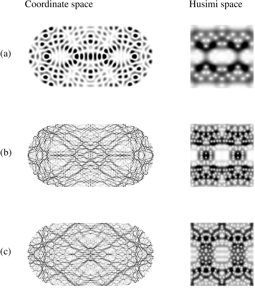
FIG. 1.: Representative eigenfunctions of the stadium billiard in coordinate space (left) with $x$-axis running from 0 to 4 and $y$-axis running from $-1$ to 1, and in Husimi phase space (right) with distance $q$ along the perimeter (horizontal axis) running clockwise from $0$ (corresponding to the center of the upper straight segment) to $4+2\pi$ and tangential momentum (vertical axis) running from $-k$ to $k$, where $k$ is the wavenumber of the eigenfunction. In the coordinate space plots, the graylevel represents $|\psi|^{2}$. In the Husimi phase space plots, white is high intensity and black low intensity. (a) $k=24.680$, (b) $k=100.787$ and (c) $k=105.608$, chosen to illustrate scarring along the bowtie and diamond orbits (cf. Table IV).

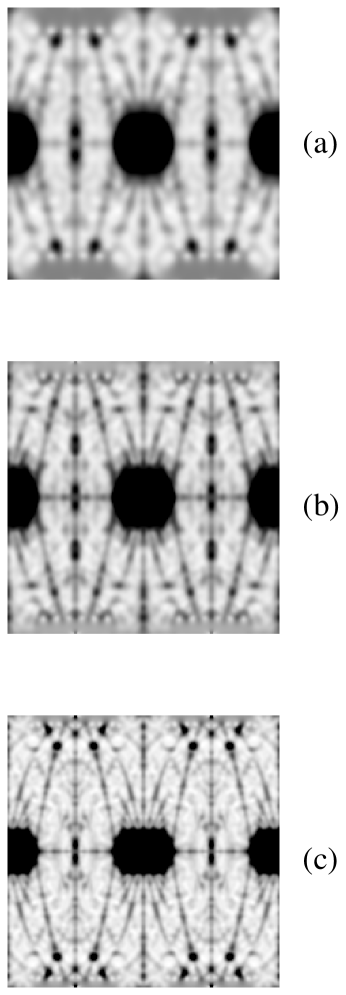
FIG. 2.: LIPR (see Eq. 7) in phase space as a function of $q$ running horizontally from $0$ to $4+2\pi$ and $p/k$ running vertically from $-1$ to $1$. The test-state width $\sigma$ is chosen so that the test Gaussians have circular cross-sections when the figures are plotted with a square aspect ratio. Darker shading indicates higher values. (a) $k=50$ to $60$, (b) $k=100$ to $150$, and (c) $k=200$ to $225$.

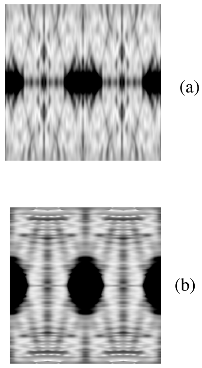
FIG. 3.: LIPR in phase space for eigenfunctions in the range from $k=100$ to $150$, coordinates as in Fig. 2(b), for (a) $\sigma^{2}\approx 0.01$, position-like test Gaussians, to be compared with $\sigma^{2}\approx 0.05$ used in Fig. 2(b), and (b) $\sigma^{2}\approx 0.25$, momentum-like test Gaussians.

FIG. 4.: Principal symmetry-related structures in phase space of the inverse-participation ratio plotted in Fig. 2 and the average-return probability plotted in Fig. 9. Schematic depiction of the symmetry lines in Fig. 2, labeled in the order in which they are described in the text.

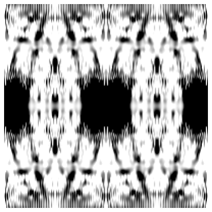
FIG. 5.: LIPR for real test wavepcakets (see Eq. (31)) in phase space as a function of $q$ running horizontally from $0$ to $4+2\pi$ and $p/k$ running vertically from $-1$ to $1$. The axes and parameters are the same as those used in Fig. 2.

(a)

(b)

FIG. 6.: Probability distribution of wavefunction intensities $I_{n}=\left|\mathinner{\mathchoice{\hbox{$\displaystyle\mathopen{\left<q,p\vphantom{n}\right|}\mathclose{\left.n\vphantom{q,p}\right>}$}}{\hbox{$\textstyle\mathopen{\left<q,p\vphantom{n}\right|}\mathclose{\left.n\vphantom{q,p}\right>}$}}{\hbox{$\scriptstyle\mathopen{\left<q,p\vphantom{n}\right|}\mathclose{\left.n\vphantom{q,p}\right>}$}}{\hbox{$\scriptscriptstyle\mathopen{\left<q,p\vphantom{n}\right|}\mathclose{\left.n\vphantom{q,p}\right>}$}}}\right|^{2}$ for the 1746 energy levels between $k=100$ and $150$. (a) For $(q,p)$ situated on the bowtie orbit. Solid line, numerical distribution of wavefunction intensities; dashed line, scar-corrected prediction of random-matrix theory with one degree of freedom; dotted line, random-matrix prediction, uncorrected for scarring. For purposes of illustration, the low-intensity part is shown in the figure on the left in a semilog plot and the high-intensity tail on the right in a log-log plot. (b) Same as (a) but for $(q,p)$ at a generic point in phase space, and the dashed line is now the random-matrix theory prediction for two degrees of freedom (without scar corrections, but adjusted for the 6% nearly vanishing intensities due to bouncing-ball states).

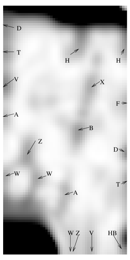
FIG. 7.: Principal dynamics-related structures in phase space of the inverse-participation ratio plotted in Fig. 2 and the average-return probability plotted in Fig. 9. The labeling is according to Table IV notation of scars on the principal short periodic orbits in Fig. 9(e), in an irreducible one-eighth region of phase space. The other regions of phase space are obtained by symmetry. The most prominent scarred orbits are W, Z, D, B, X and H.

FIG. 8.: Scatter plots of computed peak heights in columns 5 and 6 of Table III versus the linearized semiclassical predictions $S_{2}$ in column 4 and the brute-force semiclassical prediction in column 7. (a) Eigenfunctions ranging from $k=100$ to $150$, symmetry corrections included in $S_{2}$; (b) $k=200$ to $225$, symmetry corrections again included in $S_{2}$; (c) $k=100$ to $150$, but symmetry corrections not included in $S_{2}$. Without symmetry corrections the agreement is much worse. (d) $k=100$ to $150$ versus brute-force classical prediction without symmetry correction and (e) with symmetry corrections included.

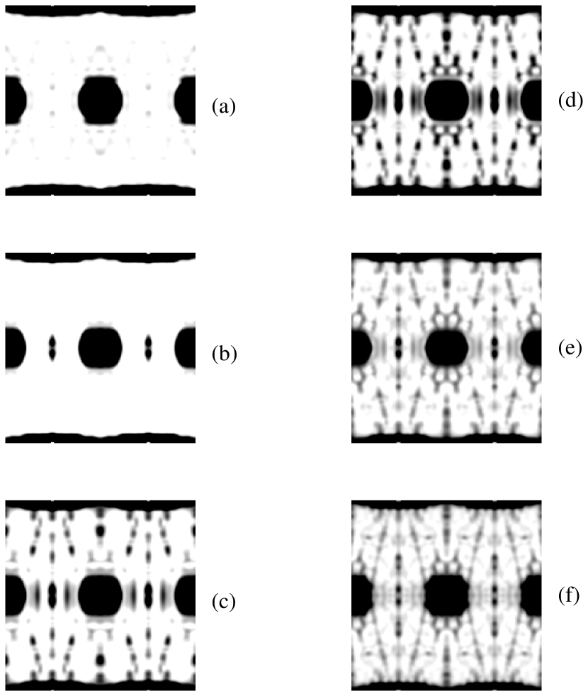
FIG. 9.: Quantum-mechanical average-return probability $P_{aa}(T)$ as defined in Eq. (77), near $k=100$; $q$ and $p$ as before. (a) $T=T_{B}$, (b) $T=2T_{B}$, (c) $T=3T_{B}$, (d) $T=4T_{B}$, (e) $T=5T_{B}$ and (f) $T=10T_{B}$. Note the emergence of periodic orbits at $T=2T_{B}$ to $T=3T_{B}$. For $T=10T_{B}$ the figure is already beginning to resemble the LIPR plotted in Fig. 2(b).

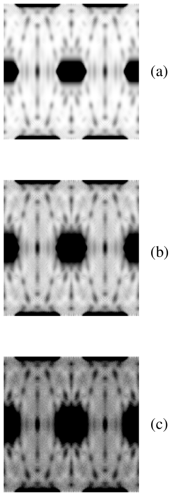
FIG. 10.: Results of a classical simulation of the return probability versus time, $q$ running horizontally from 0 to $4+2\pi$ and $p$ vertically from $-1$ to 1. Initial Gaussians were chosen with $\sigma^{2}=0.05$, corresponding to a spread in position space of 0.2 out of $4+2\pi$, or 2% of the perimeter. All of the major periodic orbits are present here as short-time recurrences. (a) $T=5T_{B}$, (b) $T=10T_{B}$, (c) $T=20T_{B}$.

REFERENCES

- [1] Electronic address: bies@fas.harvard.edu.
- [2] M. V. Berry, in Chaotic Behaviour of Deterministic Systems, ed. by G. Iooss, R. Helleman, and R. Stora (North-Holland 1983) p. 171.
- [3] E. J. Heller, Phys. Rev. Lett. 53, 1515 (1984).
- [4] S. W. McDonald, unpublished Ph.D. thesis, University of California at Berkeley.
- [5] L. Kaplan and E. J. Heller, Annals of Physics 264, 171 (1998); L. Kaplan, Phys. Rev. Lett. 80, 2582 (1998); see also the review: L. Kaplan, Nonlinearity 12, R1 (1999) and references therein.
- [6] L. Kaplan and E. J. Heller, Phys. Rev. E 59, 6609 (1999).
- [7] A. Bäcker, R. Schubert and P. Stifter, J. Phys. A 30, 6783 (1997); see also P.W. O’Connor and E.J. Heller, Phys. Rev. Lett. 61, 2288 (1989).
- [8] G. Tanner, J. Phys. A 30, 2863 (1997).
- [9] M. Sieber, U. Smilansky, S. C. Creagh and R. G. Littlejohn, J. Phys. A, 26, 6217 (1993); J. S. Espinoza Ortiz and A. M. Ozorio de Almeida, J. Phys. A 30, 7301 (1997).
- [10] A. Bäcker and R. Schubert, J. Phys. A 32, 4795 (1999); G. Casati and T. Prosen, Phys. Rev. E 59, R2516 (1999); B. Eckhardt, S. Fishman, J. Keating, O. Agam, J. Main and K. Muller, Phys. Rev. E 52, 5893 (1995).
- [11] E. J. Heller, Proc. Les Houches Summer School on ‘Chaos and Quantum Physics’ (Les Houches Session LII) ed. M. J. Giannoni, A. Voros and J. Zinn-Justin (Amsterdam: Elsevier, North-Holland, 1991), p. 602.
- [12] M. V. Berry, J. Phys. A 27, L391 (1994).
- [13] B. Li and B. Hu, J. Phys. A 31, 483 (1998); B. Li, Phys. Rev. E 55, 5376 (1997).
- [14] E. Vergini and M. Saraceno, Phys. Rev. E 52, 2204 (1995); F. P. Simonotti, E. Vergini and M. Saraceno, Phys. Rev. E 56, 3859 (1997).
- [15] P. A. Boasman, Nonlinearity 7, 485 (1994).
- [16] L. Kaplan and E. J. Heller, Physica D 121, 1 (1998).
- [17] E.J. Heller, J. Chem. Phys. 72, 1337-47 (1980); E.J. Heller, Phys. Rev. A 35, 1360 (1987).
- [18] E. B. Bogomolny, Nonlinearity 5, 805 (1992).
- [19] F. Mortessagne, O. Legrand, and D. Sornette, Chaos 3, 529 (1993).
- [20] P. W. O’Connor, S. Tomsovic and E. J. Heller, Physica D 55, 340 (1992).
(a)
(b)