Exact solutions and dynamics of globally coupled phase oscillators

Abstract

We analyze mean-field models of synchronization of phase oscillators with singular couplings and subject to external random forces. They are related to the Kuramoto-Sakaguchi model. Their probability densities satisfy local partial differential equations similar to the Porous Medium, Burgers and extended Burgers equations depending on the degree of singularity of the coupling. We show that Porous Medium oscillators (the most singularly coupled) do not synchronize and that (transient) synchronization is possible only at zero temperature for Burgers oscillators. The extended Burgers oscillators have a nonlocal coupling first introduced by Daido and they may synchronize at any temperature. Exact expressions for their synchronized phases and for Daido’s order function are given in terms of elliptic functions.

1 Introduction

Collective synchronization of large populations of nonlinearly coupled phase oscillators has been intensely studied since Winfree realized its importance for biological systems [1] and Kuramoto gave mathematical form to these ideas in a simple model [2, 3, 4]. Motivation for studying the Kuramoto model can be found in the broad variety of physical, chemical or biological phenomena which can be modelled within its framework (see [1, 5, 6, 7] and references therein).

The problem we want to consider is the dynamics of a system of nonlinearly, globally coupled phase oscillators with random frequencies $\omega_{i}$ [the probability for an oscillator to have frequency $\omega_{j}\in(\omega,\omega+d\omega)$ is $p(\omega)\,d\omega$], subject to external (independent, identically-distributed) white noise sources $\eta_{i}$ (of strength $\sqrt{2T}$):

$$\frac{\partial\phi_{i}}{\partial t}=\omega_{i}-\frac{K_{0}}{N}\sum_{j=1}^{N}f(\phi_{i}-\phi_{j})+\eta_{i}(t),$$ (1)

$i=1,\ldots,N$. Here $\phi_{i}(t)$ denotes the ith oscillator phase, $K>0$ represents the coupling strength, and $f$ is a generic real function of periodicity $2\pi$. In Fourier space, the latter can be decomposed as follows,

$$f(x)=\sum_{n=-\infty}^{\infty}a_{n}\exp(inx)$$ (2)

with $a_{n}=a_{-n}^{*}$.

Important work on the Kuramoto model with a general coupling function was carried out by Daido [8, 10] and Crawford [11] among others. Daido introduced the concept of order function to understand synchronization at zero temperature, $T=0$. Essentially, the order function is an average of the oscillator drift velocity on a rotating frame [9, 10]. Assuming a reasonable shape for the order function and the one-oscillator probability density (supposedly stationary in the rotating frame), Daido derived a functional equation for the order function. He then found solutions by direct numerical simulations and by bifurcation theory for stationary or rotating-wave probability densities. However, his theory is not sufficiently general to cover other possible probability densities (e.g., standing waves [15, 16]) nor to predict their stability properties. Crawford considered the problem of constructing one-oscillator probability densities which bifurcate from the incoherent density $1/(2\pi)$ (for which an oscillator has the same probability to be at any given value of the angle $\phi$) [11]. As a consequence of these works, different conjectures were proposed, both concerning scaling of bifurcating solution branches and general statements such as “adding noise could actually yield an enhancement in the level of synchronization” [11]. One difficulty with these previous works is that explicit calculations were performed mostly near bifurcation points. One exception is Daido’s coupling function $f(x)=$ sign$x$ for which the calculation of the order function can be explicitly carried out.

In this paper, we shall introduce classes of coupling functions leading to drift terms which are local functions of the probability density. We restrict ourselves to oscillators without frequency disorder, i.e., with frequency distribution $p(\omega)=$ $\delta(\omega)$. The corresponding governing equations for the probability density (in the limit of infinitely many oscillators) are systems of nonlinear partial differential equations which are analyzed. Then definite results can be proved about synchronization which do not depend on bifurcation calculations, order function theory or numerical simulations as much as the work of previous authors. Together with singular perturbation calculations, our results can be used to give approximations to the one-oscillator probability density of models with disorder, in the limiting case of high-frequencies [17]. The examples of singular coupling functions considered in this paper are the hard-needles (+ sign) and stick-needles (– sign) couplings, for which $f=\pm\delta^{\prime}$, the Burgers coupling, $f=\delta$, and the Daido coupling (extended Burgers model), $f(x)=$ sign$(x)$. In all cases, these $f$’s are extended periodically outside the interval $-\pi<x<\pi$. We shall show that less singular couplings give rise to models for which the oscillators are easier to synchronize: (i) the hard-needles oscillators do not synchronize at any temperature (the stick-needles coupling leads to ill-posed problems unless the temperature is large enough), (ii) the Burgers oscillators may synchronize only at zero temperature; even then, their probability density algebraically decays to incoherence as $t^{-1}$ for large times, (iii) the oscillators with Daido coupling may synchronize at any temperature, and the synchronized phases are described by explicitly-known order functions and probability densities. A first paper in the direction of these results was published by the authors in [12].

The rest of the paper is structured as follows. Section 2 contains results which hold for general models with disorder in the natural frequencies. These include a derivation of the governing equations for the one-oscillator probability density, its moments and the moment-generating function. We establish a relationship between these objects and Daido’s order function showing that the latter is proportional to the average oscillator drift in a rotating frame. Lastly, we give the leading-order form of the probability density in the limit of high frequencies. The density is a superposition of probability densities with zero natural frequency in rotating frames and with smaller coupling constants. In Section 3 we extend Daido’s approach to the case of nonzero temperature, and find the form of the stationary solutions and a general Liapunov functional for the case of odd coupling functions. In section 4 we introduce the family of singular couplings to be studied. Section 5 contains our analysis of the porous Medium models which appear for the hard-needles and stick-needles couplings. We show that the hard-needles model is well-posed, its solution exists globally, and also that sharp time decay estimates towards its equilibrium can be obtained locally for any initial data or globally for small initial data evolving exponentially fast towards incoherence. The last result is proven by different methods according to whether we allow the temperature to be zero. On the other hand, the stick-needles model is ill-posed for low enough temperature. Section 6 is devoted to study a model with Burgers coupling. We adapt well-known results to the case of periodic boundary conditions to show that the probability density of the Burgers oscillators may tend to a state different from incoherence only if the temperature is zero. In section 7 we analyze the extended Burgers model resulting from the Daido coupling $f(x)=$ sign$(x)$. We first show that finding the probability density is equivalent to solving two coupled nonlinear parabolic equations for the drift $v(x,t)$ and a certain functional of the probability density, $\sigma(x,t)$. Then we find families of stationary solutions in terms of elliptic functions. These solutions bifurcate supercritically from incoherence at couplings $K_{0}$ which are proportional to the squares of odd integer numbers, and stationary densities on the first bifurcating branch are stable at least for small enough $K_{0}$. We discuss some of the results of previous authors in the light of our exact calculations. The Appendices discuss technical matters related to the bulk of the article.

2 Probability density and moment-generating function

In this section we consider general aspects of the model (1). First of all, we use the moment approach considered in [13] to derive a nonlinear Fokker-Planck equation (NLFPE) for the one-oscillator probability density in the limit of infinitely many oscillators. The moment approach exploits the symmetry of the dynamical problem we are interested in, so is a good starting point to deal with the Kuramoto model which has rotational symmetry (an extension of this method to deal with tops has been considered in [14]). Secondly, we characterize phase and frequency synchronization generalizing to $T\neq 0$ the concept of order function introduced by Daido [8] for oscillator synchronization at $T=0$. Lastly, we show that, at high frequencies, the probability density can be decomposed into $m$ components rotating steadily at the frequencies of the peaks of a given multimodal natural frequency distribution. Each component probability density solves a NLFPE with zero natural frequency (in the rotating frame) and a modified coupling constant. This latter results follows immediately from the method introduced in Ref. [17] for the usual Kuramoto model with a sinusoidal coupling function. This result can be combined with the exact solutions obtained in later Sections to yield analytic expressions of synchronized phases in models with frequency disorder and white noise forcing in the high-frequency limit.

2.1 Nonlinear Fokker-Planck equation

To start with let us define,

$$H_{k}^{m}=\frac{1}{N}\sum_{j=1}^{N}\,\overline{\langle\exp(ik\phi_{j})\rangle\omega_{j}^{m}}\,,$$ (3)

where the brackets denote average with respect to the external noise and the overbar average with respect to the random oscillator frequency. This set of moments is invariant under the local symmetry $\phi_{i}\to\phi_{i}+2\pi$ which is the symmetry of the dynamical equations 1. The equation of motion for the moments reads

$$\frac{\partial H_{k}^{m}}{\partial t}=-K_{0}ik\sum_{n=-\infty}^{\infty}a_{n}H_{k+n}^{m}H_{-n}^{0}-k^{2}TH_{k}^{m}\,+\,ikH_{k}^{m+1}.$$ (4)

It is easy to derive from Eq.(4) the following differential equation

$$\frac{\partial g}{\partial t}=-\frac{\partial}{\partial x}\Bigl{[}v(x,t)\,g\Bigr{]}+T\frac{\partial^{2}g}{\partial x^{2}}-\frac{\partial^{2}g}{\partial x\partial y}\,$$ (5)

for the generating function

$$g(x,y,t)={1\over 2\pi}\,\sum_{k=-\infty}^{\infty}\sum_{m=0}^{\infty}\exp(-ikx)\frac{y^{m}}{m!}H_{k}^{m}(t).$$ (6)

The velocity $v(x,t)$ is defined by

$$v(x,t)=-K_{0}\sum_{n=-\infty}^{\infty}a_{n}H_{-n}^{0}\exp(inx)$$ (7)

and it can be equivalently written as a convolution between the coupling and the generating function (see A):

$$v(x,t)\ =\ -K_{0}\,\int_{-\pi}^{\pi}f(x^{\prime})g(x-x^{\prime},0,t)\ dx^{\prime}.$$ (8)

Notice that this drift velocity is related to Daido’s order function $H(x,t)$ [9] (see B):

$$v(x,t)=-K_{0}\,H(x-\Omega_{e}t,t).$$ (9)

The case analyzed by Kuramoto corresponds to the force $f(x)=\sin x$. Then $a_{1}=a_{-1}^{*}=-i/2$ and the rest of components are zero. This yields $v(x,t)=K_{0}r\sin(\theta-x)$, where $H_{1}^{0}=r\exp(i\theta)$. Let us assume that there exists a probability density $\rho(x,\omega,t)$ such that

$${1\over N}\sum_{j=1}^{N}{\cal F}(\phi_{j}(t),\omega_{j})=\int_{-\pi}^{\pi}\int_{-\infty}^{\infty}{\cal F}(x,\omega)\,\rho(x,\omega,t)\,p(\omega)\,d\omega\,dx,$$ (10)

as $N\to\infty$. In particular, we assume that

$$\rho(x,\omega,t)\,p(\omega)={1\over N}\sum_{j=1}^{N}\delta(x-\phi_{j}(t))\,\delta(\omega-\omega_{j})\,,$$ (11)

tends to a smooth function in the limit as $N\to\infty$. We can relate the probability density to the moment-generating function as follows:

$$g(x,y,t)={1\over 2\pi}\sum_{k=-\infty}^{\infty}\sum_{m=0}^{\infty}e^{-ikx}{y^{m}\over m!}{1\over N}\sum_{j=1}^{N}e^{ik\phi_{j}(t)}\omega_{j}^{m}$$

$$={1\over N}\sum_{j=1}^{N}e^{y\omega_{j}}{1\over 2\pi}\sum_{k=-\infty}^{\infty}e^{ik[\phi_{j}(t)-x]}={1\over N}\sum_{j=1}^{N}e^{y\omega_{j}}\delta(\phi_{j}(t)-x)$$

$$=\int_{-\infty}^{\infty}e^{y\omega}\,\rho(x,\omega,t)\,p(\omega)\,d\omega.$$ (12)

Then the probability density can be written as follows

$$\rho(x,\omega,t)\,p(\omega)={1\over 2\pi}\int_{-\infty}^{\infty}g(x,iy,t)\,e^{-i\omega y}\,dy$$ (13)

and

$$-{1\over 2\pi i}\int_{-\infty}^{\infty}e^{-i\omega y}{\partial g\over\partial y}\,dy=-\omega\,\rho(x,\omega,t)\,p(\omega).$$ (14)

By using these expressions in (5), we derive the usual nonlinear Fokker-Planck equation (NLFPE) for $\rho(x,\omega,t)$ wherever $p(\omega)\neq 0$:

$$\frac{\partial\rho}{\partial t}+\frac{\partial}{\partial x}\Bigl{[}(\omega+v)\,\rho\Bigr{]}=T\frac{\partial^{2}\rho}{\partial x^{2}}\,.$$ (15)

Equations (10) and (8) provide us with the following formula for the drift velocity $v$ in terms of $\rho$:

$$v(x,t)\ =\ -K_{0}\int_{-\pi}^{\pi}\int_{-\infty}^{\infty}f(x^{\prime})\rho(x-x^{\prime},\omega,t)p(\omega)\,dx^{\prime}d\omega.$$ (16)

The probability density $\rho$ should moreover satisfy a normalization condition $\int_{-\pi}^{\pi}\rho dx=1$ and an initial condition $\rho(x,\omega,0)=\rho_{0}(x,\omega)$. A derivation of these problems by path integral methods can be found in [18]. (The path integral derivation is applicable to each Fourier mode of the coupling function; see page 676 of [18]). See [19, 20] for rigorous proofs of (10), (15) - (16) in different models.

2.2 Phase and frequency distributions

To characterize oscillator synchronization, it is convenient to define the phase and frequency probability densities. The phase probability density, $P(\phi,t)$, is the probability of finding an oscillator with angle in $(\phi,\phi+d\phi)$ independently of its frequency. It is given by

$$P(\phi,t)=\int_{-\pi}^{\pi}\int_{-\infty}^{\infty}\delta(x-\phi)\,\rho(x,\omega,t)\,p(\omega)\,dx\,d\omega.$$ (17)

Similarly, we may define the frequency of a given oscillator as the average (when it exists)

$${1\over\tau}\,\int_{0}^{\tau}{d\phi_{j}\over dt}\,dt,$$

for sufficiently large $\tau>0$. When $N\to\infty$, (1) and the ergodic theorem imply that the previous time average is equal to

$$\omega+{1\over\tau}\,\int_{0}^{\tau}v(x,t)\,dt,$$

where $\omega=\omega_{j}$. Then we may define the frequency density as

$$P(\omega,t)=\int_{-\pi}^{\pi}\int_{-\infty}^{\infty}\delta\left(\Omega-\omega-{1\over\tau}\,\int_{0}^{\tau}v(x,t^{\prime})\,dt^{\prime}\right)\rho(x,\Omega,t)\,p(\omega)\,dx\,d\Omega$$ (18)

that can be simplified in the important cases of: stationary (i) and rotating-wave (ii) probability densities. In case (i), $v=v(x)$ coincides with its time average, and is proportional to Daido’s order function with $\Omega_{e}=0$. In case (ii), $\rho(x,\Omega,t)=\tilde{\rho}(x-\Omega_{e}t,\Delta)$, with $\Delta=\Omega-\Omega_{e}$ and, according (9), $v(x,t)=-K_{0}\,H(x-\Omega_{e}t)$. Then the change of variable $\psi=x-\Omega_{e}t$ reduces probability density and order function to time-independent functions so that (18) becomes

$$P(\omega)=\int_{-\pi}^{\pi}\int_{-\infty}^{\infty}\delta[\omega-\Omega_{e}-\Delta+K_{0}\,H(\psi)]\,\tilde{\rho}(\psi,\Delta)\,\tilde{p}(\Delta)\,d\psi\,d\Delta,$$ (19)

where $\tilde{p}(\Delta)=p(\Omega_{e}+\Delta)$. Daido considered only cases (i) and (ii) at $T=0$ with an order function having a single minimum $H_{min}$ (resp. maximum $H_{max}$) at $\psi=\psi_{1}$ (resp. $\psi=\psi_{2}$) [8]. Then the probability density is

$$\tilde{\rho}(\psi,\Delta)=\delta\left(\psi-H^{-1}\left({\Delta\over K_{0}}\right)\right)\,\chi_{(\psi_{1},\psi_{2})}(\psi)$$

$$+{C(\Delta)\over\Delta-K_{0}\,H(\psi)}\,\left[1-\chi_{(\psi_{1},\psi_{2})}(\psi)\right]\,,$$ (20)

where

$$C(\Delta)={2\pi\over\int_{-\pi}^{\pi}{d\psi\over\Delta-K_{0}H(\psi)}}\,,$$ (21)

$\psi=\phi-\Omega_{e}t$, with $\Delta$ as before and $\chi_{(\psi_{1},\psi_{2})}(\psi)$ equals 1 if $\psi_{1}<\psi<\psi_{2}$ and 0 otherwise. On the interval $-\pi<\psi<\pi$ the order function $H(\psi)$ is stationary as before. $C(\Delta)$ is the frequency at which oscillators with angle outside $(\psi_{1},\psi_{2})$ rotate. Inside $(\psi_{1},\psi_{2})$ we have $K_{0}H(\psi)=\Delta$ and $d\psi/dt=0$. Inserting (20) in (16) and (9) we find a functional equation for the order function, which can then be solved exactly or approximately [8]. Daido’s expressions for the angle and frequency densities are found by inserting (20) in (17) and (19) (minor notational changes have been made) [8]

$$P(\psi)=K_{0}\,\tilde{p}(K_{0}H(\psi))\,H^{\prime}(\psi)\,\chi_{(\psi_{1},\psi_{2})}(\psi)+\left[1-\chi_{(\psi_{1},\psi_{2})}(\psi)\right]\,$$

$$\times\int_{-\infty}^{\infty}{C(\Delta)\tilde{p}(\Delta)\over\Delta-K_{0}\,H(\psi)}\,\chi_{(-\infty,K_{0}H_{min})}(\Delta)\,\chi_{(K_{0}H_{max},\infty)}(\Delta)\,d\Delta,$$ (22)

$$P(\omega)=\delta(\omega-\Omega_{e})\,\int_{K_{0}H_{min}}^{K_{0}H_{max}}\tilde{p}(\Delta)d\Delta+{\tilde{p}(C^{-1}(\omega-\Omega_{e}))\over C^{\prime}(C^{-1}(\omega-\Omega_{e}))}\,.$$ (23)

2.3 High-frequency limit

Further general considerations can be made for multimodal natural frequency distributions in the limit of high frequencies [17]. Let us assume that $p(\omega)$ has $m$ maxima located at $\omega_{0}\Omega_{l}$, $l=1,\ldots,m$, where $\omega_{0}\rightarrow\infty$, and $p(\omega)\,d\omega$ tends to the limit distribution

$$\Gamma(\Omega)\,d\Omega\equiv\sum_{l=1}^{m}\alpha_{l}\,\delta(\Omega-\Omega_{l})\,d\Omega,$$ (24)

$$\mbox{with}\quad\quad\sum_{l=1}^{m}\alpha_{l}=1,\quad\mbox{and}\quad\Omega=\frac{\omega}{\omega_{0}}\,,$$

independently of the shape of $p(\omega)$ as $\omega_{0}\to\infty$. $p(\omega)\,d\omega$ and $\Gamma(\Omega)\,d\Omega$ may be used interchangeably when calculating any moment of the probability density [including of course the all-important velocity function (16), which is related to Daido’s order function as said before]. Thus any frequency distribution is equivalent to a discrete multimodal distribution in the high-frequency limit. The discrete symmetric bimodal distribution considered in [21, 22] corresponds to $m=2$, $\Omega_{l}=(-1)^{l}$, $\alpha_{l}={1\over 2}$, $l=1,2$. By following the procedure explained in [17], we can show that the oscillator probability density splits into $m$ components, each contributing a wave rotating with frequency $\Omega_{l}\omega_{0}$ to the order function:

$$\rho(x,\omega,t)=\sum_{l=1}^{m}\rho_{l}^{(0)}(x-\Omega_{l}\omega_{0}t,t)+O(\omega_{0}^{-1}).$$ (25)

The densities $\rho_{l}^{(0)}$ obey the following Fokker-Planck equation

$${\partial\rho_{l}^{(0)}\over\partial t}-T{\partial^{2}\rho_{l}^{(0)}\over\partial\beta^{2}}-K_{0}\alpha_{l}\,\frac{\partial}{\partial\beta}\left\{\rho_{l}^{(0)}\,\int_{-\pi}^{\pi}f(\beta-\beta^{\prime})\rho_{l}^{(0)}(\beta^{\prime},t)d\beta^{\prime}\right\}=0,$$ (26)

where $\beta=x-\Omega_{l}\omega_{0}t$ and each $\int_{-\pi}^{\pi}\rho_{l}^{(0)}d\beta=1$. This equation corresponds to the NLFPE (15) - (16) in the moving variable $\beta$, with a coupling constant $K_{0}\alpha_{l}$ instead of $K_{0}$ and $p(\omega)=\delta(\omega)$. We shall see below that its solution evolves to a stationary state as the time elapses provided $f(x)$ is odd. Thus the probability density (to leading order in $1/\omega_{0}$) is the sum of $m$ components obeying the stationary solution of (26) with variables $x-\Omega_{l}\omega_{0}t$. The overall velocity (related to the order function) is a superposition of $m$ waves each traveling with frequency $\Omega_{l}\omega_{0}$

$$v(x,t)=-K_{0}\,\sum_{l=1}^{m}\alpha_{l}\,\int_{-\pi}^{\pi}f(x-\Omega_{l}\omega_{0}t-\beta^{\prime})\rho_{l}^{(0)}(\beta^{\prime})d\beta^{\prime}\,,$$ (27)

where $\rho_{l}^{(0)}(x)$ is the stationary solution of (26).

We shall now consider NLFPE without disorder, i.e., $\omega_{i}=0$ or $p(\omega)=\delta(\omega)$. Our results will be applicable to models with a multimodal natural frequency distribution in the high-frequency limit. For a model without disorder, the moment-generating function is independent of $y$ and it equals the probability density: $g(x,y,t)=\rho(x,0,t)\equiv g(x,t)$. If detailed balance is obeyed (i.e. if $f$ is an odd function) then the model is purely relaxational and consequently the formalism of statistical mechanics can be applied.

3 Stationary solutions of models with odd coupling

We can find functional equations for the order function of stationary or rotating wave solutions at nonzero temperatures without making Daido’s assumptions. In this section we shall assume detailed balance, which occurs when $f$ is an odd function extended periodically outside $(-\pi,\pi)$ and satisfying $f(x+\pi)=-f(x)$. (The expressions for the general case are somewhat more complicated). Let us define

$$V(x,t)=\int_{-\pi}^{x}v(s,t)\,ds,$$ (28)

$$W(x,\omega,t)=(\pi+x)\omega+V(x,t).$$ (29)

The property $f(x+\pi)=-f(x)$ implies that the drift (16) satisfies $v(x+\pi,t)=-v(x,t)$, and $V(x+\pi,t)=V(0,t)-V(x,t)$.

3.1 Stationary solutions

Let us restrict ourselves to the case of stationary solutions; rotating wave solutions may be reduced to this case after moving to a rotating frame. The stationary solutions should have the form

$$\rho(x,\omega) = Z^{-1}\,e^{{W(x,\omega)\over T}}$$ (30)

$$- {J\over T}\int_{-\pi}^{x}\exp\left[{W(x,\omega)-W(s,\omega)\over T}\right]\,ds,$$

where $Z$ and $J$ are functions of $\omega$, independent of $x$. We now impose the condition that $\rho$ be a $2\pi$-periodic function of $x$, use the symmetry properties of the drift, and find the probability flux $J$ as a function of $Z$:

$${J\over T}={2\,\mbox{sinh}\left({2\pi\omega\over T}\right)\over Z\int_{-\pi}^{\pi}e^{-{W(x,\omega)\over T}}\,dx}\,.$$ (31)

$Z$ can be found from the normalization condition $\int_{-\pi}^{\pi}\rho dx=1$. The functional equation for the drift $v(x)$ (or, equivalently, the order function) is obtained by inserting (30), (31) and the formula for $Z$ in (16). The result is

$${v(x)\over K_{0}}=\int_{-\pi}^{\pi}f(x-x^{\prime})\int_{-\infty}^{\infty}{e^{{W(x^{\prime},\omega)\over T}}\over Z(\omega)}\left\{2\mbox{sinh}\left({2\pi\omega\over T}\right)\right.$$

$$\left.\times\,{\int_{-\pi}^{x^{\prime}}e^{-{W(s,\omega)\over T}}\,ds\over\int_{-\pi}^{\pi}e^{-{W(s,\omega)\over T}}\,ds}-1\right\}\,p(\omega)\,d\omega\,dx^{\prime},$$ (32)

$$Z(\omega) = \int_{-\pi}^{\pi}e^{{W(x,\omega)\over T}}\left\{{2\mbox{sinh}\left({2\pi\omega\over T}\right)\int_{-\pi}^{x}e^{-{W(s,\omega)\over T}}ds\over\int_{-\pi}^{\pi}e^{-{W(s,\omega)\over T}}\,ds}-1\right\}\,dx.$$

The functional equation (32) for $v(x)$ may in general have several solutions, depending on $p(\omega)$ and the value of the parameters $K_{0}$ and $T$. Notice that no assumption on the shape of the order function has been made in order to derive (32). Thus we have a general equation for $v(x)$ valid for any temperature thereby extending Daido’s theory. If $f(x)$ is not odd, the same procedure yields a more cumbersome equation which we omit. An interesting case corresponds to the case without disorder, $p(\omega)=\delta(\omega)$, for which $J=0$, $\rho(x,0,t)=g(x,y,t)\equiv g(x,t)$, and

$$g_{0}(x)={e^{{V_{0}(x)\over T}}\over\int_{-\pi}^{\pi}e^{{V_{0}(s)\over T}}\,ds}\,.$$ (33)

The subscript zero just reminds us that we are considering stationary solutions. In this case there is a general Liapunov functional related to the free energy [23]. In Sections 4, 5 and 6, we show that simpler quadratic Liapunov functionals may exist for specific forms of $f(x)$.

3.2 Liapunov functional

Let us define the relative entropy

$$\eta(t)=\int_{-\pi}^{\pi}g(x,t)\,\ln\left({g(x,t)\over\overline{g}(x,t)}\right)\,dx,$$ (34)

$$\overline{g}(x,t)=e^{{V(x,t)-\mu(t)\over T}}\,,$$ (35)

$${d\mu\over dt}=\int_{-\pi}^{\pi}g(x,t)\,{\partial V(x,t)\over\partial t}\,dx.$$ (36)

$V(x,t)$ is given by (28) with the drift calculated by means of the exact probability density $g(x,t)$. (36) implies that

$$\int_{-\pi}^{\pi}g(x,t)\,{\partial\over\partial t}\ln\overline{g}(x,t)\,dx=0.$$

Direct calculation shows that

$${d\eta\over dt}=-T\int_{-\pi}^{\pi}g(x,t)\,\left|{\partial\over\partial x}\ln\left({g(x,t)\over\overline{g}(x,t)}\right)\right|^{2}\,dx\leq 0.$$ (37)

The inequality $y\ln y\geq y-1$, $\forall y\geq 0$, can be used to show that

$$\eta\geq 1-\int_{-\pi}^{\pi}\overline{g}(x,t)\,dx.$$ (38)

Then the relative entropy is bounded below if $e^{V(x,t)}\in\mbox{L}^{1}(-\pi,\pi)$ and the function $\mu(t)$ is bounded below. The first condition thanks to the Trudinger-Moser theorem (see [24]) is always fulfilled if $V(x,t)$ is in the Sobolev space $W^{1,1}_{0}(-\pi,\pi)$ and this property is verified for $V(x,t)$ defined in (28). To show that the function $\mu(t)$ is bounded below let us write Eq. (36) as follows

$${d\over dt}\left[\mu-\int_{-\pi}^{\pi}g\,V\,dx\right]=-\int_{-\pi}^{\pi}V\,{\partial g\over\partial t}\,dx$$

$$=-\int_{-\pi}^{\pi}v\,\left[vg-T{\partial g\over\partial x}\right]\,dx=-\int_{-\pi}^{\pi}v(x,t)\,J(x,t)\,dx,$$ (39)

after using the nonlinear Fokker-Planck equation and integration by parts. $J$ $\equiv vg$ $-T\,\partial g/\partial x$ is the probability flux. Then (39) can be equivalently written as

$$\mu(t)=\int_{-\pi}^{\pi}\left[g(x,t)\,V(x,t)\,-g(x,0)\,V(x,0)\right]dx$$

$$-\int_{0}^{t}\int_{-\pi}^{\pi}v(x,s)\,J(x,s)\,dx\ ds.$$ (40)

Let us first note that, since $\int_{-\pi}^{\pi}g\,dx=1$ and $V$ is a uniformly bounded function, the two first terms in the right hand side of (40) are bounded. If we can prove that

$$\int_{0}^{t}\int_{-\pi}^{\pi}v(x,s)\,J(x,s)\,dx\ ds$$

is uniformly bounded, then $\mu(t)$ will remain bounded for all time and the demonstration that $\eta$ is a Liapunov functional will be over. By using the symmetry of $f(x)$ and the definitions of $J$ and $v$, it is easy to show first that

$$\int_{-\pi}^{\pi}J(x,t)\,dx=0,\quad\forall t.$$

Since $J$ is a continuous function with respect to $x$, the mean value theorem applied to the above equality implies the existence of $a_{t}\in[-\pi,\pi]$ such that $J(a_{t},t)=0$, where the subscript makes reference to the fixed time $t$ and $a_{t}$ is chosen so that the function $J$ has a definite sign over $(a_{t},x)$. Then

$$\int_{0}^{t}\int_{a_{t}}^{x}v(x,s)\,J(x,s)\,dx\ ds\leq\mbox{max}_{x,t}|v(x,t)|\,\int_{a_{0}}^{x}\left[\mbox{sign}J(x,t)\,\int_{0}^{b_{x}}J(x,s)ds\right]\,dx,$$

where $t=b_{x}$ is the inverse function of $x=a_{t}$. Now we integrate

$${\partial g\over\partial t}=-T{\partial J\over\partial x}$$

over $(a_{0},x)\times(0,b_{x})$, and obtain

$$\int_{a_{t}}^{x}[g(y,t)-g(y,0)]\,dy=-T\,\int_{0}^{t}\int_{a_{t}}^{x}{\partial J(y,s)\over\partial y}\,dyds=-T\,\int_{0}^{t}J(x,s)ds,$$

where we have used again Fubini’s theorem to exchange the order of integration in the right hand side. The left hand side of this equation is bounded by 2, so that we obtain after taking the limit as $t\to\infty$,

$$\lim_{t\to\infty}\int_{0}^{t}J(x,s)\,ds\ \leq\ {1\over T}\lim_{t\to\infty}\int_{a_{t}}^{x}[g(y,t)-g(y,0)]\,dy\ \leq\ {2\over T}.$$

Combining this bound with the uniform one for $v(x,t)$ and taking into account that

$$\int_{0}^{t}\int_{-\pi}^{\pi}v(x,s)\,J(x,s)\,dx\,ds\,=\,\sum_{j\in\Lambda}\int_{0}^{t}\int_{a_{t}^{j}}^{x}v(x,s)\,J(x,s)\,dx\,ds,$$

where $\Lambda$ is a finite set of indices because of $J\in C^{1}$ has a finite number of zeros in $[-\pi,\pi]$, we deduce that the third term in (40) is also uniformly bounded and, as consequence, $\mu(t)$ is bounded from below.

Our Liapunov functional may be used to show that $g(x,t)$ tends to a stationary solution as time elapses and also to discuss the global stability of these solutions. Let $g_{\infty}(x,t)$ be the limiting probability density as $t\to\infty$. Equating the entropy production (37) to zero, we obtain $g_{\infty}=\beta(t)$ exp$V(x,t)/T$. Inserting this into (15), we find

$${d\beta\over dt}+{\beta\over T}\,{\partial V(x,t)\over\partial t}=0,$$

which may be rewritten as

$${T\over\beta}{d\beta\over dt}=-{\partial V(x,t)\over\partial t}\,.$$

The left side of this expression is independent of $x$ whereas the second side is not, so that both sides are zero. Then $V$ is time independent and $\beta$ is a constant, which proves $g_{\infty}$ to be of the form (33).

3.3 Equilibrium states

The previous considerations suggest that for models with odd-coupling functions and no frequencies [i.e. $f(-x)=-f(x)$ and $p(\omega)=\delta(\omega)$], a thermodynamic formulation will suffice to identify the stationary states as well as the possible existence of thermodynamic singularities (i.e., bifurcations).

In order to demonstrate this assertion, we shall start by defining an appropriate energy function,

$${\cal H}=\frac{K_{0}}{N}\,\sum_{i<j}E(\phi_{i}-\phi_{j})$$ (41)

where $E(x)$ is a two-pair interaction energy function defined by $E(x)=\int_{-\pi}^{x}f(s)ds$ and $E(x)=E(x+2\pi)$. The $2\pi$-periodicity of $E(x)$ is crucial to derive the results of this section. Note that this newly introduced function is related to the potential $V(x,t)$ in Eq. (28) by

$$-{V(x,t)\over K_{0}}=\int_{-\infty}^{\infty}\int_{-\pi}^{\pi}E(x-x^{\prime})\rho(x^{\prime},\omega,t)p(\omega)dx^{\prime}d\omega$$

$$-\int_{-\infty}^{\infty}\int_{-\pi}^{\pi}E(-\pi-x^{\prime})\rho(x^{\prime},\omega,t)p(\omega)dx^{\prime}d\omega.$$ (42)

which has the physical meaning of an averaged energy. The second term is an additive constant which fixes the origin of the energy scale. Consequently the Liapunov functional defined in Eq. (34) is a generalized free energy for the system. Now we want to show that the equilibrium state of such a system yields potential solutions identical to (33). Let us compute the partition function,

$${\cal Z}=\int_{-\pi}^{\pi}\ldots\int_{-\pi}^{\pi}e^{-\beta{\cal H}}\,\prod_{i=1}^{N}d\phi_{i}\quad\quad\quad\quad\quad\quad\quad\quad\quad$$

$$=\int_{-\pi}^{\pi}\ldots\int_{-\pi}^{\pi}\exp\left(-\frac{\beta K_{0}}{N}\sum_{i<j}E(\phi_{i}-\phi_{j})\right)\,\prod_{l=1}^{N}d\phi_{l}.$$ (43)

We have $a_{0}=0$ because $f$ is odd. Then we can write $E(x)=\sum_{n=-\infty}^{\infty}b_{n}e^{inx}$ (plus an unessential constant term), where $b_{0}=0$, $b_{n}=-i(a_{n}/n)\,(n\neq 0)$. Consequently we can rewrite the partition function for an oscillator system without frequency disorder, $p(\omega)=\delta(\omega)$, as

$${\cal Z}=\int_{-\pi}^{\pi}\ldots\int_{-\pi}^{\pi}\exp\left\{-\frac{\beta K_{0}}{2N}\sum_{n=-\infty}^{\infty}\left(\sum_{i=1}^{N}e^{in\phi_{i}}\sum_{j=1}^{N}e^{-in\phi_{j}}\right)\right\}\,\prod_{l=1}^{N}d\phi_{l}.$$ (44)

We have neglected the contribution of the terms $(i=j)$ in the exponential (which is equivalent to redefine the origin of energies so that $E(0)=0$). Let us now insert delta functions in the previous integrals and use the identity,

$$1 = \int_{-\infty}^{\infty}\delta\left(h_{n}-\frac{1}{N}\sum_{i=1}^{N}e^{in\phi_{i}}\right)\,dh_{n}$$

$$= \int_{-\infty}^{\infty}\int_{-\infty}^{\infty}\exp\left\{i\lambda_{n}\left(h_{n}-\frac{1}{N}\sum_{i=1}^{N}e^{in\phi_{i}}\right)\right\}\,dh_{n}d\lambda_{n},$$

where the new set of Lagrange multipliers $\lambda_{n}$ has been introduced. Inserting these representations of the delta function in (44) and permuting the orders of the integration between the $\phi^{\prime}s$ and the $h_{n},\lambda_{n}$, we reduce the final expression to a single site problem,

$${\cal Z}=\int_{-\infty}^{\infty}\exp[NA(\lambda,h)]\,\prod_{n=-\infty}^{\infty}d\lambda_{n}dh_{n},$$ (45)

where

$$A(\lambda,h)=-\sum_{n=-\infty}^{\infty}\lambda_{n}h_{n}-\frac{\beta K_{0}}{2}\sum_{n=-\infty}^{\infty}b_{n}h_{n}h_{-n}$$

$$+\log\int_{-\pi}^{\pi}\exp\left(\sum_{n=-\infty}^{\infty}\lambda_{n}e^{in\phi}\right)\,d\phi.$$ (46)

The dominant contribution to the partition function is determined by the saddle point equations,

$$\frac{\partial A}{\partial\lambda_{n}}=\frac{\partial A}{\partial h_{n}}=0$$ (47)

which yield,

$$h_{n} = <\exp(in\phi)>,$$ (48)

$$\lambda_{n} = -\frac{\beta K_{0}}{2}h_{-n}(b_{n}+b_{-n})=-\beta K_{0}h_{-n}\,\mbox{Re}(b_{n})\,.$$ (49)

Here the average $<B(\phi)>$ of an arbitrary function $B(\phi)$ is defined as follows

$$<B(\phi)>=\frac{\int_{-\pi}^{\pi}B(\phi)\,\exp\bigl{(}\sum_{n=-\infty}^{\infty}\lambda_{n}e^{in\phi}\bigr{)}\,d\phi}{\int_{-\pi}^{\pi}\exp\bigl{(}\sum_{n=-\infty}^{\infty}\lambda_{n}e^{in\phi}\bigr{)}\,d\phi}.$$ (50)

The next steps are quite standard. Inserting the expression (49) for $\lambda_{n}$ into (48), we obtain a closed set of equations for the parameters $h_{n}$. The reader will easily convince himself that the parameters $h_{n}$ are nothing less that the moments defined in Eq. (3) (with $\omega_{i}=0$). Finally we find that the effective Hamiltonian in the exponent of (50) is exactly given by the potential function $V_{0}(x)$ of eq.(28). Then the equilibrium density function $g(x)$ should satisfy

$$g(x)=<\delta(x-\phi)>=\frac{\exp(\beta\tilde{V}(x))}{\int_{-\pi}^{\pi}\exp(\beta\tilde{V}(x))\,dx}\,,$$ (51)

with

$$\tilde{V}(x)=-K_{0}\sum_{n=-\infty}^{\infty}(Reb_{n})h_{-n}\exp(inx)dx.$$ (52)

This coincides with the definition (28) [$\tilde{V}(x)=V(x)+$constant] if all the $b_{n}$ are real i.e. if $f(x)$ is an odd function. From (48) and (49) it follows that the function $v(x)$ is a solution of the following functional equation

$$v(x)=-K_{0}<f(x-\phi)>=-K_{0}\frac{\int_{-\pi}^{\pi}f(x-\phi)\,e^{\beta V(\phi)}d\phi}{\int_{-\pi}^{\pi}e^{\beta V(\phi)}\,d\phi}.$$ (53)

The system of equations (28) and (53) may have one, many or no solutions. In case of multiple solutions, the free energy and the dynamics should be used to fully characterize the equilibrium state.

4 A family of models

When $p(\omega)=\delta(\omega)$, Eq.(5) becomes

$$\frac{\partial g}{\partial t}=-\frac{\partial}{\partial x}\Bigl{[}v(x,t)g\Bigr{]}+T\frac{\partial^{2}g}{\partial x^{2}}\,.$$ (54)

The probability density $g(x,t)$ obeys the natural normalization condition

$$\int_{-\pi}^{\pi}g(x,t)\,dx=1\,.$$ (55)

Let us consider the following special cases of localized coupling functions $f$:

• (a) The hard-needles model: In this case $f=\delta^{\prime}$ and (5) and (8) yield

  $$\frac{\partial g}{\partial t}=K_{0}\frac{\partial}{\partial x}\Bigl{(}g\frac{\partial g}{\partial x}\Bigr{)}+T\frac{\partial^{2}g}{\partial x^{2}}\,.$$ (56)

  Note that in this case there is an energy of the model given by $E=\sum_{i<j}\delta(\phi_{i}-\phi_{j})$ which is trivially zero except when two phases coincide. If we imagine the phases as needles located in the centre of the unit circle then the crossing of needles costs infinite energy. This is the reason for its name: In this case the needles are impenetrable and interact like the hard spheres in the theory of liquids. We shall see later that synchronization for this model is not possible at any temperature $T\geq 0$: any initial configuration $g(x,0)$ evolves towards incoherence [$g=(2\pi)^{-1}$ which means that all angles have the same probability to occur] for large enough time. This result is anticipated by considerations of linear stability alone. In fact, linearizing (56) about $(2\pi)^{-1}$ we obtain the equation

  $${d^{2}\hat{g}\over dx^{2}}-{2\pi\lambda\over K_{0}+2\pi T}\,\hat{g}=0,$$

  for $g(x,t)=(2\pi)^{-1}+\hat{g}(x)\,e^{\lambda t}$. This equation has $2\pi$-periodic solutions of zero mean if $-\lambda=T+K_{0}/(2\pi)$. Thus incoherence is linearly stable for any $T\geq 0$. In addition, as we will see in the next section, there exists a Liapunov functional which shows that $g(x,t)$ should evolve in $L^{1}(-\pi,\pi)$ towards $x$ independent functions which, by normalization, is equal to $(2\pi)^{-1}$.

• (b) The stick-needles model: Now $f=-\delta^{\prime}$ and we obtain the following evolution equation for $g$:

  $$\frac{\partial g}{\partial t}=-K_{0}\frac{\partial}{\partial x}\Bigl{(}g\frac{\partial g}{\partial x}\Bigr{)}+T\frac{\partial^{2}g}{\partial x^{2}}\,.$$ (57)

  The only difference with the previous case is the change of sign in the velocity field. This is enough to dramatically alter the behaviour of the model. Now the energy is given by $E=-\sum_{i<j}\delta(\phi_{i}-\phi_{j})$. Obviously the thermodynamics is badly defined because the ground state energy is $-\infty$. The needles want to stick to each other and there is only one relevant configuration which dominates the partition sum. Linear stability considerations indicate that incoherence is stable only if $T>K_{0}/(2\pi)$. In general this model is not mathematically well-posed unless $T-K_{0}g(x,t)\geq 0$.

• (c) The Burgers model: If $f=\delta$, the velocity becomes $v(x,t)=-K_{0}g$ and the dynamical equation for $g$ is

  $$\frac{\partial g}{\partial t}=2K_{0}g\frac{\partial g}{\partial x}+T\frac{\partial^{2}g}{\partial x^{2}}\,.$$ (58)

  The model corresponds to the Burgers equation (BE). Note that the two coupling functions $f=\pm\delta$ are both equivalent (to go from the + to the - case or viceversa it is enough to make the transformation $x\to-x$.). The dynamics of the model corresponds to the Burger equation with a supplementary periodic boundary condition for the $g$ (which plays the role of the velocity field in the BE equation). Performing the transformation $x\to x^{\prime}=-x/2K_{0}$ we obtain the Burgers equation

  $$\frac{\partial g}{\partial t}+g\frac{\partial g}{\partial x}=\nu\frac{\partial^{2}g}{\partial x^{2}},$$ (59)

  with viscosity $\nu=\frac{T}{4K_{0}^{2}}$. Physically this model corresponds to a system of needles which tend to move together in the same direction when they meet. The incoherent solution is always a stationary solution of the BE equation. Straightforward but tedious calculation shows that the incoherent solution is the only stationary solution satisfying periodicity and normalization conditions. Notice that the coupling function for the Burgers model is not odd and therefore the general functional (34) of Section 3 may no longer be a Liapunov functional. However, the functional $G(t)={1\over 2}\int_{-\pi}^{\pi}g(x,t)^{2}dx$ satisfies $G^{\prime}(t)=-T\int_{-\pi}^{\pi}(\partial g(x,t)/\partial x)^{2}dx$, and is therefore a Liapunov functional for $T>0$, but not at zero temperature. Thus any initial configuration evolves towards incoherence for $T>0$, while in principle synchronization is possible only at zero temperature. These results agree with considerations of linear stability for the incoherent solution: the probability density $g=1/(2\pi)$ is linearly stable for $T>0$ and neutrally stable for $T=0$. Finally, we shall mention that this model, contrarily to what happens in models (a) and (b), lacks a thermodynamic formulation because its dynamics violates detailed balance.

• (d) Daido coupling (the extended Burgers model): If we choose $f(x)\ =\ \mbox{sign}(x)$ (periodically extended outside the interval $[-\pi,\pi]$) as coupling function, the expression (8) for the velocity becomes

  $$v(x,t)\ =\ -K_{0}\,\int_{-\pi}^{\pi}\,\mbox{sign}(\xi)\ g(x-\xi,t)\ d\xi\$$

  $$=K_{0}\left[\int_{-\pi}^{0}g(x-\xi,t)d\xi-\int_{0}^{\pi}g(x-\xi,t)d\xi\right]$$

  $$=-K_{0}\int_{0}^{\pi}\left[g(x-\xi,t)-g(x-\xi+\pi,t)\right]\ d\xi.$$ (60)

  Then we have

  $${\partial v\over\partial x}=-2K_{0}\,[g(x,t)-g(x+\pi,t)].$$ (61)

  The moment-generating function satisfies (54) and (60) which form a nonlocal equation for $g(x,t)$. Synchronization already appears at non-zero temperature ($T>0$) for this simple model which is purely relaxational (when all the oscillator frequencies are equal to zero). The corresponding Hamiltonian is given by

  $${\cal H}=\frac{K_{0}}{N}\sum_{i<j}mod(|\phi_{i}-\phi_{j}|,2\pi).$$ (62)

In what follows we are going to analyze the dynamical behaviour of his family of models.

5 The porous Medium models

5.1 The hard-needles model

The dynamical equation for the hard-needles model is

$${\partial g\over\partial t}\ =\ K_{0}{\partial\over\partial x}\left(g{\partial g\over\partial x}\right)\ +\ T{\partial^{2}g\over\partial x^{2}}$$ (63)

which is considered together with periodic boundary conditions

$$g(-\pi,t)=g(\pi,t)\ \mbox{ and }\ {\partial g\over\partial x}(-\pi,t)={\partial g\over\partial x}(\pi,t)$$ (64)

and the initial condition

$$g(x,0)\ =\ g_{0}(x).$$ (65)

5.1.1 Well-possed problem.

This equation is a particular case of a the general quasi-linear equation in divergence form studied by O. A. Ladyženskaja, V. A. Solonnikov and N. N. Ural’ceva in [26], Theorem 6.1 and by S. N. Kruzhkov in [27]. As a consequence of the results in [26] and [27] we can deduce that the problem is well-posed if

$$K_{0}g\ +\ T\geq 0,$$

which is always fulfilled for $g\geq 0$.

5.1.2 Decay in time estimates.

In order to obtain some decay estimates in time for the solutions of solution (63) towards its equilibrium state, we must obtain a Green function to the linear heat equation

$${\partial g\over\partial t}\ =\ T{\partial^{2}g\over\partial x^{2}}$$ (66)

with periodic boundary conditions (64). Let $\Gamma(x,t)$ be the heat kernel, i.e., the fundamental solution of the heat equation in IR, defined by

$$\Gamma(x,t)\ =\ (4\pi Tt)^{-{1\over 2}}e^{-{|x|^{2}\over 4Tt}}.$$

Let us recall the definition of the Theta function [28], which is related to one of Jacobi’s elliptic functions [29],

$$\Theta(x,t)\ =\ \sum_{n=-\infty}^{\infty}\Gamma(x+2n\pi,t),$$ (67)

for $t>0$, and $\Theta=0$ for $t<0$, and define the function $\Psi$ by

$$\Psi(x,t)\ =\ \sum_{n=-\infty}^{\infty}{\partial\Gamma\over\partial x}(x+2n\pi,t).$$ (68)

The functions $\Theta$ and $\Psi$ satisfy

$$\Theta(x+2\pi,t)=\Theta(x,t)\,\mbox{ and }\,\Psi(x+2\pi,t)=\Psi(x,t).$$ (69)

Then, the function $\Theta(x-z,t-s)$ verifies: (i) it is a solution of the linear heat equation (66) except in $(s,z)$; (ii) it satisfies (64); $\Theta(x-z,t-s)-\Gamma(x-z,t-s)$ is solution of (66). As a consequence, $\Theta(x-z,t-s)$ is a Green function for the linear heat equation with periodic boundary conditions. Another interesting property of the $\Theta$ function is its positivity. Also, note that the $\Theta$ function can be written as follows

$$\Theta(x,t)={1\over 2\pi}+{1\over\pi}\sum_{n=1}^{\infty}e^{-n^{2}Tt}\cos nx.$$

In view of the preceding properties, we can write the solution of the hard-needles model in the following integral form

$$g(x,t)=\int_{-\pi}^{\pi}\Theta(x-z,t)g_{0}(z)\ dz\quad\quad\quad\quad\quad\quad\quad\quad$$

$$+\int_{-\pi}^{\pi}\int_{0}^{t}{\partial\Theta(x-z,t-s)\over\partial z}\left(g{\partial g\over\partial z}\right)(z,s)\ dz\ ds.$$ (70)

We will use for $-\gamma>-{1\over 2}$, $t>0$ and $x>0$ the following estimate (see [30])

$$\left|{\partial^{k}\Gamma(x,t)\over\partial x^{k}}\right|\ \leq\ {c\,(Tt)^{-\gamma}\over|x|^{1-2\gamma+k}},\quad k=0,1,2,\ldots,$$ (71)

where $c=(4\pi)^{-1/2}(-4\gamma e^{-1}+2e^{-1})^{(1-2\gamma)/2}$ and we have chosen $-\gamma$ such that $-1/2<-\gamma<0$ and close enough to $-1/2$.

Using these estimates, the generating function and its derivative with respect to the space variable can be estimated from (70) for small initial data $g_{0}\in L^{1}_{2\pi}$, where $L^{p}_{2\pi}$ denotes the space of $2\pi$-periodic functions belonging to $L^{p}(-\pi,\pi)$, see [31] for definition and main properties. This procedure was introduced in [32] by G. H. Cottet and J. Soler to study the decay properties of the Navier-Stokes equations with weak initial data (singular filament measure). Let $t\in[0,\tau]$, $\tau\in\hbox{{\rm I}\kern-1.99997pt\hbox{\rm R}}$. Firstly, due to the positivity of $\Theta$, $g_{0}$ and of the solution, from equation (63) we deduce

$$\|g(\cdot,t)\|_{L^{1}_{2\pi}}\ =\ \int_{-\pi}^{\pi}g_{0}(x)\ dx.$$ (72)

To obtain the $L^{p}_{2\pi}$ estimates of the solution let us note that since $\Theta$ converges uniformly we have

$$\int_{-\pi}^{\pi}\Theta(x-z,t)g_{0}(z)\ dz\ -\ {1\over 2\pi}\int_{-\pi}^{\pi}g_{0}(z)\ dz$$

$$=\ {1\over\pi}\sum_{n=1}^{\infty}e^{-n^{2}Tt}\int_{-\pi}^{\pi}\cos n(x-z)\;g_{0}(z)\ dz.$$

In the case of the uniform bound for $g(x,t)$, we estimate (70) as follows

$$\left\|g(\cdot,t)-{\int_{-\pi}^{\pi}g_{0}(x)dx\over 2\pi}\right\|_{L^{\infty}_{2\pi}}\leq\left\|\Theta(\cdot,t)-{1\over 2\pi}\right\|_{L^{\infty}_{2\pi}}\|g_{0}\|_{L^{1}_{2\pi}}$$

$$+\int_{0}^{t}\left\|{\partial\Theta\over\partial x}(\cdot,t-s)\right\|_{L^{p^{\prime}}_{2\pi}}\|g(\cdot,s)\|_{L^{\infty}_{2\pi}}\left\|{\partial g\over\partial x}(\cdot,s)\right\|_{L^{p}_{2\pi}}ds.$$ (73)

Also, we have

$$\left\|g(\cdot,t)-{\int_{-\pi}^{\pi}g_{0}(x)dx\over 2\pi}\right\|_{L^{p}_{2\pi}}\leq\left\|\Theta(\cdot,t)-{1\over 2\pi}\right\|_{L^{p}_{2\pi}}\|g_{0}\|_{L^{1}_{2\pi}}$$

$$+\ \int_{0}^{t}\|{\partial\Theta\over\partial x}(\cdot,t-s)\|_{L^{1}_{2\pi}}\|g(\cdot,s)\|_{L^{\infty}_{2\pi}}\|{\partial g\over\partial x}(\cdot,s)\|_{L^{p}_{2\pi}}ds,$$ (74)

and

$$\left\|{\partial g\over\partial x}(\cdot,t)\right\|_{L^{p}_{2\pi}}\leq\left\|{\partial\Theta\over\partial x}(\cdot,t)\right\|_{L^{p}_{2\pi}}\|g_{0}\|_{L^{1}_{2\pi}}\ +\ \int_{0}^{t}\left\|{\partial\Theta\over\partial x}(\cdot,t-s)\right\|_{L^{p^{\prime}}_{2\pi}}$$

$$\times\left(\left\|{\partial g\over\partial x}(\cdot,s)\right\|_{L^{p}_{2\pi}}^{2}+\|g(s,\cdot)\|_{L^{\infty}_{2\pi}}\left\|{\partial^{2}g\over\partial x^{2}}(\cdot,s)\right\|_{L^{p/2}_{2\pi}}\right)ds.$$ (75)

To close the circle of these estimates requires to prove that ${\partial^{2}g\over\partial x^{2}}\in L^{p/2}_{2\pi}$. This can be obtained directly from the equation (63) combined with an estimate of ${\partial g\over\partial t}\in L^{p/2}_{2\pi}$ deduced also from (70). We bound the previous inequalities using (71).

Let $M_{p}(t)$ be, with $1<p\leq\infty$, such that

$${(Tt)^{\gamma}\over 1+C\,(Tt)^{1-2\gamma}}\left\|g(\cdot,t)-{1\over 2\pi}\int_{-\pi}^{\pi}g_{0}(x)dx\right\|_{L^{p}_{2\pi}}\leq M_{p}(t),$$

$${(Tt)^{\gamma}\over 1+C\,(Tt)^{1-2\gamma}}\left\|{\partial g\over\partial x}(\cdot,t)\right\|_{L^{p}_{2\pi}}\leq M_{p}(t).$$

Thus $\|{\partial g\over\partial x}(\cdot,t)\|_{L^{p}_{2\pi}}$ tends to 0 as $t\to+\infty$ if we choose $-\gamma<-1/3$.

Set $M=\mbox{max}\{M_{p}(t),\ 1\leq p\leq\infty,\ t\in[0,\tau]\}$. Then, we have for (73), (74) and (75) the quadratic equation

$$M\leq C(g_{0})+C(\tau)M^{2},$$ (76)

where $C(g_{0})$ is a constant depending on the norm of $g_{0}$ in $L_{2\pi}^{1}$. Inequality (76) also implies at least local existence for any initial data or global existence of the solution for small initial data in $L_{2\pi}^{1}$. For small initial data in $L_{2\pi}^{1}$ and $t\in[0,\tau],\ \forall\tau\in\hbox{{\rm I}\kern-1.99997pt\hbox{\rm R}}$, (76) yields

$$\left\|g(\cdot,t)-{1\over 2\pi}\int_{-\pi}^{\pi}g_{0}(x)\,dx\right\|_{L^{p}_{2\pi}}\leq M(Tt)^{-\gamma}\left[1+C\,(Tt)^{1-2\gamma}\right],$$ (77)

$$\left\|{\partial g\over\partial x}(\cdot,t)\right\|_{L^{p}_{2\pi}}\leq M(Tt)^{-\gamma}\left(1+C\,(Tt)^{1-2\gamma}\right).$$ (78)

There exists other methods to study the existence properties but they do not give the above sharp estimates (77)-(78), see [26] and [27].

5.1.3 Asymptotic behaviour as $t\to\infty$.

Let us obtain that the system is simplified asymptotically as $t\to\infty$. In fact, we will prove that the solution of equation (63) converges in $L^{1}_{2\pi}$ as $t\to\infty$ towards a limit function by using a Liapunov functional associated to the system. The functional

$$G(t)={1\over 2}\,\int_{-\pi}^{\pi}g(x,t)^{2}\,dx,$$ (79)

is positive and it satisfies

$$G^{\prime}(t)=-\int_{-\pi}^{\pi}(T+K_{0}g)\,\left({\partial g\over\partial x}\right)^{2}dx\leq 0.$$ (80)

Thus it is a Liapunov functional and $g(x,t)$ should evolve towards $x$ independent functions which, by normalization, equal $(2\pi)^{-1}$. Since we have developed in the general case the study of the properties of the Liapunov functional, we refer to Section 3 for the detailed arguments of the above assertions.

5.1.4 Convergence towards the solution of the Porous Medium Equation as $T\to 0$.

We want to solve equation (63) from another point of view, and study the behaviour of its solutions as $T\to 0$: we propose an argument of splitting in time (with step $\Delta t$) between the heat equation and the Porous Medium Equation (PME). Let us first consider the periodic porous Medium problem

$${\partial g^{PM}\over\partial t}\ =\ K_{0}{\partial\over\partial x}\left(g^{PM}{\partial g^{PM}\over\partial x}\right),$$ (81)

$$g^{PM}(-\pi,t)=g^{PM}(\pi,t)\quad\quad\mbox{and}\quad\quad{\partial g^{PM}\over\partial x}(-\pi,t)={\partial g^{PM}\over\partial x}(\pi,t),$$ (82)

$$g^{PM}(x,0)\ =\ g_{0}(x).$$ (83)

The initial and initial-boundary value problems associated to this equation were first studied around 1950 by Zel’dovich, Kompaneets and Barenblatt (see [33] and [34]). These authors explicitly obtained a fundamental (self-similar) solution of (81) in IR:

$$Z\left({x\over K_{0}},t\right)=t^{-{1\over 3}}\left[C-{|x|^{2}\over 12t^{{2\over 3}}}\right]_{+}\,,$$ (84)

where $[s]_{+}=$ max$\{s,0\}$ and $C$ is an arbitrary positive constant. This solution has compact spatial support for every fixed positive time. There is a free-boundary or propagation front, given by

$$t=(12C)^{-{3\over 2}}\,|x|^{3}\,,$$

which separates regions where $g^{PM}>0$ from those where $g^{PM}=0$. (84) presents corners (jump discontinuities in its first derivatives) on the free boundary. In the 1-D case, the study of these problems for the PME started with the results of Oleinik and coworkers in [35]. See the surveys by A. S. Kalashnikov [36] or by J. L. Vázquez [37] for more information. However, to our knowledge, the periodic boundary problem has not been studied so far.

It is known, see [37, 38], that for all initial data $g_{0}\in L^{1}_{2\pi}$ there exists a unique weak solution $g^{PM}\in C([0,\infty);L^{1}_{2\pi})$, which is not classical in general. This is illustrated nicely by the self-similar solution (84), which is $2\pi$-periodic. In our periodic boundary context, this selfsimilar solution makes sense, at least locally for $0<t<\pi^{3}/(12C)^{{3\over 2}}$, before the propagation front arrives to the boundary. This example illustrates that a solution (corresponding to arbitrary initial data) may have jump discontinuities in its first derivatives on the propagation front or free boundary separating the regions where the solution is positive from those where $g^{PM}=0$. Moreover, disturbances propagate with finite speed. In general, it is clear that $g^{PM}\geq 0$ for $t>0$, provided $g_{0}\geq 0$. Solutions of (81)-(83) have the following behaviour as $t\to\infty$:

$$\lim_{t\to\infty}\left\|g^{PM}(\cdot,t)-{\int_{-\pi}^{\pi}g_{0}(x)dx\over 2\pi}\right\|_{L^{p}(-\pi,\pi)}=0,\quad\forall p\in[1,\infty].$$ (85)

This result can be proved, according to C. M. Dafermos’s ideas [39], by following the basic steps listed below:

• Prove that the semigroup $U$ corresponding to the problem (81)-(83) is a continuous contraction semigroup on $L^{1}(-\pi,\pi)$ which verifies the maximum principle

  $$\|U(t)g_{0}\|_{L^{p}(-\pi,\pi)}\ \leq\ \|g_{0}\|_{L^{p}(-\pi,\pi)}$$

  and

  $$g_{0}\leq\bar{g}_{0}\ \mbox{a.e.\ in}\,[-\pi,\pi],\ \mbox{implies}\ U(t)g_{0}\leq U(t)\bar{g}_{0}.$$

• The orbit $\gamma(g_{0})=\cup_{t\geq 0}U(t)g_{0}$ is relatively compact in $L^{1}(-\pi,\pi)$ for $g_{0}\in L^{\infty}(-\pi,\pi)$.

• The $\omega$-limit set $\omega(u_{0})$ is non-empty and compact in $L^{1}$.

• Use an appropriate Liapunov functional such as

  $$V(\xi)\ =\ \mbox{ess sup}_{x\in[-\pi,\pi]}\xi(x),\ \ \xi\in L^{1}(-\pi,\pi),$$

  and the contractive property of the associated semigroup to prove that (i) $V$ is a constant $W$ on $\omega(u_{0})$, and (ii) the $\omega$-limit set consists of constants.

• The comparison principle given in 1) and the fact that the average of the solution is preserved allows us to identify $W$ with

  $${1\over 2\pi}\int_{-\pi}^{\pi}g_{0}(x)\ dx.$$

  and to prove (85) for $p=1$.

The result follows for $p>1$ by using the dominated convergence theorem.

A similar proof based on Dafermos’s theory was introduced by N. D. Alikakos and R. Rostamian in [40] in the case of boundary condition of type

$${\partial(g^{PM})^{2}\over\partial x}(x)\ =\ 0,\ \mbox{ for }\ x\ =-\pi,\,\pi.$$

We refer to their paper [40] for the details of the above scheme of proof.

It is also possible to estimate the rate of decay towards the equilibrium for the solutions. In fact, if $g_{0}\in L^{\infty}$, there exist positive constants $\sigma$ and $k$ such that (see [40])

$$\left\|g^{PM}(\cdot,t)-{\int_{-\pi}^{\pi}g_{0}(x)\,dx\over 2\pi}\right\|_{L^{\infty}(-\pi,\pi)}\ \leq\ ke^{-\sigma\,t}\,.$$

We now come back to the complete hard-needles problem for nonzero temperature. The splitting method consists of solving in $[0,\Delta t]$ the PME ($T=0$) and diffuse it by the heat kernel ($T>0$) to obtain $g_{1}=g^{S}(x,\Delta t)=\Theta(\Delta t,x)\ast_{x}U(\Delta t)g_{0}$, where $g^{S}$ means the splitting solution and $\ast_{x}$ is

$$\Theta(x,\Delta t)\ast_{x}f(x)=\int_{-\pi}^{\pi}\Theta(x-y,\Delta t)f(y)\ dy.$$

The method is well defined and follows the same scheme in every interval $[n\Delta t,(n-1)\Delta t]$. The iterative map $g_{n}\to U(\Delta t)g_{n-1}\to\Theta\ast_{x}U(\Delta t)g_{n-1}$ is a composition of contractive maps in $L^{1}$. The diffusivity of $\Theta$ implies $g>0$, for $t>0$, and the nonexistence of a propagation front, i.e. of a free boundary. Also the splitting argument shows the convergence in $L^{1}$ of the solutions of the hard-needles equation to the PME as $T\to 0$.

5.2 The stick-needles model

The dynamical equation for the stick-needles model is

$${\partial g\over\partial t}\ =\ -K_{0}{\partial\over\partial x}\left(g{\partial g\over\partial x}\right)\ +\ T{\partial^{2}g\over\partial x^{2}}.$$ (86)

An analysis similar to the hard-needles model may be done in the present case. However, there is a hurdle to be resolved previously: the model is not well-possed unless (see [26])

$$g\leq{T\over K_{0}}.$$

Moreover this condition implies the non convergence to a well-possed problem as $T\to 0$ because the generating function must be non negative.

6 The Burgers model

$${\partial g\over\partial t}\ =\ 2K_{0}g{\partial g\over\partial x}\ +\ T{\partial^{2}g\over\partial x^{2}}$$ (87)

The existence and uniqueness properties of this equation are well understood, see [41] for the main results and references. In [42], the Hopf-Cole transformation is used to analyze the Burgers equation with periodic boundary conditions.

To deduce some some decay estimates for small initial data in $L^{1}_{2\pi}$, we can repeat the same arguments as in the study of the hard-needles model by using the integral formulation

$$g(x,t)\ =\ \int_{-\pi}^{\pi}\Theta(x-z,t)g_{0}(z)\ dz$$

$$+{1\over 2}\int_{-\pi}^{\pi}\int_{0}^{t}{\partial\Theta(x-z,t-s)\over\partial z}g^{2}(z,s)\,dzds.$$ (88)

This procedure leads, for $1<p\leq\infty$, to

$$\|g(\cdot,t)-{1\over 2\pi}\,\int_{-\pi}^{\pi}g_{0}(x)\,dx\|_{L^{p}_{2\pi}}\leq ct^{-\gamma}\|g_{0}\|_{L^{1}_{2\pi}}.$$ (89)

In the case of the Burgers equation it is also possible, as in the Porous Medium case, to deduce that

$$G(t)={1\over 2}\,\int_{-\pi}^{\pi}g(x,t)^{2}\,dx$$

is a Liapunov functional only if $T>0$ and its derivative satisfies

$$G^{\prime}(t)=-T\int_{-\pi}^{\pi}\left({\partial g\over\partial x}\right)^{2}dx\leq 0.$$ (90)

Then, repeating the same ideas as in Section 3, we can prove that $g(x,t)$ should evolve towards $(2\pi)^{-1}$ if $T>0$, after normalization. At zero temperature $G(t)$ is an integral of motion and the previous argument cannot be used. Figure1 shows the time evolution of $G(t)$ for different temperatures. For $T=0$ it remains constant while for $T>0$ it decays towards the expected value.

Figure 1: Time evolution of the Liapunov function for the following values of temperature: a) T=0 (dotted line), b) T=0.05 (dashed line), and c) T=0.1 (solid line).

On the other hand, the spatially periodic solution of the Burgers equation converges towards an entropy solution of the Hopf equation

$${\partial g^{H}\over\partial t}\ =\ 2K_{0}g^{H}{\partial g^{H}\over\partial x},$$ (91)

$$g^{H}(-\pi,t)\ =\ g^{H}(\pi,t),$$ (92)

$$g^{H}(0,x)\ =\ g_{0}(x),$$ (93)

as $T\to 0$. This follows by using same arguments as in the hard-needles model. In [43], K. L. OuYoung proved the following result based upon ideas developed by M. G. Crandrall for the Cauchy problem in IR: the semigroup $S:g_{0}\to S(t)g_{0}=g^{H}$ is a contracting semigroup in $L^{1}_{2\pi}$ and we have

$$\|g^{H}(\cdot,t)\|_{L^{\infty}_{2\pi}}\leq\|g_{0}\|_{L^{\infty}_{2\pi}},\quad\mbox{a.e.,}$$

$$TV(g^{H}(\cdot,t))\leq TV(g_{0}),\quad\quad\quad$$

$$\int_{\hbox{{\tiny\rm I}\kern-0.70004pt\hbox{{\tiny\rm R}}}}|g^{H}(t_{2},x)-g^{H}(t_{1},x)|\ dx\leq cTV(g_{0})|t_{2}-t_{1}|,$$

for $t_{1},\ t_{2}\geq 0$. The uniqueness of solution for (91) is based in the fundamental work of S. N. Kruzhkov, [44].

Then, the splitting argument used in the hard-needles model give the convergence in $L^{1}_{2\pi}$ for the solution of the Burgers equation to the entropy solution of the Hopf equation.

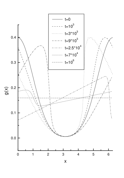
Figure 2: Seven snapshots of the generating function $g$ taken at different times. We have chosen as initial state a Gaussian distribution. Notice the appearance of the shock wave.

It is well-known that in general (91), (92) and (93) do not have continuous solutions for all time because shock waves appear after finite time and tend to dominate the solution as $t\to\infty$. The quantities $\int_{-\pi}^{\pi}g^{k}dx$ are preserved in time until a shock is formed. After a shock wave appears, only the mass $\int_{-\pi}^{\pi}g\;dx$ is conserved along the time evolution. Figure 2 is an illustration of the phenomenon. E. Hopf in [45] discussed the asymptotic behaviour for large time of solutions of (91)-(92). Later, P. D. Lax [46] and T. P. Liu and M. Pierre [47] completed and generalized this study for an arbitrary conservation law. A first result in this direction is given by the following inequality

$$|g^{H}(x,t)-M(x,t)|\ \leq\ c{2\pi\over t},$$ (94)

where $M(x,t)$ is the mean function

$$M(x,t)\ =\ {1\over 2\pi}\int_{-\pi}^{\pi}g^{H}(x,t)\ dx.$$

If $g_{0}$ is in $L^{\infty}_{2\pi}$, then the mean function is time independent and (94) holds.

Let us assume that initially $g_{0}(x)$ has a single maximum and a single minimum at each period. Then $g^{H}$ evolves towards a precise asymptotic shape so that its profile for large time looks like a 2$\pi$-periodic sawtooth profile with a single shock per period. Between shocks $g^{H}$ decreases linearly. The asymptotic behaviour profile result in the case of a Cauchy problem was specified by T. P. Liu and M. Pierre in [47]. By adapting the arguments in [47], we can prove for our periodic problem

$$\lim_{t\to\infty}t^{1\over 2p^{\prime}}\|g^{H}(\cdot,t)-\omega(\cdot,t)\|_{L^{p}_{2\pi}}\ =\ 0,$$

for an initial data $g_{0}\in L^{1}_{2\pi}$ and $1\leq p<\infty$. Here

$$\omega\left(x,t\right)\,=\,{1\over 2\pi}\,-\,{x\over 2K_{0}t}\,=\,-{1\over 2K_{0}t}\left(x-{K_{0}\over\pi}t\right)\qquad-\pi<x<\pi$$ (95)

which is a sawtooth profile moving towards the right at speed $K_{0}/\pi$. The strength of the shock $\mbox{max}(g)-\mbox{min}(g)=\pi/(K_{0}t)$ converges to zero as the time goes to infinity. Thus the shock weakens, it vanishes and we are left with the incoherent solution $(2\pi)^{-1}$. In summary, incoherence is the globally asymptotically stable solution for the periodic Burgers equation at any temperature, including zero. In the last case, interesting transient patterns including shock profiles are possible before every memory of the initial conditions is washed out.

7 The extended Burgers model

Instead of working with the nonlocal model given by Equations (54) and (60) for $g(x,t)$ we can try to find local equations for $v(x,t)$ and $g(x,t)$. Let us define

$$\rho(x,t)=2K_{0}\,[g(x,t)-g(x+\pi,t)],$$

$$\sigma(x,t)=2K_{0}\,[g(x,t)+g(x+\pi,t)].$$ (96)

These functions obey the equations (60) and

$$\frac{\partial\rho}{\partial t}=-\frac{\partial(\sigma v)}{\partial x}+T\frac{\partial^{2}\rho}{\partial x^{2}}\,,$$ (97)

$$\frac{\partial\sigma}{\partial t}=\frac{\partial}{\partial x}\Bigl{(}v\frac{\partial v}{\partial x}\Bigr{)}+T\frac{\partial^{2}\sigma}{\partial x^{2}}\,.$$ (98)

Now we can obtain an equation for $v(x,t)$ by inserting (61), i.e. $\partial v/\partial x=-\rho$ in (97), and integrating the result with respect to $x$:

$$\frac{\partial v}{\partial t}-\sigma v-T\frac{\partial^{2}v}{\partial x^{2}}=J(t)\,.$$ (99)

Equations (60) and (96) together with the periodicity of $g(x,t)$ imply that

$$\sigma(x+\pi,t)=\sigma(x,t),\quad v(x+\pi,t)=-v(x,t),$$ (100)

i.e. the $2\pi$-periodic functions $\sigma(\cdot,t)$ and $v(\cdot,t)$ are periodic and antiperiodic in the $x$ variable, respectively. Moreover the normalization condition for $g$ and the $\pi$-periodicity of $\sigma$ imply

$$\int_{0}^{\pi}\sigma(x,t)\ dx=2K_{0}.$$ (101)

The conditions (100) may be used to show that $J(t)\equiv 0$ in (99), so that $v$ obeys

$$\frac{\partial v}{\partial t}-\sigma v-T\frac{\partial^{2}v}{\partial x^{2}}=0\,.$$ (102)

To see this, substitute $x+\pi$ as the argument of $v$ and $\sigma$ in (99), and use (100) to obtain $J=-J$. Once $\sigma$ and $v$ are found, we obtain the generating function from the equation

$$g(x,t)={1\over 4K_{0}}\left[\sigma(x,t)-{\partial v(x,t)\over\partial x}\right].$$ (103)

A similar development to the study of the existence properties of solutions given for the Porous Medium and Burgers models can be done for $v(x,t)$ in (102). In fact, we can write

$$v(x,t)=\int_{-\pi}^{\pi}\Theta(x-z,t)v_{0}(z)\ dz$$

$$+\int_{-\pi}^{\pi}\int_{0}^{t}\Theta(x-z,t-s)\left(\sigma\,v\right)(z,s)\ dz\ ds$$ (104)

coupling it with

$$\sigma(x,t)=\int_{-\pi}^{\pi}\Theta(x-z,t)\sigma_{0}(z)\ dz\quad\quad\quad\quad\quad\quad\quad\quad$$

$$+\int_{-\pi}^{\pi}\int_{0}^{t}{\partial\Theta(x-z,t-s)\over\partial z}\left(v{\partial v\over\partial z}\right)(z,s)\ dz\ ds.$$ (105)

The same type of estimates as in the previous sections together with an iterative method and a fix point theorem lead to a cubic equation, instead of a quadratic one as in (76). This allows to ensure the existence and bounds in $L^{p}$, at least for small initial data in $L^{1}$, of both $v(x,t)$ and $\sigma(x,t)$, for positive temperature $T$. However, the Theta function does not appear with a space derivative in (104) as in the Porous Medium and Burgers models which implies the non-convergence in time towards its respective mean values.

For this extended Burgers model the asymptotic in time behaviour is described by the Liapunov functional analyzed in Section 3. Let us now find the stationary solutions of these equations. From (98) and (102), we obtain

$$\sigma v+T\frac{d^{2}v}{dx^{2}}=0,$$ (106)

$$T\sigma+{v^{2}\over 2}=L+Mx.$$

$\sigma(x)$ and $v(x)$ are $2\pi$-periodic functions obeying (100) and $L$ and $M$ are constants. $2\pi$-periodicity of $\sigma$ and $v$ imply that $M=0$ in the second of these expressions. Thus

$$T\sigma+{v^{2}\over 2}=L.$$ (107)

Now we have $L>0$ because $\sigma>0$. Combining (101) and (107), we find the following equation for $L$:

$$2TK_{0}+\int_{0}^{\pi}{v^{2}\over 2}\,dx=\pi L.$$ (108)

Inserting (107) into (106) we obtain

$$T^{2}\,\frac{d^{2}v}{dx^{2}}+\left(L-{v^{2}\over 2}\right)\,v=0.$$ (109)

This may be integrated once yielding

$${1\over 2}\,\left(\frac{dv}{dx}\right)^{2}+{Lv^{2}\over 2T^{2}}-{v^{4}\over 8T^{2}}={E\over T^{2}}\,.$$ (110)

The energy $E$, $0\leq E<L^{2}/2$ is calculated so that the period of $v(x)$ be $2\pi$. It is convenient to rewrite the previous equation in terms of

$$w(\xi)={v(x)\over\sqrt{L}}\,,\quad x={T\xi\over\sqrt{L}}\,.$$ (111)

Then (110) becomes

$${1\over 2}\,\left(\frac{dw}{d\xi}\right)^{2}+{w^{2}\over 2}-{w^{4}\over 8}={E\over L^{2}}\equiv{\cal E}.$$ (112)

Suppose that we choose $w(0)=0$, $w^{\prime}(0)>0$ as initial conditions for a given trajectory. Then $w(\xi)$ is

$$\int_{0}^{w(\xi)}{dw\over\sqrt{2{\cal E}-w^{2}+{w^{4}\over 4}}}=\xi,$$ (113)

until $v$ reaches the turning point $w_{0}({\cal E})$, where

$$w_{0}({\cal E})=\sqrt{2}\,\sqrt{1-\sqrt{1-2{\cal E}}}\,,$$ (114)

at $\xi=P({\cal E})/4$. Notice that we will obtain a one-parameter family of stationary solutions because $w(\xi+c)$, with $w(\xi)$ as in (113) and $c\in\hbox{{\rm I}\kern-1.99997pt\hbox{\rm R}}_{+}$, is also an admissible stationary solution. Because of symmetry, an oscillation period is first completed at four times this value, i.e., when

$$P({\cal E})=4\int_{0}^{w_{0}({\cal E})}{dw\over\sqrt{2{\cal E}-w^{2}+{w^{4}\over 4}}}={4\sqrt{2}\,K(m)\over\sqrt{1+\sqrt{1-2{\cal E}}}}\,,$$ (115)

$$m={1-\sqrt{1-2{\cal E}}\over 1+\sqrt{1-2{\cal E}}}\,.$$ (116)

Here $K(m)$ is the complete elliptic integral of the first kind with parameter $m$ given by (116); see [29], page 590. $P(\cal{E})$ is an increasing function from $P(0)=2\pi$ to $P(1/2)=+\infty$. Branches of admissible stationary solutions satisfy (100), in particular they fulfil $v(x+\pi)=-v(x)$. Then their energies ${\cal E}\in(0,1/2)$ should be such that

$$n\,P({\cal E})={2\pi\sqrt{L}\over T}\,,$$ (117)

for positive odd integers $n=2p-1$, $p=1,2,\ldots$. Notice that even $n$’s would yield inadmissible solutions such that $v(x+\pi)=+v(x)$. By changing to the $w$ and $\xi$ variables, Eq. (108) for $L$ may be written as

$$n\,\int_{0}^{w_{0}({\cal E})}{w^{2}dw\over\sqrt{2{\cal E}-w^{2}+{w^{4}\over 4}}}={\pi\sqrt{L}\over T}-{2K_{0}\over\sqrt{L}}$$ (118)

($n$ odd) or, equivalently, as

$$n\sqrt{8}\sqrt{1+\sqrt{1-2{\cal E}}}\,[K(m)-E(m)]={\pi\sqrt{L}\over T}-{2K_{0}\over\sqrt{L}}.$$ (119)

Here $E(m)$ is the complete elliptic integral of the second kind with parameter $m$ given by (116).

Given $K_{0}>0$ fixed, Equations (115), (117) and (119) yield the values of ${\cal E}$ and $L$ corresponding to a branch of stationary solutions with a given odd value of $n$. A given stationary solution $(n,{\cal E},L)$ will have $n$ maxima and $n$ minima. We can find $L$ from (117) and eliminate it in (119) with the result

$${4n^{2}\,K(m)\over\pi}\,\left[E(m)-{\sqrt{1-2{\cal E}}\,K(m)\over 1+\sqrt{1-2{\cal E}}}\right]={K_{0}\over T}\,.$$ (120)

This latter equation relates the energy ${\cal E}$ to the coupling parameter $K_{0}$. As $K_{0}$ increases so does the number of possible stationary branches. Notice that the stationary branch with index $n$ exists for values of the coupling constant larger than $K_{0}=n^{2}\,T\pi/2$. At this value, ${\cal E}=0$ (therefore, $m=0$). Clearly the number of possible stationary branches is then half the integer part of $\sqrt{2K_{0}/(\pi T)}$ (only odd $n$ are admissible), which increases with $K_{0}$. For a given stationary solution $v(x)$, the stationary probability density may be reconstructed from (103) as

$$g(x)={1\over 4K_{0}}\,\left\{{L\over T}-{v^{2}\over 2T}-{dv\over dx}\right\}\,.$$ (121)

A stationary periodic moment-generating function is given by (110), (111), (113), (117), (118), (120) and (121). Their explicit form may be obtained by using the definitions of the Jacobi elliptic functions; see [29], pages 569 and ss. From (111), (113), (117), (120) and (9), we find

$$v(x)={4nT\sqrt{m}K(m)\over\pi}\,\mbox{sn}u\,,$$ (122)

$$H(x)=-{n^{-1}\,m^{{1\over 2}}\over E(m)-{\sqrt{1-2{\cal E}}\,K(m)\over 1+\sqrt{1-2{\cal E}}}}\,\mbox{sn}u\,,$$ (123)

$$u={2nK(m)x\over\pi}\,.$$ (124)

The probability density may be reconstructed from (117), (120) – (124):

$$g(x)={K(m)\over 2\pi}\,{{1\over 1+\sqrt{1-2{\cal E}}}-m\,\mbox{sn}^{2}u-\sqrt{m}\,\mbox{cn}u\,\mbox{dn}u\over E(m)-{\sqrt{1-2{\cal E}}\,K(m)\over 1+\sqrt{1-2{\cal E}}}}\,.$$ (125)

Notice that these synchronized solutions are defined up to a constant phase shift $x\to x+c$, as we said before. Such solutions exist for any positive temperature $T>0$ if $K_{0}\geq n^{2}T\pi/2$. Therefore, it is possible to find synchronized solutions of the extended Burgers model for any positive temperature. The stationary drift velocity (122) has $n=2p-1$ ($p=1,2,\ldots$) maxima and $n$ minima on the interval $-\pi<x<\pi$. Between successive extrema, $v(x)$ vanishes once. According to (121), the extrema of $g(x)$ on the interval $(-\pi,\pi]$ are reached at the zeros of $v(x)$. A little algebra shows that

$${dg\over dx}={L^{{3\over 2}}\over 4K_{0}T^{2}}\,w(\xi)\,\left[1-{w^{2}\over 2}-{dw\over d\xi}\right]\,,$$

and thus

$${d^{2}g\over dx^{2}}\Big{|}_{v=0}={L^{2}\over 4K_{0}T^{3}}\,\left[{dw\over d\xi}-\left({dw\over d\xi}\right)^{2}\right]\,.$$

Since $dw/d\xi=\pm\sqrt{2{\cal E}}$ wherever $w=0$, we have

$$\mbox{sign}\left({d^{2}g\over dx^{2}}\right)\Big{|}_{v=0}=\mbox{sign}\left({dw\over d\xi}\right)\,.$$

Therefore maxima of $g(x)$ are reached at points where $v=0$ and $v^{\prime}(x)<0$. These zeros are $u=2lK(m)$, where $l$ is an odd number running from $-n+2$ to $n$. The corresponding values of $x$ are $x_{l,n}=l\pi/n$. Thus an oscillator population described by (122) is split in $n$ subpopulations with angles close to $x=x_{l,n}$, $l=-n+2,\ldots,n$. The frequency density is found by means of (18). In dimensionless form, $p_{n}(\Omega)=\sqrt{L}\,P_{n}(\sqrt{L}\Omega)$, which yields

$$p_{n}(\Omega) = {nTK(m)w_{0}({\cal E})\over 2\pi K_{0}\sqrt{2{\cal E}}}\sum_{w(\xi)=\Omega}\left\{{1-{\Omega^{2}\over 2}\over|w^{\prime}(\xi)|}-\mbox{sign}(w^{\prime}(\xi))\right\}\,.$$ (126)

Here the sum is over all solutions $\xi\in(-\pi,\pi]$ of the equation $w(\xi)=\Omega$. The maxima of $p_{n}(\Omega)$ yield the likeliest frequencies of rotation for the oscillators. See [8, 9] for additional physical interpretation and numerical simulations.

Once a stationary solution (with index $n$), $g(x)$ [equivalently we may specify $\sigma(x)$ and $v(x)$], has been found, it is interesting to discuss its linear stability. Let $\sigma(x,t)=\sigma(x)+e^{\lambda t}\hat{\sigma}(x)$, $v(x,t)=v(x)+e^{\lambda t}\hat{v}(x)$. Then $\hat{\sigma}$ and $\hat{v}$ satisfy (100), $\int_{0}^{\pi}\hat{\sigma}dx=0$, and solve:

$$-T\frac{d^{2}\hat{v}}{dx^{2}}-[\sigma(x)\hat{v}+v(x)\hat{\sigma}]=-\lambda\hat{v}\,,$$ (127)

$$-T\frac{d^{2}\hat{\sigma}}{dx^{2}}-\frac{d^{2}[v(x)\hat{v}]}{dx^{2}}=-\lambda\hat{\sigma}\,.$$ (128)

Solving these equations in the general case seems difficult. These equations are easy to solve for the incoherent solution $v(x)=0$, $\sigma(x)=2K_{0}/\pi$. In this case (127) and (128) uncouple and we explicitly find the eigenvalues

$$\lambda={2K_{0}\over\pi}-(2p-1)^{2}T,$$ (129)

$$\lambda=-(2p)^{2}T,$$ (130)

(where $p=1,2,\ldots$) corresponding to (127) and (128), respectively. Eq. (129) shows that incoherence is linearly unstable for $K_{0}>T\pi/2$. At $K_{0}=(2p-1)^{2}T\pi/2$ the stationary solutions (125) (with $n=1,3,\ldots$) bifurcate from the incoherent solution. This can also be checked as follows: linearize (109) about $v=0$ and calculate the value of $K_{0}$ for which there is a $2\pi$-periodic solution of the resulting equation which satisfies (100). It is $K_{0}=T\pi/2$ corresponding to $E=0$, $n=1$. This solution is linearly stable (at least for values of $K_{0}$ in an appropriately small half-neighbourhood of $T\pi/2$) because of the principle of exchange of stabilities between bifurcation branches. In figure 3 we show the different bifurcation branches which occur at different integer values of $n=2p-1$.

Figure 3: Bifurcation diagram ${\cal E}$ versus $2K_{0}/(\pi T)$ for stationary synchronized solutions branching off from incoherence ${\cal E}=0$ at the square of the odd integer numbers.

An alternative calculation of the first branch (index $n=1$) of stationary solutions bifurcating from incoherence is using Monte Carlo methods. They are quite powerful since acceptance rate can be tuned at will in such a way that the approach to the stationary state may be faster. Furthermore, the intrinsic dynamics in Monte Carlo methods is discrete in time, unlike the continuous-time dynamics of the original problem. Thus the rounding errors due to time discretization are absent in Monte Carlo calculations of stationary solutions. We use the Monte Carlo method and the Glauber algorithm with a random sequential updating of the phases for the model Hamiltonian (62) of Section 4.(d). Local phases are randomly changed from $\phi_{i}$ to $\phi_{i}+\alpha\delta$, where $\alpha$ takes values with equal probability on the interval $[0,1]$ and $\delta$ is the typical size of the move. The proposed change is accepted with probability $[1+\exp(\beta\Delta{\cal H})]^{-1}$ where $\Delta{\cal H}$ is the change in the Hamiltonian. A convenient synchronization order parameter $r$ is defined through the global magnetization $M=re^{i\alpha}=(1/N)\sum_{j=1}^{N}e^{i\phi_{j}}$. The order parameter can be calculated from Monte Carlo simulations of the Hamiltonian (41) with $E(x)=|x|$ and $K_{0}=1$; see figure 4. Notice that the curves in this figure tend to a curve intersecting the horizontal axis at the bifurcation point $T=2/\pi$ as $N$ increases. This corresponds to the expected bifurcation result for the NLFPE (dot-dashed line in Figure 4 corresponding to $N=\infty$). Notice that finite-size corrections are of order $N^{-{1\over 2}}$ far from the bifurcation point and of order $N^{-{1\over 4}}$ near it [19].

The transition temperature corresponding to the first branch is easily obtained through standard finite-size scaling methods. Consider the kurtosis (or Binder parameter) for the synchronization parameter $r$, $B=\frac{1}{2}(3-\frac{<r^{4}>}{<r^{2}>^{2}})$, where $<\ldots>$ is the standard configurational average [weighted with the usual Boltzmann-Gibbs factor, $\exp(-\beta{\cal H})$, and ${\cal H}$ is given by (62)]. The curves for $B$ are shown in figure 5 for different sizes. Note that these curves (specially for $N=50,100,500$, data for $N=1000$ is more noisy) intersect at a common point characterizing the bifurcation temperature.

Figure 4: Synchronization parameter $r$ as a function of $T$ for different sizes $N=50,100,500,1000,\infty$.

Figure 5: Binder parameter $B$ as a function of $T$ for different sizes (in the low $T$ region, from bottom to top) $N=50,100,500,1000$. The curves become steeper for larger values of $N$. The theoretical value of the bifurcation temperature $T=2/\pi$ is marked in the figure.

It is interesting to compare the present results with those of Daido’s order function theory [9]. Except for a constant factor, $-K_{0}^{-1}$, Daido’s order function is just $v(x,t)$ in our notation. Notice that as $K_{0}/T\to\infty$, (123) and (125) corresponding to the linearly stable solution with index $n=1$ become $H(x)=-$ sign$(x)$ and $g(x)=\delta(x-\pi)$, respectively. This coincides exactly with Daido’s solution at $T=0$ [11, 9]. An interesting aspect of our exact construction of stationary solutions is that they can shed some light on scaling near bifurcation points as $T\to 0$ [11, 9]. In fact, (120) implies that stationary solution branches issue forth from incoherence at $K_{0}=\kappa_{n}\equiv n^{2}\pi T/2$ ($n$ odd). Furthermore (120) shows that the $n$th synchronized stationary solution branch satisfies ${\cal E}\propto(K_{0}/T-n^{2}\pi/2)$ for $K_{0}/T$ close to its bifurcation value $K_{0}=\kappa_{n}$. Then (122) - (125) show that $g(x)=O(|K_{0}-\kappa_{c}|^{1/2})$ if $T>0$ ($\kappa_{c}$ stands for the value of the bifurcation parameter $K_{0}/T$ at the bifurcation point $\kappa_{n}$). Clearly as $T\to 0+$, a quasicontinuum of $N=O(\sqrt{K_{0}/T})$ stationary branches has bifurcated from incoherence for a small fixed $K_{0}$. In these circumstances, the derivation of a one-mode amplitude equation as in Ref. [11] does not describe correctly the situation. See [48] for a derivation of an amplitude partial differential equation describing a quasicontinuum of Hopf bifurcations; similar techniques could be used in the present case.

The results at zero temperature may be obtained in another form. The model with Daido coupling is described by (98), (102) and (103). Setting $T=0$ in these equations, we obtain an integro-differential equation

$${\partial v(x,t)\over\partial t}=v(x,t)\left\{\sigma_{0}(x)\,+\,\int_{0}^{t}{\partial\over\partial x}\left(v(x,s){\partial v(x,s)\over\partial x}\right)\,ds\right\}$$

which can be consider as a modification of the Porous Medium equation with memory. This equation can be also written in a local form in the following way:

$$\sigma={1\over v}\,{\partial v\over\partial t}\,,\quad{\partial\sigma\over\partial t}={1\over 2}\,{\partial^{2}v^{2}\over\partial x^{2}}\,.$$

Then $v(x,t)$ obeys

$${\partial\over\partial t}\left({1\over v}{\partial v\over\partial t}\right)={1\over 2}\,{\partial^{2}v^{2}\over\partial x^{2}}\,,$$ (131)

$${\partial^{2}u\over\partial t^{2}}={1\over 2}\,{\partial^{2}e^{2u}\over\partial x^{2}}\,,$$ (132)

if $|v|=e^{u}$. This is an amplitude equation with infinitely many terms (e.g., expand the exponential in a Taylor series), and $g(x,t)=O(K_{0})$ in agreement with Daido’s results: the critical exponent is $\beta=1$ if $g=O(|K_{0}-K_{c}|^{\beta})$. Nevertheless, (131) or (132) are very different from Crawford’s amplitude equations [11].

Clearly the stationary solutions of (131) compatible with the symmetry requirement $v(x+\pi,t)=-v(x,t)$ are $v_{0}(x)=q$ sign$(x)$, where $q$ is a constant. In particular, incoherence corresponds to $q=0$. $\sigma_{0}(x)$ obeys $\sigma v=0$. Thus $\sigma_{0}$ is zero except at the points where $v=0$, namely $x=0,\pi$ (mod. $2\pi$). If (101) holds and $\sigma(x+\pi)=\sigma(x)$, we have

$$\sigma_{0}(x)=2K_{0}[\delta(x)+\delta(x-\pi)],$$ (133)

on the interval $x\in(-\pi,\pi]$. Inserting $\partial v_{0}/\partial x=-2q\,[\delta(x)-\delta(x-\pi)]$ and (133) in (103), we obtain

$$g_{0}(x)=\delta(x-\pi),$$ (134)

provided $q=K_{0}$. This density function is the same as that obtained above by taking the limit $K_{0}/T\to\infty$ of the stable stationary density with index $n=1$. Daido found the same results by using his order function theory [9]. Notice that the stationary solution (134) is a member of the one-parameter family of stationary solutions, $g_{0}(x+c)$, $c=$ constant.

Linearization of (98) and (102) (with $T=0$) about $v_{0}(x)=K_{0}$ sign$(x)$ and (133), $v(x,t)=v_{0}(x)+V(x,t)$, $\sigma(x,t)=\sigma_{0}(x)+\Sigma(x,t)$ ($V\ll v_{0}$, $\Sigma\ll\sigma_{0}$), yields

$${\partial V\over\partial t}=\sigma_{0}(x)\,V+v_{0}(x)\,\Sigma,$$ (135)

$${\partial\Sigma\over\partial t}={\partial v_{0}(x)V\over\partial x}\,,$$ (136)

which is equivalent to

$${\partial^{2}W\over\partial t^{2}}-\sigma_{0}(x)\,{\partial W\over\partial t}=K_{0}^{2}\,{\partial W\over\partial x}\,,$$ (137)

$$W(x,t)=v_{0}(x)\,V(x,t).$$ (138)

If we prove that $W(x,t)$ evolves towards zero as $e^{-Mt^{2}}$, $M>0$, then this implies that the density (134) is linearly stable. But analyzing Equation (137) as a Heat equation with respect to $t$, with boundary conditions $W\to 0$ as $|t|\to\infty$, we have the Green function of the linear part

$$\tilde{\Gamma}(x,t)\ =\ (4\pi K_{0}^{-2}|x|)^{-{1\over 2}}e^{-{K_{0}^{2}|t|^{2}\over 4|x|}},\ x>0.$$

Using the periodicity and symmetry properties of $v$ and $\sigma$, the solution can be written in convolution form with respect to $t$ with initial data $K_{0}V(0,t)$. This allows to assure that $W(x,t)$ evolves towards zero as $e^{-Mt^{2}}$, with $M=K_{0}^{2}/4\pi$.

8 Concluding remarks

In this paper, we have considered the Kuramoto model for synchronization of phase oscillators with global periodic coupling functions $f(x)$ and subject to external random forces. For general couplings and natural frequency distributions, we have derived the one-oscillator nonlinear Fokker-Planck equation and given an approximate formula for its solution in the limit of high natural frequencies. Provided the frequency distribution has $m$ peaks in the high-frequency limit, this formula indicates that the one-oscillator probability density splits into $m$ components. Each component corresponds to the solution of a NLFPE with zero natural frequency, on a frame rotating with fixed angular velocity. Which results do we know for such a reduced zero-frequency NLFPE?

In Section 3, we have shown that a Liapunov functional of the free energy type exists for a class of odd coupling functions (zero natural frequency). Then the probability density evolves towards a stable stationary function. Which stationary function this is, depends on $f(x)$. We have analyzed a family of singular coupling functions for which the NLFPE reduces to partial differential equations or systems thereof, such as the porous media equation, the Burgers equation or systems of Burgers equations. For these equations, we have examined the behavior of their solutions in the limit of large times for different temperatures; see Section 4 for details. The most interesting coupling function, $f(x)=$ sign $x$ (periodically extended outside $[-\pi,\pi]$), was already studied by Daido in the case of zero temperature, $T=0$ (see Section 2.2 for a rephrasing of his assumptions and results). This model is capable of synchronization at any temperature. We have found exact formulas for stationary synchronized probability densities which bifurcate supercritically from incoherence. Although we have not been able to determine their linear stability, we know that the first bifurcating branch of solutions is stable at least for coupling parameter near the bifurcation point. Let us assume that this bifurcating branch is always stable for coupling parameter above the bifurcation value. We can combine our results to obtain the stable probability density for a model with a multimodal natural frequency distribution in the high-frequency limit. We find that, except for a constant shift in $x$, the stable probability density is

$$\rho\sim\sum_{l=1}^{m}\rho^{(0)}_{l}(x-\Omega_{l}\omega_{0}t),$$ (139)

$$\rho^{(0)}_{l}(x)=\theta\left({\pi T\over 2}-K_{0}\alpha_{l}\right)\,{1\over 2\pi}+\theta\left(K_{0}\alpha_{l}-{\pi T\over 2}\right)\,g(x;K_{0}\alpha_{l}),$$ (140)

where $\theta(x)$ is the Heaviside unit step function. In these equations, $g(x;K_{0}\alpha_{l})$ is the solution (125) corresponding to setting $n=1$ and $K_{0}\alpha_{l}$ instead of $K_{0}$ in (120). The overall velocity function (proportional to Daido’s order function) is a superposition of rotating waves correponding to the contributions of the synchronized components

$$v(x,t) \sim \sum_{l=1}^{m}\alpha_{l}\,\theta\left(K_{0}\alpha_{l}-{\pi T\over 2}\right)\,{4T\sqrt{m_{l}}K(m_{l})\over\pi}\,$$ (141)

$$\times \mbox{sn}\left({2K(m_{l})\,(x-\Omega_{l}\omega_{0}t)\over\pi}\right)\,.$$

Here $m_{l}$ is the value of $m$ obtained by substituting $n=1$ and $K_{0}\alpha_{l}$ instead of $K_{0}$ in (120).

Appendix A A convolution identity for the velocity

To obtain the convolution identity (8), we can write the velocity $v(x,t)$ as follows

$$v(x,t) = -K_{0}\sum_{n=-\infty}^{\infty}a_{n}H_{-n}^{0}e^{inx}$$

$$= -K_{0}\sum_{n=-\infty}^{\infty}\left({1\over 2\pi}\int_{-\pi}^{\pi}e^{-inx^{\prime}}f(x^{\prime})dx^{\prime}\right)H_{-n}^{0}e^{inx}$$

$$= -K_{0}{1\over 2\pi}\int_{-\pi}^{\pi}f(x^{\prime})\sum_{n=-\infty}^{\infty}e^{in(x-x^{\prime})}H_{-n}^{0}\ dx^{\prime}$$

which, using the expression for $g(x,t)$

$$g(x,t)={1\over 2\pi}\,\sum_{n=-\infty}^{\infty}H_{n}^{0}e^{-inx}={1\over 2\pi}\,\sum_{n=-\infty}^{\infty}H_{-n}^{0}e^{inx},$$

gives the announced relationship (8).

Appendix B Order function and oscillator drift velocity

In our notation, Daido’s order function is defined as [39]

$$H(x,t)=-\sum_{k=-\infty}^{\infty}h_{k}Z_{k}e^{-ikx}\,,$$

where Daido’s coupling function is related to ours by $h(x)=-f(-x)$ ($h_{k}=-a_{-k}$), and

$$Z_{k}(t)={1\over N}\,\sum_{j=1}^{N}e^{ik[\phi_{j}(t)-\Omega_{e}t]}=\int_{-\pi}^{\pi}e^{ikx}\left({1\over N}\,\sum_{j=1}^{N}\delta(\phi_{j}(t)-\Omega_{e}t-x)\right)\,dx$$

$$=\int_{-\pi}^{\pi}e^{ikx}g(x+\Omega_{e}t,0,t)dx.$$

Here we have used that $N^{-1}\sum_{j=1}^{N}\delta(\phi_{j}(t)-x)$ tends to $g(x,0,t)$ in the limit of infinitely many oscillators. Thus $Z_{k}(t)$ is $2\pi$ times the Fourier coefficient of $g(x+\Omega_{e}t,0,t)$ with index $-k$. Inserting this in $H(x,t)$ above, we find

$$H(x,t)=-\int_{-\pi}^{\pi}g(x^{\prime}+\Omega_{e}t,0,t)\left(\sum_{k=-\infty}^{\infty}h_{k}\,e^{ik(x^{\prime}-x)}\right)dx^{\prime}$$

$$=-\int_{-\pi}^{\pi}g(x^{\prime}+\Omega_{e}t,0,t)\,h(x^{\prime}-x)\,dx^{\prime}=\int_{-\pi}^{\pi}g(x^{\prime}+\Omega_{e}t,0,t)\,f(x-x^{\prime})\,dx^{\prime}$$

$$=\int_{-\pi}^{\pi}g(x+\Omega_{e}t-x^{\prime},0,t)\,f(x^{\prime})\,dx^{\prime},$$

which, together with (8), implies

$$H(x,t)=-{1\over K_{0}}\,v(x+\Omega_{e}t,t).$$

Then (9) follows, as said in the Introduction.

Acknowledgments The authors want to express their gratitude to Rafael Ortega and Juan L. Vázquez for useful discussions and for pointing them some references. We acknowledge partial support by the DGES (Spain) Projects PB98-0142-C04-01 (LLB) and PB98-1281 (JS), FOM (The Netherlands) contract FOM-67596 and DGES (Spain) contract PB97-0971 (FR) and TMR (European Union) contract ERB FMBX-CT97-0157 (LLB & JS).

References

References

- [1] A.T. Winfree, Geometry of Biological Time, Springer-Verlag, New York (1990).
- [2] Y. Kuramoto, Self-entrainment of a population of coupled nonlinear oscillators, in International Symposium of Mathematical Problems in Theoretical Physics, H. Araki ed., Lecture Notes in Physics, Vol.39 (Springer, New York), (1975) 420-422.
- [3] S. Shinomoto and Y. Kuramoto, Phase transitions in active rotator systems, Prog. Theor. Phys. 75, (1986) 1105-1110.
- [4] Y. Kuramoto and I. Nishikawa, Statistical macrodynamics of large dynamical systems. Case of a phase transition in oscillator communities, J. Stat. Phys. 49, (1987) 569-605.
- [5] Y. Kuramoto, Chemical Oscillations, Waves and Turbulence, Springer, Berlin (1984).
- [6] S. H. Strogatz, Norbert Wiener’s brain waves, in Lect. N. Biomath. 100, edited by S. Levin, Springer, N. Y. 1994.
- [7] K. Wiesenfeld, P. Colet, and S.H. Strogatz, Synchronization transitions in a disordered Josephson series array, Phys. Rev. Lett. 76, (1996) 404-407.
- [8] H. Daido, Order function and macroscopic mutual entrainment in uniformly coupled limit-cycle oscillators, Prog. Theor. Phys. 88 (1992), 1213-1218.
- [9] H. Daido, A solvable model of coupled limit-cycle oscillators exhibiting partial perfect synchrony and novel frequency spectra, Physica D 69 (1993), 394-403.
- [10] H. Daido, Onset of cooperative entrainment in limit-cycle oscillators with uniform all-to-all interactions: bifurcation of the order function, Physica D 91 (1996), 24-66.
- [11] J. D. Crawford, Scaling and singularities in the entrainment of globally coupled oscillators, Phys. Rev. Lett. 74 (1995), 4341-4344. See also J. D. Crawford and K.T.R. Davies, Synchronization of globally-coupled phase oscillators: singularities and scaling for general couplings. Physica D 125 (1999), 1-46.
- [12] L. L. Bonilla, C. Pérez-Vicente, F. Ritort and J. Soler, Exactly solvable phase oscillator models with synchronization dynamics, Phys. Rev. Lett. 81 (1998), 3643-3646.
- [13] C. J. Pérez-Vicente and F. Ritort, A moment-based approach to the dynamical solution of the Kuramoto model, J. Phys. A (Math. Gen.) 30 (1997), 8095-8103.
- [14] F. Ritort, Solvable dynamics in a system of interacting random tops, Phys. Rev. Lett. 80 (1998), 6-9.
- [15] J. D. Crawford, Amplitude expansions for instabilities in populations of globally-coupled oscillators, J. Stat. Phys. 74 (1994), 1047-1084.
- [16] L. L. Bonilla, C. Pérez-Vicente and R. Spigler, Time-periodic phases in populations of nonlinearly coupled oscillators with bimodal frequency distributions, Physica D 113 (1998), 79-97.
- [17] J. A. Acebrón and L. L. Bonilla, Asymptotic description of transients and synchronized states of globally coupled oscillators, Physica D 114 (1998), 296-314.
- [18] L. L. Bonilla, Stable Probability Densities and Phase Transitions for Mean-Field Models in the Thermodynamic Limit, J. Stat. Phys. 46, (1987) 659-678.
- [19] D. A. Dawson, Critical dynamics and fluctuations for a mean-field model of cooperative behavior, J. Stat. Phys. 31 (1983), 29-85.
- [20] P. Dai Prá and F. den Hollander, McKean-Vlasov limit for interacting random processes in random media, J. Statist. Phys. 84 (1996), 735-772.
- [21] L. L. Bonilla, J. C. Neu and R. Spigler, Nonlinear stability of incoherence and collective synchronization in a population of coupled oscillators, J. Stat. Phys. 67 (1992), 313-330.
- [22] L. L. Bonilla, C. J. Pérez Vicente and R. Spigler, Time-periodic phases in populations of nonlinearly coupled oscillators with bimodal frequency distributions, Physica D 113 (1998), 79-97.
- [23] L. L. Bonilla, J. A. Carrillo and J. Soler, H-theorem for electrostatic or self-gravitating Vlasov-Poisson-Fokker-Planck systems, Phys. Lett. A 212 (1996), 55-59.
- [24] L. L. Bonilla, J. A. Carrillo and J. Soler, Asymptotic behavior of an initial-boundary value problem for the Vlasov-Poisson-Fokker-Planck system, SIAM J. Appl. Math. 57 (1997), 1343-1372.
- [25] J. M. Kim and J. M. Kosterlitz, Growth in a restricted solid-on-solid model, Phys. Rev. Lett. 62 (1989), 2289-2292.
- [26] O. A. Ladyženskaja, V. A. Solonnikov, N. N. Ural’ceva, Linear and quasilinear equations of parabolic type, Translations of Mathematical Monographs 23, AMS, Providence, 1968.
- [27] S. N. Kruzhkov, Periodic solutions to non-linear equations, Differential’-nye Uravnenija, 6 (1970), 731-740.
- [28] G. B. Folland, Introduction to PDEs. Princeton U. P., Princeton, 1976.
- [29] M. Abramowitz and I.A. Stegun, Handbook of Mathematical Functions. Dover, N. Y., 1965.
- [30] D. V. Widder, “The Heat Equation”, Academic Press, New York-San Francisco-London, 1975.
- [31] O. Vejvoda, “Partial differential equations: time periodic solutions”, Martinus Nijhoff Publishers, The Hague-Boston-London, 1982.
- [32] G. H. Cottet and J. Soler, Three-dimensional Navier-Stokes equations for singular filament data, J. Diff. Equations 74 (1988), 234-253.
- [33] Ya. Zel’dovich, A. S. Kompaneets, Theory of heat transfer with temperature dependent thermal conductivity, in Collection in honour of the 70th birthday of academician A. F. Ioffe, Izdvo. Akad. Nauk SSSR, Moscow (1950), 61-71.
- [34] G. I. Barenblatt, On some unsteady motions of a liquid gas in a porous medium, Prikl. Mat. Mekh. 16 (1952) 67-78.
- [35] O. Oleǐnik, S.A. Kalashnikov, Y. L. Czhou, The Cauchy problem and boundary-value problems for equations of the type of unsteady filtration, Izv. Akad. Nauk SSSR, Ser. Mat. 22 (1958), 667-704.
- [36] A. S. Kalashnikov, Some problems of the qualitative theory of non-linear degenerate second-order parabolic equations, Russian Math. Surveys 42 (1987), 169-222.
- [37] J. L. Vázquez, An introduction to the mathematical theory of the porous medium equation, in “Shape Optimization and Free Boundaries”, M. C. Delfour ed., Math. and Phys. Sciences, Series C, vol. 380, Kluver Acad. Publ., Dordrecht-Boston-Leiden (1992), 347-389.
- [38] L. A. Peletier, The Porous Medium Equation, in “Applications of Nonlinear Analysis in the Physical Sciences”, H. Amann et al. eds., Pitman, London (1981), 229-241.
- [39] C. M. Dafermos, Asymptotic behavior of solutions of evolution equations, (M. G. Crandall, Ed.) Academic Press, New York, 1978.
- [40] N. D. Alikakos and R. Rostamian, Large Time Behavior of Solutions of Neumann Boundary Value Problem for the Porous Medium Equation, Indiana U. Math, J. 30 (1981), 749-785.
- [41] E. Godlewski, P. A. Raviart, Hyperbolic systems of conservation laws, SMAI 3/4, Paris, 1991.
- [42] A. Parker, On periodic solution of the Burgers equation: a unified approach, Proc. R. Soc. Lond. A 438 (1992), 113-132.
- [43] K. L. OuYoung, Periodic Solutions of Conservation Laws, J. Math. Anal. Appl. 75 (1980), 180-202.
- [44] S. N. Kruzhkov, First order quasilinear equations in several independent variables, Math. USSR-Sb. 10 (1970), 217-243.
- [45] E. Hopf, The partial differential equation , Comm. Pure Appl. Math. 3 (1950), 201-230.
- [46] P. D. Lax, Hyperbolic systems of conservation laws II, Comm. Pure Appl. Math. 10 (1957), 537-566.
- [47] T. P. Liu and M. Pierre, Source-Solutions and Asymptotic Behavior in Conservation Laws, J. Diff. Equations 51 (1984), 419-441.
- [48] L. L. Bonilla and F. J. Higuera, The Onset and End of the Gunn Effect in Extrinsic Semiconductors, SIAM J. Appl. Math. 55 (1995), 1625-1649.