A quasi-diagonal approach to the estimation of Lyapunov spectra
for spatio-temporal systems from multivariate time series

Abstract

We describe methods of estimating the entire Lyapunov spectrum of a spatially extended system from multivariate time-series observations. Provided that the coupling in the system is short range, the Jacobian has a banded structure and can be estimated using spatially localised reconstructions in low embedding dimensions. This circumvents the “curse of dimensionality” that prevents the accurate reconstruction of high-dimensional dynamics from observed time series. The technique is illustrated using coupled map lattices as prototype models for spatio-temporal chaos and is found to work even when the coupling is not strictly local but only exponentially decaying.

]

Contents

toc

I Introduction

One of the most important tools for investigating chaotic dynamical systems is the spectrum of Lyapunov exponents. These exponents measure the asymptotic exponential divergence or convergence of two infinitesimally close orbits. In this paper we are interested in estimating all of the Lyapunov exponents of a spatio-temporal system from an observed multivariate time-series without prior knowledge of the dynamics governing the system. Hitherto, most efforts in this area have concentrated on only estimating the largest (or few largest) exponent(s). However, at least some of the negative exponents are needed if we wish to estimate the dimension of the attractor via the Kaplan-Yorke conjecture. Estimating all of the Lyapunov exponents from a time series for spatially extended systems is a daunting task. The fundamental problem is the high dimensionality of the system which prevents an accurate reconstruction of the dynamics from observed data. In particular, whatever method of function approximation we use to reconstruct the dynamics, we need to have a reasonable spread of data in the region of interest. Thus, for instance, a local linear or quadratic approach estimates the value of a function at a point $y\in{{R}}^{d}$ by performing a linear least squares regression in a neighbourhood of $y$. Such a neighbourhood must contain a sufficient number of data points to yield a meaningful estimate and yet not be so large that the function is no longer linear (or quadratic respectively). As $d$ grows, more and more data is necessary to ensure that sufficient numbers of neighbours can be found and for $d$ much larger than 6 or so the amount of data required becomes completely impracticable. This problem is often informally referred to as the “curse of dimensionality”.

It is therefore perhaps surprising that, at least in some cases, the whole Lyapunov spectrum can be estimated successfully from observed data, see Ref. [3] and [4]. Both of these papers focus on a lattice of locally coupled fully chaotic logistic maps, though Ref. [4] (here referred as ORS99) also considers the effects of skewing the map (as we also do below in VI), and of replacing it by a much more non-linear function. The results for the latter two cases are substantially less satisfactory than for the standard logistic map. It turns out that the key property that makes it possible to obtain reasonable estimates of the spectrum for the logistic map lattice using the methods in ORS99 is that the dynamics at one spatial location is easily approximated within the space of functions used to fit the dynamics. Hence what at first sight appears to be a local quadratic fit is in fact a global fit. This allows the “curse of dimensionality” to be circumvented, and good estimates of the dynamics to be obtained even in high dimensions. As the local dynamics moves away from the space of functions used to fit the dynamics the estimates of the Lyapunov spectrum rapidly deteriorate. One approach to overcoming this might be to attempt to estimate the local dynamics and then use a suitable basis to fit the dynamics[5].

The alternative, which is the method used in Ref. [3] (here referred as BH99) and which we pursue here, is based on the observation that as long as the spatial coupling in the system is reasonably short range, optimal predictions are often obtained in very low embedding dimensions[6], even when the dimensionality of the attractor is high. This somewhat counter-intuitive result may be explained by the rapid spatial decay of the dependence of the dynamics at one site on its neighbours[7]. This suggests that it ought to be possible to obtain reasonable estimates of the Jacobian by performing appropriate fits in low embedding dimensions, hence avoiding the “curse of dimensionality”.

The aim of this manuscript is to describe a method based on this intuitive idea and evaluate its performance in various circumstances. The method is based on only reconstructing the non-zero entries of the Jacobian in a row-by-row fashion. More precisely if the coupling in a spatio-temporal system is reasonably local then the only non-zero entries in the Jacobian are near the diagonal. Rather than estimating the whole Jacobian, one should only estimate the non-zero entries (which can be done in a low embedding dimension) and set the remaining entries to 0. We call such an approach a quasi-diagonal one. Essentially the same technique is used by Bünner and Hegger in BH99 who successfully apply it to the logistic coupled map lattice, using local linear fits. However, as ORS99 shows, the standard logistic lattice is a relatively easy system for which to estimate the spectrum, even using local linear fits (rather than quadratic ones, as in ORS99 and here). It is thus impossible to judge from BH99 how well a quasi-diagonal approach works when the local dynamics presents a bigger challenge, or indeed when the coupling is anything but nearest neighbour. Finally, ORS99 demonstrates that dramatically improved estimates of the spectrum can be obtained by truncating the outer layer(s) of the estimated Jacobian, thereby eliminating boundary effects. Such truncation is not considered in BH99.

The present work combines the best features of BH99 and ORS99 together with additional generalisations and extensive supporting numerical evidence. In particular, we evaluate the quasi-diagonal approach when applied to a more difficult local map, using a more flexible (quadratic) fitting basis. We investigate the effect of truncating the outer layers of the estimated Jacobian and assess the effectiveness of our approach when the coupling is exponentially decaying, rather than just nearest neighbour. The encouraging numerical results we obtain motivate us to present a possible extension of the quasi-diagonal approach to continuous space-time extended dynamical systems (i.e. partial differential equations).

For the convenience of the reader, we present our approach in a largely self-contained manner, leading in a natural progression from a scalar method, which gives very poor results, to a successful quasi-diagonal estimation of the Jacobian from multivariate time series. In the process we highlight the relationship between the “globality” of the fitting basis and the “curse of dimensionality”. We also emphasise the importance of properly addressing the effects of the boundaries of the subsystem where we collect the multivariate time series.

The paper is organised as follows. The next section gives a general introduction to spatio-temporal systems and describes the prototype model (a coupled map lattice) that is used in our numerical investigations. In section III we provide a short overview of Lyapunov spectra for extended dynamical systems and their relationship to fractal dimensions and the Kolmogorov-Sinai entropy. We give some examples and explain how to estimate the Lyapunov spectrum from subsystem information using a suitable rescaling. In the following section (IV) we attempt to estimate the Lyapunov spectrum using a scalar time series. We find that the lack of spatial information hinders any attempt to obtain a meaningful reconstruction of the dynamics, and hence to estimate the spectrum. In section V we present a systematic numerical study of estimates of the Lyapunov spectrum using different spatio-temporal reconstructions. We discover the importance of including spatial information in order to obtain reasonable reconstructions of the dynamics. We also point out that boundary effects on the measured subsystem have to be properly addressed by truncating the outer layer(s) of the estimated Jacobian. In section VI we turn our attention to the effect of passing from a local fit to a global fit when increasing the embedding dimension of the spatio-temporal reconstruction. We conclude that the “curse of dimensionality” precludes any hope of a usable reconstruction when our fitting basis does not give a good global approximation to the dynamics. We then go on in section VII to exploit the sparse structure of the Jacobian when the coupling is short range to develop a quasi-diagonal estimation technique for the Jacobian. Additionally, we use the spatial homogeneity of the system to dramatically increase the amount of effective data points available when performing a local fit. This circumvents both the “curse of dimensionality” and the error induced by not using an appropriate global basis. Section VIII is devoted to the generalisation of our approach to systems that have non-local, but exponentially decaying coupling. Finally, in the last section, we propose a natural extension of our method to the estimation of the Lyapunov spectra of partial differential equations.

II Spatially extended systems

The occurrence of chaos in spatio-temporal systems has recently attracted the attention of a large part of the dynamical systems community. There exists nowadays a broad understanding of low-dimensional chaotic systems. However, the same cannot be said of high-dimensional systems and in particular of spatially extended systems. The addition of a spatial extent to the dynamics produces a complex interplay between the local dynamics (the original dynamics before including spatial interactions) and the spatial interactions. Sometimes, this interplay triggers the so called phenomenon of spatio-temporal chaos. Loosely speaking, this refers to systems that combine a familiar temporal chaotic evolution with an additional decay of spatial correlations. In a spatio-temporal chaotic regime both space translations and time evolutions exhibit instabilities and it is even possible to define spatial and temporal Lyapunov exponents[8]. One possible simple mechanism for obtaining spatio-temporal chaotic motion is to spatially couple low-dimensional chaotic units; although one has to be careful because the coupling sometimes tends to reduce the spatio-temporal instabilities[9]. However, it is also possible to produce spatio-temporal chaos through the spatial interaction of well-behaved (non-chaotic) units. This is the case for some metapopulation dynamics models[10].

In contrast with non-spatially distributed systems, spatio-temporal systems possess a spatial extent. This may be discrete, giving a lattice with a local dynamical unit at each site, or continuous. The typical model in the latter case (if time is also continuous) is a partial differential equation (PDE). By discretising space we obtain a lattice of ordinary differential equations (commonly referred to as a lattice differential equation). In the discrete space case, the system can be viewed as a collection of low dimensional dynamical systems coupled together via some spatial rule (for a review of current research see Ref. [11]). Examples of this kind of model are widespread in the literature, particularly in the field of solid state physics where they are used to study the dynamics of interacting atoms arranged in a lattice (see Ref. [12] and references therein).

In this paper we focus our attention on a third category of extended dynamical systems where not only space but also time is discrete. In such a case the model consists of low-dimensional dynamical units with discrete time (i.e. maps) arranged in some discrete lattice configuration in one or more spatial dimensions. Such models are usually called coupled map lattices (CMLs). They were first introduced in 1984 as simple models for spatio-temporal complexity[13, 14, 15]. Despite their computational simplicity, CMLs are able to reproduce a wide variety of spatio-temporal behaviour, such as intermittency[16], turbulence[17, 18] and pattern formation[19], to name just a few.

In this paper we shall focus on a one-dimensional array of sites. The length of this array could be infinite but here we restrict ourselves to an array of length $N$ with periodic boundary conditions. At the $i$-th site we introduce a discrete time local dynamical system whose state at time $n$ we denote by $x_{i}^{n}$. We suppose that the same local map $f$ acts at every spatial location (so that the local dynamics is homogeneous). In the simplest case, the local variable $x_{i}^{n}$ is taken to be one-dimensional. The dynamics of the CML is then a combination of the local dynamics and the coupling, which consists of a weighted sum over some spatial neighbourhood. The time evolution of the $i$-th variable is thus given by

$$x^{n+1}_{i}=\sum_{k}\varepsilon_{k}f(x^{n}_{i+k}),$$ (1)

where the range of summation defines the neighbourhood. The coupling parameters $\varepsilon_{k}$ are site-independent, and satisfy $\sum\varepsilon_{k}=1$. The commonest choice for the coupling scheme is

$$x^{n+1}_{i}=(1-\varepsilon)f(x^{n}_{i})\displaystyle+{\varepsilon\over 2}\left(f(x^{n}_{i-1})+f(x^{n}_{i+1})\right),$$ (2)

which is sometimes called a diffusive CML. This is a discrete analogue of a reaction-diffusion equation. There is now a single coupling parameter $\varepsilon$ which is constrained by the inequality $0\leq\varepsilon\leq 1$, to ensure that the signs of the coupling coefficients in (2) (i.e. $\varepsilon/2$ and $1-\varepsilon$) remain positive.

III Lyapunov spectra for extended dynamical systems

Let us now give an overview on the extraction and application of Lyapunov spectra for spatio-temporal systems. For a $N$-dimensional dynamical system there exist $N$ Lyapunov exponents which in principle can be obtained from the eigenvalues of the matrix

$$\Gamma=\lim_{n\rightarrow\infty}{\left[P(n)^{\rm tr}\cdot P(n)\right]^{1/2n}},$$ (3)

where $P(n)$ corresponds to the product of the first $n$ Jacobians along the orbit and $(\,\cdot\,)^{\rm tr}$ denotes matrix transpose. It is well known that given an invariant measure (which is usually assumed to be the natural measure for the dynamics) the Multiplicative Ergodic Theorem (e.g. Ref. [20]) ensures that the limit exists for almost all initial conditions $x^{0}$, and if the measure is ergodic then its eigenvalues are independent of $x^{0}$. The Lyapunov exponents are then defined as the logarithms of these eigenvalues (which are obviously non-negative). Although computing the exponents using equation (3) appears straightforward, in practice multiplying the Jacobians is an ill-conditioned procedure since the most expanding direction swamps all the other expansion/contraction rates. Therefore one has to resort to algorithms that regularly reorthogonalise the product of the Jacobians. Such algorithms perform a QR decomposition every few iterates and are closely related to standard methods of computing eigenvalues[21]. The QR decomposition can be carried out using Gram-Schmidt, Householder or Givens based techniques. In this paper we use an efficient Householder method where only the terms required for the computation of the Lyapunov exponents are actually calculated[22].

We define the Lyapunov spectrum (LS) as the set of Lyapunov exponents $\{\lambda_{i}\}_{i=1}^{N}$ arranged in decreasing order. The LS not only gives the expansion/contraction rates of infinitesimal perturbations, but can also provide estimates of fractal dimensions and entropies. Thus, for instance, the dimension of the chaotic attractor (i.e. informally the effective number of degrees of freedom) is given by the Kaplan-Yorke conjecture[23] through the Lyapunov dimension

$$D_{L}=j+{1\over|\lambda_{j+1}|}\sum_{i=1}^{j}\lambda_{i},$$ (4)

where $j$ is the largest integer for which $\sum_{i=1}^{j}\lambda_{i}>0$. It is also possible to extract an upper bound for the Kolmogorov-Sinai (KS) entropy $h$ from the LS by the following approximation[20]

$$h=\sum\lambda_{i}^{+},$$ (5)

where the summation is over the positive Lyapunov exponents $\lambda_{i}^{+}$. The KS entropy quantifies the mean rate of information production in a system, or alternatively the mean rate of growth of uncertainty due to infinitesimal perturbations.

As an example, figure 1.a shows the LS for a coupled logistic lattice of size $N=20$ with periodic boundary conditions obtained using the known dynamics (2). In figure 1.b we plot the sum of the Lyapunov exponents $\sum_{k=1}^{i}\lambda_{k}$ from where the KS entropy can be estimated (maximum of the curve) and the Lyapunov dimension can be extracted (intersection with the horizontal axis). Notice that the Lyapunov dimension $D_{L}\simeq 15.4$ is comparable to the total size of the lattice $N=20$. Also observe that $D_{L}\simeq 15.4$ implies the presence of a high dimensional attractor. This point will be addressed in more detail in the following sections.

The computation of the whole LS for spatio-temporal systems is a cumbersome task, particularly as the size of the system increases. Even the most efficient methods involve ${\mathcal{O}}(N^{3})$ arithmetic operations per time step[21] for a lattice of size $N$. Even for moderate lattice sizes ($N\sim 50$) the number of operations required is already considerable. Moreover, taking into account that sometimes the (time) convergence of the Lyapunov exponents is extremely slow, the time necessary to compute the whole LS for spatio-temporal systems quickly becomes prohibitive. Furthermore, one is often interested in the behaviour of the system in the thermodynamic limit where the number of lattice sites $N$ goes to infinity. In such a case it quickly becomes impossible to compute the whole LS and one has to resort to subsystem rescaling techniques that we shall now briefly describe.

FIG. 1.: a) Lyapunov spectrum for a CML of $N=20$ fully chaotic logistic maps $f(x)=4x(1-x)$ with coupling strength $\varepsilon=0.4$. b) The Lyapunov dimension $D_{L}$ and the KS entropy $h$ may be estimated from the sum of the Lyapunov exponents. In this case the largest Lyapunov exponent is $\lambda_{1}\simeq 0.36$, $D_{L}\simeq 15.4$ and $h\simeq 1.8$.

Consider a one-dimensional lattice of coupled one-dimensional dynamical units. High dimensional cases may be treated in a similar way. Assume the array is large ($N\gg 1$) and suppose initially that it is made up of smaller independent (uncoupled) subsystems of size $N_{s}$. For simplicity take $N$ to be a multiple of $N_{s}$. The LS of the whole lattice then consists of $N/N_{s}$ exact copies (assuming spatial homogeneity) of the subsystem LS of $N_{s}$ Lyapunov exponents. Thus, the LS for the whole lattice consists of $N_{s}$ Lyapunov exponents, each with multiplicity $N/N_{s}$. As we relax the assumption that the subsystems are uncoupled we hope that the LS does not change significantly[24, 25]. If this is the case, the whole LS of the original lattice may be approximated by a rescaled version of its subsystem LS.

An obvious choice for such a rescaling is to multiply the index $i$ of the $N_{s}$-subsystem Lyapunov exponents $\lambda_{i}(N_{s})$ by $r^{\prime}=N/N_{s}$. However, careful analysis of the LS of a homogeneous state suggests that a better rescaling for one-dimensional lattices is given by[26]

$$r={N+1\over N_{s}+1}.$$ (6)

The rescaling of the whole LS from subsystem information leads us naturally to define intensive quantities from extensive quantities. As a direct consequence of this rescaling, using the same argument as in the previous paragraph, it is straightforward to see that the Lyapunov dimension and the KS entropy are extensive quantities (i.e. $D_{L}$ and $h$ increase linearly with $N$). Moreover, it is useful to introduce their respective densities by simply dividing them by the system volume (lattice size)[27]. This even allows such quantities to be defined in the thermodynamic limit, although care has to be taken in doing this for systems such as PDEs where space is continuous[28].

By using subsystem rescaling one can considerably reduce the computing resources required to estimate the whole LS of a large spatio-temporal system. Furthermore, by restricting oneself to observing data from a subsystem, one reduces the dimensionality of the resulting time series and increases the likelihood of success in applying reconstruction techniques.

IV Lyapunov spectra from univariate time series

In the previous section we assumed that the dynamics of the system whose LS we wished to compute was known. This is not the case for many complex physical systems. We therefore now turn to the task of estimating the LS when the only information available about the system is a time series of observed data. Let us start by applying standard delay reconstruction techniques for a single observable time-series. Thus suppose that the univariate time series $\{\varphi^{n}\}$ has been measured from a $k$ dimensional system. We can create a high dimensional reconstructed state space by constructing the delay vectors

$$y^{n}=(\varphi^{n},\varphi^{n-1},\dots,\varphi^{n-(d-1)}),$$ (7)

where $d$ is the so-called embedding dimension. Takens’ Theorem[29] says that for $d\geq 2k+1$, the dynamics induced on such delay vectors is generically smoothly conjugate to the original dynamics. This apparently arbitrary condition is a simple geometrical disentangling in order to avoid self intersections on the reconstructed manifold[30]. The smooth conjugacy between induced and original dynamics asserts that the time series contains all the coordinate-free properties of a dynamical system. Specifically, since the LS is invariant under smooth conjugacy (i.e. smooth coordinate changes) the LS computed from the dynamics of the delay vectors will be the same as that of the original system. Note that the time series need not to be the time history of one of the system’s state variables but can be any generic function of the state of the system. In particular, in principle it is possible to reconstruct all the Lyapunov exponents from a univariate time series. To anyone familiar with the proof of Takens’ Theorem is it obvious that it generalises straightforwardly to multi-variate time series, though as far as we are aware, a proof has never appeared in the literature.

Unfortunately, Takens’ Theorem does not actually apply to the CMLs considered here[6]. Firstly, the maps that we use as local dynamics are not invertible, and the proof of Takens’ Theorem depends fundamentally on such invertibility. Secondly, we assume translation invariance of the CML (i.e. the dynamics and coupling are spatially homogeneous) and such symmetry renders our systems far from generic. Finally, in a similar fashion, measurement functions depending on only a single site (or group of sites) are not generic in the space of all observables, indeed a generic function will depend on all $N$ sites. On the other hand our results, and in particular the comparison with the LS computed in the previous section assuming full knowledge of the actual dynamics, suggest that we are able to estimate the real LS from observed time series. We shall therefore use delay reconstruction techniques throughout this paper without worrying about this failure of Takens’ Theorem (and in any case the theorem only draws conclusions for generic dynamics and measurement functions, and so cannot guarantee reconstruction for any particular time series).

For the extended dynamical systems we are considering, the dimension $k$ is the size of the lattice $N$ times the dimension of the local dynamics. Hence for the logistic coupled map lattice in figure 1 we get $k=N$. Even for quite moderate $N$ an embedding dimension of $2N+1$ is clearly quite impractical. Of course, the condition $d\geq 2k+1$ is only a sufficient one, and it is well known that some systems (e.g. the Lorenz equations) can be reconstructed for smaller values of $d$. Furthermore, Sauer and Yorke[31] have a sharper estimate for $d$ that is still sufficient to preserve the box-counting dimension and the Lyapunov exponents

$$d>D_{B}+D_{T},$$ (8)

where $D_{B}$ is the box-counting dimension of the attractor and $D_{T}$ is a “tangent dimension” which is informally the maximum (over all points) dimension of the tangent space of the underlying dynamics. However even this is still very prohibitive. For example, for the system in figure 1) the Lyapunov dimension for even quite a small lattice of $N=20$ coupled logistic maps we have $D_{L}\sim 15.4$. Then assuming $D_{B}=D_{L}$ (i.e. essentially the original Kaplan-Yorke conjecture), the bound (8) gives $d>15.4+D_{T}$, and one would typically expect $D_{T}$ to lie between $D_{B}$ and $N$, giving a value of $d$ from 30 upwards. Of course the Sauer-Yorke inequality is also just a sufficient condition, but if one is to preserve all $N$ exponents, it seems that an absolute minimum of $d\geq N$ will be necessary, and even this is too large to be generally practicable.

FIG. 2.: Estimates of the LS for a logistic coupled map lattice of size $N=20$ and coupling $\varepsilon=0.4$ computed using a time delay reconstruction (with $d\in[32,42]$) from a univariate time series (thin lines). A second order local fit from a sample of $10^{4}$ points was used and the number of neighbours was set to the number of parameters in the fitting process plus 20. For comparison the spectrum computed from the original dynamics is depicted with a thick line. An orbit length of $10^{4}$ iterations was used in both cases and the computed LS was rescaled using (6).

Indeed, as indicated in the introduction, an embedding dimension much larger than $d\sim 6$ will lead to the so-called “curse of dimensionality”. Thus in order to estimate the LS from the time series we need to approximate the map that governs the dynamics of the delay vectors, that is the map $F$ such that $F(y^{n})=y^{n+1}$. There exist several methods for doing this, of which the best for the purpose at hand are all based on local approximations. These can be constructed by scanning the time series to find a set of past close encounters (corresponding to neighbours in the reconstructed state space) of the current reconstructed state $y^{n}$. Once these neighbours have been found, an approximation $\hat{F}$ to $F$ at $y^{n}$ can be computed using, for example, a least squares fit within an appropriate space of functions (e.g. linear or quadratic). For a comprehensive review see the recent book by Kantz and Schreiber[32]. For large embedding dimensions ($d\sim 6$) it becomes extremely difficult to find close neighbours and hence, due to data limitations, the approximation to $F$ ceases to be local. This in turn can lead to large errors in the determination of the Lyapunov exponents.

It is clear then that function approximation techniques are bound to fail when reconstructing spatio-temporal systems where the dynamics is typically high dimensional. As an example figure 2 shows the results of an attempt to estimate the whole LS from a univariate time series obtained from a single site of a couple logistic lattice. The measurement function in this case is the projection onto a single site, so that $\varphi^{n}=x_{j}^{n}$ for a fixed $j$. An embedding dimension in the range $32\leq d\leq 42$ was used. It is obvious from the figure that this temporal delay reconstruction of the LS (overlapping thin lines) completely fails to reproduce the LS of the original system (thick line). Other values of the reconstruction parameters than the ones given in the figure caption were also tried yielding the same qualitative results.

V Lyapunov spectra from spatio-temporal data

Since the direct application of univariate (temporal) delay reconstructions clearly fails for spatio-temporal systems, let us now try to exploit the spatial extent of the system and use a spatio-temporal delay reconstruction. The framework for this is presented in[6]. Here, we shall show the benefits of including spatial information in estimating the LS. We shall also investigate the advantages of truncating the outer layer of a reconstructed Jacobian in order to avoid boundary effects. We have already addressed these issues in a previous paper[4], however we repeat some of the analysis here for completeness.

A spatio-temporal reconstruction is obtained by replacing the delay vectors (7) of the previous section by the spatio-temporal delay vectors

$$y^{n}_{i}=(\phi^{n}_{i},\phi^{n}_{i-1},\dots,\phi^{n}_{i-(d_{s}-1)}),$$ (9)

whose entries $\phi^{n}_{i}=(x_{i}^{n},x_{i}^{n-1},\dots,x_{i}^{n-(d_{t}-1)})$ are time-delay vectors and the spatial index $i$ is fixed. The overall embedding dimension for such a spatio-temporal reconstruction is $d=d_{s}d_{t}$, where $d_{s}$ and $d_{t}$ denote the spatial and temporal embedding dimensions respectively. The standard temporal delay reconstruction (7) is recovered by setting $d_{s}=1$. Spatio-temporal reconstructions have proved useful in various contexts[33, 34, 35]. By adding the extra spatial delay in the time series one is including important information that is otherwise very difficult to obtain. In fact, it is extremely difficult to extract information about neighbouring dynamics just by doing spatially localised measurements. This is because of the rapid decay of spatial correlations in locally coupled extended dynamical systems. In a previous paper[7] we showed how this extremely rapid decay in correlations allows a quite small truncated lattice with random inputs at the boundaries to reproduce the local dynamics of a large, potentially infinite, lattice. This tends to suggest that a univariate time series cannot in practice reconstruct the dynamics of a whole spatio-temporal system.

FIG. 3.: LS estimated from spatio-temporal delay reconstructions for a logistic coupled map lattice. The LS computed from the original dynamics is depicted with a thick line while the different spatio-temporal delay reconstructions are depicted with dashed lines. All the fitting parameters are the same as in figure 2 (second order fitting, $10^{4}$ points, $10^{4}$ iterates).

In figure 3 we present several estimates of the LS of the coupled logistic lattice (as in figure 2) for different spatio-temporal embedding dimensions $d$. The different reconstructions correspond to a broad sample of choices of $d_{s}$ and $d_{t}$. Note that simply increasing $d=d_{s}d_{t}$ does not improve the estimates. In fact, in order to get a good estimate of the LS, it seems preferable to take $d_{t}=1$ and $d_{s}$ as large as possible. This is indicated by the empty and filled circles corresponding to $d_{t}=1$ and $d_{s}=10$ and $d_{s}=20$ respectively. In the figure we show only a few combinations of $(d_{s},d_{t})$. However, we originally considered a much broader choice without finding any qualitative differences. We therefore conclude that a spatio-temporal reconstruction with $d_{t}=1$ (that is a pure spatial delay reconstruction) gives the best results. This is easy to explain since we are using the actual dynamical variables of the system ($\varphi_{i}^{n}=x_{i}^{n}$) as observables and are measuring them in a complete window. Thus, we do not need to increase the embedding dimension to avoid self intersection in the reconstructed space since we are already in a natural space for the system.

FIG. 4.: LS estimated from pure spatial delay reconstructions for a logistic coupled map lattice. All the fitting parameters are the same as in figure 2 (second order fitting, $10^{4}$ points, $10^{4}$ iterates).

In figure 4 we show the reconstruction of the LS using a pure spatial reconstruction with increasing $d_{s}$. These estimates are much more promising than before. Note that since our original system is of size $N=20$ it is not possible to choose $d_{s}>20$. Indeed, we have to be careful, since taking $d_{t}=1$ and $d_{s}=N=20$ corresponds to measuring the whole state space and is therefore not a genuine delay reconstruction. This explains why the reconstructed LS for $d_{t}=1$ and $d_{s}=N=20$ agrees so well with the direct computations (triangles in figure 4) though note that in figure 1 we know the Jacobian of the dynamics exactly, whilst here we still have to do some function fitting.

From figure 4 we see that as $d_{s}$ is increased a better estimate of the LS is obtained. One may think that this is simply the effect of getting a higher embedding dimension. However, the reason for the apparent convergence of the reconstructed LS towards the exact LS as $d_{s}\rightarrow N$ is simply due to a reduction of the noise from boundary effects. Consider the sites at the boundary of our spatial window in which we measure the multivariate time series. The dynamics of these sites depends on sites whose evolution is not explicitly contained in the measurement window. As a consequence, the estimates of the Jacobian for these sites contain spurious terms and are subject to error. For instance, the fitting procedure for the first row tries to compensate for the lack of information from the left neighbouring site that is outside of the measurement window by including an artificial dependence on all sites inside the window. This will yield erroneous non-zero terms off the tri-diagonal.

FIG. 5.: LS estimated from pure spatial delay reconstructions for a logistic coupled map lattice using truncation of the outer layer of the Jacobian. All the fitting parameters are the same as in figure 2 (second order fitting, $10^{4}$ points, $10^{4}$ iterates).

We can avoid these effects by observing that the boundary sites contribute towards the Jacobian at its outer rows and columns. We can therefore remove such boundary effects by simply truncating the outer rows and columns of the reconstructed Jacobian to yield a $(d_{s}-2)\times(d_{s}-2)$ matrix[4]. Note that one must first fit the $d_{s}\times d_{s}$ Jacobian and only then truncate its outer rows and columns. Also observe that for a spatial delay embedding dimension $d_{s}$ we obtain $d_{s}-2$ Lyapunov exponents. The results of applying this technique are shown in figure 5. Comparing this to figure 4 where the outer layer of the Jacobian was not truncated we see a dramatic improvement, and in particular can obtain good estimates even for quite small $d_{s}$ (see also Ref. [4]). It is obvious that the truncation of the outer layer of the Jacobian has to coincide with the range of the coupling: the larger the coupling range the more outer rows and columns must be truncated. This is considered further below in section VIII.

VI Local versus global fitting: a matter of dimensionality

It is somewhat surprising that the estimated LS in figure 5 are in such good agreement with the actual LS despite the fact that the embedding dimensions are a) too small to disentangle the state space and b) too large to avoid the “curse of dimensionality”. The explanation for this apparent contradiction is that the measurement functions are the actual variables of the system and the form of the dynamical equations is actually contained in the space spanned by the basis functions used to approximate them. In particular, the dynamics of our CML is quadratic in nature (c.f. equation (2) with logistic local maps) and we are using a quadratic fit. Thus, a local fit is in fact also a global one and the problem of not finding enough neighbours in high-dimensions is avoided. It thus turns out to be possible to obtain very good estimates of the dynamics with even moderate amounts of data.

FIG. 6.: Skewed logistic map (thick line) for for $b=0.2$ obtained by applying (10) to the fully chaotic logistic map (dashed line).

This situation is however unlikely to arise in most real applications, and typically we expect that the (delay reconstructed) dynamics will not lie in the space spanned by the basis functions. To investigate the effects of this we now turn our attention to a skewed logistic local map which yields a CML whose dynamics is not contained in the space of quadratic polynomial functions that we use for fitting. This map is obtained from the standard logistic map $f(x)=ax(1-x)$ by applying the following skew transformation of the unit square

$$K(x,y)=(x+by,y),$$ (10)

where $b$ is a parameter determining the degree of skew. In this way we obtain the map (figure 6)

$$g_{b}(x)={-1+ab(2x-1)+\sqrt{(1+ab)^{2}-4abx}\over 2ab^{2}},$$ (11)

where $b$ must satisfy $-1/a<b<1/a$ so that the derivatives of $g_{b}$ at 0 and 1 remain bounded.

FIG. 7.: Estimation of the LS for a coupled map lattice of skewed logistic maps. The size of the lattice is $N=20$, the coupling parameter is $\varepsilon=0.4$ and the skew parameter is $b=0.2$. The original LS is indicated by the solid line and the estimates using a range of spatial embedding dimensions $d_{s}$ are depicted by various symbols. For large $d_{s}$ the estimates deteriorate because of the “curse of dimensionality”. All the fitting parameters are the same as in figure 2 (second order fitting, $10^{4}$ points, $10^{4}$ iterates).

We now repeat the estimation of the LS for this skewed map. Figure 7 shows the effects of increasing the spatial embedding dimension $d_{s}$ in the case of large skew $b=0.2$. Observe that for small $d_{s}$ ($\leq 6$) the approximation of the LS is quite good (see square points in figure). However, as $d_{s}$ increases, the estimate deteriorates. This reflects the fact that as the embedding dimension grows the fitting algorithm has more and more difficulty finding close neighbours. Since the skewed logistic map cannot be well approximated globally by a quadratic function the LS estimate deteriorates. Note however that even though an accurate estimate of the LS is not possible in this case, the estimated LS does have the right qualitative features. This is due to the fact that the skewed logistic map still resembles a quadratic function to some extent and thus a global fit is still reasonable. This is illustrated in figure 8 where we present the effect of varying the degree of skew $b$, and hence the degree of departure from the space of quadratic functions. We see that as the skew is increased, the error between the actual and the estimated LS rapidly increases. Using a local map which is even further from the space of quadratic ones leads to yet greater discrepancies[4].

Finally recall also that the number of Lyapunov exponents obtained for a given $d_{s}$ is $d_{s}-2$ due to the truncation of the outer layers of the Jacobian. Therefore if we try an avoid the “curse of dimensionality” by working in low embedding dimensions with $d_{s}\leq 6$ we obtain only 4 points or less on the LS density curve. Even if these are accurate, we cannot in general expect to extrapolate the whole spectrum from just these 4 points. Hence estimates of Lyapunov dimension and KS entropy are likely to be quite poor[4].

FIG. 8.: Effect of the skew of the local map when estimating the LS. Curves correspond to the LS computed with the known dynamics and the symbols depict various pure spatial delay reconstructions. All the fitting parameters are the same as in figure 2 (second order fitting, $10^{4}$ points, $10^{4}$ iterates).

The results presented in this section suggest that as soon as the dynamics cannot be globally approximated by the space spanned by the basis functions used in the fit, and as soon as more than a handful of Lyapunov exponents is required, standard spatio-temporal embedding techniques cannot reliably estimate the LS. In the next section we shall show how this difficulty can be overcome by focusing on the estimation of only the nontrivial entries in the Jacobian. An alternative approach is to try and find an adapted fitting basis that will allow us to fit the dynamics globally. This can be done by first extracting an estimate of the local dynamics from the time series and then using this to construct an appropriate set of basis functions. One possible way of estimating the local dynamics is to use time-delay plots[4]. An even more promising technique is to consider quasi-homogeneous states in a small window and their time evolution[5].

VII Quasi-diagonal reconstruction of the Jacobian

In this section we improve the method presented above by making use of the local nature of the coupling in our CML, which results in the Jacobian exhibiting a banded-diagonal structure. It is thus natural to only attempt to estimate the non-zero entries in this Jacobian. We call this a quasi-diagonal reconstruction. This allows us to carry out the local fit in a low dimensional space, and avoids the difficulties described above. A similar idea was employed by Bünner and Hegger[3]. However, they only applied it to a standard logistic CML, which as we have seen above is a relatively easy system for which to estimate the spectrum using conventional means. It is thus impossible to judge from their work how much of a benefit the quasi-diagonal approach actually brings. Additionally, here we combine this technique with a truncation of the outer layers of the Jacobian, which, as we have seen above, brings substantial benefits, but was not considered in[3].

The idea behind a quasi-diagonal reconstruction of the Jacobian is quite simple. The entries of the Jacobian $J(n)$ at time $n$ are given by

$$J_{kl}(n)={\partial x^{n+1}_{k}\over\partial x^{n}_{l}}.$$ (12)

Due to our assumption of localised coupling most of these terms are identically zero. The only non-zero terms lie within a distance of the diagonal given by the distance over which the coupling acts. In the particular case of a nearest neighbour CML (2), the Jacobian is tri-diagonal, and has only three non-zero elements in each row:

$$J(n)=\pmatrix{\partial^{1}_{1}&\partial^{1}_{2}&0&&\phantom{\ddots}&0\cr\partial^{2}_{1}&\partial^{2}_{2}&\partial^{2}_{3}&0&&\phantom{\ddots}\cr 0&\ddots&\ddots&\ddots&0&\cr&0&\ddots&\ddots&\ddots&0\cr&&0&\ddots&\ddots&\partial^{d_{s}-1}_{d_{s}}\cr 0&\phantom{\ddots}&&0&\partial^{d_{s}}_{d_{s}-1}&\partial^{d_{s}}_{d_{s}}~{}~{}~{}\cr},$$ (13)

where, for simplicity, we use the notation:

$$\partial^{u}_{v}={{\partial x^{n+1}_{i_{0}+u-1}}\over{\partial x^{n}_{i_{0}+v-1}}}$$

Note that the Jacobian (13) is extracted from sites $i_{0}$ to $i_{0}+d_{s}-1$ and so is of size $d_{s}\times d_{s}$. The starting index $i_{0}$ is arbitrary since we are assuming spatial homogeneity.

We estimate this Jacobian in a row by row fashion by fitting local dynamics of the form

$$x_{r}^{n+1}=F_{r}(x_{r-1}^{n},x_{r}^{n},x_{r+1}^{n}).$$ (14)

for $(1<r<d_{s})$. This fit is carried out in just a three dimensional space, as opposed to a $d_{s}$ dimensional as before, and close neighbours are defined by their distance from $(x_{r-1}^{n},x_{r}^{n},x_{r+1}^{n})$. This thus avoids any problems with high-dimensionality. Furthermore, if the dynamics is translation invariant (i.e. spatially homogeneous), we can use any triple of the form $(x_{j-1}^{n},x_{j}^{n},x_{j+1}^{n})$, regardless of position. This dramatically increases the effective amount of data available to us for performing the fit. Additionally, if the dynamics is also isotropic, i.e. invariant under the symmetry that exchanges $x_{j}^{n}$ with $x_{N-j}^{n}$, we can use all triples in reverse order $(x_{j+1}^{n},x_{j}^{n},x_{j-1}^{n})$. Of course, if the coupling acts over a longer range then the map $F_{r}$ will depend on more variables, but as long as the coupling remains reasonably local this approach will still bring advantages (we investigate this further in the next section).

FIG. 9.: Effect of truncating the outer row of the Jacobian for a tri-diagonal estimate of the LS for a lattice of coupled skewed logistic maps as in figures 7 and 8. The skew is $b=0.2$ and the width of the window used to extract the multivariate time series is $d_{s}$ sites. The open symbols correspond to using the whole fitted Jacobian while the solid symbols correspond to truncating the outer layer of the Jacobian. All the fitting parameters are the same as in figure 2 (second order fitting, $10^{4}$ points, $10^{4}$ iterates).

The first and last rows of $J(n)$ contain only two non-zero entries due to the lack of information from outside the observation window. As before, the entries will be estimated incorrectly since the fitting algorithm will try and compensate for the lack of the missing entry by erroneously adjusting the remaining two. We therefore truncate the outer layers of the Jacobian as in the previous section and compute only $d_{s}-2$ Lyapunov exponents from a window of size $d_{s}$. The improvements due to such truncation are shown in figure 9. Note that these become less apparent as the width $d_{s}$ of the observation window increases. This is consistent with the fact that the boundary effects become less significant as the size of the subsystem grows[7]. Nevertheless, given that it always leads to better estimates, we shall continue to employ such truncation throughout the remainder of the paper.

FIG. 10.: Tri-diagonal estimate of the LS for a lattice of coupled skewed logistic maps as in figures 7 and 8. The skew is $b=0.2$ and the width of the window used to extract the multivariate time series is 20 sites. All the fitting parameters are the same as in figure 2 (second order fitting, $10^{4}$ points).

Figure 10 shows an example of the estimation of the LS using a quasi-diagonal reconstruction with a large window $d_{s}=20$. Compared to figures 7 and 8 we see that this approach can give an excellent estimate, even though the local map cannot be well approximated by a quadratic fit. Similar results where obtained for different maps and coupling strengths.

VIII Estimating the Lyapunov spectrum for exponentially decaying coupling

The CML used to illustrate our method in the previous sections only allowed interactions between nearest neighbours. There are however many other systems of interest where the coupling acts over greater distances. In this section we investigate the performance of our approach in such cases. Typically, it is assumed that the coupling decreases in strength with distance, giving a band-diagonal Jacobian with sub-diagonals whose entries decay as we move away from the diagonal. A suitable paradigm model to represent this is a CML where the coupling range is in fact infinite but whose coupling coefficients decay exponentially with distance:

$$x^{n+1}_{i}={1-\beta\over 1+\beta}\sum_{k=-\infty}^{\infty}{\beta^{|i-k|}f(x^{n}_{i-k})},$$ (15)

where the coupling parameter $\beta\in(0,1)$. The limit $\beta\rightarrow 0$ corresponds to the uncoupled case, i.e. $x^{n+1}_{i}$ depends only on $x^{n}_{i-k}$. The limit $\beta\rightarrow 1$ corresponds to global coupling of all the sites with the same coefficient. Thus increasing $\beta$ effectively increases the range of the coupling and results in more and more sub-diagonals of the Jacobian becoming significant. Whilst for $\beta$ close to 0, it is reasonable to expect that a tri-diagonal reconstruction will still suffice, it is clear that as $\beta$ increases, more sub-diagonals will need to be taken into account.

We thus investigated the effects of using a higher-diagonal reconstruction for data from a lattice with a relatively large $\beta$ (0.35). If we fix the size $q$ of the admissible interaction range we need to estimate a map depending on $2q+1$ variables:

$$F_{r}^{(q)}(x_{r-q}^{n}\dots,x_{r-1}^{n},x_{r}^{n},x_{r+1}^{n},\dots,x_{r+q}^{n})=x_{r}^{n+1},$$ (16)

FIG. 11.: Estimation of the LS using a $(2q+1)$-diagonal reconstruction of the Jacobian for a lattice of coupled skewed logistic maps with decaying exponential coupling (15). The skew is $b=0.2$ and the decay rate is $\beta=0.35$. The coupling parameters for $\beta=0.35$ correspond to $\varepsilon_{0}\simeq 0.481$, $\varepsilon_{\pm 1}\simeq 0.168$, $\varepsilon_{\pm 2}\simeq 0.059$, $\varepsilon_{\pm 3}\simeq 0.021$, $\varepsilon_{\pm 4}\simeq 0.007$, …, in the general CML formulation (1). All the fitting parameters are the same as in figure 2 (second order fitting, $10^{4}$ points, $10^{4}$ points).

We now need to discard $q$ outer layers of the estimated Jacobian to remove boundary effects, and hence if our observation window is of size $d_{s}$, we can estimate $d_{s}-2q$ Lyapunov exponents.

Figure 11 shows the results of this approach applied to the CML coupling scheme (15) for different values of $q$ (still with a skewed logistic map for local dynamics). We see that the tri-diagonal ($q=1$) reconstruction completely fails to approximate the LS. However, as $q$ increases the reconstruction rapidly improves. For $q=2$ the largest Lyapunov exponents are captured accurately and the estimate of the remainder of the spectrum is still quite poor. This improves significantly for $q=3$ and $q=4$ where the approximation is rather good, particularly given that the coupling is not genuinely over a finite range. Increasing $q$ further led to a deterioration of the estimates of the LS. This is due to the reappearance of the “curse of dimensionality”: for $q\geq 5$ we have to find neighbours in dimension $d=2q+1\geq 11$. We repeated these experiments for other values of $\beta$ and other local maps, obtaining similar qualitative results.

IX Discussion and generalisations

We have shown that by using a quasi-diagonal reconstruction of the Jacobian we are able to estimate the LS of a variety of CML’s using only time series data with a reasonable degree of accuracy. The most difficult test was where the local dynamics was given by a skewed logistic map and the coupling was exponentially decaying. In that case, we had to take a 9-diagonal reconstruction of the Jacobian (i.e. $q=4$). Increasing $q$ beyond this leads to increasing errors, due to the increase in the dimensionality of the reconstruction space that we use. We therefore have a dichotomy when trying to estimate LS for systems with extended interactions: on the one hand we would like to include as many sub-diagonals as possible (i.e. $q$ as large as possible), however, on the other hand, $q$ cannot be chosen too large ($q\leq 5$) otherwise we again encounter the “curse of dimensionality”.

Of course, in practice if we do not know the dynamics of a system, we are unlikely to know a priori the range of the coupling. However, this is something that can be estimated from a multivariate time series, using for example some kind of cross correlation. This in turn will allow us to estimate the width of the band of the Jacobian that is most appropriate to capture the essence of these interactions.

A related problem arises when trying to reconstruct LS from multivariate time series produced by systems with a continuous space variable, or when probing real life extended dynamical systems. Consider for example a one-dimensional PDE and assume that we are free to choose the sampling intervals in both time and space at which data is observed. The Jacobian will contain a different number of significant sub-diagonals depending on the choice of these intervals. This is illustrated in figure 12 where we show the so called cone-horizon for the evolution of a perturbation in space-time. The cone-horizon corresponds to the region of space-time where a perturbation, applied at the summit of the cone, can influence downstream positions. Any point outside the cone-horizon cannot “feel” the presence of the disturbance. Such cone-horizons always exist for extended dynamical systems where the interactions have finite range, i.e. where information propagation has finite speed. Now suppose that we observe the system at regular intervals in space and time. This corresponds to the the intersections of the grid shown in the figure. Let us denote by $\tau$ the temporal sampling; for simplicity we assume the spatial sampling interval is fixed, since varying $\tau$ is sufficient to demonstrate our point. For the example depicted in the figure a sampling interval of $\tau$ yields a tri-diagonal Jacobian. This is because there are only three sites in the cone-horizon after a time $\tau$. Thus, for this choice of space-time discretisation it should be sufficient to use a tri-diagonal reconstruction of the Jacobian, i.e. with $q=1$. However, if we double the sampling interval to $2\tau$ we shall need to use a 5-diagonal reconstruction in order to include the 5 sites in the cone-horizon after a time $2\tau$.

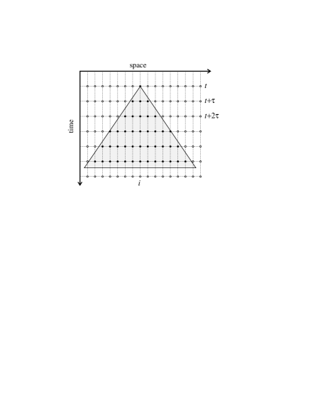
FIG. 12.: Cone-horizon for a disturbance in a one-dimensional, space-time continuous, extended dynamical system. A disturbance applied at the summit of the cone may alter the downstream dynamics inside the cone-horizon (shaded area). Applying a given space-time discretisation (dashed mesh) induces a particular neighbourhood structure: a node at time $t+\tau$ depends on a fixed number of nodes at time $t$ (3 in this case). The slope of the cone-horizon fixes the number of sub-diagonals required in the quasi-diagonal estimation of the Jacobians.

We intend to investigate the application of the quasi-diagonal method to the estimation of a LS from a time series generated by a PDE in a future paper. Additionally, we have hitherto assumed that the observable is the actual state variable at a site. This is unlikely to be the case in many practical applications. In such a case, we expect that the best approach would be a combination of the quasi-diagonal reconstruction method presented here with a local spatio-temporal reconstruction of the dynamics.

We would like to thank D.S. Broomhead, J. Huke and T. Schreiber for useful discussions. This work was carried out under a UK Engineering and Physical Sciences Research Council grant (GR/L42513). JS would also like to thank the Royal Society, the Leverhume Trust and the Royal Commission for the Exhibition of 1851 for financial support.

REFERENCES

- [1] Present address: Department of Mathematics and Statistics, Simon Fraser University, BC, Canada V5A 1S6. E-mail: ricardo_carretero@sfu.ca, URL: http://www.math.sfu.ca/rcarrete/ric.html
- [2] URL: http://www.ucl.ac.uk/CNDA
- [3] M.J. Bünner and R. Hegger. Estimation of Lyapunov spectra from space-time data. Phys. Lett. A, 258, 1 (1999) 25-30.
- [4] S. Ørstavik, R. Carretero-González and J. Stark. Estimation of intensive measures in spatio-temporal systems from time-series Submitted to Physica D, 1999.
- [5] R. Carretero-González. Extracting local dynamics from extended dynamical systems: a times-series reconstruction perspective. In preparation, 2000. Preprint version:http://www.ucl.ac.uk/ucesrca/abstracts.html.
- [6] S. Ørstavik and J. Stark. Reconstruction and cross-prediction in coupled map lattices using spatio-temporal embedding techniques. Phys. Lett. A, 247 (1998) 146–160.
- [7] R. Carretero-González, S. Ørstavik, J. Huke, D.S. Broomhead and J. Stark. Thermodynamic limit from small lattices of coupled maps. Phys. Rev. Lett., 83 (1999) 3633–3636.
- [8] S. Lepri, A. Politi and A. Torcini. Chronotopic Lyapunov Analysis. J. Stat. Phys., 82, 5/6 (1996) 1429–1452.
- [9] Y. Braiman, J.F. Lindner, W.L. Ditto. Taming spatiotemporal chaos with disorder. Nature, 378, 6556 (1995) 465–467.
- [10] P. Rohani and O. Miramontes. Host-parasitoid metapopulations: the consequences of parasitoid aggregation on spatial dynamics and searching efficiency. Proc. R. Soc. Lond. B., 260 (1995) 335–342.
- [11] Lattice Dynamics. In Proceedings of the Workshop on Lattice Dynamics, Paris, 21–23 June 1995. Physica D, 103, 1997.
- [12] P. Poggi and S. Ruffo. Exact solutions in the FPU oscillator chain. Physica D, 103 (1997) 251–272.
- [13] K. Kaneko. Period-doubling of kink-antikink patterns, quasiperiodicity in anti-ferro-like structures and spatial intermittency in coupled logistic lattice. Prog. Theor. Phys., 72, 3 (1984) 480–486.
- [14] I. Waller and R. Kapral. Spatial and temporal structure in systems of coupled nonlinear oscillators. Phys. Rev. A, 30, 4 (1984) 2047–2055.
- [15] J. Crutchfield. Space-time dynamics in video feedback. Physica D, 10 (1984) 229–245.
- [16] D. Keeler and J.D. Farmer. Robust space-time intermittency and 1/ noise. Physica D, 23 (1986) 413–435.
- [17] C. Beck. Chaotic cascade model for turbulent velocity distribution. Phys. Rev. E, 49, 5 (1994) 3641–3652.
- [18] K. Kaneko. Spatiotemporal chaos in one- and two-dimensional coupled map lattices. Physica D, 37 (1989) 60–82.
- [19] K. Kaneko, editor. Theory and applications of coupled map lattices. John Wiley & Sons, 1993.
- [20] J.-P. Eckmann and D. Ruelle. Ergodic theory of chaos and strange attractors. Rev. Modern Phys., 57, 3 (1985) 617–656.
- [21] K. Geist, U. Parlitz and W. Lauterborn. Comparison of different methods for computing Lyapunov exponents. Prog. Theor. Phys., 83, 5 (1990) 875–893.
- [22] H.F. von Bremen, F.E. Udwadia and W. Proskurowski. An efficient QR based method for the computation of Lyapunov exponents. Physica D, 101 (1997) 1–16.
- [23] J.L. Kaplan and J.A. Yorke. Chaotic behaviour of multidimensional difference equations. Lecture Notes in Mathematics, Springer, New York, 730 (1979) 204–227.
- [24] D. Ruelle. Large volume limit distribution of characteristic exponents in turbulence. Commun. Math. Phys., 87 (1982) 287–302.
- [25] D. Ruelle. Five turbulent problems. Physica D, 7 (1983) 40–44.
- [26] R. Carretero-González, S. Ørstavik, J. Huke, D.S. Broomhead and J. Stark. Scaling and interleaving of sub-system Lyapunov exponents for spatio-temporal systems. Chaos, 9, 2 (1999) 466–482.
- [27] N. Parekh, V.R. Kumar and B.D. Kulkarni. Synchronization and control of spatiotemporal chaos using time-series data from local regions. Chaos, 8, 1 (1998) 300–306.
- [28] P. Collet and J.-P. Eckmann. The definition and measurement of the topological entropy per unit volume in parabolic PDE’s. Nonlinearity, 12 (1999) 451–473.
- [29] F. Takens. Detecting strange attractors in turbulence. Lecture Notes in Mathematics, 898 (1981) 366–381.
- [30] H. Whitney. Differentiable Manifolds. Ann. Math., 27 (1936) 645.
- [31] T. Sauer. Private communications (1999).
- [32] H. Kantz and T. Schreiber. Nonlinear Time Series Analysis. Cambridge Nonlinear Science series. Cambridge Univ. Press, 1998.
- [33] M.R. Muldoon, D.S. Broomhead and J.P. Huke. Delay reconstruction for multiprobe signals. IEE Digest, 143 (1994) 3/1–3/6.
- [34] L. Cao, A. Mees and K. Judd. Dynamics from multivariate time series. Physica D, 121 (1998) 75–88.
- [35] H. Leung and T. Lo. A spatial temporal dynamical model for multipath scattering from the sea. IEEE Transactions on Geoscience and Remote Sensing, 33, 2 (1995) 441–448.