Quantum fingerprints of classical Ruelle-Pollicot resonances

Abstract

N-disk microwave billiards, which are representative of open quantum systems, are studied experimentally. The transmission spectrum yields the quantum resonances which are consistent with semiclassical calculations. The spectral autocorrelation of the quantum spectrum is shown to be determined by the classical Ruelle-Pollicot resonances, arising from the complex eigenvalues of the Perron-Frobenius operator. This work establishes a fundamental connection between quantum and classical correlations in open systems.

The quantum-classical correspondence for chaotic systems has been studied extensively in the context of universality and periodic orbit contributions. This approach has focussed on eigenvalues and eigenfunctions and their statistical properties. Universality has been shown to arise from Random Matrix Theory [1], while periodic orbit contributions have been analyzed in the semiclassical scheme for calculations of eigenvalue spectra [2] and constructions of eigenfunctions [3].

An entirely different approach is to consider correlations of observables. In the classical context a probabilistic approach is best taken with Liouvillian dynamics. In certain classical systems these have been shown to lead to Ruelle-Pollicot (RP) resonances [4, 5], arising from complex eigenvalues of the Perron-Frobenius operator. In open systems, this leads to a quantitative description of the time-evolution of classical observables, the most common being the particle density. In the quantum context, diffusive transport has been argued to be intimately connected with Liouvillian dynamics, not just in disordered systems where the correspondence is made with nonlinear $\sigma-$models of supersymmetry [6] but also in individual chaotic systems which represent a ballistic limit.

In this paper we present a microwave experiment which demonstrates this deep connection between quantum properties and classical diffusion. Our experiment is a microwave realization of the well-known n-disk geometry, which is a paradigm of an open quantum chaotic system, along with other systems such as the Smale horseshoe and the Baker map [7]. The classical scattering function of the chaotic n-disk system is nondifferentiable and has a selfsimilar fractal structure. A central property is the exponential decay of an initial distribution of classical particles, due to the unstable periodic orbits, which form a cantor set, hence the name fractal repeller. The experimental transmission spectrum directly yields the frequencies and the widths of the low lying quantum resonances of the system [8, 9], which are in agreement with semiclassical periodic orbit calculations [10, 11, 12]. The same spectra are analyzed to obtain the spectral wave-vector autocorrelation $C(\kappa)$ [8]. The wave vector dependence of the spectral autocorrelation is shown to be completely described by the leading RP resonances of the corresponding classical system. The small $\kappa$ (long time) behavior of the spectral autocorrelation provides a measure of the quantum escape rate, and is shown to be in good agreement with the corresponding classical escape rate. For large $\kappa$ (short time), the contribution of classical RP resonances is observed as non-universal oscillations of the autocorrelation. Thus we are experimentally able to observe the classical RP resonances in a quantum experiment, for the first time.

The experiments are carried out in thin microwave structures consisting of two highly conducting $Cu$ plates spaced $d\,\sim 6\,mm$ and about $55\times 55\,cm$ in area. Disks and bars also made of $Cu$ and of thickness $d$ are placed between the plates and in contact with them. In order to simulate an infinite system microwave absorber material ECCOSORB AN-77 was sandwiched between the plates at the edges. Microwaves were coupled in and out using terminating coaxial lines which were inserted in the vicinity of the scatterers. All measurements were carried out using an HP8510B vector network analyzer which measured the complex transmission ($S_{21}$) and reflection ($S_{11}$) S-parameters of the coax + scatterer system. It is crucial to ensure that there is no spurious background scattering due to the finite size of the system. This was verified carefully as well as that the effects of the coupling probes were minimal and did not affect the results.

In this essentially 2-D geometry, Maxwell’s equation for the experimental system is identical with the Schrödinger time-independent wave equation $(\nabla^{2}+k^{2})\Psi=0$ with $\Psi=E_{z}$ the $z$-component of the microwave electric field. This correspondence is exact for all frequencies $f<f_{c}=c/2d=25GHz$. (Note that $k=2\pi f/c$, where $c$ is the speed of light). It is this mapping which enables us to study the quantum properties of the 2-D systems. For all metallic objects in the 2-D space between the plates, Dirichlet boundary conditions apply inside the metal. Similar microwave experiments, which exploit this QM-E&M mapping, have been used to study quantum chaos in closed [13, 14] and open systems [8]. See [9] for details of the experiments.

The transmission function $S_{21}(f)$ which we measure is the response of the system to a delta-function excitation at point $\vec{r}_{1}$ probed at a different point $\vec{r}_{2}$, and is determined by the wavefunction $\Psi$ at the probe locations $\vec{r}_{1}$ and $\vec{r}_{2}$. In our experiments the coax lines act as tunneling point contacts, and hence it can be shown [9] that $S_{21}(f)=A(f)G(\vec{r}_{1},\vec{r}_{2},k)$ is just the two-point Green’s function $G(\vec{r}_{1},\vec{r}_{2},k)$. The scaling function $A(f)$, which represents the impedance characteristics of the coax lines and probes, is sufficiently slowly varing and can be treated as a constant practically. Because we ensure that the coupling to the leads is very weak, any shifts due to the leads are negligible ($<10^{-4}$ of the resonance frequencies and widths)[9]. The $n$-disk systems are investigated in the fundamental domain [10], as shown in the inset to Fig.1, with angles $90{{}^{\circ}}$ ($n=2$), $60{{}^{\circ}}(n=3)$, and $45{{}^{\circ}}(n=4)$. A typical trace for the 3-disk system is shown in Fig. 1. See [9] for details of the comparison of the resonances between experiments and semiclassical calculations.

   

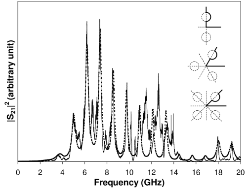
Figure 1: Transmission spectrum $S_{21}(k)$ of the 3-disk system in the fundamental domain with disk separation $R=20\sqrt{3}$ cm and radius $a=5$ cm. The dashed line is the semiclassical calculation. See [9] for details. (Insets) Geometry of the $n$-disk open billiard ($n=2,3,4$). The solid lines represent the fundamental domain in which the present experiments were carried out.

The spectral autocorrelation function was calculated as [9] $C(\kappa)=\left\langle|S_{21}(k-(\kappa/2))|^{2}|S_{21}(k+(\kappa/2))|^{2}\right\rangle_{k}$. The average is carried out over a band of wave vector centered at certain value $k_{0}$ and of width $\Delta k$. Since the transmission function is the superposition of many resonances, $|S_{21}(k)|^{2}=\sum_{i}c_{i}s_{i}^{\prime}/((k-s_{i})^{2}+s_{i}^{\prime 2})$, with $s_{i}+is_{i}^{\prime}$ the semiclassical resonances and $c_{i}$ the coupling which depend on the location of the probes, we have [15]

$$C(\kappa)=\pi\sum_{i,j}\frac{c_{i}c_{j}(s_{i}^{\prime}+s_{j}^{\prime})}{(\kappa-(s_{i}-s_{j}))^{2}+(s_{i}^{\prime}+s_{j}^{\prime})^{2}}.$$ (1)

In the case that there are no overlapping resonances, $|s_{i}-s_{j}|>>(s_{i}^{\prime}+s_{j}^{\prime})$, the small $\kappa$ behavior of the autocorrelation is $C(\kappa)\approx\pi\sum_{i}2c_{i}^{2}s_{i}^{\prime}/(\kappa^{2}+4s_{i}^{\prime 2})$. According to semiclassical theory, the above sum can be replaced by a single Lorentzian [16, 17, 18, 19]

$$C(\kappa)=C(0){\frac{1}{1+(\kappa/\gamma)^{2}}},$$ (2)

where $\gamma=\gamma_{cl}$, the classical escape rate with the velocity scaled to 1. The above equation was used to fit the spectral autocorrelation for small $\kappa$ and thus obtain the value of the experimental escape rate $\gamma_{qm}$ [8, 9]. Good agreement of the escape rate is obtained between $\gamma_{qm}$ obtained from the experiments and $\gamma_{cl}$ of the classical theory [9].

For intermediate $\kappa$, the semiclassical prediction of Eq. (2) fails because of the presence of the periodic orbits, which leads to non-universal behavior. Non-universal contributions can play in general a crucial role in determining the overall structure of the spectral autocorrelation, since they can be of the same order of the universal result of Random Matrix Theory. Recently, Agam [20] derived a semiclassical theory to build the connection between the nonuniversality of the spectral autocorrelation and the classical RP resonances. Consider the quantum mechanical propagator [21]

$$K({\vec{r}}_{1},{\vec{r}}_{2},t)=\frac{1}{2\pi\hbar i}\int G({\vec{r}}_{1},{\vec{r}}_{2},\sqrt{2m\varepsilon/\hbar^{2}})e^{-i\varepsilon t/\hbar}d\varepsilon,$$ (3)

with $\varepsilon=\hbar^{2}k^{2}/2m$. The integration is performed around $\varepsilon_{0}=\hbar^{2}k_{0}^{2}/2m$, with $\Delta\varepsilon=\hbar\upsilon\Delta k$ and $\upsilon=\hbar k_{0}/m$ is the group velocity of the classical particle. The integration in the $\varepsilon$ space can be changed into that in the $k$ space as $K({\vec{r}}_{1},{\vec{r}}_{2},t)=(\upsilon/2\pi i)e^{-i\varepsilon_{0}t/\hbar}\int_{\Delta k}G({\vec{r}}_{1},{\vec{r}}_{2},k_{0}+k)e^{-i\upsilon kt}dk$. The particle density is $\rho(t)=\left|K({\vec{r}}_{1},{\vec{r}}_{2},t)\right|^{2}$. The autocorrelation of the particle density is $C_{\rho}(\tau)=\left\langle\rho(t)\rho(t+\tau)\right\rangle_{t}-\left\langle\rho\right\rangle_{t}^{2}$ with $\left\langle\rho\right\rangle_{t}\equiv\lim_{t\to\infty}(1/T)\int_{0}^{T}\rho(t)dt$. Using the diagonal approximation, we get $C_{\rho}(\tau)=(\Delta k\upsilon^{2}/4\pi^{2}V^{2})\int d\kappa C(\kappa)e^{-i\upsilon\kappa\tau}$. Here $V$ is the volume of the system with $V\to\infty$ for open system. If one assumes that the above correlation is classical, one has [22, 23] $C_{\rho}(\tau)=\sum_{i=1}^{\infty}2b_{i}e^{-\gamma_{i}\upsilon\tau}\cos\gamma_{i}^{\prime}\upsilon\tau$, where the $c_{i}$ are the coupling coefficients, $\gamma_{i}\pm i\gamma_{i}^{\prime}$ the RP resonances of the corresponding classical system in wave vector space. Taking the Fourier transform of the above expression $\int d\tau C_{\rho}(\tau)e^{i\kappa\upsilon\tau}$, we get

$$C(\kappa)=\sum_{\pm,i=1}^{\infty}\frac{b_{i}^{\prime}\gamma_{i}}{\gamma_{i}^{2}+(\kappa\pm\gamma_{i}^{\prime})^{2}}.$$ (4)

with $b_{i}^{\prime}=2\pi V^{2}b_{i}/\Delta k\upsilon^{3}$.

We now turn to the classical dynamics of the system. The classical evolution is described by the Perron-Frobenius operator whose spectrum, known as the RP resonances, can be calculated as the poles of the classical Ruelle $\zeta$-function. For the hard disk system, the classical Ruelle $\zeta$ -function is [24]

$$\zeta_{\beta}(s)=\prod_{p}\,\left[1-\exp(sL_{p})/|\Lambda_{p}|\Lambda_{p}^{\beta-1}\right]^{-1},$$ (5)

here, $L_{p}$ the length of the periodic orbit $p$, $\Lambda_{p}$ the eigenvalue of the monodromy matrix associated with the periodic orbits. The $\zeta$ -function is analytical in the half-plane ${\rm Re}\>s<-P(\beta)$, and has poles in the other half-plane. In particular, $\zeta_{\beta}(s)$ has a simple pole at $s=-P(\beta)$. Here, $P(\beta)$ is the so-called Ruelle topological pressure, from which all the characteristic quantities of classical dynamics can be derived in principle. The classical escape rate is $\gamma_{cl}=-P(1)$. The poles of $\zeta_{\beta}(s)$ with $\beta=1$ are calculated since they contribute to the RP resonances with the sharpest width.

For the integrable $2$-disk system in the fundamental domain, there is just one prime periodic orbit. We have $\zeta_{1}(s)=1-t_{0}$, where $t_{0}=\exp[s(R-2a)]/\Lambda$, and $\Lambda=(\sigma-1)+\sqrt{\sigma(\sigma-2)}$, with the disk separation ratio $\sigma\equiv R/a$. The classical scattering resonances are $s_{n}=(\ln\Lambda\pm i2n\,\pi)/(R-2a\,)$, with $n=1,2,\cdots\,$. The classical escape rate is $\gamma_{cl}=(\,\ln\,\Lambda\,)/(R-2a)\,.$ The semiclassical resonances in the fundamental domain are [26] $(2n\pi+i(1/2)\ln\Lambda)/(R-2a)$ with $n=1,2,\cdots$. Substituting the semiclassical resonances into Eq.(1), one may express the full two-point correlation function as

$$C(\kappa)\propto\sum_{n=-\infty}^{\infty}\frac{b_{n}}{\gamma^{2}+(\kappa+n\gamma^{\prime})^{2}},$$ (6)

where $\gamma=\gamma_{cl}$, $\gamma^{\prime}=2\pi/(R-2a)$. On the other hand, since the RP resonances of the system are $(\ln\Lambda+i2n\pi)/(R-2a)$, if one puts these resonances into Eq. (4), the above expression (6) follows immediately. The experimental RP resonances are obtained from the autocorrelation by fitting it with Eq. (6). Since the transmission coefficient $S_{21}(f)$ and also the couplings $c_{i}$ of the quantum resonances depend on the location of the two probes, so does the coupling $b_{n}$ of the classical RP resonances. The comparison between experiment and theory is shown as Fig. 2 (left).

   

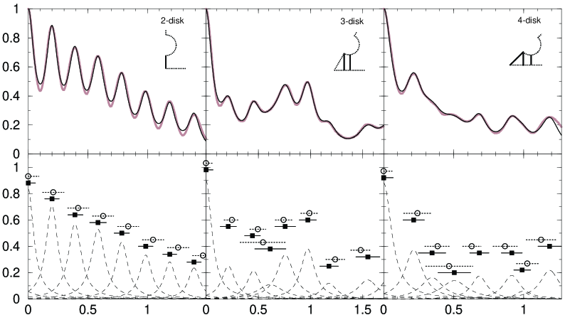
Figure 2: Autocorrelation function $C(\kappa)$ vs $\kappa$ (cm^-1) and Ruelle-Pollicott resonances of the $n$-disk system in the fundamental domain. (left). 2-disk system with $R=40$ cm and $a=5$ cm. (center). 3-disk system with $R/a=4\sqrt{3}$ and $a=5$ cm. (right). 4-disk system with $R/a=4\sqrt{2}$ and $a=5$ cm. (top). The gray line is the experimental autocorrelation. The solid line is the numerical fit to Eq. (4). (bottom). The dashed lines are the decomposition of the experimental $C(\kappa)$ into Lorentzians. The filled squares are the position $\gamma_{j}$ and the bars the widths $\gamma_{j}^{\prime}$ of the experimental RP resonances obtained from the decomposition. The open circles with dotted bars are the positions $\gamma_{j}$ and width $\gamma_{j}^{\prime}$ of the predicted RP resonances calculated from Eq. (5). The insets in the top panels show the leading periodic orbits (solid lines) for the different geometries.

For the chaotic $n$-disk system, making use of the cycle expansion [25] and also the symmetry factorization of the classical Ruelle $\zeta$-function, the RP resonances can be calculated very accurately [24]. For the $3$-disk system in the fundamental domain, the classical RP resonances are calculated by using 8 prime periodic orbits up to period 4. The calculation is very accurate for ${\rm Re}\>s<0.8$ [24]. The classical RP resonances can also be obtained experimentally by fitting the autocorrelation with Eq. (4). Because of the finite range of the experiment spectrum, only the first 8 or 9 RP resonances with small real part were obtained. The experimental autocorrelation with the theoretical prediction are shown as Fig. 2 (center).

For the $4$-disk system in the fundamental domain, the classical RP resonances are calculated by using 14 prime periodic orbits up to period 3. The experimental autocorrelation with the theoretical prediction are shown as Fig. 2 (right).

The agreement between the experimental RP resonances and the theoretical ones for the 2-disk sytem is 6% for the positions $\gamma_{j}$ and better than 30% for the widths $\gamma_{j}^{\prime}$, is 7% for $\gamma_{j}$ and 11% for $\gamma_{j}^{\prime}$ for the 3-disk sytem, and is 8% for $\gamma_{j}$ and 17% for $\gamma_{j}$ for the 4-disk sytem. We note that these agreements, in particular the wave-vector locations $\gamma_{j}$ should be considered as very good. The principal sources for the residual discrepancies are the nonideality of the absorbers, small symmetry-breaking perturbations and the suppression of some resonances at the neighborhood where the antennas are coupled which affects the autocorrelation function, therefore the position and the widths of RP resonances. Also very broad resonances are difficult to identify and can lead to an apparent enhancement of the observed widths, which can possibly account for the systematically larger widths that are observed.

Our investigation clearly demonstrates that the whole spectral autocorrelation can be understood completely in terms of the classical RP resonances. The meaning of these RP resonances in the classical context can be understood as follows. If one shoots particles toward the hard disk scatterer, the number of particles that will remain in the scattering region will decay as $N(t)=\sum_{i}a_{i}e^{-\alpha_{i}t}.$ Besides the general exponential decay at $\alpha_{0}=\upsilon\gamma_{cl}$, there are oscillations due to the fact that the RP resonances $\alpha_{i}=\upsilon(\gamma_{i}\pm i\gamma^{\prime}_{i})$ are not always real [24] as contrasted with the purely diffusive system. Taking the Fourier transform of $N(t)$, one can identify the Lorentzians in the spectrum with the RP resonances. Our work demonstrates that suitable quantum correlations diffuse just like classical observables in an open system.

It is remarkable that the same experiment yields both the quantum resonances and the classical RP resonances. Thus we have demonstrated experimentally the profound connection between quantum properties and classical diffusion. This connection is best seen in open quantum systems. While we have studied the model n-disk geometry, the results have broad implications for arbitrary chaotic geometries. The results of this work also have wider implications in a variety of phenomena in different fields in physics, such as photodissociation of atoms [27], nuclear decay [28], electronic transport, fluid dynamics, and acoustic and electromagnetic propagation.

We thank P. Pradhan for useful discussions. This work was supported by NSF-PHY-9722681.

^a electronic address : srinivas@neu.edu.

References

- [1] O. Bohigas, in: Chaos and Quantum Physics, edited by M.-J. Giannoni, A. Voros, and J. Zinn-Justin (Elsevier Science, New York, 1990), and references therein.
- [2] M. C. Gutzwiller, Chaos in Classical and Quantum Mechanics (Springer, New York, 1990).
- [3] E. J. Heller, Phys. Rev. Lett. 53, 1515(1984).
- [4] D. Ruelle, Phys. Rev. Lett. 56, 405 (1986); J. Stat. Phys. 44, 281 (1986).
- [5] M. Pollicot, Ann. Math. 131, 331 (1990).
- [6] K. B. Efetov, Adv. Phys. 32, 53(1983); K. B. Efetov, Supersymmetry in Disorder and Chaos (Cambridge University press, 1997).
- [7] (a) P. Gaspard, Chaos, Scattering and Statistical Mechanics (Cambridge University press, Cambridge, 1998). (b) P. Gaspard, Chaos 3, 427 (1993).
- [8] W. Lu, M. Rose, K. Pance, and S. Sridhar, Phys. Rev. Lett. 82, 5233 (1999).
- [9] W. Lu, L. Viola, K. Pance, M. Rose, and S. Sridhar, to appear in Phys. Rev. E (2000).
- [10] P. Cvitanović and B. Eckhardt, Nonlinearity 6, 277 (1993); P. Cvitanović, R. Artuso, R. Mainieri, and G. Vattay, Classical and Quantum Chaos: a Cyclist Treatise (unpublished, 1998).
- [11] P. Gaspard and S. A. Rice, J. Chem. Phys. 90, 2225 (1989); 90, 2242 (1989); 90, 2255 (1989); 91, E3279 (1989).
- [12] P. Gaspard, D. Alonso, T. Okuda, and K. Nakamura, Phys. Rev. E 50, 2591 (1994).
- [13] S. Sridhar, Phys. Rev. Lett. 67, 785 (1991).
- [14] (a) J. Stein, H.-J. Stöckmann, and U. Stoffregen, Phys. Rev. Lett., 75, 53 (1995), (b) H. Alt, et. al., Phys. Rev. Lett., 74, 62 (1995), (c) L. Sirko, P. M. Koch and R. Blümel, Phys. Rev. Lett., 78, 2940 (1997). (d) J. Hersch, M. R. Haggerty, and E. J. Heller, Phys. Rev. Lett. 83, 5342 (1999).
- [15] B. Eckhardt, Chaos 3, 613 (1993).
- [16] R. Blümel and U. Smilansky, Phys. Rev. Lett. 60, 477 (1988).
- [17] R. A. Jalabert, H. U. Baranger, and A. D. Stone, Phys. Rev. Lett. 65, 2442 (1990).
- [18] C. H. Lewenkopf and H. A. Weidenmüller, Ann. Phys. 212, 53 (1991).
- [19] Y.-C. Lai, R. Blümel, E. Ott and C. Grebogi, Phys. Rev. Lett. 68, 3491 (1992)
- [20] O. Agam, Phys. Rev. E 61, 1285 (2000).
- [21] S. Tomsovic and E. J. Heller, Phys. Rev. Lett. 67, 664 (1991); Phys. Rev. E 47, 282 (1993).
- [22] D. Ruelle, Thermodynamics formalism, Encyclopedia of Mathematics, Vol. 5 (Addison-Wesley, Reading, MA, 1978).
- [23] F. Christiansen, G. Paladin, and H. H. Rugh, Phys. Rev. Lett. 65, 2087 (1990).
- [24] P. Gaspard and D. Alonso Ramirez, Phys. Rev. A 45 , 8383 (1992).
- [25] P. Cvitanović and B. Eckhardt, Phys. Rev. Lett. 63, 823 (1989).
- [26] A. Wirzba, Chaos 2, 77 (1992).
- [27] O. Agam, Phys. Rev. A 60, R2633 (1999).
- [28] W. Bauer and G. F. Bertsch, Phys. Rev. Lett., 65, 2213 (1990).