Localized structures in coupled Ginzburg–Landau equations

Abstract

Coupled Complex Ginzburg-Landau equations describe generic features of the dynamics of coupled fields when they are close to a Hopf bifurcation leading to nonlinear oscillations. We study numerically this set of equations and find, within a particular range of parameters, the presence of uniformly propagating localized objects behaving as coherent structures. Some of these localized objects are interpreted in terms of exact analytical solutions.

1 Introduction

When an extended system is close to a Hopf bifurcation leading to uniform oscillations, the amplitude of the oscillations can be generically described in terms of the complex Ginzburg-Landau (CGL) equation [3]. When there are two fields becoming unstable at the same bifurcation, coupled complex Ginzburg-Landau equations (CCGL) should be used instead. This model set of equations appears in a number of contexts including convection in binary mixtures and transverse instabilities in unpolarized lasers [3, 4, 5].

Coherent structures such as fronts, shocks, pulses, and other localized objects play an important role in the dynamics of extended systems [6]. In particular, for the complex Ginzburg-Landau equation, they provide the building blocks from which some kinds of spatiotemporally chaotic behavior are built-up [7]. A systematic study of localized structures in CCGL equations in one spatial dimension was initiated in [8].

Here we present results on one dimensional CCGL equations in parameter ranges such that they can be written as

$$\partial_{t}A_{\pm}=\mu A_{\pm}+(1+i\alpha)\partial_{x}^{2}A_{\pm}-(1+i\beta)\left(|A_{\pm}|^{2}+\gamma|A_{\mp}|^{2}\right)A_{\pm}\>.$$ (1)

Group velocity terms of the form $\pm v_{g}\partial_{x}A_{\pm}$ are explicitly excluded, and $\gamma$ is restricted to take real values (without additional loss of generality, $\alpha$ and $\beta$ are also real parameters). In addition we just consider $1+\alpha\beta>0$ (Benjamin-Feir stable range). These restrictions are the appropriate ones for the description of transverse laser instabilities [4]. In that case $A_{\pm}$ are related to the two orthogonal circularly polarized light components. We further restrict our study to the case $0<\gamma<1$ which is the range obtained when atomic properties in the laser medium favor linearly polarized emission. In terms of the wave amplitudes $A_{\pm}$, wave coexistence is preferred.

2 Numerical studies

Many experiments on traveling wave systems or numerical simulations of Ginzburg–Landau–type equations [3, 9, 10] exhibit local structures that have a shape essentially time–independent and propagate with a constant velocity, at least during an interval of time where they appear to be coherent structures [11, 9, 8]. In order to analyze these structures it is common to reduce the initial partial differential equation to a set of ordinary differential equations by restricting the class of solutions to uniformly traveling ones. Localized structures are homoclinic or heteroclinic orbits in this reduced dynamical system, that is they approach simple solutions (typically plane waves) in opposite parts of the system, whereas they exhibit a distinct shape in between.

Instead of looking for solutions of the reduced dynamical system, we prefer here to resort to direct numerical solution of (1) under different initial conditions. A pseudo–spectral code [9, 12] with periodic boundary conditions and a second–order accuracy in time is used. Spatial resolution was typically 512 modes. Time step was typically $0.05$. The system size was always taken to be $L=512$. Several kinds of localized objects which maintain coherence for a time appear and travel around the system. Different initial conditions give birth to different kinds of structures. Some of them decay shortly, and the qualitative dynamics at long times becomes determined by the remaining ones, and essentially independent of the initial conditions.

The upper part of Fig. 1 shows the spatiotemporal evolution of $|A_{+}(x,t)|$ and $|A_{-}(x,t)|$ at parameter values $\alpha=-0.35\,,\,\beta=-2.0\mbox{ and }\gamma=0.2$. Time runs upwards and $x$ is represented in the horizontal direction. Lighter grey corresponds to the maximum values of $|A_{\pm}(x,t)|$ and darker to the minima.

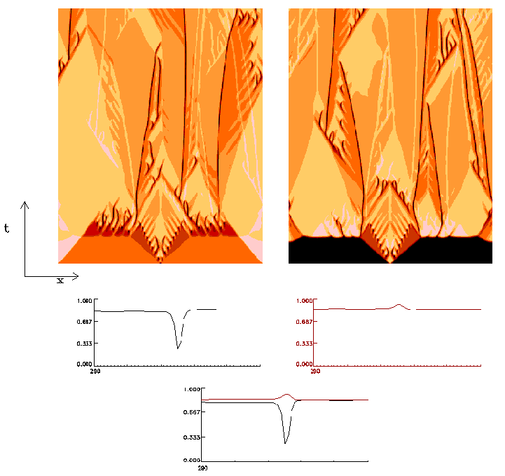
Figure 1: Upper panels: Spatiotemporal evolution of $|A_{+}(x,t)|$ and $|A_{-}(x,t)|$ with time running upwards from $t=0$ to $400$ and $x$ in the horizontal direction, from $x=0$ to $x=512$. Lighter grey corresponds to the maximum value of $|A_{\pm}(x,t)|$ and darker to the minimum. Parameter values are $\alpha=-0.35$, $\beta=-2.0$, and $\gamma=0.2$. Lower panels: A coupled hole–maximum pair at $t=399$ close to $x\approx 300$. This is the dominant coherent structure at long times. Left $|A_{+}(x,t)|$, right $|A_{-}(x,t)|$, and both graphs are superposed in the central bottom panel.

This particular evolution was obtained starting from $A_{+}(x,0)$ equal to the Nozaki-Bekki hole, a known analytical solution of the single Ginzburg-Landau equation [13, 14], and for $A_{-}(x,0)$ a Nozaki-Bekki pulse [14]. These are not exact solutions of the set of equations (1) so that this initial condition decays and gives rise to complex spatiotemporal structures. After a transient that will be described below, the configuration of the system consists in portions with a modulus nearly constant (corresponding to plane wave states) interrupted by localized objects with particle-like behavior. Dark features in $|A_{+}|$ appear where $|A_{-}|$ has bright features, thus indicating that the localized object carries a kind of anticorrelation between the fields. The lower panels of Fig. 1 show the modulus of the two fields at $t=399$ and $x\approx 300$, where one of such objects is present. One of the components shows a maximum in the modulus, whereas the other displays a deep minimum. We can call this object a “hole–maximum pair”. It seems to be a dissipative analog of the ‘out-gap’ solitons appearing in Kerr media with a grating [15], and here it is the characteristic object building-up the disordered intermittent dynamics seen at long times. It is clear that these objects connect the plane wave states (that is the constant modulus regions) filling most of the system. Before reaching the asymptotic state just described, the system evolves through configurations where additional kinds of localized objects are seen. The presence of the Nozaki-Bekki hole-pulse pair as initial condition in the central part of Fig. 1 gives birth to a pair of fronts which replace the initial lateral plane-waves by new ones. Interestingly, a different kind of localized object is seen to form just where the initial hole-pulse pair was placed. A close-up of it at $t=90$ is displayed in Fig. 2. It is a kind of coupled maximum-maximum pair. The moduli of the two fields are superposed in the central panel showing the full object. The lateral small bumps are propagating waves that travel towards the central maxima. Thus the center of the coherent structure acts as a wave sink [11].

Figure 2: Snapshots of part of the system in Fig. 1 at $t=90$ showing a localized maximum–maximum wave sink.

In Figure 3 the spatiotemporal evolution of $|A_{+}(x,t)|$ and $|A_{-}(x,t)|$ was obtained using as initial conditions a sharp phase jump at the center of the system, with small random white noise added. The parameter values are $\alpha=0.6\,,\,\beta=-1.4\mbox{ and }\gamma=0.7$. After a short time, the system reaches a state dominated by branching hole–hole pair structures. Lighter grey correspond to the maximum values of $|A_{\pm}(x,t)|$ and darker to the minima. The two big triangles correspond to regions of constant modulus, that is, plane waves. The bottom panels show $|A_{+}|$ and $|A_{-}|$ in a portion of the system at these early times. Both are superposed in the central panel to show the complete matching of the two fields.

At longer times, all the hole-hole pairs disappear from the system, thus indicating that they are not stable objects at this value of the parameters. The system decays to the same state as at the end of Fig. 1: the dominant coherent structures are the maximum-hole pairs.

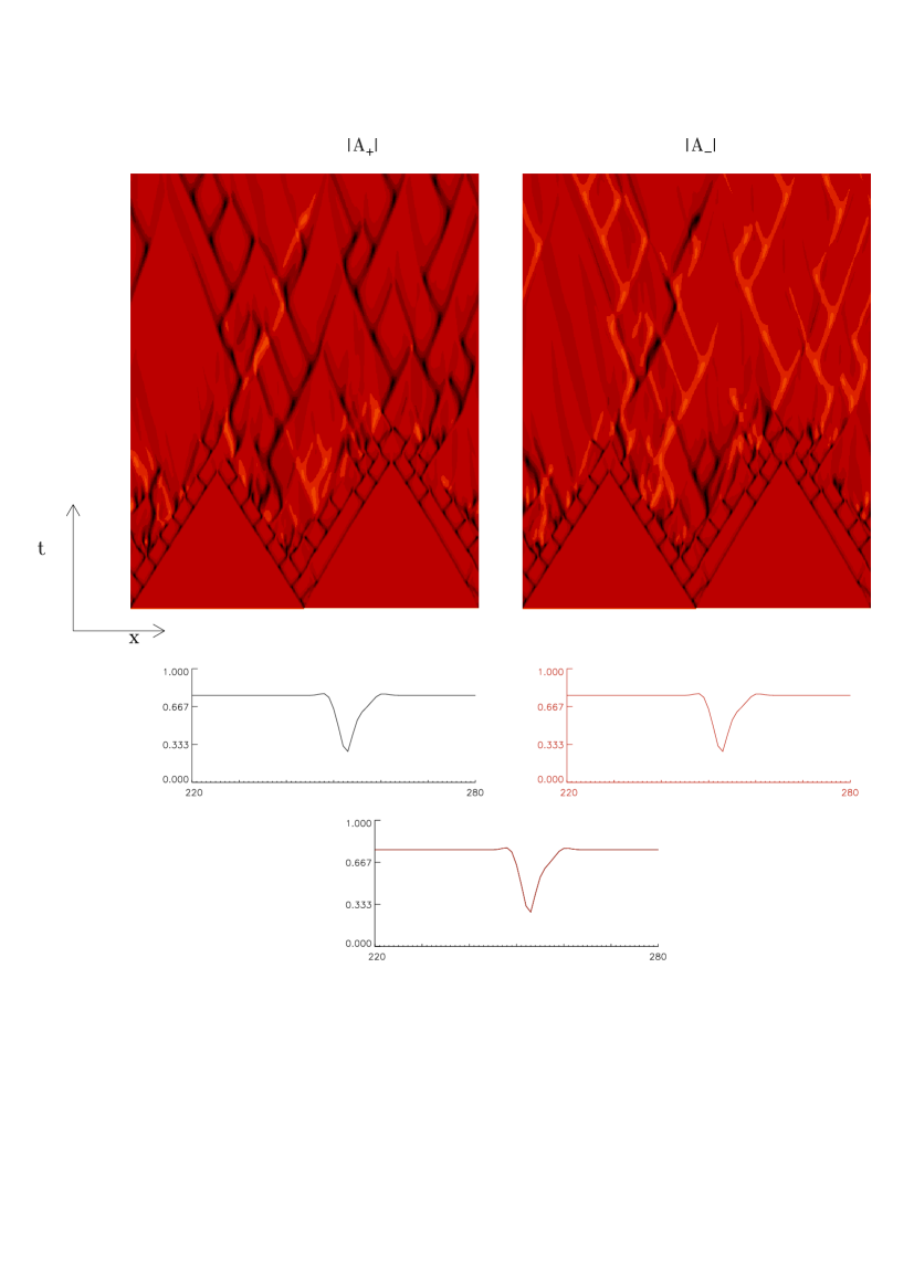
Figure 3: Spatiotemporal evolution of $|A_{+}(x,t)|$ and $|A_{-}(x,t)|$ with time running upwards from $0$ to $400$ and $x$ in the horizontal direction from $0$ to $512$. Lighter red correspond to the maximum value of $|A_{\pm}(x,t)|$ and darker to the minimum. Bottom panels (left and right) show one of the localized hole-hole objects dominating the early dynamics. Central bottom panel superpose them, showing its perfect matching. Both fields, then, have exactly the same modulus around the core of the coherent structure, as in the ansatz (2).

3 Exact solutions

The different spatiotemporal evolutions shown in the previous figures (1)–(3) are themselves interesting enough for a detailed study. The localized objects appearing in the simulations are clearly responsible for most of the complex dynamics in the system. We can interpret some of the observed structures from a simple ansatz:

$$A_{+}(x,t)=e^{i\varphi}A_{-}(x,t)$$ (2)

where $\varphi$ is constant, and $A_{-}(x,t)$ is any solution of the single CGL equation:

$$\partial_{t}A_{-}=A_{-}+b\,\partial_{x}^{2}A_{-}-c\mid A_{-}\mid^{2}A_{-}\>,$$ (3)

where $b=1+i\alpha$ and $c=(1+\gamma)+i(1+\gamma)\beta$ .

This simple ansatz gives us a rather rich set of exact solutions: for each known analytical solution of the single CGL equation (3), there is a corresponding solution of the CCGL equation set, in which $A_{-}$ and $A_{+}$ have essentially the same shape except for a constant global phase. In particular, hole, pulse, shock, and front solutions are localized solutions analytically known for the single equation [13, 14, 11, 16], so that hole-hole, pulse-pulse, shock-shock and front-front pairs are immediately found as analytical solutions of the CCGL set. In particular pulse-pulse and hole-hole structures are present in Figs. 1 to 3, and turn out to be well described by the ansatz (2).

It is worthwhile to note that the studies of instability for these objects in the complex Ginzburg-Landau equation are immediately translated into instability results for the paired structures in CCGL equations.

4 Conclusion

In summary, we have shown numerically the existence of different kinds of localized objects, responsible for the complex behavior or solutions of the CCGL equations. Some of these objects can be understood in terms of exact solutions arising from a simple ansatz. A more detailed analysis is still needed, however. In particular, the hole-maximum structure, which appears as the dominant coherent structure at long times, can not be described by our ansatz. In addition, much more work is needed in order to establish the stability properties of the different objects, and the nature of their interactions. In a recent work[17, 18] new exact solutions of equation 1 were obtained by using the Painlevé expansion method. The authors describe these solutions as analogues of the Nozaki-Bekki solutions [13, 14]. Comparison of these solutions, different from the ansatz (2), with our numerical results is under progress.

Financial support from DGICYT Projects PB94-1167 and PB97-141-C02-01 is acknowledged. R.M. Acknowledge financial support from CONICYT-Fondo Clemente Estable (Uruguay)

References

- [1] Raúl Montagne. E–mail: montagne@fisica.edu.uy.
- [2] Emilio Hernández-García. E–mail: emilio@imedea.uib.es.
- [3] M. C. Cross and P. C. Hohenberg. Rev. Mod. Phys., 65 (1993) 851 and references therein.
- [4] M. San Miguel. Phys. Rev. Lett., 75 (1995) 425.
- [5] L. Gil. Phys. Rev. Lett., 70 (1993) 162.
- [6] H. Riecke. Localized structures in pattern-forming systems. in Pattern formation in continuous and coupled systems : a survey volume, ed. by Martin Golubitsky, Dan Luss, and Steven H. Strogatz, Springer (New York, 1999). patt-sol/9810002
- [7] M. van Hecke. Phys. Rev. Lett., 80 (1998) 1896. chao-dyn/9707010
- [8] M. van Hecke, C. Storm, and W. van Saarloos. Physica D, 134 (1999) 1. patt-sol/9902005
- [9] R. Montagne, E. Hernández-García, A. Amengual, and M. San Miguel. Phys. Rev. E, 56 (1997) 151. chao-dyn/9701023
- [10] E. Hernández-García, M. Hoyuelos, R. Montagne, Maxi San Miguel, and Pere Colet. Int. J. Bifurcation and Chaos, 9 (1999) 2257. chao-dyn/9902018
- [11] W. van Saarloos and P. C. Hohenberg. Physica D, 56 (1992) 303, and (Errata) Physica D 69 (1993) 209.
- [12] M. Hoyuelos, E. Hernández-García, P. Colet, and M. San Miguel. Comp. Phys. Comm., 121–122 (1999) 414. chao-dyn/9903011
- [13] K. Nozaki and N. Bekki. Phys. Rev. Lett., 51 (1983) 2171.
- [14] K. Nozaki and N. Bekki. J. Phys. Soc. Japan, 53 (1984) 1581.
- [15] J. Feng and F. K. Kneubühl. IEEE J. Quantum Electron., 29 (1993) 590.
- [16] R. Conte and M. Musette. Physica D, 69 (1993) 1.
- [17] R. Conte and M. Musette. Analytic expressions of hydrothermal waves, in XXXI-th Symposium on Mathematical physics, Torún, 18-21 May, 1999, to appear in Reports on Mathematical Physics (2000).
- [18] R. Conte and M. Musette. On the solitary wave of two coupled nonintegrable Ginzburg-Landau equations, in Nonlinear integrability and all that: twenty years after NEEDS’79, ed. by M. Boiti, L. Martina, F. Pempinelli, B. Prinari, and G. Soliani, World Scientific (Singapore, 2000).