Dynamics of One- and Two-dimensional Kinks in Bistable Reaction-Diffusion Equations with Quasi-Discrete Sources of Reaction

Abstract

We study the evolution of fronts in a bistable reaction-diffusion system when the nonlinear reaction term is spatially non-homogeneous. This equation has been used to model wave propagation in various biological systems. Extending previous works on homogeneous reaction terms, we derive asymptotically an equation governing the front motion, which is strongly nonlinear and, for the two-dimensional case, generalizes the classical mean curvature flow equation. We study the motion of one- and two- dimensional fronts, finding that the non-homogeneity acts as a ”potential function” for the motion of the front; i.e., there is wave propagation failure and the steady state solution depends on the structure of the function describing the non-homogeneity.

1 Introduction

In this paper we consider the following equation

$$\phi_{t}=D\ \Delta\phi+\alpha\ \beta(x,y)\ [f(\phi)+h],$$ (1)

in a bounded region, $\Omega\subset R^{n}$, $n=1,2$, with smooth boundary $\partial\Omega$ for Neumann boundary conditions on $\partial\Omega$. The positive constants $D$ and $\alpha$ are the diffusion coefficient and the production rate of the reactants, respectively. The function $f$ is a bistable function (the derivative of a double well potential); i.e., a real odd function with positive maximum equal to $\phi^{\ast}$, negative minimum equal to $-\phi^{\ast}$ and precisely three zeros in the closed interval $[a_{-},a_{+}]$ located at $a_{-}$, $a_{0}$ and $a_{+}$. For simplicity and without lost of generality we will consider in our analysis $a_{-}=-1$, $a_{0}=0$ and $a_{+}=1$. The prototype example is $f(\phi)=(\phi-\phi^{3})/2$. The constant $h$ in (1), assumed to be small in absolute value, specifies the difference of the potential minima of the system as will be explained later. Altough the analysis presented below will be valid for a general class of positive differentiable function $\beta$, we have in mind some particular cases which are described below. In what follows $\eta$ is a positive constant.

Case 1) There is a sequence of points on the real line, $x_{k}$, $k=1,\ldots,N$, with $N$ finite or infinite, where the function $\beta$ reaches a maximum,

$$\beta(x)=\sum_{k=1}^{N}\ e^{-\eta(x-x_{k})^{2}}.$$ (2)

Case 2) There is a sequence of lines in the plane, $y_{k}$, $k=1,\ldots,N$, with $N$ finite or infinite, where the function $\beta$, independent of $x$, reaches a maximum,

$$\beta(x,y)=\sum_{k=1}^{N}\ e^{-\eta(y-y_{k})^{2}}.$$ (3)

Case 3) There is a sequence of points in the plane, $(x_{k},y_{j})$, $k=1,\ldots,N$, $j=1,\ldots,M$ with $N$ and $M$ finite or infinite, where the function $\beta$ reaches a maximum,

$$\beta(x,y)=\sum_{k=1}^{N}\sum_{j=1}^{M}\sigma(x-x_{k},y-y_{j};\eta),\ \ \ \ \ \ \ \ \ \ {\mbox{w}here}\ \ \ \ \ \ \ \ \ \ \sigma(x,y;\eta)=e^{-\eta(x^{2}+y^{2})}.$$ (4)

Case 4) There is a sequence of circles in the plane, $\rho=\rho_{k}$, $k=1,\ldots,N$, with $N$ finite or infinite, and where $\rho$ represents the radial polar coordinate, where the function $\beta$ reaches a maximum,

$$\beta(\rho)=\beta(x,y)=\sum_{k=1}^{N}\ e^{-\eta(\rho-\rho_{k})^{2}}.$$ (5)

For sufficiently large values of $\eta$, $\beta$ as given by (2-5) are approximations of distributions of discrete sources of reaction. We will refer to the points $x_{k}$ and $(x_{k},y_{j})$,$k=1,\ldots,N$, $j=1,\ldots,M$ as quasi-discrete sources of reaction or quasi-discrete (QD) sites and to the stripes $y=y_{k}$ and circles $\rho=\rho_{k}$ $k=1,\ldots,N$ as quasi-semi-discretes sources of reaction or quasi-semi-discrete (QS) sites. We define $d$ to be the shortest distance between two adjacent QD or QS sites.

In the last several years, partial differential equations with nonlinear discrete sources of reaction (NDSR) have been used to model phenomena in different fields ranging from physics to biology, including the study of pinning in the dislocation motion in crystals, breathers in nonlinear crystal lattices, Josephson junction arrays and the biophysical description of calcium release waves [kn:flakla1]-[kn:kee2]. The non-homogeneous version of the bistable equation with discrete sources of reaction

$$\phi_{t}=D\ \Delta\phi+\alpha\ \sum_{k}\delta(x-x_{k})\ [f(\phi)+h],$$ (6)

has received special attention for its applicability to the dynamics of charge density waves [kn:fuklee1], [kn:cop1]-[kn:mitkla1], [kn:gru1, kn:gru2] and to the dynamics of calcium release waves [kn:mitkla1, kn:kee1, kn:kee2]. Equation (6) describes the evolution of some concentration (in chemical or biological applications) or order parameter (in some physical applications) $\phi$ in a discrete array of nonlinear reaction sites embedded in a continuum. In [kn:kee2] equation (1) with an additional term on the right side, $-a\ \phi$, and $\beta$ given by (2) has been used to model calcium release and uptake in cardiac cells via ryanodine receptors. In this model $\phi$ represents the concentration of $Ca^{2+}$ and $f(\phi)$ represents the calcium-induced calcium release (CICR) activity of the release mechanism. When $a=1$, the model allows for continuous spatial uptake, whereas when $a=0$, it is assumed that release and uptake both occur at the QD or QS sites. In [kn:mitkla2] the function $f(\phi)$ was taken to be the derivative of a sine-Gordon potential; i.e., $f(\phi)=-\sin(\phi)$. Note that this last function is equal to the derivative of a double well potential, as described above, in a restricted domain of definition.

When the function $\sum_{k}\delta(x-x_{k})$ in (6) is replaced by a constant, say $1$, then by appropriate rescaling we have the bistable equation

$$\phi_{t}=b\ \Delta\phi+f(\phi)+h,$$ (7)

which describes a phase transition dynamics process,where $\phi$ is a non-conserved order parameter. Note that for the particular cases $f(\phi)=(\phi-\phi^{3})\ /\ 2$ and $f(\phi)=sin(\phi)$ equation (7) is the Ginzburg-Landau equation and the overdamped sine-Gordon equation respectively. Equation (7) can be derived by considering a physical system whose free energy is assumed to be of the form

$$F_{b}(\phi)=\int_{\Omega}\left(\frac{b}{2}(\nabla\phi)^{2}+F(\phi)-h\,\phi\right)dx,$$ (8)

where $F$ is a double well potential having the two equal minima. Note that $F(\phi)-h\ \phi$ is a double-well potential with one local minimum and one global minimum. The functional derivative of (8) is given by

$$\frac{\delta F_{b}}{\delta\phi}=-b\ \Delta\phi-f(\phi)-h,$$ (9)

where $f(\phi)=-F^{\prime}(\phi)$. The right side of equation (9) may be considered as a generalized force indicative of the tendency of the free energy to decay towards a minimum. The bistable equation (7) is obtained by assuming that $\phi$ decreases at a rate proportional to that generalized force.

Equation (7) for $n=1$ possesses a travelling kink solution moving with velocity proportional to $h$. A kink is a solution that connects the two local minima of the double well potential. If $h\neq 0$ then the kink propagates from the locally stable minimum to the globally stable minimum. Of special interest are kinks in which the transition between the two minima takes place in a region of order of magnitude $\epsilon\ll 1$; i.e., the kinks have rapid spatial variation between the two ground states. For this case, the point on the line (for $n=1$) or the set of points in the plane (for $n=2$) for which the order parameter $\phi$ vanishes are called the interface or the front. Allen and Cahn [kn:allcah1] and Rubinstein, Sternberg and Keller [kn:rubste1] showed that for (7) with $b\ll 1$ and $h=0$ curved fronts in the plane move with normal velocity proportional to their curvature, according to the FMC (flow by mean curvature) equation

$$\frac{s_{t}}{(1+s_{x}^{2})^{\frac{1}{2}}}=\frac{s_{xx}}{(1+s_{x}^{2})^{\frac{3}{2}}}-\bar{h},$$ (10)

where $y=s(x,t)$ is the Cartesian description of the interface in the plane, and $\bar{h}$ is proportional to $h$ (see also [kn:fif1]). For a circular interface and $\bar{h}=0$ (both phases have equal potential), the curvature is the reciprocal of the radius $R$, and (10) becomes $R_{t}=-\frac{1}{R(t)}$, whose solution satisfying $R(0)=R_{0}$ is given by $R(t)=\sqrt{R_{0}^{2}-2t}$; i.e., circles shrink to a point at a critical time $t_{c,0}=\frac{R_{0}^{2}}{2}$. For $\bar{h}>0$ the value of the critical time decreases; i.e., $t_{c,\bar{h}}<t_{c,0}$. For $\bar{h}<0$ there exists a critical value $\bar{h}_{c}$ such that if $\bar{h}>\bar{h}_{c}$, then circles still shrink to a point in a finite time $t_{c,\bar{h}}<t_{c,0}$, whereas if $\bar{h}<\bar{h}_{c}$, then circles grow unboundedly. For more general shapes, such an expression for the distance of every point in the interface from the origin is difficult to obtain, but there are some analytical results showing that the behaviour is similar. Gage and Hamilton [kn:gagham1] proved that (10) shrinks convex curves embedded in the plane $R^{2}$ to a point. They showed that such curves remain convex and become asymptotically circular as they shrink. Grayson [kn:gra1] extended this result to a more general case showing that embedded curves become convex without developing singularities; i.e., curve shortening shrinks embedded plane curves smoothly to points, with round limiting shape.

On rescaling (6) $x\rightarrow x/d$ and $t\rightarrow\alpha\ t$ and defining $b=D/\alpha\ d^{2}$ (for n = 1 ) [kn:mit1], equation (6) becomes

$$\phi_{t}=b\ \Delta\phi+\sum_{k}\delta(x-x_{k})\ [f(\phi)+h].$$ (11)

The parameter $b$ can be thought of as a measure of how close (11) is to its continuous limit (7). If $b\rightarrow\infty$ equation (11) behaves like its continuous counterpart (with the corresponding rescaling); i.e., it possesses a travelling kink solution moving with velocity proportional to $h$ [kn:mit1]. For $b$ small, Mitkov et al. [kn:mitkla1, kn:mit1] have found numerically that the front dynamics results in burst waves characterized by time periodicity in a frame moving along with the front. For $b$ small enough, the wave no longer propagates, but relaxes to a stationary kink; i.e., the waves are pinned.

For the one-dimensional version of (1), with $\beta$ given by (2), as well as for the continuous spatial uptake version, $a=1$, Keener [kn:kee2] demonstrated the failure of wavefront propagation if the separation between QD sites is large enough.

For (1) we define the spatial and temporal dimensionless variables as in [kn:mit1]

$$\hat{x}=\frac{x}{d},\ \ \ \ \ \ \ \ \ \ \hat{y}=\frac{y}{d},\ \ \ \ \ \ \ \ \ \ \hat{t}=\alpha\ t,$$ (12)

and we also define the following dimensionless parameters

$$\epsilon=\frac{1}{d}\ \sqrt{\frac{D}{\alpha}},\ \ \ \ \ \ \ \ \ \ \ \ \hat{\eta}=\eta\ d^{2},\ \ \ \ \ \ \ \ \ \ \ \ \hat{h}=\frac{h}{\epsilon}.$$ (13)

Substituting (12) and (13) into (1), dropping the $\hat{}$ from the variables and parameters and further rescaling the time variable we obtain

$$\epsilon^{2}\ \phi_{t}=\epsilon^{2}\ \Delta\phi+\beta(x,y)\ [f(\phi)+\epsilon\ h],$$ (14)

We will consider the case $0<\epsilon\ll 1$; i.e., when diffusion is slow, $d$ is large or reaction is fast.

In Section 2 we make a formal asymptotic analysis to derive an equation of motion for the front in equation (14), which in Cartesian coordinates reads

$$s_{t}=\frac{s_{xx}}{1+s_{x}^{2}}+\frac{s_{x}\ \beta_{x}(x,s)}{2\ \beta(x,s)}-\frac{\beta_{y}(x,s)}{2\ \beta(x,s)}-\beta(x,s)^{\frac{1}{2}}\ \bar{h}$$ (15)

where the parameter $\bar{h}$, which is proportional to $h$, is defined later. Note that equation (15) expressed in polar coordinates reads

$$\rho_{t}=\frac{\rho_{\theta\theta}\ \rho-2\ \rho_{\theta}^{2}-\rho^{2}}{\rho\ (\rho^{2}+\rho_{\theta}^{2})}+\frac{\rho_{\theta}}{\rho^{2}}\ \frac{\beta_{\theta}(\rho,\theta)}{2\ \beta(\rho,\theta)}-\frac{\beta_{r}(\rho,\theta)}{2\ \beta(\rho,\theta)}-\beta(\rho,\theta)^{\frac{1}{2}}\ \bar{h}.$$ (16)

This equation generalizes the FMC equation (10) with a strong nonlinearity accounting for the influence of the function $\beta$ on the front motion. The method we use is the same as that used in [kn:rotnep1] for the study of the evolution of kinks in the nonlinear wave equation. We present it here in some detail for the sake of completeness. In Section 3 we study the evolution of one-dimensional fronts by means of (15). We show that for $\bar{h}=0$ the function $\beta$ acts as a ”potential function” for the motion of the front; i.e., a front initially placed between two maxima of $\beta$ asymptotically approaches the intervening minimum, unlike the classical homogeneous equation (7), for which fronts, whose motion is governed by (10), move with a velocity proportional to $\bar{h}$. This result is a consequence of the non-homogeneity of the nonlinear reaction term. In Section 4 we study the evolution of two-dimensional fronts by means of (15). We show analytically that a radially symmetric and non-constant function $\beta$ stabilizes a circular domain of one phase inside the other phase analogous to the one-dimensional case. This behavior, also arised as a consequence of the non-homogeneity of the nonlinear reaction term. The evolution of closed curves according to (15) for $\beta$ given by (4) is studied numerically. We observe that closed convex curves evolve to a final shape determined by $\beta$. Our conclusions appear in Section 5.

2 Asymptotic Analysis: Derivation of the Equation of Front Motion

We assume that for small $\epsilon\geq 0$ and all $t\in[0,T]$, the domain $\Omega$ can be divided into two open regions $\Omega_{+}(t;\epsilon)$ and $\Omega_{-}(t,\epsilon)$ by a curve $\Gamma(t;\epsilon)$, which does not intersect $\partial\Omega$. This interface, defined by

$$\Gamma(t;\epsilon):=\left\{x\in\Omega:\phi(x,t;\epsilon)=0\right\},$$ (17)

is assumed to be smooth, which implies that its curvature and its velocity are bounded independently of $\epsilon$. We also assume that there exists a solution $\phi(x,t;\epsilon)$ of (1), defined for small $\epsilon$, for all $x\in\Omega$ and for all $t\in[0,T]$ with an internal layer. As $\epsilon\rightarrow 0$ this solution is assumed to vary continuously through the interface, taken the value $1$ when $x\in\Omega_{+}(t;\epsilon)$, $-1$ when $x\in\Omega_{-}(t,\epsilon)$, and varying rapidly but smoothly through the interface. By carrying out a singular perturbation analysis for $\epsilon\ll 1$, we obtain the law of motion of the interface, treating it as a moving internal layer of width $O(\epsilon)$. We focus on the dynamics of the fully developed layer, and not on the process by which it was generated.

In Cartesian coordinates the interface is represented by $y=s(x,t,\epsilon)$ for $\epsilon$ sufficiently small. We assume that the curvature of of the front is small compared to its width and define, in a neighborhood of the interface, a new variable

$$z:=\frac{y-s(x,t,\epsilon)}{\epsilon}$$

which is ${\cal O}(1)$ as $\epsilon\rightarrow 0$. We call $\Phi$ the asymptotic form of $\phi$ as $\epsilon\rightarrow 0$ with $z$ fixed; i.e.,

$$\phi=\Phi(z,x,t,\epsilon).$$ (18)

The field equation (14) in $(z,x,t)$ coordinates becomes

$$\epsilon^{2}\ \Phi_{t}-\epsilon\ s_{t}\ \Phi_{z}=\epsilon^{2}\ \Phi_{xx}-2\ \epsilon\ s_{x}\ \Phi_{zx}+(1+s_{x}^{2})\Phi_{zz}-$$

$$-\epsilon\ s_{xx}\ \Phi_{z}+\beta(x,s+\epsilon\,z)\ f(\phi)+\epsilon\ \beta(x,s+\epsilon\,z)\ h.$$ (19)

The asymptotic expansions of $\Phi$ and $S$ are assumed to have the form

$$\Phi\sim\Phi^{0}+\epsilon\ \Phi^{1}+{\cal O}(\epsilon^{2}),\ \ \ \ \ {\mbox{a}s}\ \ \epsilon\rightarrow 0.$$

Thus

$$\beta(x,s+\epsilon\,z)=\beta(x,s)+\epsilon\ z\ \beta_{y}(x,s)+{\cal O}(\epsilon^{2}).$$

Substituting into (19) and equating coefficients of the corresponding powers of $\epsilon$ we obtain the following problems for ${\cal O}(1)$ and ${\cal O}(\epsilon)$ respectively:

$$(\ 1+s_{x}^{2}\ )\ \Phi_{zz}^{0}+\beta(x,s)\ f(\Phi^{0})=0,$$ (20)

$$(\ 1+s_{x}^{2}\ )\ \Phi_{zz}^{1}+\beta(x,s)\ f^{\prime}(\Phi^{0})\ \Phi^{1}=(s_{xx}-s_{t})\Phi_{z}^{0}+$$

$$+2\ s_{x}\ \Phi_{zx}^{0}-\beta_{y}(x,s)\ z\ f(\Phi^{0})-\beta(x,s)\ h.$$ (21)

In order to solve (20) we define a new variable

$$\xi:=\frac{\beta(x,s)^{\frac{1}{2}}}{(1+s_{x}^{2})^{\frac{1}{2}}}\ z.$$ (22)

In terms of $\xi$, equation (20) reads

$$\Phi_{\xi\xi}^{0}+f(\Phi^{0})=0,$$ (23)

whose solution is $\Phi^{0}=\Psi(\xi)$, the unique solution of $\ \ \Psi^{\prime\prime}+f(\Psi)=0,\ \Psi(\pm\infty)=\pm 1,\ \Psi(0)=0$. Thus

$$\Phi^{0}=\Phi^{0}\left(\frac{\beta(x,s)^{\frac{1}{2}}}{(1+s_{x}^{2})^{\frac{1}{2}}}\ z\right).$$ (24)

In terms of $\xi$, $x$ and $t$, equation (21) reads

$$\Phi_{\xi\xi}^{1}+f^{\prime}(\Phi^{0})\ \Phi^{1}=\frac{s_{xx}-s_{t}}{\beta(x,s)^{\frac{1}{2}}\ (1+s_{x}^{2})^{\frac{1}{2}}}\ \Phi_{z}^{0}+$$

$$+2\ s_{x}\ \left[\frac{\beta_{x}(x,s)+\beta_{y}(x,s)\ s_{x}}{2\ \beta(x,s)^{\frac{3}{2}}\ (1+s_{x}^{2})^{\frac{1}{2}}}-\frac{s_{x}\ s_{xx}}{\beta(x,s)^{\frac{1}{2}}\ (1+s_{x}^{2})^{\frac{3}{2}}}\right]\ (\xi\ \Phi_{\xi\xi}^{0}+\Phi_{\xi}^{0})$$

$$-\frac{\beta_{y}(x,s)\ (1+s_{x}^{2})^{\frac{1}{2}}}{\beta(x,s)^{\frac{3}{2}}}\ \xi\ f(\Phi^{0})-h.$$ (25)

It is straightforward to check that $\Psi^{\prime}(\xi)$ satisfies the homogeneous equation

$$\Phi_{\xi\xi}^{1}+f^{\prime}(\Phi^{0})\ \Phi^{1}=0.$$ (26)

That means that the operator $\Lambda$ defined as follows

$$\Lambda:=\frac{\partial^{2}}{\partial\xi^{2}}+f^{\prime}(\Phi^{0})$$ (27)

has a simple eigenvalue at the origin with $\Psi^{\prime}$ as the corresponding eigenfunction. Then the solvability condition for the equation (25) gives

$$\frac{s_{xx}-s_{t}}{\beta(x,s)^{\frac{1}{2}}\ (1+s_{x}^{2})^{\frac{1}{2}}}\ \int_{-\infty}^{\infty}(\Psi^{\prime})^{2}\ d\xi+$$

$$2\ s_{x}\ \left[\frac{\beta_{x}(x,s)+\beta_{y}(x,s)\ s_{x}}{2\ \beta(x,s)^{\frac{3}{2}}\ (1+s_{x}^{2})^{\frac{1}{2}}}-\frac{s_{x}\ s_{xx}}{\beta(x,s)^{\frac{1}{2}}\ (1+s_{x}^{2})^{\frac{3}{2}}}\right]\ \int_{-\infty}^{\infty}(\xi\ \Psi^{\prime\prime}+\Psi^{\prime})\ \Psi^{\prime}\ d\xi$$

$$-\frac{\beta_{y}(x,s)\ (1+s_{x}^{2})^{\frac{1}{2}}}{\beta(x,s)^{\frac{3}{2}}}\ \int_{-\infty}^{\infty}\xi\ f(\Psi)\ \Psi^{\prime}\ d\xi-h\int_{-\infty}^{\infty}\Psi^{\prime}\ d\xi=0.$$ (28)

A simple calculation shows that

$$\int_{-\infty}^{\infty}\xi\Psi^{\prime}\Psi^{\prime\prime}d\xi=-\frac{1}{2}\int_{-\infty}^{\infty}(\Psi^{\prime})^{2}d\xi\ \ \ \ \ \ \ \ \ \ \mbox{and}\ \ \ \ \ \ \ \ \ \ \int_{-\infty}^{\infty}\xi\ f(\Psi)\Psi^{\prime}\ d\xi=\frac{1}{2}\int_{-\infty}^{\infty}(\Psi^{\prime})^{2}d\xi\ \ \ \ \ \ \ \ \ \$$ (29)

We define

$$\bar{h}:=h\ \frac{\Psi(+\infty)-\Psi(-\infty)}{\int_{-\infty}^{\infty}(\Psi^{\prime})^{2}d\xi},$$ (30)

Substituting (29) and (30) into (28) and rearranging terms we get (15). Note that for $f(\phi)=\frac{\phi-\phi^{3}}{2}$ (Ginzburg-Landau theory), $\Psi(\xi)=\tanh\frac{\xi}{2}$ and $\bar{h}=3\ h$ whereas for $f(\phi)=\sin\phi$ (overdamped sine-Gordon), $\Psi(\xi)=4\ \mbox{tan}^{-1}e^{\xi}-\pi$ and $\bar{h}=\frac{\pi}{4}\ h$.

3 Front Motion in 1D

For a one-dimensional system, equation (15) reads

$$s_{t}=-\frac{\beta^{\prime}(s)}{2\ \beta(s)}-\beta^{\frac{1}{2}}(s)\ \bar{h}.$$ (31)

We will concentrate on functions $\beta$ of the form (2),

$$\beta(s)=\sum_{k=1}^{N}\ e^{-\eta(s-x_{k})^{2}},$$ (32)

altough the same analysis can be done for a general differentiable function.

In order to analyze the motion of the front we need to look at the roots of the function

$$g(s)=-\beta^{\prime}(s)-2\ \beta^{\frac{3}{2}}(s)\ \bar{h},$$ (33)

which are the equilibrium points of the interface. As an example, in Figure 1 we can see the graph of $\beta(s)$ and $g(s)$ respectively for $\eta=1000$ and $x_{1}=2$, $x_{2}=1$, $x_{3}=0$ and $x_{4}=-1$, $x_{5}=-2$ and various values of $\bar{h}$. For $\bar{h}=0$, $g(s)$ has $9$ roots in the range considered. Five of them are $x_{k}$, $k=1,\ldots,5$; i.e., they correspond to the maxima of $\beta(s)$. The other four correspond to the minima of $\beta(s)$: $s_{1}$, $s_{2}$, $s_{3}$ and $s_{4}$ from left to right. It is easy to see that $s_{k}$, $k=1,\ldots,4$ are stable whereas $x_{k}$, $k=1,\ldots,5$ are unstable. Thus one dimensional fronts initially at non-equilibrium points $x$ move until they reach a stable equilibrium point; i.e., a front initially at a point $x\in(x_{k},x_{k+1})$ approaches asymptotically $s_{k}$. Fronts starting initially at $x>x_{1}$ or $x<x_{N}$ will move forever. This behavior is in contrast with the classical FMC case (10), where one dimensional fronts move only if $\bar{h}\neq 0$. In order to understand the behaviour of $g(s)$ as $\bar{h}$ increases above zero we can look at a function $\beta(s)$ with a single peak at $x_{1}=0$; i.e., $\beta(s)=e^{-\eta s^{2}}$. This function will approximate every (2) if $\eta\gg 1$, so that the influence of peaks on one another is very small. In this case $g(s)=2e^{-\eta\ s^{2}}[\eta\ s-\bar{h}\ e^{-\frac{\eta s^{2}}{2}}]$. For $\bar{h}=0$, $g(s)$ vanishes at $\hat{x}=x_{1}=0$ and it is positive for $x>0$ and negative for $x<0$ (see Fig. 1-b). As $\bar{h}$ moves from zero, $\hat{x}$, the root of $g(s)$, will be given by the solution of $\eta\ s-\bar{h}\ e^{-\frac{\eta s^{2}}{2}}=0$, an equation that has a solution as long as $\eta$ is sufficiently large and $h={\cal O}(1)$. If $\bar{h}>0$, $\hat{x}>0$, $g(s)$ is positive for $x>\hat{x}$ and negative for $x<\hat{x}$. If $\bar{h}<0$ $\hat{x}<0$. We can see the shape of $g(s)$ as $\bar{h}$ increases in Figure 1. In summary, as $\bar{h}$ increases or decreases the behavior of the front is similar to the case $\bar{h}=0$ in contrast with the classical FMC case (10) where fronts move with a velocity proportional to the value of $\bar{h}$. As an illustration, in Figure 2-a and 2-c we can show the graphs of $s_{t}$ as function of $s$ and of $s$ as a function of $t$, respectively, for $\eta=30$ and $\bar{h}=0,0.5$ and $1$. In Figure 2-b we can see the corresponding graph of $\beta$ as a function of $s$. We observe that the velocity of the front initially increases and then decreases as the front “leaves” the area of the peak of $\beta(s)$. As $h$ increases, the velocity decreases for a given value of $s$, as does the asymptotic value of $s$.

4 Front Motion in 2D

In this section we present some analytical and numerical results for the front motion of closed curves in the plane according to (15). The analysis of front motion in two dimensions according (15) with a function $\beta$ of type (3) reduces to the analysis of front motion on a line and we shall not consider this case further.

4.1 Radial Symmetry

For radially symmetric functions, $\beta=\beta(\rho)$, and initial fronts, equation (16) reads

$$\rho_{t}=-\frac{1}{\rho}-\frac{\beta^{\prime}(\rho)}{2\ \beta(\rho)}-\beta^{\frac{1}{2}}(\rho)\ \bar{h}.$$ (34)

As in the previous Section, the analysis presented here can be performed for a general differentiable positive function $\beta$, though here we concentrate on a function $\beta$ of the type (5).

We begin our analysis for the case $N=1$; i.e., $\beta(\rho)=e^{-\eta(\rho-\rho_{1})^{2}}$, and $\bar{h}=0$. For this case, equation (34) becomes

$$\rho_{t}=-\frac{1}{\rho}+\eta\ (\rho-\rho_{1}).$$ (35)

Equation (35) has only one equilibrium point, $\hat{\rho}=\left(\eta\ \rho_{1}+\sqrt{\eta^{2}\rho_{1}^{2}+4\ \eta}\right)/2\ \eta$, which is unstable. Note that $\hat{\rho}\rightarrow\rho_{1}$ as $\eta\rightarrow\infty$. Thus, circles with initial radius $\rho_{0}<\hat{\rho}$ shrink to a point in finite time $t_{c}$ whereas circles for which $\rho_{0}>\hat{\rho}$ grow unboundedly. This is in contrast with the classical case (10);i.e., for a constant $\beta$, where circles with any initial radius shrink to a point in finite time unless $\bar{h}\neq 0$ (see introduction). For $\rho_{1}=0$, $\rho(t)=\sqrt{1/\eta+(\rho_{0}^{2}-1/\eta)\ e^{2\eta t}}$ and then $t_{c}=-\ln(1-\eta\rho_{0}^{2})/2n$.

For $N>1$ we need to look at the roots of the function

$$f(\rho)=-2\ \beta(\rho)-\rho\ \beta_{\rho}(\rho)-2\ \rho\ \beta^{\frac{3}{2}}(\rho)\ \bar{h}.$$ (36)

As an illustration, consider Figure 3, which shows the graphs of $\beta(\rho)$ and $f(\rho)$ for $N=5$, $\bar{h}=0$ and $\eta=100,30,11$ and $4$. In Figures 3-a and 3-b, we observe that $f(\rho)$ vanishes $9$ times; i.e., equation (34) has $9$ equilibrium points which are such that $f(\rho)$ vanishes near the maxima or minima of $\beta(\rho)$ with the exception of the first maximum. We call $\rho_{M,k}$, $k=1,\ldots,5$ and $\rho_{m,k}$, $k=1,\ldots,4$ the odd and even equilibrium points of (34), respectively, starting from that of lower value. We can see that $\rho_{M,k}$, $k=1,\ldots,5$ are unstable whereas $\rho_{m,k}$, $k=1,\ldots,4$ are stable. Thus circles with an initial radius $\rho_{M,k}<\rho_{0}<\rho_{M,k+1}$, $k=1,\ldots,4$ grow or shrink to a circle of radius $\rho_{m,k}$, circles with an initial radius $\rho_{0}<\rho_{M,1}$ shrink to a point in finite time and circles with an initial radius $\rho_{0}>\rho_{M,5}$ grow unboundedly. This analysis can be generalized for any value of $\eta$. For a large number of sites $\rho_{k}$ the analysis would be similar. We conclude that the function $\beta$ stabilizes a circular domain of one phase inside the other in contrast with the clasical case (10) where circles of any initial radius shrink to a point in finite time. In Figures 3-c and 3-d we see that for lower values of $\eta$ some of the equilibrium points disappear (a saddle node bifurcation of stable and unstable equilibrium points occurs). For $\eta=0$ we expect no equilibrium points, since this corresponds to the classical equation (10). In Figure 4 we have the graphs of $\beta(\rho)$ and $f(\rho)$ for $N=5$, $\eta=0$ and $\bar{h}=0,2$ and $-2$ respectively. We observe the influence of $\bar{h}$ on the graph of $f(\rho)$; i.e., on the equilibrium points of (34) and the velocities of circles growing or shrinking. For sufficiently large values of $\bar{h}$ some equilibrium points will eventually dissapear.

4.2 Some Numerical Results for More General Cases

In this section we present some numerical results For the evolution of fronts according to either (15) or (16) with $\bar{h}=0$. In all cases the function $\beta(x,y)$ is given by (4) with $\eta=10$, $N=M=5$ with sites $(x_{k},y_{j})$, $k,j=-2,\ldots,2$ and $(x_{0},y_{0})=(0,0)$. In Figure 5 we show a graph of this $\beta$.

In Figure 6 we see the evolution of a circle of radius $2$ for $t=0,0.15,0.3$. Comparing with Figure 5 we can see that the initial points $A=(2,0),B=(0,2),C=(-2,0)$ and $D=(0,-2)$ are relative maxima of $\beta$, while $E,F,G$ and $H$, the points of intersection between the front and the lines $y=x$ and $y=-x$, lie very near relative minima of $\beta$. As the front evolves, $A$, $B$, $C$ and $D$ move towards points between the maxima of $\beta$ while $E$, $F$, $G$ and $H$ remain nearly stationary. The front seeks a position along the minimum of $\beta$. The same behaviour can be seen in Figure 7 for the ellipse $\frac{x^{2}}{4}+y^{2}=1$. Because of the very different initial conditions, the final front differs front that of Figure 6. In Figure 8, we arrive at the same final front as in Figure 6. In Figure 8-a $A=(1,0)$, $B=(0,2)$, $C=(-1,0)$ and $D=(0,-2)$ whereas in Figure 8-c $A=(1.5,0)$, $B=(0,1.5)$, $C=(-1.5,0)$ and $D=(0,-1.5)$.

5 Conclusions

In this manuscript we have derived equation (15) which governs the evolution of a fully developed front in a reaction-diffusion system described by (14) when $\epsilon\ll 1$ (slow diffusion, large separation between sites or fast reaction). This equation generalizes the FMC equation (10) to include the effects of stronger nonlinearities and accounts for the influence of the non-homogeneous reaction term on the motion of the interface. The motion of fronts according to (15) is qualitatively different from that of the homogeneous nonlinear reaction term counterpart given by the FMC equation, a phenomenon that was pointed out by Keener [kn:kee2]. This difference arises primarily from the fact that the function $\beta$ acts as a ”potential” function for the motion of the front. For the one dimensional case, an initial front initially placed between two maxima of $\beta$ (which for a homogeneous nonlinear reaction term will move with a velocity proportional to $\bar{h}$) asymptotically approaches the intervening minimum. For the radially symmetric two-dimensional case circular domains of one phase inside the other are stabilized. We found numerically that other closed curves present the same phenomenon. These results (Fig. 6-8) suggest that the curvature of the front may play a role in ”balancing” the ”force” exerted by the function $\beta$ on the front. Analytical and numerical work will be necessary in order to elucidate this effect, which may be crucial in the selection of the equilibrium pattern.

In equation (1) or (14) the function $\beta$ can be choosen to depend not only on the spatial variable but also on $t$. The fire-diffuse-fire model of dynamics of intracellular calcium waves [kn:ponkei1, kn:peapon1] is of this type. In this case equation (15) will still govern the evolution of fronts, where now $\beta=\beta(x,y,t)$. The form of $\beta(x,y,t)$ will depend, of course, on the particular model. One might, for example, have the product of a spatially dependent function $\beta(x,y)$ with a probabilistic time dependent function.

The results presented here have implications for the selection of patterns in systems of the type

$$\left\{\begin{array}[]{l}\epsilon^{2}\ \phi_{t}=\epsilon^{2}\ \Delta\phi+u\ [f(\phi)+\epsilon\ h],\\ \\ \tau\ u_{t}=D_{u}\ \Delta u+g(u,\phi),\end{array}\right.$$ (37)

where $D_{u}$ is a diffusion constant, $g$ is a given nonlinear function the time constant, $\tau$, is assumed to be large. If $u$ rapidly approaches a non-homogeneous steady state, then depending on the initial conditions, it may induce a non-homogeneous steady state in $\phi$ where $u$ acts as the function $\beta$ in (14).

We thank Boris Malomed and Igor Mitkov for reading the manuscript, constructive criticism and useful comments.

Captions

Figure 1:

a) Graph of $\beta(s)=\sum_{k=1}^{5}\ e^{-1000(s-x_{k})^{2}}$ for $x_{1}=2$, $x_{2}=1$, $x_{3}=0$ and $x_{4}=-1$, $x_{5}=-2$.

b) Graph of $g(s)=-\beta^{\prime}(s)-2\ \beta^{\frac{3}{2}}(s)\ \bar{h}$ for $\beta(s)$ as in (a) and $h=0$.

c) Graph of $g(s)=-\beta^{\prime}(s)-2\ \beta^{\frac{3}{2}}(s)\ \bar{h}$ for $\beta(s)$ as in (a) and $h=10$.

d) Graph of $g(s)=-\beta^{\prime}(s)-2\ \beta^{\frac{3}{2}}(s)\ \bar{h}$ for $\beta(s)$ as in (a) and $h=20$.

Figure 2:

a) Dependence of the front velocity $s_{t}$ on the position of the front $s$ in equation (31)

b) Dependence of $\beta(s)$ on the position of the front $s$.

c) Dependence of the position of the front $s$ on time $t$.

In all the cases $\beta(s)$ given by (32) with $N=2$, $\eta=30$, $\Delta t=0.0001$ and $\bar{h}=0,0.5,1$ from above,. The front is initially in $s_{0}=0.1$.

Figure 3:

Dependence of $\beta(\rho)=\sum_{k=1}^{5}\ e^{-\eta(\rho-\rho_{k})^{2}}$ and $f(\rho)-2\ \beta(\rho)-\rho\ \beta_{\rho}(\rho)$ for $\rho_{1}=0$, $\rho_{2}=1$, $\rho_{3}=2$, $\rho_{4}=3$, $\rho_{5}=4$ and

a) $\eta=100$.

b) $\eta=30$.

c) $\eta=11$.

d) $\eta=4$.

Figure 4:

Dependence of $\beta(\rho)=\sum_{k=1}^{5}\ e^{-\eta(\rho-\rho_{k})^{2}}$ and $f(\rho)-2\ \beta(\rho)-\rho\ \beta_{\rho}(\rho)-2\ \rho\ \beta^{\frac{3}{2}}(\rho)\ \bar{h}$ for $\rho_{1}=0$, $\rho_{2}=1$, $\rho_{3}=2$, $\rho_{4}=3$, $\rho_{5}=4$, $\eta=30$ and

a) $\bar{h}=0$

b) $\bar{h}=2$

c) $\bar{h}=-2$

Figure 5

Graph of $\beta(x,y)=\sum_{k=1}^{5}\ \sum_{j=1}^{5}\sigma(x-x_{k},y-y_{j})$ where $\sigma(x,y)=e^{-10\ (x^{2}+y^{2})}$ with $(x_{k},y_{j})$, $k,j=-2,\ldots,2$ and $(x_{0},y_{0})=(0,0)$.

Figure 6

Graphs of the evolution of a circle with initial radius equal to 2 according to (15) with $\bar{h}=0$ and $\beta(x,y)=\sum_{k=1}^{5}\ \sum_{j=1}^{5}\sigma(x-x_{k},y-y_{j})$ where $\sigma(x,y)=e^{-10\ (x^{2}+y^{2})}$ with $(x_{k},y_{j})$, $k,j=-2,\ldots,2$ and $(x_{0},y_{0})=(0,0)$, for

a) $t=0$

b) $t=0.15$

c) $t=0.3$

Figure 7

Graphs of the evolution of an ellipse, $\frac{x^{2}}{4}+y^{2}=1$ according to (15) with $\bar{h}=0$ and $\beta(x,y)=\sum_{k=1}^{5}\ \sum_{j=1}^{5}\sigma(x-x_{k},y-y_{j})$ where $\sigma(x,y)=e^{-10\ (x^{2}+y^{2})}$ with $(x_{k},y_{j})$, $k,j=-2,\ldots,2$ and $(x_{0},y_{0})=(0,0)$, for

a) $t=0$

b) $t=0.15$

c) $t=0.4$

Figure 8

Graphs of the evolution of the function $(cos(\theta),2sin(\theta))$ according to (15) with $\bar{h}=0$ $\beta(x,y)=\sum_{k=1}^{5}\ \sum_{j=1}^{5}\sigma(x-x_{k},y-y_{j})$ where $\sigma(x,y)=e^{-10\ (x^{2}+y^{2})}$ with $(x_{k},y_{j})$, $k,j=-2,\ldots,2$ and $(x_{0},y_{0})=(0,0)$, for

a) $t=0$

b) $t=0.15$

c) $t=0.6$

(a)
(b)
(c)
(d)

Figure 1:

(a)
(b)
(c)

Figure 2:

(a)		(b)
(c)		(d)

Figure 3:

(a)		(b)
(c)

Figure 4:

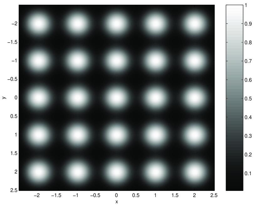
Figure 5:

(a)
(b)
(c)

Figure 6:

(a)
(b)
(c)

Figure 7:

(a)
(b)
(c)

Figure 8: