Abstract: Iterating between a router and a traffic micro-simulation is an increasibly accepted method for doing traffic assignment. This paper, after pointing out that the analytical theory of simulation-based assignment to-date is insufficient for some practical cases, presents results of simulation studies from a real world study. Specifically, we look into the issues of uniqueness, variability, and robustness and validation. Regarding uniqueness, despite some cautionary notes from a theoretical point of view, we find no indication of “meta-stable” states for the iterations. Variability however is considerable. By variability we mean the variation of the simulation of a given plan set by just changing the random seed. We show then results from three different micro-simulations under the same iteration scenario in order to test for the robustness of the results under different implementations. We find the results encouraging, also when comparing to reality and with a traditional assignment result.

Keywords: dynamic traffic assignment (DTA); traffic micro-simulation; TRANSIMS; large-scale simulations; urban planning

1 Introduction

Transportation-related decisions of people often depend on what everybody else is doing. For example, decisions about mode choice, route choice, activity scheduling, etc., can depend on congestion, caused by the aggregated behavior of others. From a conceptual viewpoint, this consistency problem causes a deadlock, since nobody can start planning because she does not know what everybody else is doing.

In fact, this problem is well-known not only in transportation, but in socio-economic systems in general. The traditional answer is to assume that everybody has complete information and is fully “rational”, i.e. that, for some given utility-function, each individual agent picks the solution that is best for herself. This means that each individual agent’s decision-making process now is globally known, and so each individual agent can (in principle) compute everybody else’s decision-making process conditioned on her own, and so she can arrive at a solution. As a side effect, since everybody arrives at the same solution for everybody, one can replace the individual decision-making process by a global computation.

Since this is a fictional process, one is traditionally not interested in the computation process itself, but just in the end result, which is a Nash equilibrium: Nobody can be better off by unilaterally changing strategies. Since only the end result is of interest, any algorithm finding that end result (assuming it is unique) is equally valid. In transportation, a typical example is the user equilibrium solution of the static assignment problem (e.g. Sheffi (1985)): No driver (or traffic stream) can be better off by switching routes. Thus, we assume that being at the equilibrium point is behaviorally justified, and everything we do in order to get there is just a mathematical or computational trick.

It is instructive to look at biological ecosystems for a minute. Here also, the behavior of everybody depends on everybody else. For example, an animal should not go to an area where predators catch it. Yet, since we assume that animals are less capable than humans to perform organized planning and reasoning, nobody ever assumed that animals would pre-compute an optimal solution based on some utility function. Instead, one formulates the problem as one of co-evolution, where everybody’s (mostly instinctive) behavior evolves in reaction to what is going on in the environment, constrained by the rules of genetical chemistry.

It is indeed this “eco-system” ($=$ agent-based) approach that more and more groups are also taking in the simulation of socio-economic problems. The advantage is that one does not have to make assumptions about properties of the system that are necessary in order to make the mathematics work. For example, one can just define rules on how agents decide on switching routes, both over night and on-line, and let the simulation run.

The disadvantage is that currently much less is known about the dynamical properties of such systems. The general question is how valid such approaches are for real-world problems. This includes the validity of the dynamics, the uniqueness of the solution, and the robustness of the solution towards changes in implementation. Non-uniqueness of solutions would be annoying although it may well be possible that this is a property of the real-world system. Robustness, i.e. that similar simulation methods yield similar results, is something we need to hope for because it will be hard to use such simulations in practice without it.

The work behind this paper is agent-based, since it simulates all individual entities of the traffic system, such as travelers, vehicles, signals, etc., as separate objects, all following their own rules and rules of interaction. For example, there is a plan for each individual traveler instead of origin-destination streams. The simulations use, however, also concepts from the traditional equilibrium approach, notably the idea that no traveler should be able to (significantly) improve by switching routes. It is in general not necessary to do this with a micro-simulation approach; we felt however that it would be better to start out this way before moving on to more uncertain terrain, such as truly behaviorally based decision rules.

This paper will, after a section about the problem formulation, first review static assignment (Sec. 3) and some theoretical results about simulation-based assignment (Sec. 4). In this, we will argue why we consider computational work a necessary complement to analytical progress. We will then proceed (Sec. 5) with a description of the real world scenario within which our computational studies were undertaken; we will also give a short description of the software modules that we used. The following sections (6–8) then describe results, in particular about uniqueness, variability, robustness and validation, and about alternative comparison measures. The paper is concluded by a summary.

2 Problem formulation: Dynamic traffic assignment

The problem treated in this paper is commonly referred to as dynamic traffic assignment, or DTA. In general, one is given information about the traffic network, plus a time-dependent origin-destination (OD) matrix which represents demand. The problem is to assign routes to each OD stream such the the result is “realistic”, which is often assumed to be the same as “in equilibrium”.

The main difference between most other simulation-based work (e.g. DYNAMIT (1999); Mahmassani et al. (1995)) and ours is that we are interested in an extremely disaggregated version of the problem: The transportation network comes with information such as number of lanes, speed limits, turn pockets, and signal phasing plans. And the demand is given in terms of individual trip plans, with a starting time, a starting location on the network, and a destination. Thus, writing this as a time-dependent OD-matrix is not really useful: First, since each link of the network is a potential origin or destination, one can easily obtain a matrix with 200 000 $\times$ 200 000 entries (TRANSIMS Portland case-study, in preparation). Second, our starting times come with second-by-second resolution. Translating this into second-by-second OD matrixes would result in matrices which are mostly empty, while aggregating it into longer time intervals means giving up information.

3 Static equilibrium assignment

This section contains a very short review of static equilibrium assignment, which is the traditional approach to our problem. The purpose of the section is not to discuss newest developments in the field (for a relatively recent review see, e.g., Patriksson (1994)), but to lay the ground work to point out certain similarities between traditional equilibrium assignment and current implementations of simulation-based assignment.

3.1 Deterministic User Equilibrium (UE) assignment

The traditional solution the problem of assigning traffic demand to routes in an urban planning scenario is static deterministic equilibrium assignment. For our case, this would be equivalent to a steady-state rate of travelers for each OD pair – anything in our plan-set that does not correspond to a steady state rate cannot be represented by static assignment.

Equilibrium assignment problems are usually posed in a way such that they have a unique solution (in terms of the link flows), and algorithms are known that come arbitrarily close to that solution. One important assumption is that the travel time on a link is a monotonically increasing function of the link flow – it is this assumption which is violated in practice since for all flow levels below capacity there are two corresponding travel time values. One iterative algorithm that comes arbitrarily close to the solution is the Frank-Wolfe algorithm. A possible interpretation of the Frank-Wolfe algorithm is as follows:

1. Use the current set of the link travel times and compute fastest paths for each OD stream (also called all-or-nothing assignment). If this is the first iteration, use free speed travel times.

2. Find a certain optimal convex combination between the set of path assignments that have been computed so far and this new set of assignments. In other words, for a certain fraction of the travelers, replace their paths by new ones.

3. Declare this combination the current set of paths. Calculate link travel times for it and start over.

This is repeated until some stopping criterion is met. This Frank-Wolfe algorithm is not the most efficient, but it is interesting because it resembles the iterated micro-simulation technique that we want to describe later in this text. For more information, see textbooks on the subject, e.g. Sheffi (1985).

3.2 Stochastic User Equilibrium (SUE) assignment

For stochastic assignment, one assumes that the route choice behavior of individual travelers has a random component – for example, because the information is noisy, or because there is a part of the cost function that cannot be explained by travel time, or because people’s perception is imprecise (Ben-Akiva and Lerman, 1985).

The standard approach to such problems is Discrete Choice Modeling (Ben-Akiva and Lerman, 1985). The outcome of this theory is that, for a given OD pair $rs$, each alternative route $k$ is chosen with probability $P_{k}$. Faster routes are still preferred over slower routes, but a certain fraction of the OD stream chooses the slower routes. Note that at this point the solution of the problem has been made deterministic, that is, all noise is moved into the distribution of the routes.

The solution to this is again unique under the usually assumed problem formulation – especially again that link travel time is a monotonically increasing function of link flow. An algorithm similar to the Frank-Wolfe algorithm can be shown to be applicable. A possible implementation of this (for a Probit choice model) is:

• Given (in Step 1 of the deterministic assignment algorithm in Sec. 3.1) the current set of link travel times, compute a Monte Carlo version of an all-or-nothing assignment. Monte Carlo here means that, for each OD pair, we randomly disturb the link travel times according to the Probit distribution and only then calculate the fastest path.

• In Step 2 of the deterministic assignment algorithm in Sec. 3.1, instead of calculating the optimal combination between the two sets of assignments, just use $1-1/n$ of the old set and $1/n$ of the new set where $n$ is the number of the iteration (method of successive averages).

In other words: One uses the best current estimate of link travel times, but then uses a noisy version of this to calculate a new assignment; and the fraction of the old assignment to be replaced is set to $1/n$.

4 Simulation-based assignment

As stated above, we want to solve a problem which is highly disaggregated and where the demand is given on a second-by-second basis. In addition, we assume that we are solving a real-world problem, which means besides other things that in principle we can get arbitrarily realistic network information.

There is by now some agreement that such problems can be approached with detailed micro-simulations. That is, once we have plans –which include starting times and exact routes– for each traveler, we can just feed this into a micro-simulation and extract any performance measure such as time-dependent link travel times from the simulation. Based on these performance measures, we can change the plans of some or all of the travelers, re-run the micro-simulation, etc., until some kind of relaxation criterion is met.

Let us introduce some minimal notation. Each user $u$ chooses a route $r_{u}$. Given $N$ users, then the set of these routes is $\vec{R}=(r_{1},\ldots,r_{N})$. Recall that each route includes a starting time. The resulting link costs are $\vec{C}=(c_{1},\ldots,c_{L})$, where $L$ is the number of links. $\vec{C}$ depends on the time-of-day, i.e. $\vec{C}=\vec{C}(t)$. In iterated micro-simulations, there are two transitions:

1. the simulation (also called network loading model):

   $$S:\vec{R}\to\vec{C}\ ,$$

   and

2. the route assignment:

   $$A:\vec{C}\to\vec{R}\ .$$

Both mappings can be deterministic or stochastic.

Our problem can then be formulated as an iterated map (Cascetta, 1989; Cascetta and Cantarella, 1991). One can see it as an iterated map both in the routes or in the costs: $\vec{R}^{n}\to\vec{R}^{n+1}$ or $\vec{C}^{n}\to\vec{C}^{n+1}$ (Bottom, in preparation; Bottom et al., 1998). A fix point would be reached if, e.g., $\vec{R}^{n+1}\equiv A\circ S(\vec{R}^{n})=\vec{R}^{n}$. If at least one of the mappings $S$ or $A$ is stochastic, then one cannot expect to reach a fix-point; however, one can hope to reach a steady state density: $p(\vec{R}^{n+1})=p(\vec{R}^{n})$.

As a side remark, note that one can also formulate this as a continuous dynamical system by making $n$ continuous; the mapping $A\circ S$ would then be replaced by a differential equation. Such systems (e.g. Friesz et al. (1994)), although related, are somewhat more removed from the topic of this paper since iterated versions of dynamical systems can display vastly different dynamics from their continuous counterparts (e.g. Schuster (1995)).

The stochastic user equilibrium case could be modeled by assuming that we have as many “users” as we have routes for each OD relation $rs$, together with a traffic stream strength $q_{u}^{rs}$. The mapping $S$ is then simply the typical link cost function. That is, link flows are the sum of all OD streams that pass over the current link, and link cost is a function of link flow. The mapping $A:\vec{C}\to\vec{R}$ would come from the particular “re-planning” algorithm that was selected for the SUE problem, for example from a Monte Carlo assignment plus the method of successive averages. One can for example search for a fix-point in $\vec{C}$, i.e. $\vec{C}^{n+1}=C^{n}$.

For the more general problem of time-dependent assignment, one would like to show similar things as one has shown for the equilibrium assignments: for example uniqueness, and an algorithm that is guaranteed to converge. Indeed, it can be shown (Cascetta, 1989; Cascetta and Cantarella, 1991) that under certain circumstances the mapping $A\circ S:\vec{R}\to\vec{R}$ is ergodic, which means that any combination of feasible routes will eventually be used by the iterations. “Feasible routes” is a set of routes that brings the traveler from her starting location to her destination; in general, it is a finite set since one assumes that routes are loopless. This means that every combination of routes has a time-invariant probability $p(\vec{R})$ to be used, and since the system is ergodic, in order to obtain mean values one can replace the phase-space average $\langle X\rangle=\sum_{\vec{R}}p(\vec{R})\cdot X(\vec{R})$ by an iteration average $\overline{X}^{T}=1/T\sum_{n=i}^{i+T}X(\vec{R}^{n})$, where $n$ and $i$ are iteration indices.

The in our view most critical condition for this to be true is that

• either each feasible route has a probability larger than zero to be selected in the following time step (Cascetta, 1989) $(*)$

• or each set of feasible routes can be reached from any other set of feasible routes via a sequence of iterations (Cascetta and Cantarella, 1991). $(**)$

For practical applications, however, the situation is more complicated. We want to point out three examples of possible problems with the analytical results. We and others have never observed these problems in the practice of simulation-based DTA; however, they indicate that systematic simulations or an improvement of the theory are necessary. The examples come from Palmer (1989), which is an introduction to the phenomenon of broken ergodicity, which is one of the possible problems one might face. The first two examples can be found in most textbooks on Statistical Physics.

• First, ergodicity is actually not enough to ensure that the phase space density (i.e. the space of all possible route sets) becomes uniform and stationary. For example, it would be ergodic to sort all feasible route sets into a sequence and only allow transitions along the sequence. A more stringent property called “mixing” is needed to cause any initial phase space distribution (which in our case is just a point: one set of routes) to spread uniformly. $(*)$ will ensure mixing, $(**)$ will not.

• Second, ergodicity only says something for the infinite time limit; it might take much longer than the age of the universe for an actual ergodic system to do a good job of covering the phase space.

• Third, the system may show broken ergodicity. That is, the system may be quasi-ergodic in a part of the phase space, with very little yet non-zero probability of escaping from that part. Our iterative assignment may be “stuck” with a particular type of solution for a very large number of iterations; if we do not run enough iterations, we will never see that there is another type of solution. Sometimes, one calls these states “meta-stable”, but that word makes the situation sound less problematic than it potentially can be.

In consequence, in this paper we want to report simulation experiments with highly disaggregated DTAs in large realistic networks. First, we look into uniqueness of the simulation results. Second, we are interested in how “robust” our results are. We want define “robustness” more in terms of common sense than in terms of a mathematical formalism. For this, we do not only want a single iterative process to “converge”, but we want the result to be independent of any particular implementation. In consequence, we run many computational experiments, sometimes with variations of the same code, sometimes with totally different code, in order to see if any of our results are robust against these changes. Part of the robustness analysis is a validation, since we compare some results to field measurements, where available. Last, we will argue that there may be better ways to compare simulations than the typical link-by-link analysis, and show an example. Before we do all this, however, we need to describe our study set-up.

5 Context

5.1 Dallas/Fort Worth Case study

The context of the work done for this paper is the so-called Dallas–Fort Worth case study of the TRANSIMS project (Beckman et al, 1997). Most of the details relevant for the present paper can also be found in Nagel and Barrett (1997). The purpose of the case study was to show that a micro-simulation based approach to transportation planning such as promoted by TRANSIMS will allow analysis that is difficult or impossible with traditional assignment, such as measures of effectiveness (MOE) by sub-populations (stakeholder analysis), in a straightforward way. In the following we want to mention the most important details of the case study set-up; as said, more information can be found in Beckman et al (1997) and Nagel and Barrett (1997).

The underlying road network for the study (public transit was not considered) was a so-called focused network, which had 14751 mostly bi-directional links and 9864 nodes. Out of those, 6124 links and 2292 nodes represented all roads in a 5 miles times 5 miles study area, whereas the network got considerably “thinner” with further distance from the study area. A picture of the focused network can be found in Nagel and Barrett (1997).

The TRANSIMS design specifies to use demographic data as input and generate, via synthetic households and synthetic activities, the transportation demand. The Dallas/Fort Worth case study was based on interim technology: part of the demand generation was not available then. For that reason, we use a standard time-dependent OD matrix as a starting point, which is immediately broken down into individual trips. All trips are routed through the empty network, and only trips that go through our smaller study area are retained. This base set contains approx. 300 000 trips. Note that this defines a base set of trips for all subsequent studies presented in this paper: All trips thrown out before can no longer influence the result of the studies, although they may in reality. Again, more information can be found in Beckman et al (1997) and Nagel and Barrett (1997).

5.2 The micro-simulations

The above procedure does not only generate a base set of trips, but also an initial set of routes (called initial planset). These routes are then run through a micro-simulation, where each individual route plan is executed subject to the constraints posed by the traffic system (e.g. signals) and by other vehicles. Note that this implies that the micro-simulation is capable of executing pre-computed routes (only very few micro-simulation had this capability when this work was done although their number is growing), and it also implies that, in the simulations, drivers do not have the capability of changing their routing on-line. Three micro-simulations are used, all three related to the TRANSIMS project, but with different levels of realism and different intended usages. We will call them TR (for TRANSIMS micro-simulation), PA (for PAMINA), and QM (for Queue Model). TR is the most realistic one, QM the least realistic ones of the three. The first two micro-simulations are based on the so-called cellular automata technique for traffic flow (Nagel et al. (1998) and references therein). The third one uses a simple queueing model (Gawron, 1998; Simon and Nagel, 1999).

The TRANSIMS micro-simulation (TR). TR is the “mainstream” TRANSIMS micro-simulation. As said above, it is the most realistic of the three, including elements such as number of lanes, speed limits, signal plans, weaving and turn pockets, lange changing both for vehicle speed optimization and for plan following, etc. The studies described in this paper were run on five coupled Sun Sparc 5 workstations which ran the micro-simulation on the given problem as fast as real time; newer versions of this micro-simulation also run on a SUN Enterprise 4000. Details of TR can be found in Nagel et al. (1997) and in TRANSIMS (since 1992).

The PAMINA micro-simulation (PA). The second micro-simulation, PA, uses simplified signal plans, and it does neither include pocket lanes nor lane changing for plan following. Most other specifications are the same as for TR, although differences can be caused by the different implementation. PA is much better optimized for high computing speed: it ran more than 20 times faster than TR for this study, which is a combined effect of using faster hardware (it is much easier to port to different hardware, thus being able to take advantage of new and faster hardware much sooner), less realism, and an implementation oriented towards computational speed. This micro-simulation is documented in Rickert (1998), Gawron et al. (1997), and Rickert and Nagel (1997).

The Queue Model micro-simulation (QM). The QM micro-simulation uses simple FIFO queues for the link exits. These queues have a service rate equivalent to the link capacity. The main difference to other queueing models, e.g. Simão and Powell (1992), is that in our model each link has a limited “storage capacity”, representing the number of vehicles that can sit on the link at jam density. This results in the capability to model queue spill-back across intersections, a very important feature of congested traffic.

When a car enters a link at time $t_{enter}$, an expected link travel time, $T_{free}$, is calculated using the length and the free flow speed of the link. The vehicle is then put into the queue, together with a time $t_{dep1}=t_{enter}+T_{free}$ which marks the earliest possible departure at the other end of the link. In each time step, the queue is checked if the first vehicle can leave according to $t_{dep1}$, according to the capacity constraints, and according to the storage constraints of the destination link. The queue is served until one of these conditions is not fulfilled. The spirit of the model is also similar to earlier versions of INTEGRATION (INTEGRATION, 1994). For further details on QM, see Simon and Nagel (1999).

The reason for having a model like this is that we want a micro-simulation model that fits into the overall TRANSIMS framework (i.e. runs on individual, pre-computed plans) but has much less computational and data requirements than the other simulation models. Indeed, QM runs on the same data as traditional assignment models, and on a single CPU it is computationally a factor 20 faster than PA. A parallel version is planned.

5.3 Router

Our micro-simulations run on precomputed route plans, i.e. on a link-by-link list which connects the starting point with the destination. For our studies, we use a time-dependent Dijkstra fastest path algorithm. Link travel times are, during the simulation, averaged into 15-minute bins. These 15-minute bins give the link costs for the Dijkstra algorithm (Jacob et al., in press). The Dallas study makes no attempt to include alternative modes of transportation, such as walking, bicycle, or public transit.

We want to mention here that, in earlier versions, we randomly disturbed link travel times by $\pm 30\%$ in order to spread out the traffic. This would be very similar to what some implementations of Stochastic User Equilibrium (SUE) assignment (Sec. 3.2) do. We found, however, that this led to many undesirable paths, for example cars leaving the freeway and re-entering at the same entry/exit. In general, it is rather difficult to find “reasonable” path alternatives different from the optimal path (Park and Rilett, 1997). We would therefore expect that also the standard SUE approach, when applied to large networks, would display such unrealistic artifacts.

5.4 Feedback iterations and re-planning

The initial planset is obviously wrong during heavy traffic because drivers have not adjusted to the occurence of congestion. In reality, drivers avoid heavily congested segments if they can. We model that behavior by using iterative re-planning: The micro-simulation is run on a pre-computed planset and travel times along links are collected. Then, for a certain fraction, $f$, of the drivers, new routes are computed based on these link travel times. Technically, each route from the old planset is read in, with probability $1-f$ it is written unchanged into a new file, and with probability $f$ a new route is computed given the starting time, starting location, and destination location from the old route plus the time-dependent link travel times provided by the last iteration of the micro-simulation. In consequence, $f$ is the re-planning fraction. After this, the micro-simulation is run again on the new planset, more drivers are re-routed, etc., until the system is “relaxed”, i.e. no further changes are observed from one iteration to the next except for fluctuations (all three micro-simulations are stochastic).

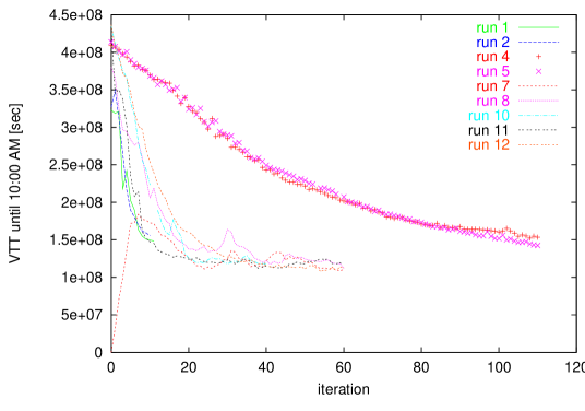
Figure 1: Sum of all trip times (system-wide Vehicle Time Travelled) for different iteration series. For details see Rickert (1998). All iteration series relax towards the same VTT, which indicates (but does not prove) that all series releax towards the same traffic scenario.

6 Uniqueness

By uniqueness we want to refer to a property that the same combination of router and microsimulation, with the same input data, generates via the relaxation procedure the same traffic scenario. This still allows for differences in the random seeds, in the way one selects travelers for re-planning, etc. We have run (Rickert, 1998) many relaxation experiments with different re-planning mechanisms, including an incremental network loading over 20 iterations, a very slow iteration series with 1% replanning fraction, and different ways of picking the travellers that are replanned. We have not found any indication that any of those relaxations ran into a traffic scenario that was different from the other ones.

This means that in spite of the cautionary note in Sec. 4 regarding broken ergodicity etc., practical implementations of DTA seem to be well-behaved in this regard. This is consistent with observations from other groups (e.g. Wagner (personal communication)) and also from experiments involving human subjects (Mahmassani et al., 1986).

As a side remark, it may be worth mentioning that the best-performing relaxation method was similar to the method of successive averages (MSA). What we call “age-dependent re-planning” (Rickert, 1998) started in practice with a 30% replanning fraction, which slowly decreased to 5% in the 20th iteration. MSA by comparison uses $1/n$ as the replanning fraction, where $n$ is the iteration number. Clearly, MSA also interpolates from high replanning fractions at the beginning to 5% at the 20th iteration. However, age-dependent re-planning also moves through the population in a systematic way, which is more than what MSA does. More systematic comparisons between these methods should be tried.

7 Variability

Note that any given iteration $n$ corresponds to a certain set of route plans $\vec{R}^{n}$. For that reason, one can just re-run the simulation of these route plans, i.e. just the mapping $S$. If one uses a different random seed, this leads to a different traffic scenario. These differences (not to confuse with possible differences caused by broken ergodicity) could be quite large in our experiments. An example can be found in Nagel (1998), which shows link density plots for two simulations of exactly the same route plan sets but with different random seeds. The microsimulation that was used was the TRANSIMS micro-simulation, i.e. TR. In one simulation (the “exceptional” traffic pattern), vehicles were unable to get off a freeway fast enough, thus blocking the freeway, thus causing queue spillback through a significant part of the network. In the other simulation (the “generic” traffic pattern, which we also found with many more other random seeds), this heavy queue spill-back did not occur.

We have repeated these variability investigations with a Portland (Oregon) scenario and a different micro-simulation – indeed the QM queue micro-simulation from this paper. During those investigations, we found that such strong variations depend, as one might expect, heavily on the congestion level: They do not occur for low demand but become more and more frequent when demand rises (B. Raney et al, unpublished).

An interesting comparison can be made between the sources and handling of noise in Stochastic User Equilibrium (SUE) assignment and our method. SUE assignment has at every iteration a “best estimate” of link travel times. A possible implementation of SUE assignment is to take a deliberately randomized realization of those link travel times, to re-route a fraction of the population on those, and then to take this new combined route set and to compute the new resulting link travel times.

Instead of deliberately randomizing our best estimate of link travel times, we use a stochastic microsimulation which on its own generates variability of link travel times. The advantage of our method may be that the noise is actually directly generated by the traffic system dynamics – one should therefore assume that for example correlations between links will be considerably more realistic as with the parametrized noise approach of the SUE assignment. In contrast to SUE, however, we use the same random realization for all re-planned routes. If one route is, via a fluctuation, fast in this realization, it will be fast for all OD pairs and thus attract a considerable amount of new traffic. This causes local oscillations, which are avoided in the SUE approach. However, remember that we would expect unrealistic routes with some SUE implementations, see Sec. 5.3.

8 Robustness and Validation

As stated above, we mean by robustness the reproducibility of results under different implementations. Discussion of driving rules (mostly car following, lane changing, and gap acceptance) is a necessary part of this, but it is not sufficient and somewhat misleading since it does not put enough emphasis on the actual traffic outcome of the simulation. We propose at least two “macroscopic” tests:

1. “Building block tests”: Test simple situations, such as traffic in a closed loop, unprotected turn flows, etc. See Nagel et al. (1997) for a discussion of this.

2. “Real situation tests”: Compare the results of different micro-simulations under the same scenario. This is the topic of this section.

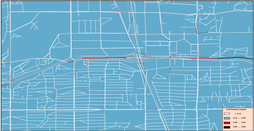
Figure 2: TRANSIMS 14b 8:00 AM

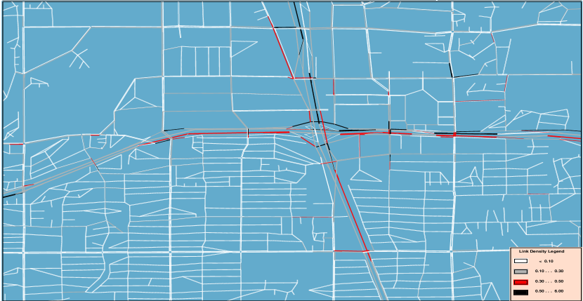
Figure 3: PAMINA 8:00 AM

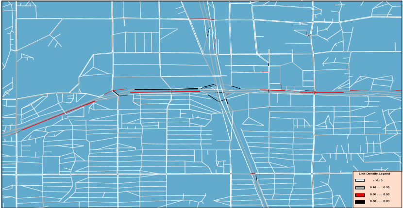
Figure 4: QM 8:00 AM

8.1 Visual comparison of link densities

In our case, we did the same re-planning scenario, as described in Sec. 5.4, with three different micro-simulations, as described in Sec. 5.2. Visual comparisons of typical relaxed traffic patterns at 8:00am are shown in Figs. 2 to 4. In our view, there is a remarkable degree of “structural” similarity between the plots. This becomes particularly clear if one compares where the simulations predict bottlenecks, which are in general at the downstream end of congested pieces.

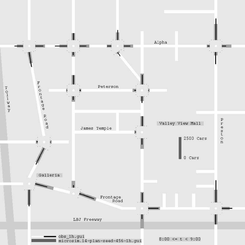
Figure 5: Approach volumes from the TRANSIMS micro-simulation series compared to field data. The wide gray bars are the simulation results; the narrow black bars are the field data. The freeway intersection in the bottom left corner of this figure is in the center of the study area as can be seen in Figs. 2 to 3.

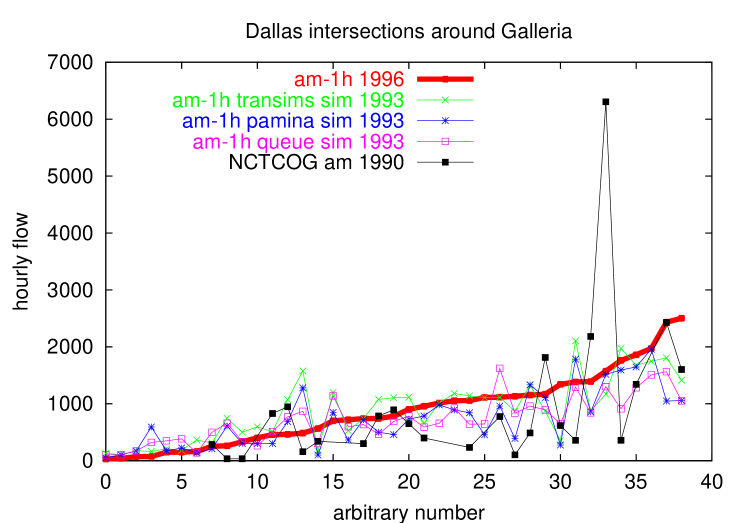
Figure 6: Approach volumes for the links shown in Fig. 5. The links are sorted according to increasing flow in the field data, which is denoted by the wide line. The different points in different shades of gray denote simulation results as denoted in the legend; the black line shows the NCTCOG assignment result. Lines are included to guide the eye.

$$\halign to=433.62pt{$\hfil#$\ \ && \hfil# \cr\hrule\vskip 3.0pt plus 1.0pt minus 1.0pt\hrule\vskip 3.0pt plus 1.0pt minus 1.0pt\cr\hbox{Class} &$N$&TR\hfil&PA\hfil&QM\hfil&$N_{COG}$&NCTCOG\cr\vskip 3.0pt plus 1.0pt minus 1.0pt\hrule\vskip 3.0pt plus 1.0pt minus 1.0pt\cr\leq 250 : &7&0.960294&1.217647&1.391176\cr 251 - 500 : &7&1.004520&0.639925&0.577778&6\hfil&0.774523\cr 501 - 750 : &5&0.409052&0.354857&0.347362&3\hfil&0.346680\cr 751 - 1000 : &3&0.317941&0.252839&0.218395&3\hfil&0.348600\cr 1001 - 1500 : &11&0.245609&0.325389&0.307282&8\hfil&0.620177\cr\geq 1501 : &6&0.226150&0.271165&0.370695&5\hfil&0.745831\cr\vskip 3.0pt plus 1.0pt minus 1.0pt\hrule\vskip 3.0pt plus 1.0pt minus 1.0pt\cr}$$

Table 1: Comparison between field data and simulation results. Shown is the average relative error, i.e. $\langle|N_{field}-N_{sim}|/N_{field}\rangle$, where the averages are separate for different flow levels. The first column shows the boundaries of the classes, in vehicles per hour. The second column shows the number of entries per class. The third, fourth, and fifth column show results for the different micro-simulations, TR, PA, and QM, respectively. The sixth column shows again the number of entries per class, this time for the NCTCOG assignment; column number seven finally shows the results for the NCTCOG assignment. For the TR, PA, QM, and NCTCOG columns, lower values are better.

8.2 Quantitative comparison of approach counts; validation

A quantitative analysis of the above results would be useful, but is beyond the scope of this paper. Instead, we want to turn to link exit volume results for a smaller number of links, which have the advantage that comparison data from reality is available. Note that the field data is from 1996, whereas the demand for our simulations is from 1990. Thus, one would expect that there is more traffic in the field data. Fig. 5 shows a graphical comparison for the TR micro-simulation result. In general, it seems that we are underestimating traffic, as we had expected. However, we have a tendency to overpredict traffic on low priority links. This is probably because our router is based on travel time only, and does not include relevant other measures such as convenience.

Fig. 6 compares exit counts for all links that we had field data for. The links are sorted according to increasing flow in the field data. Indeed, both PA and QM are somewhat underestiming the flows, although TR in the average does not do so. This was also the result of a wider comparison using other data (Beckman et al, 1997).

We also include results from an assignment done by the local transportation planning authority, the North-Central Texas Council of Governments, NCTCOG. Unfortunately, the NCTCOG assignment data and the field data are not really comparable since the NCTCOG assignment was made for a different network than our simulations and the field measurements. In particular, the north extension of the Dallas North Tollway had not been built, which is the freeway extending from the interchange in the center of the study area to the north. A result of this is that in the NCTCOG assignment the freeway connects to a frontage road. This is what leads to the high assigned volume for link 32. One should recognize that this is a physically impossible solution since a signalized 3-lane road cannot carry 6000 vehicles per hour. A simulation-based method would have generated a totally different result in the same situation.

Table 1 gives a quantitative summary of the same data. What is shown is the mean relative percentage deviation from the field value, i.e.

$$dev={1\over N}\sum_{a}{|x_{a}^{field}-x_{a}^{sim}|\over x_{a}^{field}}\ ,$$

where the sum goes over all links $a$ in a class, $N$ is the number of links in that class, and $x_{a}^{field}$ and $x_{a}^{sim}$ are the volume counts from the field data and from the simulation, respectively. Thus, a low value of $dev$ means a small relative difference to reality. According to the table, classes go from 0 to 250 vehicles per hour, from 251 to 500 vehicles per hour, etc. The table first gives the class, then the number of count sites available for this class, then the values of $dev$ for the different models. This is followed by data for the NCTCOG assignment, where another column of the number of count sites is given since the NCTCOG results were only available for a smaller number of links (that assignment was run on a reduced network).

In spite of the difference regarding the freeway extension between the NCTCOG result and our simulation results we believe that the comparison between our results and the NCTCOG assignment allows the following two conclusions:

1. Our simulation-based results already at this early stage of the technology development yield forecast quality which is comparable to traditional assignment.

2. The three micro-simulations generate results that are remarkably similar in structure. This indicates that demand generation research is currently at least as important as micro-simulation research.

Figure 7: “Geometrical” mean speeds into the study-area, i.e. geometrical distance between origin and destination divided by trip time. The $x$-axis shows the starting time for the trips.

8.3 Comparisons using accessibility

Often, transportation engineers use aggregated measures of system performance (Measures of Effectiveness, MOEs) such as vehicle miles traveled (VMT), the sum of all traveled distances in the system. A similar measure are “geometrical” mean speeds, which are a measure of accessibility. In our situation, we collected for all vehicles with their origin outside the study area and their destination inside the study area their geometrical distance, $d$, between origin and destination, and their travel time, $T$. $d/T$ is then the “geometrical” speed for a traveler, a measure of how fast she makes progress towards her destination. We see (Fig. 7) that during the rush hour, the results of TR, PA and for QM are practically identical. In uncongested situations, PA predicts faster travel than QM which predicts faster travel than TR. This effect can be traced back to the fact that (due to an implementation error) the maximum average speed in TR was 75 km/h (47 MPH), in PA it was the correct design value of 103 km/h (64 MPH), in QM it was set to the average free flow speed which is slightly lower than PA’s average speed limit. Therefore, in uncongested situations, the predicted travel times clearly have to be systematically different.

This indicates that aggregated measures can be considerably more robust than more disaggregated ones. In order to economize resources, one should therefore pay close attention to the question at hand – quite possibly, available models can give a robust answer for that question even when they fail to reproduce reality on a link-by-link basis. This is, however, naturally also a question for further research: Under what circumstances can we trust such aggregate measures even when the simulation results are not close to reality on a more disaggretaged level?

9 Summary and discussion

In this paper, we reported computational experiments with large scale dynamic traffic assignments (DTA) in the context of a Dallas scenario. An important difference of our approach to many other investigations is that our approach is completely disaggregated, i.e. we treat individual travelers from the beginning to the end. We also used a relatively large network, with 6124 links, where the restriction to the network size came from data availability, not from the capabilities of our methods. We pointed out that although some theory is available for DTAs, this theory needs to be used with care for typical simulation-based DTA scenarios with a small number of iterations. For that reason, computational experiments remain a necessity.

We started by looking for indications of non-uniqueness of the solution, i.e. that different set-ups of the iterations could lead to different relaxed traffic scenarios. We did not find any indication that this had happened in our situation. We did, however, find instances of very strong variability of the simulation itself, i.e. the mapping $S$ from route plans to traffic, which is stochastic. The reason for this is that the links are not independent; a queue which is caused by a “normal” fluctuation may spill back through large parts of the system.

We then moved to the issue of “robustness”, by which we mean that different implementations should yield comparable results in the same scenarios. In consequence, we implemented three different micro-simulations and ran them with the same input data and the same re-planning algorithms. Comparisons between those results, and also to field data and to a traditional assignment result, indicate that (1) simulation-based assignment is already at the current stage of research of similar quality as traditional (equilibrium) assignment, and (2) contributions to deviations from field data come probably as much from the demand generation as from the micro-simulations.

We concluded by arguing that a link-by-link comparison of performances is not necessarily what one wants in order to evaluate a result. As an example, we showed a curve for accessibility of a certain area in the micro-simulation as a function of time-of-day, and we pointed out that for the critical part of the morning, which is the rush hour, the curves for the three simulation methods are practically identic.

References

- Beckman et al (1997) Beckman et al, R., 1997. TRANSIMS–Release 1.0 – The Dallas-Fort Worth case study. Los Alamos Unclassified Report (LA-UR) 97-4502, see transims.tsasa.lanl.gov.
- Ben-Akiva and Lerman (1985) Ben-Akiva, M., Lerman, S. R., 1985. Discrete choice analysis. The MIT Press, Cambridge, MA.
- Bottom et al. (1998) Bottom, J., Ben-Akiva, M., Bierlaire, M., Chabini, I., 1998. Generation of consistent anticipatory route guidance. In: Proceedings of TRISTAN III, vol. 2. San Juan, Puerto Rico.
- Bottom (in preparation) Bottom, J. A., in preparation. Ph.D. thesis, Massachusetts Institute of Technology, Cambridge, MA.
- Cascetta (1989) Cascetta, E., 1989. A stochastic process approach to the analysis of temporal dynamics in transportation networks. Transportation Research B, 23B(1), 1–17.
- Cascetta and Cantarella (1991) Cascetta, E., Cantarella, C., 1991. A day-to-day and within day dynamic stochastic assignment model. Transportation Research A, 25A(5), 277–291.
- DYNAMIT (1999) DYNAMIT, 1999. DYNAMIT. Massachusetts Institute of Technology, Cambridge, Massachusetts. See its.mit.edu.
- Friesz et al. (1994) Friesz, T. L., Bernstein, D., Mehta, N. J., Tobin, R. L., Ganjalizadeh, S., 1994. Day-to-day dynamic network disequilibria and idealized traveler information systems. Operations Research, 42(6), 1120–1136.
- Gawron (1998) Gawron, C., 1998. An iterative algorithm to determine the dynamic user equilibrium in a traffic simulation model. International Journal of Modern Physics C, 9(3), 393–407.
- Gawron et al. (1997) Gawron, C., Rickert, M., Wagner, P., 1997. Real-time simulation of the German autobahn network. In: Proc. of the 4th Workshop on Parallel Systems and Algorithms (PASA ‘96), edited by F. Hoßfeld, E. Maehle, E. Mayer. World Scientific Publishing Co.
- INTEGRATION (1994) INTEGRATION, 1994. INTEGRATION: A model for simulating IVHS in integrated traffic networks, User’s guide for model version 1.5e. Transportation Systems Research Group, Queens’ University and M. Van Aerde and Associates, Ltd.
-
Jacob et al. (in press)
Jacob, R. R., Marathe, M. V., Nagel, K., in press.
A computational study of routing algorithms for realistic
transportation networks.
ACM Journal of Experimental Algorithms.
See www.inf.ethz.ch/
~nagel/papers. - Mahmassani et al. (1986) Mahmassani, H., Chang, G.-L., Herman, R., 1986. Individual decisions and collective effects in a simulated traffic system. Transportation Science, 20(4), 258.
- Mahmassani et al. (1995) Mahmassani, H., Hu, T., Jayakrishnan, R., 1995. Dynamic traffic assignment and simulation for advanced network informatics (DYNASMART). In: Urban traffic networks: Dynamic flow modeling and control, edited by N. Gartner, G. Improta. Springer, Berlin/New York.
- Nagel (1998) Nagel, K., 1998. Experiences with iterated traffic microsimulations in Dallas. In: Traffic and granular flow’97, edited by D. Wolf, M. Schreckenberg, pages 199–214. Springer, Heidelberg.
- Nagel and Barrett (1997) Nagel, K., Barrett, C., 1997. Using microsimulation feedback for trip adaptation for realistic traffic in Dallas. International Journal of Modern Physics C, 8(3), 505–526.
-
Nagel et al. (1997)
Nagel, K., Stretz, P., Pieck, M., Leckey, S., Donnelly, R., Barrett, C. L.,
1997.
TRANSIMS traffic flow characteristics.
Los Alamos Unclassified Report (LA-UR) 97-3530, see
www.inf.ethz.ch/
~nagel/papers. Earlier version: Transportation Research Board Annual Meeting paper 981332. - Nagel et al. (1998) Nagel, K., Wolf, D., Wagner, P., Simon, P. M., 1998. Two-lane traffic rules for cellular automata: A systematic approach. Physical Review E, 58(2), 1425–1437.
- Palmer (1989) Palmer, R., 1989. Broken ergodicity. In: Lectures in the Sciences of Complexity, edited by D. L. Stein, vol. I of Santa Fe Institute Studies in the Sciences of Complexity, pages 275–300. Addison-Wesley.
- Park and Rilett (1997) Park, D., Rilett, L. R., 1997. Identifying multiple and reasonable paths in transportation networks: A heuristic approach. Transportation Research Records, 1607, 31–37.
- Patriksson (1994) Patriksson, M., 1994. The Traffic Assignment Problem: Models and Methods. Topics in Transportation. VSP, Zeist, The Netherlands.
-
Rickert (1998)
Rickert, M., 1998.
Traffic simulation on distributed memory computers.
Ph.D. thesis, University of Cologne, Germany.
See www.zpr.uni-koeln.de/
~mr/dissertation. - Rickert and Nagel (1997) Rickert, M., Nagel, K., 1997. Experiences with a simplified microsimulation for the Dallas/Fort Worth area. International Journal of Modern Physics C, 8(3), 483–504.
- Schuster (1995) Schuster, H. G., 1995. Deterministic Chaos: An Introduction. Wiley-VCH Verlag GmbH.
- Sheffi (1985) Sheffi, Y., 1985. Urban transportation networks: Equilibrium analysis with mathematical programming methods. Prentice-Hall, Englewood Cliffs, NJ, USA.
- Simão and Powell (1992) Simão, H., Powell, W., 1992. Numerical methods for simulating transient, stochastic queueing networks. Transportation Science, 26, 296.
- Simon and Nagel (1999) Simon, P. M., Nagel, K., 1999. Simple queueing model applied to the city of Portland. International Journal of Modern Physics C, 10(5), 941–960. Earlier version Transportation Research Board Annual Meeting paper 99 12 49.
- TRANSIMS (since 1992) TRANSIMS, since 1992. TRANSIMS, TRansportation ANalysis and SIMulation System. See transims.tsasa.lanl.gov.
- Wagner (personal communication) Wagner, P., personal communication.