Stability of Oscillating Hexagons in Rotating Convection

Abstract

Breaking the chiral symmetry, rotation induces a secondary Hopf bifurcation in weakly nonlinear hexagon patterns which gives rise to oscillating hexagons. We study the stability of the oscillating hexagons using three coupled Ginzburg-Landau equations. Close to the bifurcation point we derive reduced equations for the amplitude of the oscillation, coupled to the phase of the underlying hexagons. Within these equation we identify two types of long-wave instabilities and study the ensuing dynamics using numerical simulations of the three coupled Ginzburg-Landau equations.

1 Introduction

Convection has played a key role in the elucidation of the spatio-temporal dynamics arising in non-equilibrium pattern forming systems. The interplay of well-controlled experiments with analytical and numerical theoretical work has contributed to a better understanding of various mechanisms that can lead to complex behavior. From a theoretical point of view the effect of rotation on roll convection has been particularly interesting because it can lead to spatio-temporal chaos immediately above threshold where the small amplitude of the pattern allows a simplified treatment. Early work of Küppers and Lortz [1, 2] showed that for sufficiently large rotation rate the roll pattern becomes unstable to another set of rolls rotated with respect to the initial one. Due to isotropy the new set of rolls is also unstable and persistent dynamics are expected. Later Busse and Heikes [3] confirmed experimentally the existence of this instability and the persistent dynamics arising from it. They proposed an idealized model of three coupled amplitude equations in which the instability leads to a heteroclinic cycle connecting three sets of rolls rotated by 120^o with respect to each other. Recently the Küppers-Lortz instability and the ensuing dynamics have been subject to intensive research, both experimentally [4, 5, 6, 7, 8] and theoretically [9, 10, 11, 12, 13, 14, 15]. It is found that in sufficiently large systems the switching between rolls of different orientation looses coherence and the pattern breaks up into patches in which the rolls change orientation at different times. The shape and size of the patches changes persistently due to the motion of the fronts separating them.

In this paper we are interested in the effect of rotation on hexagonal rather than roll (stripe) patterns as they arise in systems with broken up-down symmetry (e.g. non-Boussinesq or surface-tension driven convection with rotation). The dynamics of strictly periodic hexagon patterns with broken chiral symmetry have been investigated in detail by Swift [16] and Soward [17]. They found that the heteroclinic orbit of the Busse-Heikes model is replaced by a periodic orbit arising from a secondary Hopf bifurcation off the hexagons. Their results have been confirmed in numerical simulations of a Swift-Hohenberg-type model [18] in which an alternation among the three modes that compose the hexagonal pattern is observed. In the following we will call this state ‘oscillating hexagons’. The oscillations can be homogeneous in space or can take on the form of traveling waves. Starting from coupled Ginzburg-Landau equations, we have previously derived evolution equations for the oscillating hexagons that are valid close to the Hopf bifurcation. Within this framework the oscillating hexagons were found to support a state of spatio-temporal chaos that is characterized by defects, in which the oscillation amplitude vanishes [19]. At the band center the oscillating hexagons and their chaotic state are described by the single complex Ginzburg-Landau equation (CGLE). In general, however, the oscillation amplitude is coupled to the phases of the underlying pattern as it is to be expected for a secondary bifurcation. Here we study how this coupling affects the stability of the oscillations. In particular, it will modify the stability properties of the waves emitted by the spirals in the defect chaotic state. We find that the additional coupling leads to new long-wave instabilities if the rotation is strong enough or if the wavenumber of the hexagons is far away from the band-center.

The paper is organized as follows. In the second section we introduce the appropriate coupled Ginzburg-Landau equations that describe the hexagon patterns and derive the amplitude-phase equations close to the secondary Hopf bifurcation. The stability analysis of these equations is addressed in section III. In section IV we study numerically the behavior resulting from these instabilities. Conclusions are given in section V. Details of the calculations are given in two appendices.

2 Amplitude-Phase equations for Oscillating Hexagons

We consider small-amplitude hexagon patterns in systems with broken chiral symmetry. In order to analyze the possibility of modulational instabilities we include spatial derivatives. Due to the strong coupling between modes of different orientation, we take the gradients in both directions to be of the same order and retain only linear gradient terms (a study of the influence of nonlinear gradient terms in the stability of oscillating hexagons is addressed in appendix B). After rescaling the amplitude, time, and space we arrive at the equations,

$$\partial_{t}A_{1} = \mu A_{1}+({\bf{n}}_{1}\cdot\nabla)^{2}A_{1}+\overline{A}_{2}\overline{A}_{3}-A_{1}|A_{1}|^{2}$$

$$-(\nu+\gamma)A_{1}|A_{2}|^{2}-(\nu-\gamma)A_{1}|A_{3}|^{2},$$

where the equations for the other two amplitudes are obtained by cyclic permutation of the indices and $\mu$ is a parameter related to the distance from threshold. The overbar represents complex conjugation. These equations can be obtained from the corresponding physical equations (e.g. Navier-Stokes) using a perturbative technique. The broken chiral symmetry manifests itself by the cross-coupling coefficients not being equal. Hence $\gamma$ is a measure of rotation.

For completeness it should be noted that rotation leads in convection not only to a chiral symmetry breaking but also to a (weak) breaking of the translation symmetry due to the centrifugal force. In the following we will consider it to be negligible. We focus on not too small Prandtl numbers, in which case the primary bifurcation is always steady [24, 13].

Equation (2) admits hexagon solutions $A_{j}=Re^{iq\hat{\bf n}_{j}\cdot{\bf{x}}+i\phi_{j}}$ with a slightly off-critical wavenumber ($\tilde{\bf q}_{j}=\tilde{\bf q}^{c}_{j}+{\bf q}_{j}$, $|{\bf q}_{j}|\ll|\tilde{\bf q}_{c}|\equiv\tilde{q}_{c}$), with

$$R=\frac{1\pm\sqrt{1+4(\mu-q^{2})(1+2\nu)}}{2(1+2\nu)},\qquad\Phi\equiv\phi_{1}+\phi_{2}+\phi_{3}=0.$$ (2)

The stability of this solution to perturbations with the same wave vectors has been studied by several authors [16, 17]. Typical results are sketched in the bifurcation diagrams shown in Fig. 1. The hexagons appear through a saddle-node bifurcation at $\mu=\mu_{sn}$,

$$\mu_{sn}=-\frac{1}{4(1+2\nu)}+q^{2},$$ (3)

and become unstable via a Hopf bifurcation at $\mu=\mu_{H}$, with a frequency $\omega_{H}$,

$$\mu_{H}=\frac{(2+\nu)}{(\nu-1)^{2}}+q^{2},\;\;\omega_{H}=2\sqrt{3}\gamma/(\nu-1)^{2}.$$ (4)

The Hopf bifurcation is supercritical and for $\mu>\mu_{H}$ stable oscillations in the three amplitudes of the hexagonal pattern arise with a phase shift of $2\pi/3$ between them [16, 17, 18], resulting in what we call oscillating hexagons. As $\mu$ is increased further, eventually a point $\mu=\mu_{het}$ is reached at which the branch of oscillating hexagons ends on the branch corresponding to a mixed-mode solution in a global bifurcation involving a heteroclinic connection (see Fig. 1a). Above this point the only stable solution is the roll solution whose stability region is bounded below by

$$\mu_{R}=\frac{1}{(\nu+\gamma-1)(\nu-\gamma-1)}+q^{2}.$$ (5)

From Eqs. (4), (5) it is easy to see that, when $\gamma^{2}>(\nu-1)(\nu+1)/(\nu+2)$, the transition to oscillating hexagons occurs at a value of $\mu$ for which the rolls are still unstable. There is then a parameter regime in which the oscillating hexagons are the only stable solution. Furthermore, when $|\gamma|>\nu-1\equiv\gamma_{KL}$ rolls are never stable and the limit cycle persists for arbitrarily large values of $\mu$ (see Fig. 1b). In the absence of the quadratic terms in Eq. (2) this condition corresponds to the Küppers-Lortz instability of rolls. When the quadratic term in Eq. (2) is small (i.e. small non-Boussinesq effects) it can be considered as a perturbation of the usual three mode model for rotating roll convection. Far above the Hopf bifurcation ($\mu\gg\mu_{H}$) the periodic orbit is expected to become asymmetrical and the resulting state similar to that encountered in the usual rotating Rayleigh-Bénard convection.

         

Figure 1: Sketch of a bifurcation diagram for a fixed value of the wavenumber $q$. a) For $\gamma<\gamma_{{KL}}$ limit cycle of oscillating hexagons ends via heteroclinic cycle and rolls become stable. b) For $\gamma>\gamma_{KL}$ oscillating hexagons persist and rolls do not become stable.

The stability of steady hexagons with respect to side-band perturbations in the presence of rotation has been studied previously [25]. Due to the rotation steady and oscillatory, long-wave and short-wave instabilities have been found. It turns out that in the presence of rotation the steady hexagons can be stable up to the Hopf bifurcation over quite a range of wavenumbers. Thus, the oscillating hexagons may be stable near the Hopf bifurcation.

The focus of the present paper are side-band instabilities of the oscillating hexagons. To address this question analytically we focus on the vicinity of the Hopf bifurcation where the oscillation amplitude is small and a weakly nonlinear analysis is possible. Since we are dealing with a secondary bifurcation the two phases of the underlying hexagons have to be taken into account as well. In fact, from a linear stability analysis of Eq. (2) it is easy to see that there are four marginal modes at $\mu=\mu_{H}$. Two correspond to the Hopf bifurcation and can be described by a complex amplitude ${\cal H}$. The other two correspond to a two-dimensional phase vector $\vec{\phi}$, related to translations in the x- and y-directions [26, 27]. It can be written as a combination of the phases of the three modes: $\vec{\phi}=(\phi_{x},\phi_{y})\equiv(-\phi_{2}-\phi_{3},(\phi_{2}-\phi_{3})/\sqrt{3})$, satisfying the locking condition $\phi_{1}+\phi_{2}+\phi_{3}=\Phi$. The global phase $\Phi$ is a fast variable that relaxes rapidly to its stationary values $\Phi=0,\pi$ (up or down hexagons). To study the nonlinear behavior of the oscillating hexagons, the amplitudes $A_{i}$ are expanded as:

$$A_{n}=(R_{H}+e^{2\pi ni/3}\sqrt{\epsilon}{\cal H}e^{i\omega_{H}t}+c.c.+{\cal O}(\epsilon))e^{i{\bf q}_{i}\cdot{\bf x}+\sqrt{\epsilon}\phi_{i}},$$ (6)

where $\epsilon$ is a small parameter related to the distance from the bifurcation line. The amplitude of the steady hexagons at the bifurcation point, $R_{H}=1/(\nu-1)$, is independent of $\mu$ and $q$. Eliminating the fast variables, at order $\epsilon^{3/2}$ (see appendix A) we arrive at an equation for the amplitude of the oscillation ${\cal H}$, coupled to the phase vector of the underlying hexagonal pattern,

$$\partial_{T}{\cal H} = \varepsilon\delta_{1}{\cal H}+\xi\nabla^{2}{\cal H}-\delta_{2}{\cal H}\nabla\cdot\vec{\phi}-\rho{\cal H}|{\cal H}|^{2},$$ (7)

$$\partial_{T}\vec{\phi} = D_{\bot}\nabla^{2}\vec{\phi}+D_{\|}\nabla(\nabla\cdot\vec{\phi})+D_{\times_{1}}({\bf e}_{z}\times\nabla^{2}\vec{\phi})$$

$$+D_{\times_{2}}({\bf e}_{z}\times\nabla)(\nabla\cdot\vec{\phi})+\alpha\nabla|{\cal H}|^{2}+\beta_{1}({\bf e}_{z}\times\nabla)|{\cal H}|^{2}$$

$$-i\beta_{2}({\cal H}\nabla\overline{{\cal H}}-\overline{{\cal H}}\nabla{\cal H})+i\eta[{\cal H}({\bf e}_{z}\times\nabla)\overline{{\cal H}}-\overline{{\cal H}}({\bf e}_{z}\times\nabla){\cal H}],$$

with $\varepsilon=\mu-\mu_{H}$ and

$$v=3R_{H}(1+2R_{H}),$$ (9)

$$\delta_{1}=\frac{2R_{H}}{v}-\frac{2i\omega_{H}}{v},\;\;\delta_{2}=q\delta_{1},$$ (10)

$$\xi=\frac{1}{2}-\frac{3q^{2}R_{H}}{9R_{H}^{2}+\omega_{H}^{2}}-\frac{iq^{2}}{\omega_{H}}\frac{9R_{H}^{2}+2\omega_{H}^{2}}{9R_{H}^{2}+\omega_{H}^{2}},$$ (11)

$$\rho=\frac{8(3R_{H}+1)}{v}-\frac{4i\omega_{H}(1+4R_{H})}{R_{H}v}-\frac{32i}{3\omega_{H}},$$ (12)

$$D_{\bot}=\frac{1}{4},\;\;D_{\|}=\frac{1}{2}-\frac{2q^{2}}{v},\;\;D_{\times_{1}}=\frac{q^{2}}{\omega_{H}},\;\;D_{\times_{2}}=0,$$ (13)

$$\alpha=-\frac{2\omega_{H}^{2}q}{9R_{H}^{2}+\omega_{H}^{2}}-\frac{2q(1+6R_{H})}{R_{H}v},$$ (14)

$$\beta_{1}=\frac{6\omega_{H}q}{R_{H}(9R_{H}^{2}+\omega_{H}^{2})},\;\;\beta_{2}=\beta_{1},\;\;\eta=\frac{18q}{9R_{H}^{2}+\omega_{H}^{2}}.$$ (15)

It is worth pointing out that the phase-amplitude equations (7,2) can be deduced by means of symmetry arguments alone and are, therefore, generic to this order in $\epsilon$. In fact, they could be derived directly from the fluid equations without the use of the Ginzburg-Landau equations (2). Thus, keeping higher order terms in (2) would change the values of the coefficients, but not their form.

When deriving (7,2) using symmetry arguments, one interesting aspect has to be taken into account. In most secondary bifurcations, the oscillating amplitude is either even or odd under reflection symmetry (see, for instance, [20]). In our case, however, the field ${\cal H}$ transforms under reflection ${\bf x}\rightarrow-{\bf x}$ as ${\cal H}\rightarrow\overline{\cal H}$. The temporal phase of this complex amplitude is therefore a pseudo-scalar, changing sign under reflection. This is because this phase is related to the oscillating frequency which, in turn, depends linearly on the chiral symmetry breaking coefficient ($\omega_{H}=2\sqrt{3}R_{H}^{2}\gamma$). This implies that, in Eq. (2), the term $({\cal H}\nabla\overline{{\cal H}}-\overline{{\cal H}}\nabla{\cal H})$ breaks the chiral symmetry, but not the term $[{\cal H}({\bf e}_{z}\times\nabla)\overline{{\cal H}}-\overline{{\cal H}}({\bf e}_{z}\times\nabla){\cal H}]$, as one could have naively expected. Looking at the values for the coefficients we see that, in fact, $\beta_{2}$ changes sign while $\eta$ is invariant under $\omega_{H}\rightarrow-\omega_{H}$.

It is interesting to note that at the band-center ($q=0$) the system (7,2) decouples. In this case the usual CGLE for the amplitude of the oscillation is recovered, which after rescaling the amplitude, time, and space can be written as [28]:

$$\partial_{t}H=H+(1+ib_{1})\nabla^{2}H-(b_{3}-i\;{\rm sign}(\omega_{H}))H|H|^{2},$$ (16)

with

$$b_{1}=\frac{\xi_{i}}{\xi_{r}}=\frac{2(R_{H}^{2}+2\omega_{H}^{2})q^{2}}{(2q^{2}R_{H}-R_{H}^{2}-\omega_{H}^{2})\omega_{H}},$$ (17)

$$b_{3}=-\frac{\rho_{r}}{|\rho_{i}|}=\frac{2|\omega_{H}|R_{H}(3R_{H}+1)}{\omega_{H}^{2}(1+4R_{H})+8R_{H}^{2}(1+2R_{H})},$$ (18)

where the sub-indices r and i indicate real and imaginary part, respectively. Furthermore, at the band-center $b_{1}=0$.

The CGLE has been studied extensively. It possesses an extraordinary variety of solutions, including a phase chaotic state, defect chaos, a frozen vortex state and stable plane waves [28, 29, 30, 31, 32, 33, 34, 35]. For the case considered here the values of the parameters $b_{1}$ and $b_{3}$ are always such that the system is in a regime in which stable plane waves coexist with defect chaos. In the present context it has to be emphasized that the complex amplitude of the CGLE represents the amplitude of oscillation of the hexagon pattern. Thus, a solution of Eq. (7) with spatially uniform amplitude ${\cal H}=He^{i\Omega t}$,

$$H=\sqrt{\frac{\varepsilon\delta_{1r}}{\rho_{r}}}=\sqrt{\frac{\varepsilon R_{H}}{4(1+3R_{H})}},\makebox[28.45274pt]{}\Omega=\delta_{1i}\varepsilon-\rho_{i}H^{2},$$ (19)

corresponds to a state in which all three amplitudes oscillate in time phase-shifted with respect to each other but the phase of each amplitude is constant in space, as illustrated in Fig. 2. In a traveling wave solution (TW),

$${\cal H}=He^{i\Omega t+i{\bf k}\cdot{\bf x}},$$ (20)

with

$$H=\sqrt{\frac{\varepsilon\delta_{1r}-\xi_{r}k^{2}}{\rho_{r}}},\;\;\;\Omega=\varepsilon(\delta_{1i}-\frac{\rho_{i}}{\rho_{r}}\delta_{1r})-(\xi_{i}-\frac{\rho_{i}}{\rho_{r}}\xi_{r})k^{2},\;\;k=|{\bf k}|,$$ (21)

the phase of each amplitude is space dependent and in different parts of the system roll-like hexagons with different orientation are dominant at any given time. This is shown in Fig. 3. Note that such a state has two different wavenumbers: that of the underlying regular hexagon pattern and that of the wave modulating the oscillation amplitude. At the band-center, i.e. for hexagons that have the critical wavenumber, the modulation of the oscillation amplitude does not affect the phase of the underlying hexagons.

           

           

Figure 2: Oscillating hexagons ($\mu=4.6$, $\nu=2$, $\gamma=0.5$, $L=200$, ${\bf k}=0$, $q=0$, $\tilde{q}_{c}=0.44$). There is one period of oscillation between the first and last snapshots. The contour lines are taken at $\psi=\sum^{3}_{j=1}A_{j}e^{i\tilde{\bf q}^{c}_{j}\cdot{\bf x}}=-1,0,1$.

           

           

Figure 3: Traveling hexagons ($\mu=4.6$, $\nu=2$, $\gamma=0.5$, $L=200$, $k_{x}=0.0628$, $k_{y}=0$, $q=0.125$, $\tilde{q}_{c}=0.31$). There is one period of oscillation between the fist and last snapshots. The modulation is traveling with phase velocity: $v_{ph}=(\omega_{H}+\Omega)/k\simeq 27.27$. The underlying hexagons are traveling with a speed: $v=2H^{2}\sqrt{\beta_{2}^{2}+\eta^{2}}/\tilde{q}\simeq 0.00035$, too small to be observed in the figures.

Away from the band-center ($q\neq 0$) the complex amplitude ${\cal H}$ and the phase vector $\vec{\phi}$ become coupled. For the traveling-wave state of the oscillation amplitude (20) this implies that even the underlying hexagon pattern drifts with a velocity that depends on the wave vector of the modulation. Specifically, the phase is given by $\vec{\phi}=\vec{\omega}t$, with

$$\vec{\omega}=-2H^{2}[\beta_{2}{\bf k}-\eta(\hat{\bf e}_{z}\times{\bf k})],$$ (22)

which implies a drift of the hexagons with a speed $v=2H^{2}\sqrt{\beta_{2}^{2}+\eta^{2}}/\tilde{q}$, at an angle $\theta=\arctan(-\eta/\beta_{2})$ with respect to the wave vector of the traveling wave. Substituting the values of the coefficients (9-15) one obtains for the angle $\theta=\arctan(3R_{H}/\omega_{H})$. Thus, for $\omega_{H}\;\rightarrow 0$ the angle becomes $\theta=\pm\pi/2$, i.e. the drift is perpendicular to the wave vector of the modulation. When $\omega_{H}\rightarrow\infty$, on the other hand, they drift in the parallel direction ($\theta\;\rightarrow\;0,\pi$). The speed $v$ is given by

$$v=4\left(\frac{H}{R_{H}}\right)^{2}\frac{qk}{\tilde{q}\sqrt{1+\left(\frac{\omega_{H}}{3R_{H}}\right)^{2}}}.$$ (23)

The traveling waves exist above the curve $\varepsilon\delta_{1r}-\xi_{r}k^{2}=0$, up to the global bifurcation at $\mu=\mu_{het}$. However they can be unstable to side-band perturbations. In the following we study their stability properties. In particular, we will focus on the effect of the coupling of the oscillation amplitude ${\cal H}$ to the phase of the underlying hexagons.

3 Linear stability analysis

To consider the linear stability of the oscillating hexagons, we perturb the traveling-wave state (20) as

$${\cal H}=(H+h)e^{i(\Omega t+{\bf k}\cdot{\bf x}+\varphi)},\;\;\;\vec{\phi}=\vec{\omega}t+\vec{\phi}_{1}.$$ (24)

For simplicity we write $\vec{\phi}_{1}$ in the following as $\vec{\phi}$. Substituting (24) in Eqs. (7,2) we obtain the linear equations for the perturbations:

$$\partial_{T}h = -2\xi_{r}H{\bf k}\cdot\nabla\varphi-2\xi_{i}{\bf k}\cdot\nabla h+\xi_{r}\nabla^{2}h-\xi_{i}H\nabla^{2}\varphi-\delta_{2r}H\nabla\cdot\vec{\phi}$$

$$-2\rho_{r}H^{2}h,$$

$$\partial_{T}\varphi = -2\xi_{i}{\bf k}\cdot\nabla\varphi+\frac{2\xi_{r}}{H}{\bf k}\cdot\nabla h+\xi_{r}\nabla^{2}\varphi+\frac{\xi_{i}}{H}\nabla^{2}h-\delta_{2i}\nabla\cdot\vec{\phi}-2\rho_{i}Hh,$$ (26)

$$\partial_{T}\vec{\phi} = D_{\bot}\nabla^{2}\vec{\phi}+D_{\|}\nabla(\nabla\cdot\vec{\phi})+D_{\times_{1}}\nabla^{2}({\bf e}_{z}\times\vec{\phi})+D_{\times_{2}}({\bf e}_{z}\times\nabla)(\nabla\cdot\vec{\phi})$$

$$+2\alpha H\nabla h+2\beta_{1}H({\bf e}_{z}\times\nabla)h-2\beta_{2}H^{2}\nabla\varphi+2\eta H^{2}({\bf e}_{z}\times\nabla)\varphi$$

$$-4\beta_{2}Hh{\bf k}+4\eta Hh(\hat{\bf e}_{z}\times{\bf k}).$$

This leads to a $4\times 4$ linear eigenvalue problem, which must be solved numerically. In the long-wave limit the perturbation in the amplitude $h$ becomes slaved to the gradients of the phases $\varphi$ and $\vec{\phi}$. The resulting $3\times 3$ system is, however, still rather involved. A substantial simplification occurs in the case ${\bf k}=0$, i.e. for homogeneously oscillating hexagons. In order to gain physical insight we will consider this case first.

3.1 Homogeneous Oscillations

For homogeneously oscillating hexagons $\vec{\omega}=0$ and the perturbation equations (3,26,3) reduce to

$$\partial_{T}h = \xi_{r}\nabla^{2}h-\xi H\nabla^{2}\varphi-\delta_{2r}H\nabla\cdot\vec{\phi}-2\rho_{r}H^{2}h,$$ (28)

$$\partial_{T}\varphi = \xi_{r}\nabla^{2}\varphi+\frac{\xi_{i}}{H}\nabla^{2}h-\delta_{2i}\nabla\cdot\vec{\phi}-2\rho_{i}Hh,$$ (29)

$$\partial_{T}\vec{\phi} = D_{\bot}\nabla^{2}\vec{\phi}+D_{\|}\nabla(\nabla\cdot\vec{\phi})+D_{\times_{1}}\nabla^{2}({\bf e}_{z}\times\vec{\phi})+D_{\times_{2}}({\bf e}_{z}\times\nabla)(\nabla\cdot\vec{\phi})$$ (30)

$$+2\alpha H\nabla h+2\beta_{1}H({\bf e}_{z}\times\nabla)h-2\beta_{2}H^{2}\nabla\varphi+2\eta H^{2}({\bf e}_{z}\times\nabla)\varphi.$$

In the limit of long-wave perturbations the amplitude $h$ can be eliminated adiabatically

$$h\simeq\frac{1}{2\rho_{r}H^{2}}[-\xi_{i}H\nabla^{2}\varphi-\delta_{2r}H\nabla\cdot\vec{\phi}].$$ (31)

In this manner we arrive at a system for the three phases, two corresponding to the spatial translations in the plane, the other to a temporal shift,

$$\partial_{T}\vec{\phi} = D_{\bot}\nabla^{2}\vec{\phi}+\left(D_{\|}-\frac{\alpha\delta_{2r}}{\rho_{r}}\right)\nabla(\nabla\cdot\vec{\phi})+D_{\times_{1}}\nabla^{2}({\bf e}_{z}\times\vec{\phi})$$ (32)

$$+\left(D_{\times_{2}}-\frac{\beta_{1}\delta_{r}}{\rho_{r}}\right)({\bf e}_{z}\times\nabla)(\nabla\cdot\vec{\phi})-\frac{\alpha\xi_{i}}{\rho_{r}}\nabla^{2}(\nabla\varphi)$$

$$-\frac{\beta_{1}\xi_{i}}{\rho_{r}}\nabla^{2}({\bf e}_{z}\times\nabla)\varphi-2\beta_{2}H^{2}\nabla\varphi+2\eta H^{2}({\bf e}_{z}\times\nabla)\varphi,$$

$$\partial_{T}\varphi = \left(\xi_{r}+\frac{\rho_{i}}{\rho_{r}}\xi_{i}\right)\nabla^{2}\varphi+\left(\delta_{2r}\frac{\rho_{i}}{\rho_{r}}-\delta_{2i}\right)\nabla\cdot\vec{\phi}.$$ (33)

At the band-center, $q=0$, Eqs. (7,2) decouple since $\beta_{1}=\beta_{2}=\delta_{2}=\alpha=\eta=0$ (cf. (9-15)). It is easy to show that in that case the eigenvalues are

$$\sigma_{1,2}=-\frac{1}{2}\left[2D_{\bot}+D_{\|}\pm\sqrt{D_{\|}^{2}-4D_{\times_{1}}(D_{\times_{1}}+D_{\times_{2}})}\right]Q^{2},$$ (34)

$$\sigma_{3}=-\left(\xi_{r}+\frac{\rho_{i}}{\rho_{r}}\xi_{i}\right)Q^{2}.$$ (35)

We obtain therefore the usual expression for the phase instabilities of the underlying hexagons [25] and the Benjamin-Feir instability of the oscillations [36]. The actual values of these eigenvalues, when $q=0$, are $\sigma_{1}=-Q^{2}/4$, $\sigma_{2}=-3Q^{2}/4$ and $\sigma_{3}=-Q^{2}/2$. The system is therefore always stable at the band-center.

Away from the band-center ($q\neq 0$) the system is no longer decoupled. At leading order in the long-wave expansion (32), (33) we have then

$$\partial_{T}{\vec{\phi}} = -2\beta_{2}H^{2}\nabla\varphi+2\eta H^{2}(\hat{e}_{z}\times\nabla)\varphi,$$ (36)

$$\partial_{T}\varphi = \left(\delta_{2r}\frac{\rho_{i}}{\rho_{r}}-\delta_{2i}\right)\nabla\cdot\vec{\phi}.$$ (37)

These two equations can be combined into a single second-order equation for $\vec{\phi}$,

$$\partial^{2}_{T}\vec{\phi}=-2\left(\delta_{2r}\frac{\rho_{i}}{\rho_{r}}-\delta_{2i}\right)H^{2}(\beta_{2}\nabla-\eta(\hat{e}_{z}\times\nabla))(\nabla\cdot\vec{\phi}).$$ (38)

Writing in normal modes, $\phi_{x}=\phi^{0}_{x}e^{i{\bf Q}\cdot{\bf x}+\sigma t}$, $\phi_{y}=\phi^{0}_{y}e^{i{\bf Q}\cdot{\bf x}+\sigma t}$, $\varphi=\varphi^{0}e^{i{\bf Q}\cdot{\bf x}+\sigma t}$, $Q\equiv|{\bf Q}|$, we arrive at the dispersion relation

$$\sigma_{1} = 0,$$ (39)

$$\sigma_{2,3} = \pm\sqrt{2\left(\delta_{2r}\rho_{i}/\rho_{r}-\delta_{2i}\right)\beta_{2}}\,HQ,$$ (40)

indicating the possibility of two different instabilities.

The eigenvalue $\sigma_{1}$ corresponds to the divergence-free part of $\vec{\phi}$ and does not involve $\varphi$ (cf. Eq. (37)). It is marginal at this order. The eigenmodes associated with $\sigma_{2,3}$ involve both phases $\vec{\phi}$ and $\varphi$. For $\gamma^{2}>2/(3R_{H}^{2})$, $\sigma_{2}$ is always positive (except at the band-center, where $\beta_{2}=0$). Hence there exists a critical value for the rotation $|\gamma_{c}|\equiv\sqrt{2/3}/R_{H}$ above which the system is unstable for $Q\rightarrow 0$. When $|\gamma|<|\gamma_{c}|$ the eigenvalues $\sigma_{2,3}$ are purely imaginary and the stability is determined at next order.

At quadratic order in the perturbation wavenumber $Q$ one obtains

$$\sigma_{1} = \left(-D_{\bot}+\frac{\eta}{\beta_{2}}D_{\times_{1}}\right)Q^{2},$$ (41)

$$\sigma_{2,3} = \pm\sqrt{2H^{2}\beta_{2}\left(\delta_{2r}\frac{\rho_{i}}{\rho_{r}}-\delta_{2i}\right)}\,Q$$

$$-\frac{1}{2}\left(D_{\bot}+D_{\|}-\alpha\frac{\delta_{2r}}{\rho_{r}}+\beta_{2}\frac{\delta_{2r}\rho_{i}}{\rho_{r}^{2}}+\frac{\eta}{\beta_{2}}D_{\times_{1}}+\xi_{r}+\frac{\rho_{i}}{\rho_{r}}\xi_{i}\right)\,Q^{2}.$$

Substituting the values of the coefficients from (9-15) in $\sigma_{1}$ we see that it becomes positive provided $q^{2}>\gamma^{2}R_{H}^{3}$. In Fig. 4a the long-wave stability limits of the oscillating hexagons are shown for $\nu=2$ and $\gamma=0.5$. These results agree with those obtained solving the full $4\times 4$ dispersion relation. Hence, for any given value of the rotation rate there is a value of the wavenumber above which the system becomes unstable. The range of stable wavenumbers decreases as the rotation rate is decreased. In fact, it vanishes as $\gamma\rightarrow 0$. In this limit also the range in $\varepsilon$ over which the oscillating hexagons exist vanishes. Also shown in Fig. 4a are the instabilities of steady hexagons, below the Hopf bifurcation. The solid line represents the long-wave results, while the circles are the results obtained solving the $6\times 6$ dispersion relation associated with Eq. (2) [25]. The dash-dotted line represents the line above which the rolls become stable (cf. Eq. (5)).

As $\gamma$ is increased the range of wavenumbers that are stable with respect to the diffusive mode ($\sigma_{1}<0$) increases. However, for $\gamma>\gamma_{c}$, $\sigma_{2}$ becomes positive for $Q\rightarrow 0$. In finite systems the term quadratic in $Q$ may not be negligible. In fact, inserting the values from (9-15) into Eq. (3.1) shows that the $Q^{2}$-term in $\sigma_{2,3}$ is always stabilizing when $q\ll 1$ ($\sigma_{2}=\sigma_{3}=-5Q^{2}/8$, when $q=0$), and for $q\sim{\cal O}(1)$ it is only destabilizing when $\gamma,\nu\gg 1$. For $q=1$ typical values of $\gamma,\nu$ for which this happens are $\nu\simeq 30,\gamma\simeq 70$. Therefore, in finite systems, in which $Q_{\rm min}=2\pi/L$ cannot be arbitrarily small, there is always a region close to the band-center that is stable, even when $|\gamma|>|\gamma_{c}|$. The stability limit $\sigma_{2}=0$ is given by an expression of the form $H^{2}\sim\mu-\mu_{H}=f(q)/(Lq^{2})$, where $f(q)$ appears due to the $q$-dependence of the second term in (3.1). This situation is shown in Fig. 4b, where the different symbols correspond to several values of the system size. For smaller systems the stable region increases. The shape of the stability limits suggest that $f(q)$ does not depend strongly on $q$. In Fig. 4b the instability corresponding to $\sigma_{1}>0$ has moved to higher values of $q$ ($q=\pm 0.9$).

Figure 4: Stability limits of oscillating hexagons ($\nu=2$, $\gamma_{c}=0.816$). Lines indicate saddle-node for hexagons (dotted), Hopf bifurcation (dashed) and stability limits for rolls against hexagons (dot-dashed). a) $\gamma=0.5<\gamma_{c}$. b) $\gamma=0.9>\gamma_{c}$. Symbols indicate different system sizes, L=250 (circles), 500 (squares) and 1000 (diamonds). The stable region close to the band-center shrinks as the system size is increased.

It should be noted that taking the limit $q\rightarrow 0$ in (41), (3.1) does not give the same results as in (34), (35). In fact, in the limit $q\rightarrow 0$, the three eigenvalues in (41), (3.1) become $\sigma_{1}=-Q^{2}/4$, $\sigma_{2}=\sigma_{3}=-5Q^{2}/8$, while Eqs. (34), (35) yield $\sigma_{2}=-3Q^{2}/4$ and $\sigma_{3}=-Q^{2}/2$. This difference is due to the fact that, in order to obtain (41) and (3.1) we assume $q$ to be ${\cal O}(1)$, and expand in terms of $Q$, while (34) and (35) are obtained by taking the limit $q\rightarrow 0$ first. If we consider both to be small and of the same order, $q\sim Q\ll 1$, then:

$$\sigma_{1} = -D_{\bot}Q^{2}$$ (43)

$$\sigma_{2,3} = -\frac{1}{2}(D_{\bot}+D_{\|}+\xi_{r})Q^{2}$$

$$\pm\left[2H^{2}\beta_{2}\left(\delta_{2r}\frac{\rho_{i}}{\rho_{r}}-\delta_{2i}\right)+\frac{1}{4}(D_{\bot}+D_{\|}-\xi_{r})^{2}Q^{2}\right]^{1/2}Q.$$

When $q=0$ we obtain $\sigma_{1}=-Q^{2}/4$, $\sigma_{2}=-3Q^{2}/4$ and $\sigma_{3}=-Q^{2}/2$, while considering $Q\ll q$ expressions (39), (40) are recovered at leading order.

3.2 Stability of Traveling Waves

For the traveling waves the expressions become quite complicated. We therefore present the analytical results from the long-wave analysis only up to linear order in the gradients. As in the case of homogeneous oscillations, in the long-wave limit $h$ becomes slaved (cf. (3)),

$$h\simeq\frac{1}{2\rho_{r}H^{2}}[-2\xi_{r}H({\bf k}\cdot\nabla)\varphi-\delta_{2r}H(\nabla\cdot\vec{\phi})].$$ (45)

At the band-center $\vec{\phi}$ and $\varphi$ decouple and we recover expression (34) for the eigenvalues $\sigma_{1,2}$ associated with $\vec{\phi}$. The eigenvalue $\sigma_{3}$ describes the long-wave behavior of the single CGLE. It is given by

$$\sigma_{3}=i{\bf v}_{g}\cdot{\bf Q}+2(1+\frac{\rho_{i}^{2}}{\rho_{r}^{2}})\frac{\xi_{r}^{2}({\bf k}\cdot{\bf Q})^{2}}{\varepsilon\delta_{1r}-\xi_{r}k^{2}}-(\xi_{r}+\frac{\rho_{i}}{\rho_{r}}\xi_{i})Q^{2},$$ (46)

and yields the usual Eckhaus stability limit for waves. Here we have introduced the group velocity

$${\bf v}_{g}\equiv\frac{\partial\Omega}{\partial{\bf k}}=-2(\xi_{i}-\frac{\rho_{i}}{\rho_{r}}\xi_{r}){\bf k}.$$ (47)

The expression $\varepsilon\equiv\mu-\mu_{H}=\xi_{r}k^{2}/\delta_{1r}$ gives the neutral surface for the appearance of traveling waves of wavenumber ${\bf k}$.

Away from the band-center Eqs. (3,26,3) reduce at leading order in the long-wave expansion to

$$\partial_{T}{\vec{\phi}} = \frac{4\xi_{r}}{\rho_{r}}[\beta_{2}{\bf k}-\eta(\hat{\bf e}_{z}\times{\bf k})]({\bf k}\cdot\nabla)\varphi+\frac{2\delta_{2r}}{\rho_{r}}[\beta_{2}{\bf k}-\eta(\hat{\bf e}_{z}\times{\bf k})](\nabla\cdot\vec{\phi})$$

$$-2H^{2}[\beta_{2}\nabla\varphi-\eta(\hat{e}_{z}\times\nabla)\varphi],$$

$$\partial_{T}\varphi = -2(\xi_{i}-\frac{\rho_{i}}{\rho_{r}}\xi_{r}){\bf k}\cdot\nabla\varphi+\left(\delta_{2r}\frac{\rho_{i}}{\rho_{r}}-\delta_{2i}\right)\nabla\cdot\vec{\phi}.$$ (49)

This yields the eigenvalues

$$\sigma_{1} = 0$$ (50)

$$\sigma_{2,3} = \frac{i}{2}\left({\bf v}_{g}+\frac{\delta_{2r}}{\rho_{r}}{\bf v}_{h}\right)\cdot{\bf Q}\pm\left\{-\frac{1}{4}\left[\left({\bf v}_{g}+\frac{\delta_{2r}}{\rho_{r}}{\bf v}_{h}\right)\cdot{\bf Q}\right]^{2}\right.$$

$$\left.+\frac{4}{\rho_{r}}(\delta_{2r}{\bf v}_{g}\cdot{\bf Q}-\xi_{r}\Gamma{\bf k}\cdot{\bf Q})({\bf v}_{g}\cdot{\bf Q})+2H^{2}\beta_{2}\Gamma Q^{2}\right\}^{1/2},$$

where we have defined $\Gamma\equiv\delta_{2r}\rho_{i}/\rho_{r}-\delta_{2i}$ and ${\bf v}_{h}\equiv-\vec{\omega}/(2H^{2})$ (cf. (22)).

Since the analytical expressions for the eigenvalues are quite complicated we solve Eqs. (3,26,3) directly without the additional long-wave approximation (45) for various values of the wavenumber ${\bf k}=(k,0)$ of the traveling waves. Fig. 5a shows the neutral surface of traveling waves and their stability limit as a function of the hexagon wavenumber $q$. Due to the reflection symmetries $q\rightarrow-q$ and $k\rightarrow-k$ only one quadrant is shown. For clarity the stability surface has been capped at $\mu=6$. For $k=0$ the stability limit does not depend on $\mu$ and the stability surface is vertical (cf. Fig. 4a). As $k$ is increased the stability surface becomes smoother. For $k\neq 0$, the waves are unstable at onset and become stable above the second surface. Fig. 5b shows cross-sections of the stability surface for $\gamma>\gamma_{c}$, for a system of size $L=250$. When $k=0$ we recover the results from Fig. 4b. For $k\neq 0$, but small (cf. $k=0.1$ in Fig. 5b) the traveling waves are unstable at onset but they become stable for larger values of $\mu$. When $|q|$ is large they can become unstable again as $\mu$ is increased. For larger values of $k$, the latter two stability lines merge and the stability region becomes bounded in $q$. At this point the stability limits in Figs. 5a and 5b look similar.

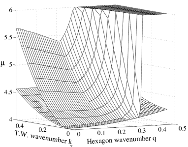
Figure 5: Stability limits of traveling waves ($\nu=2$, $\gamma_{c}=0.816$). a) $\gamma=0.3<\gamma_{c}$. Shown are the neutral surface and the stability limit. Traveling waves are stable above the second surface. b) $\gamma=0.9>\gamma_{c}$. Dashed-dotted line: stability limit of rolls against hexagons.

4 Numerical simulations

In order to study the nonlinear behavior arising from the instabilities, we have performed numerical simulations of Eqs. (2) and (7), (2). A Runge-Kutta method with an integrating factor that computes the linear derivative terms exactly has been used. Derivatives were computed in Fourier space, using a two-dimensional fast Fourier transform (FFT). The numerical simulations were done in a rectangular box of aspect ratio $2/\sqrt{3}$ with periodic boundary conditions. This aspect ratio was used to allow for regular hexagonal patterns.

We investigate the stability of oscillating hexagons simulating both the original amplitude equations (2) and the reduced amplitude-phase equations (7), (2). To that end, we start with homogeneously oscillating hexagons as given by Eq. (19) (or Eq. (6)) and add weak noise. For values of $\mu$ close to $\mu_{H}$, the growth rates obtained from (2) and (7), (2) agree with each other and with the results from the linear stability analysis. Both the long-wave instabilities coming from $\sigma_{1}>0$ (41) and $\sigma_{2,3}>0$ (3.1) lead to qualitatively similar behavior. The perturbations grow until they reach a saturation suggesting that the bifurcations are supercritical. Since the perturbations involve spatial modulations of the oscillation amplitude the hexagons begin to travel. However, the modulation wavevector ${\mathbf{k}}$ varies in space and induces drift velocities that are different in magnitude and direction at different locations in the system, implying a shear of the pattern. This results in deformed hexagon patterns as shown in Fig. 6.

                 

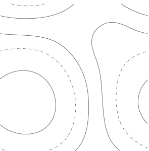
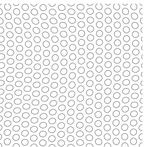
Figure 6: State resulting from the long-wave instability $\sigma_{1}>0$ ($\nu=2$, $\gamma=0.3$, $q=0.5$, $\mu-\mu_{H}=0.1$, $L=250$). a) The dashed and solid lines mark the zero contour lines of the real and imaginary part of the oscillation amplitude ${\cal H}$. b) Reconstruction of the hexagonal pattern from a), with $\tilde{q}_{c}=0.4$

In addition to the long-wave instabilities a short-wave instability appears for larger values of the hexagon wavenumber $q$. This instability is induced by the short-wave instability of the steady hexagons [25] and cannot be studied with the amplitude-phase equations (7), (2). As $\mu$ is increased above $\mu_{H}$, the oscillating hexagons arise through a Hopf bifurcation off the steady hexagons. Since that bifurcation occurs at zero wavenumber it affects the long-wave properties of the system and we expect that the long-wave stability limits of the steady and of the oscillating hexagons differ qualitatively. The effect of the Hopf bifurcation on short-wave instabilities, on the other hand, should vanish as the amplitude of the oscillations goes to 0. Thus, we expect a continuous transition from the short-wave instability of the steady to that of the oscillating hexagons as the line $\mu=\mu_{H}$ is crossed. In order to check this, we numerically determine the short-wave instability of the oscillating hexagons and compare it with the stability results for the steady hexagons, as obtained from solving the sixth-order dispersion relation associated with Eq. (2) [25]. The transition is indeed continuous, as expected. The stability region of the oscillating hexagons turns out to be reduced as compared to that of the steady hexagons when $\mu$ is increased (see Fig. 7).

Figure 7: Short-wave stability of oscillating hexagons (stars) and steady hexagons (circles) for the same parameters as in Fig. 4a ($\nu=2$, $\gamma=0.5$). Solid line: Hopf bifurcation of steady hexagons.

If the noise added to the oscillating hexagons is sufficiently large, different dynamics may arise even in the parameter range in which the oscillating hexagons are linearly stable. As indicated earlier, within the framework of the three coupled Ginzburg-Landau equations (2) one obtains for the parameters in the CGLE (16) values for which a persistent chaotic state exists while the plane waves are linearly stable. A detailed study of the chaotic state, which is characterized by the creation and annihilation of defects, comparing its description using the coupled Ginzburg-Landau equations (2), the amplitude-phase equations (7,2), and the single CGLE (16) has been presented elsewhere [19]. One of the main results of that study is the observation that this system is one of the few in which the defect chaos of the CGLE should be accessible experimentally.

5 Conclusions

In this paper we have studied the effect of a breaking of the chiral symmetry on systems that exhibit hexagon patterns. Classic examples of such systems are non-Boussinesq and surface-tension-driven convection with rotation. We have focused on the dynamics of the oscillating hexagons that arise in a Hopf bifurcation due to the rotation. In the vicinity of this secondary Hopf bifurcation the oscillating hexagons are described by a single complex Ginzburg-Landau equation (CGLE) coupled to the two phases of the underlying hexagons. The resulting amplitude-phase equations have certain similarities with those describing the secondary Hopf bifurcation observed in rectangle patterns in electro-convection in nematics [23].

Like the CGLE, the amplitude-phase equations support homogeneously oscillating solutions as well as traveling waves. In the latter, the coupling to the phases induces a drift of the hexagons in a direction that is typically oblique to the propagation direction of the traveling waves. The stability analysis of the oscillating and the traveling hexagons reveal two types of long-wave instabilities, one occurring when the hexagons are far away from the band-center, the other for high enough rotation rate. Even in this latter case, in finite systems there is always a stable region close to the band-center, its size depending on the size of the system. In both cases, the instabilities appear to be supercritical, giving rise to a spatially modulated oscillating hexagonal pattern.

Although there is always a region in which the homogeneously oscillating hexagons are linearly stable within the three coupled Ginzburg-Landau equations, they are in fact only meta-stable. Sufficiently large perturbations induce a transition to a state of defect chaos described by the CGLE [19]. There is always bistability between the chaotic state and the ordered oscillations. In that respect the chaotic state resembles spiral-defect chaos as it is observed in Rayleigh-Bénard convection at low Prandtl numbers [37]. As in that system the ordered states can presumably only be obtained by carefully controlled initial conditions. Rotating hexagon convection appears to be the first system in which the defect chaotic regime of the CGLE should be accessible experimentally.

From numerical simulations of the amplitude equations (2) it has been shown that a transition between defect-chaos and a frozen vortex state occurs for wavenumbers far away from the band-center [19]. This transition happens when the asymptotic plane waves emitted by the spirals become absolutely unstable. Therefore, the stability results for the traveling wave solution are relevant in order to determine the range of existence of the chaotic state found in [19]. A complete treatment of this point would involve the determination of the asymptotic wavenumber $k_{\infty}$ for the waves emitted by the spiral solutions of the coupled amplitude-phase equations.

In the present work, we have studied the system close to the bifurcation point, where analytical results can be obtained. However, far away from the Hopf bifurcation, a number of interesting effects are expected. One is related to the strength of the chiral symmetry breaking. To leading order in the perturbation expansion, the usual single CGLE is obtained, which is chirally symmetric. The breaking of the chiral symmetry appears only through the coupling with the phase, and vanishes at the band-center. For larger values of the oscillation amplitude, higher-order terms breaking the chiral symmetry of the CGLE are expected. This leads to an asymmetry between defects with opposite topological charge [38], with one type of spirals becoming dominant in the frozen vortex state. The asymptotic wavenumber, as well as the onset of absolute instability, becomes different for positively and negatively charged spirals, and the transition to the defect chaotic regime is different than in the chirally symmetric case [38]. We expect that this effect of the chiral symmetry breaking can be observed with Eqs. (2), as the control parameter is increased above the Hopf bifurcation.

Another open question is the relation of the limit cycle corresponding to the oscillating hexagons with the heteroclinic orbit arising in the Küppers-Lortz instability of rolls. As the limit cycle approaches the mixed-mode solutions, the harmonic oscillations are transformed into a switching between the three roll modes making up the hexagons similar to the dynamics arising in the Küppers-Lortz regime. This suggest a connection between the domain chaos found in these systems and the regular and disordered states discussed in this paper. However, it is worth emphasizing that in the defect chaos regime described in [19], the orientation of the hexagons is well defined and what is spatially chaotic is the modulation of the amplitudes that compose the hexagon pattern. In the Küppers-Lortz regime, on the other hand, patches of rolls with arbitrary orientation are possible, resulting in a state with an isotropic Fourier spectrum. Thus, a quantitative comparison between both states is not possible with Ginzburg-Landau equations such as (2) and generalized Swift-Hohenberg models must be considered [39].

Acknowledgments

We gratefully acknowledge interesting discussions with F. Sain and M. Silber. The numerical simulations were performed with a modification of a code by G.D. Granzow. This work was supported by D.O.E. Grant DE-FG02-G2ER14303 and NASA Grant NAG3-2113.

Appendix A Derivation of the Amplitude-Phase Equations

At the Hopf bifurcation, the hexagon solution (2) becomes $R_{H}=1/(\nu-1)$. We will consider perturbations around this solution, both in amplitude and phase:

$$A_{i}=(R_{H}+r_{i})e^{i{\bf q}_{i}\cdot{\bf x}+\phi_{i}+\Phi},$$ (52)

where $\Phi=\phi_{1}+\phi_{2}+\phi_{3}$ is the global phase of the hexagons and the three phases $\phi_{i}$ can be written as

$$\phi_{1} = \phi_{x},$$

$$\phi_{2} = -\phi_{x}/2+\sqrt{3}\phi_{y}/2,$$

$$\phi_{3} = -\phi_{x}/2-\sqrt{3}\phi_{y}/2,$$

where we have defined the phase vector $\vec{\phi}=(\phi_{x},\phi_{y})$, with $\phi_{x}$ and $\phi_{y}$ related to translations of the pattern in the x- and y-directions.

For the perturbations of the modulus $r_{i}$ there are three eigenvalues, one real, $\sigma_{1}=-2R^{2}(1+2\nu)+R$, corresponding to an eigenvector with $r_{1}=r_{2}=r_{3}$ and a complex conjugate pair, $\sigma_{2,3}=-2R^{2}(1-\nu)-2R\pm 2\sqrt{3}R^{2}\gamma i$, whose real part vanishes at $\mu=\mu_{H}$. The corresponding eigenvector satisfies $r_{3}=e^{2\pi i/3}r_{2}=e^{4\pi i/3}r_{1}$.

Taking this into account, we consider the expansion:

$$r_{1} = \epsilon r+\left[(-\frac{1}{2}+i\frac{\sqrt{3}}{2})(\sqrt{\epsilon}{\cal H}e^{i\omega t}+\epsilon({\cal H}_{10}+\overline{\cal H}_{12}e^{-2i\omega t}))+c.c.\right],$$

$$r_{2} = \epsilon r+\left[(-\frac{1}{2}-i\frac{\sqrt{3}}{2})(\sqrt{\epsilon}{\cal H}e^{i\omega t}+\epsilon({\cal H}_{10}+\overline{\cal H}_{12}e^{-2i\omega t}))+c.c.\right],$$

$$r_{3} = \epsilon r+\left[(\sqrt{\epsilon}{\cal H}e^{i\omega t}+\epsilon({\cal H}_{10}+\overline{\cal H}_{12}e^{-2i\omega t}))+c.c.\right],$$

$$\phi_{x} = \sqrt{\epsilon}\phi_{x}+\epsilon(\phi_{x1}e^{i\omega t}+c.c.),$$

$$\phi_{y} = \sqrt{\epsilon}\phi_{y}+\epsilon(\phi_{y1}e^{i\omega t}+c.c.),$$

$$\Phi = \epsilon(\Phi_{1}e^{i\omega t}+c.c.).$$

We also assume that the resulting state evolves on long time and space scales, specifically: $\partial_{t}\sim{\cal O}(\epsilon)$, $\nabla\sim{\cal O}(\epsilon^{1/2})$. Substituting the former expressions into Eq. (2), at ${\cal O}(\epsilon^{1/2})$ the linear problem is recovered, giving the value for the critical frequency: $\omega_{H}=-2\sqrt{3}R_{H}^{2}\gamma$.

At ${\cal O}(\epsilon)$ an algebraic relation between the slaved and the marginal modes is obtained:

$$\phi_{x1} = \frac{q}{2R_{H}}(\sqrt{3}+i)(\partial_{x}{\cal H}-i\partial_{y}{\cal H}),$$ (53)

$$\phi_{y1} = -\frac{qi}{2R_{H}}(\sqrt{3}+i)(\partial_{x}{\cal H}-i\partial_{y}{\cal H}),$$ (54)

$$\Phi_{1} = \frac{q}{2R_{H}(3R_{H}+i\omega_{H})}(\sqrt{3}i-1)(\partial_{x}{\cal H}+i\partial_{y}{\cal H}),$$ (55)

$$r = \frac{1}{3R_{H}(1+2R_{H})}\left[\mu R_{H}-(1+6R_{H})|{\cal H}|^{2}-qR_{H}\nabla\cdot\vec{\phi}\right],$$ (56)

$${\cal H}_{10} = -\frac{qR_{H}}{4\omega_{H}}(\sqrt{3}i+1)\left[\partial_{x}\phi_{y}+\partial_{y}\phi_{x}+i(\partial_{x}\phi_{x}-\partial_{y}\phi_{y})\right],$$ (57)

$${\cal H}_{12} = \frac{1}{6}\left(1+\frac{8i}{\omega_{H}}\right){\cal H}^{2}.$$ (58)

At ${\cal O}(\epsilon^{3/2})$ we obtain a solvability condition for ${\cal H}$ and $\vec{\phi}$:

$$\partial_{t}{\cal H} = \mu{\cal H}+\frac{1}{2}\nabla^{2}{\cal H}-q{\cal H}\nabla\cdot\vec{\phi}-\left(1+6R_{H}-\frac{2\omega_{H}i}{R_{H}}\right)r{\cal H}$$ (59)

$$-\frac{1}{R_{H}^{2}}\left[3R_{H}(1+2R_{H})-\frac{\omega i}{2}\right]|{\cal H}|^{2}{\cal H}+\left(8-\frac{\omega i}{R_{H}}\right)\overline{\cal H}{\cal H}_{12}$$

$$+\frac{R_{H}q}{4}(1+\sqrt{3}i)[\partial_{x}\phi_{x1}-\partial_{y}\phi_{y1}+i(\partial_{x}\phi_{y1}+\partial_{y}\phi_{x1})]$$

$$+\frac{R_{H}q}{2}(\sqrt{3}i+1)(\partial_{x}\Phi_{1}-i\partial_{y}\Phi_{1}),$$

$$\partial_{t}\phi_{x} = \frac{1}{4}\nabla^{2}\phi_{x}+\frac{1}{2}\partial_{x}(\nabla\cdot\vec{\phi})+\frac{2q}{R_{H}}\partial_{x}r$$ (60)

$$+\frac{q}{2R_{H}}\left[(\sqrt{3}i-1)(\partial_{x}{\cal H}_{10}-i\partial_{y}{\cal H}_{10})+c.c.\right]$$

$$+\frac{\omega}{4R_{H}}\left[(i-\sqrt{3})\overline{\cal H}(\phi_{x1}+i\phi_{y1})+c.c.\right]$$

$$-\frac{1}{2R_{H}}\left[(1+\sqrt{3}i)(3R_{H}-\omega i)\overline{\cal H}\Phi_{1}+c.c.\right],$$

$$\partial_{t}\phi_{y} = \frac{1}{4}\nabla^{2}\phi_{y}+\frac{1}{2}\partial_{y}(\nabla\cdot\vec{\phi})+\frac{2q}{R_{H}}\partial_{y}r$$ (61)

$$+\frac{q}{2R_{H}}\left[(\sqrt{3}+i)(\partial_{x}{\cal H}_{10}-i\partial_{y}{\cal H}_{10})+c.c.\right]$$

$$-\frac{\omega}{4R_{H}}\left[(1+\sqrt{3}i)\overline{\cal H}(\phi_{x1}+i\phi_{y1})+c.c.\right]$$

$$-\frac{1}{2R_{H}}\left[(\sqrt{3}-i)(3R_{H}-\omega i)\overline{\cal H}\Phi_{1}+c.c.\right].$$

Substituting the expressions of the slaved modes into the former equations we obtain the amplitude-phase equations (7), (2).

Appendix B Nonlinear Gradient Terms

If we retain in the Ginzburg-Landau equations (2) the nonlinear gradient terms that express the dependence of the quadratic coupling term on the hexagon wavenumber [25] we obtain

$$\partial_{t}A_{1} = \mu A_{1}+({\bf{n}}_{1}\cdot\nabla)^{2}A_{1}+\overline{A}_{2}\overline{A}_{3}-A_{1}|A_{1}|^{2}$$ (62)

$$-(\nu+\gamma)A_{1}|A_{2}|^{2}-(\nu-\gamma)A_{1}|A_{3}|^{2}$$

$$+i(\alpha_{1}+\tilde{\alpha})\overline{A}_{2}({\bf{n}}_{3}\cdot\nabla)\overline{A}_{3}+i(\alpha_{1}-\tilde{\alpha})\overline{A}_{3}({\bf{n}}_{2}\cdot\nabla)\overline{A}_{2}$$

$$+i\alpha_{2}\left(\overline{A}_{2}(\mbox{\boldmath$\tau$}_{3}\cdot\nabla)\overline{A}_{3}-\overline{A}_{3}(\mbox{\boldmath$\tau$}_{2}\cdot\nabla)\overline{A}_{2}\right).$$

For the amplitude-phase equations (7), (2) we obtain then the coefficients:

$$\alpha=1+2q\alpha_{1},$$

$$R_{H}=\frac{\alpha}{\nu-1},$$

$$\epsilon_{c}=\frac{\alpha^{2}(2+\nu)}{(\nu-1)^{2}}+q^{2}=R_{H}(3R_{H}+\alpha)+q^{2},$$

$$v=3R_{H}(\alpha+2R_{H}),$$

$$\omega_{H}=2\sqrt{3}\gamma R_{H}^{2},$$

$$\delta_{1}=\frac{2\alpha R_{H}}{v}-\frac{2i\omega_{H}}{v},$$

$$\delta_{2}=\frac{2\alpha R_{H}q}{v}+\frac{4R_{H}^{2}\alpha_{1}(3R_{H}+\alpha)}{v}-\frac{2i\omega_{H}(q-R_{H}\alpha_{1})}{v},$$

$$\xi=\frac{1}{2}-\frac{R_{H}(R_{H}\alpha_{1}+q)}{9R_{H}^{2}\alpha^{2}+\omega_{H}^{2}}[\frac{\sqrt{3}}{2}\tilde{\alpha}\omega_{H}+3\alpha(q+\frac{R_{H}}{2}(\alpha_{1}-\sqrt{3}\alpha_{2}))]-\frac{\sqrt{3}R_{H}q\tilde{\alpha}}{\omega_{H}}$$

$$\hskip 19.91684pt-\frac{i(R_{H}\alpha_{1}+q)}{9R_{H}^{2}\alpha^{2}+\omega_{H}^{2}}\left[\omega_{H}q+\frac{R_{H}}{2}[\omega_{H}(\alpha_{1}-\sqrt{3}\alpha_{2})-3\sqrt{3}R_{H}\alpha\tilde{\alpha}]\right]-\frac{iq^{2}}{\omega_{H}}$$

$$\hskip 19.91684pt+\frac{iR_{H}^{2}}{4\omega_{H}}\left[(\alpha_{1}+\sqrt{3}\alpha_{2})^{2}+3\tilde{\alpha}^{2}\right]$$

$$\rho=\frac{8\alpha(3R_{H}+\alpha)}{v}-\frac{4i\omega_{H}(\alpha+4R_{H})}{R_{H}v}-\frac{32i\alpha^{2}}{3\omega_{H}},$$

$$D_{\bot}=\frac{1}{4}-\frac{\sqrt{3}R_{H}q\tilde{\alpha}}{\omega_{H}},$$

$$D_{\|}=\frac{1}{2}-\frac{R_{H}\alpha_{1}-q}{v}\left[R_{H}(\alpha_{1}-\sqrt{3}\alpha_{2})-2q\right],$$

$$D_{\times_{1}}=\frac{q^{2}}{\omega_{H}}-\frac{R_{H}^{2}}{4\omega_{H}}\left[(\alpha_{1}+\sqrt{3}\alpha_{2})^{2}+3\tilde{\alpha}^{2}\right],$$

$$D_{\times_{2}}=\frac{\sqrt{3}R_{H}\tilde{\alpha}}{v}(R_{H}\alpha_{1}-q),$$

$$\alpha=-\frac{\alpha+6R_{H}}{R_{H}v}[2q+R_{H}(\sqrt{3}\alpha_{2}-\alpha_{1})]+\frac{18\alpha^{2}R_{H}^{3}\alpha_{1}-2\omega_{H}^{2}q}{R_{H}^{2}(9R_{H}^{2}\alpha^{2}+\omega_{H}^{2})},$$

$$\beta_{1}=\frac{6\omega_{H}\alpha(q+R_{H}\alpha_{1})}{R_{H}(9R_{H}^{2}\alpha^{2}+\omega_{H}^{2})}+\frac{\sqrt{3}\tilde{\alpha}}{v}(\alpha+6R_{H}),$$

$$\beta_{2}=\frac{6\omega_{H}\alpha(q+R_{H}\alpha_{1})}{R_{H}(9R_{H}^{2}\alpha^{2}+\omega_{H}^{2})}+\frac{\sqrt{3}\tilde{\alpha}}{R_{H}},$$

$$\eta=\frac{[9R_{H}^{2}\alpha^{2}(2q-R_{H}(\alpha_{1}+\sqrt{3}\alpha_{2}))-R_{H}\omega_{H}^{2}(3\alpha_{1}+\sqrt{3}\alpha_{2})]}{R_{H}^{2}(9R_{H}^{2}\alpha^{2}+\omega_{H}^{2})}.$$

B.1 Comparison with the CGLE

After rescaling we obtain the values for the coefficients of the CGLE (16). The coefficient $b_{3}$ now becomes:

$$b_{3}=\frac{2|\omega_{H}|R_{H}\alpha(\alpha+3R_{H})}{\omega_{H}^{2}(\alpha+4R_{H})+8R_{H}^{2}\alpha^{2}(\alpha+2R_{H})}.$$ (63)

For $q\neq 0$ the maximum value of $b_{3}$ is:

$$b^{max}_{3}=\frac{\alpha+3R_{H}}{\sqrt{8(\alpha+2R_{H})(\alpha+4R_{H})}},$$ (64)

and the limits for small and large $R_{H}$ are the same as in (18), even if now $b_{3}$ depends on $q$ (through $\alpha=1+2q\alpha_{1}$). At the band-center $b_{3}$ becomes the same as (18).

The expression for $b_{1}$ is quite involved. At the band-center it reduces to:

$$b_{1}=\frac{(9R_{H}^{2}+\omega_{H}^{2})[(\alpha_{1}+\sqrt{3}\alpha_{2})^{2}+3\tilde{\alpha}^{2}]+2\omega_{H}\alpha_{1}[\omega_{H}(\sqrt{3}\alpha_{2}-\alpha_{1})+3\sqrt{3}R_{H}\tilde{\alpha}]}{2\omega_{H}(9R_{H}^{2}+\omega_{H}^{2}-\alpha_{1}R_{H}^{2}[3R_{H}(\alpha_{1}-\sqrt{3}\alpha_{2})+\sqrt{3}\tilde{\alpha}\omega_{H}])}.$$ (65)

An important change occurs with respect to the decoupling of the amplitude-phase equation. For $\alpha_{1}\neq 0$ the amplitude and the phases do not decouple anymore. It would require $\delta_{2r}=0$, $\delta_{2i}=0$. From the latter we obtain $q=R_{H}\alpha_{1}$, while the former implies

$$q=\frac{1}{4\alpha_{1}}\left[-(1+4R_{H}\alpha_{1}^{2})\pm\sqrt{(1-4R_{H}\alpha_{1})^{2}-48R_{H}^{2}\alpha_{1}^{2}}\right].$$ (66)

The only real solution for both conditions is $\alpha_{1}=0$.

References

- [1] G. Küppers and D. Lortz, J. Fluid Mech. 35, 609 (1969).
- [2] G. Küppers, Phys. Lett. A 32, 7 (1970).
- [3] F. Busse and K. Heikes, Science 208, 173 (1980).
- [4] F. Zhong, R. Ecke, and V. Steinberg, Physica D 51, 596 (1991).
- [5] F. Zhong and R. Ecke, Chaos 2, 163 (1992).
- [6] L. Ning and R. Ecke, Phys. Rev. E 47, 3326 (1993).
- [7] Y. Hu, R. Ecke, and G. Ahlers, Phys. Rev. Lett. 74, 5040 (1995).
- [8] Y. Hu, W. Pesch, G. Ahlers, and R. Ecke, Phys. Rev. E 58, 5821 (1998).
- [9] H. Xi, J. Gunton, and G. Markish, Physica A 204, 741 (1994).
- [10] Y. Tu and M. Cross, Phys. Rev. Lett. 69, 2515 (1992).
- [11] M. Fantz, R. Friedrich, M. Bestehorn, and H. Haken, Physica D 61, 147 (1992).
- [12] M. Neufeld, R. Friedrich, and H. Haken, Z. Phys. B 92, 243 (1993).
- [13] T. Clune and E. Knobloch, Phys. Rev. E 47, 2536 (1993).
- [14] M. Cross, D. Meiron, and Y. Tu, Chaos 4, 607 (1994).
- [15] Y. Ponty, T. Passot, and P. Sulem, Phys. Fluids 9, 67 (1997).
- [16] J. Swift, in Contemporary Mathematics Vol. 28 (American Mathematical Society, Providence, 1984), p. 435.
- [17] A. Soward, Physica D 14, 227 (1985).
- [18] J. Millán-Rodríguez et al., Phys. Rev. A 46, 4729 (1992).
- [19] B. Echebarria and H. Riecke, preprint, patt-sol/9912002. .
- [20] P. Coullet and G. Iooss, Phys. Rev. Lett. 64, 866 (1990).
- [21] F. Daviaud et al., Physica D 55, 287 (1992).
- [22] H. Sakaguchi, Prog. Theor. Phys. 89, 1123 (1993).
- [23] B. Janiaud, H. Kokubo, and M. Sano, Phys. Rev. E 47, 2237 (1993).
- [24] S. Chandrasekhar, Hydrodynamic and Hydromagnetic Stability (Clarendon, Oxford, 1961).
- [25] B. Echebarria and H. Riecke, to appear in Physica D, patt-sol/9906008 .
- [26] J. Lauzeral, S. Metens, and D. Walgraef, Europhys. Lett. 24, 707 (1993).
- [27] R. Hoyle, Appl. Math. Lett. 9, 81 (1995).
- [28] H. Chaté and P. Manneville, Physica A 224, 348 (1996).
- [29] P. Manneville and H. Chaté, Physica D 96, 30 (1996).
- [30] G. Grinstein, C. Jayaprakash, and R. Pandit, Physica D 90, 96 (1996).
- [31] R. Montagne, E. Hernández-García, and M. S. Miguel, Physica D 96, 47 (1996).
- [32] R. Montagne, E. Hernández-García, A. Amengual, and M. S. Miguel, Phys. Rev. E 56, 151 (1997).
- [33] A. Torcini, Phys. Rev. Lett. 77, 1047 (1996).
- [34] A. Torcini, H. Frauenkron, and P. Grassberger, Phys. Rev. E 55, 5073 (1997).
- [35] S. Popp, O. Stiller, I. Aranson, and L. Kramer, Physica D 84, 398 (1995).
- [36] T. Benjamin and J. Feir, J. Fluid Mech. 27, 417 (1967).
- [37] R. Cakmur, D. Egolf, B. Plapp, and E. Bodenschatz, Phys. Rev. Lett. 79, 1853 (1997).
- [38] K. Nam, E. Ott, M. Gabbay, and N. Guzdar, Physica D 118, 69 (1998).
- [39] F. Sain and H. Riecke, Physica D, submitted .