On the relation between coupled map lattices
and kinetic Ising models

Abstract

A spatially one dimensional coupled map lattice possessing the same symmetries as the Miller Huse model is introduced. Our model is studied analytically by means of a formal perturbation expansion which uses weak coupling and the vicinity to a symmetry breaking bifurcation point. In parameter space four phases with different ergodic behaviour are observed. Although the coupling in the map lattice is diffusive, antiferromagnetic ordering is predominant. Via coarse graining the deterministic model is mapped to a master equation which establishes an equivalence between our system and a kinetic Ising model. Such an approach sheds some light on the dependence of the transient behaviour on the system size and the nature of the phase transitions.

I Introduction

Since the middle of the seventies the investigation of deterministic chaos has become one of the prominent fields in science, especially physics. A lot of knowledge has been gained since that time, in particular for low degree of freedom systems [1], and a whole machinery of tools has been developed for the diagnostics of chaotic motion. We just mention Lyapunov exponents and fractal dimensions as the most popular quantities. Parallel to these developments the question has been raised to which extent the number of degrees of freedom enters the business. Unfortunately, much less progress has been achieved in this direction. Only few results are available and most of them are bound to the investigation of model systems. Within that context coupled map lattices (CMLs) have been introduced at the end of the eighties as a widely studied model class [2, 3]. In such models local chaos is generated by a chaotic map which is placed at each site of a simple lattice. Spatial aspects are introduced by coupling these local units and special emphasis is on the limit of large lattice size where the dynamics becomes high dimensional.

There is just one class of many degree of freedom systems which is fairly well understood, namely statistical mechanics at and near thermal equilibrium. Unfortunately, the systems studied in the field of space time chaos are often far from equilibrium so that the tools of equilibrium statistical mechanics may fail. Nevertheless, the reduction to relevant degrees of freedom, sometimes called coarse graining, may be equally successful in both areas. By elimination of irrelevant degrees of freedom one maps the microscopic deterministic equation of motion to a stochastic model where the noise captures the irrelevant information. Such a concept, well developed in equilibrium statistical mechanics, has also been used in nonlinear dynamical systems; introductions can be found on the textbook level [4]. In a rigorous approach coarse graining is performed by suitable partitions of the phase space and there are results for particular coupled map lattices available (cf. [5, 6]). Unfortunately, such schemes are limited to some perturbative regime and are technically extremely difficult to apply. Henceforth, sometimes more physically motivated coarse grainings are used [7] relaxing the amount of rigour a little bit.

The just mentioned statistical methods become especially relevant in the study of phase transitions in CMLs [8]. Qualitative changes in the dynamical behaviour may be related to phase transition like scenarios in the corresponding coarse grained description. Prominent examples for such phenomena occur in the models introduced by Sakaguchi [9] and Miller and Huse [10]. To keep the paper self contained and as a motivation for the construction of our model we shortly review basic features of the latter model.

In order to mimic a phase transition in a two dimensional Ising model, the chaotic antisymmetric map depicted in figure 1 was placed onto a square lattice and coupled to its four nearest neighbours

$$x_{i\,j}^{t+1}:=\left(1-\epsilon\right)\phi\left(x_{i\,j}^{t}\right)+\frac{\epsilon}{4}\sum_{k,l=\pm 1}\phi\left(x_{i+k\,\,j+l}^{t}\right)\quad.$$ (1)

Performing a coarse graining according to the sign of the phase space variables

$$\alpha_{i\,j}^{t}=\left\{\begin{array}[]{ l @{\, ,\quad\; \mbox{if} \quad x_{i\, j}^t} r}+1\hfil\,,\quad\;\mbox{if}\quad x_{i\,j}^{t&\geq 0\\ -1\hfil\,,\quad\;\mbox{if}\quad x_{i\,j}^{t&<0\end{array}\right.}}$$ (2)

numerical simulations indicate a phase transition if the coupling strength exceeds a critical value $\epsilon_{crit.}\approx 0.82$ (cf. figure 1). Extensive numerical simulations indicate [11] that the phase transition is continuous. However, it is doubtful whether the transition belongs to the Ising universality class, because the results for the critical exponents are inconclusive. In particular, their values depend on whether the CML is updated synchronously or asynchronously. One can summarise that the phase transition of the Miller Huse model is still far from being understood, in particular since no quantitative description of the spin dynamics could be derived. In order to reach some progress in this direction we here introduce and investigate a slightly different model system with analytical methods.

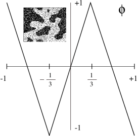
FIG. 1.: The single site map $\phi$ of the Miller Huse model. The inset shows a typical pattern for $\epsilon>\epsilon_{crit.}$ (white/black $\alpha_{i\,j}=\pm 1$).

Section II introduces our model as well as the setup of the perturbation expansion. For the latter purpose transitions between sets of a suitable partition are defined. These transitions are studied in detail in section III. Herewith, the bifurcation diagram of our model will be developed in section IV and analytical expressions for the bifurcation lines are calculated in perturbation theory. Section V is devoted to a systematic coarse graining of the dynamics on the basis of the just mentioned partition. On that level the dynamics is described in terms of a master equation which corresponds to a particular class of kinetic Ising models. It constitutes the basis for the investigation of the transient behaviour in section VI. Finally, the main results of this work are summarised. The appendices are concerned with parts of the perturbation expansion, but more details can be found in [12].

II The model

Let us first consider the single site map. It consists of a deformed antisymmetric tent map $f_{\delta}$, which is linear on three subintervals of $[-1,\,1]$

$$f_{{\delta}}(x):=\left\{\begin{array}[]{r @{\; , \; \;{\rm if} \quad\; x \in\,} l}-2-x/a&[-1,-a]\\ x/a&(-a,a)\\ 2-x/a&[a,1]\end{array}\right.\;,\quad a:=\frac{1}{2-{\delta}}\quad.$$ (3)

Because of $f_{{\delta}}(1)=\delta$ the parameter $\delta$ determines whether transitions between the intervals $[-1,0]=:J(-1)$ and $[0,1]=:J(+1)$ are possible. Note that the Miller Huse map is obtained as a special case, $\phi=f_{\delta=-1}$. The introduction of $a$ in eq. (3) ensures that the modulus of the derivative of $f_{{\delta}}$ is constant on the whole interval. Figure 2 shows the function $f_{\delta}$ for small positive and negative $\delta$. For $\delta\geq 0$ the single site map has two coexisting attractors, the intervals $[-1,\,\delta]$ and $[\delta,\,1]$, whereas for $\delta<0$ only one attractor, the interval $[-1,\,1]$, is present.

FIG. 2.: The deformed antisymmetric tent map $f_{\delta}$.

The CML which is studied in this article is defined on a one dimensional lattice (chain) of length $N$. Nearest neighbours are coupled in a standard ”diffusive” way with periodic boundary conditions

$${\mathbf{T}}_{{\epsilon},{\delta}} : [-1,+1]^{N}\rightarrow[-1,+1]^{N}\;,$$ (4)

$$\left[\mathbf{T_{{\epsilon},{\delta}}({\mathbf{x}})}\right]_{i} := (1-{\epsilon})\,f_{{\delta}}(x_{i})+\frac{\epsilon}{2}\,(f_{{\delta}}(x_{i-1})+f_{{\delta}}(x_{i+1}))\quad.$$ (5)

The parameter $\epsilon$ denotes the coupling strength. Because of the single site map and the diffusive coupling the CML ${\mathbf{T}}_{{\epsilon},{\delta}}$ has the symmetry ${\mathbf{T}}_{{\epsilon},{\delta}}(-{\mathbf{x}})=-{\mathbf{T}}_{{\epsilon},{\delta}}({\mathbf{x}})$. Furthermore, translation invariance on the one dimensional lattice holds, because periodic boundary conditions have been imposed.

Since we are going to perform a perturbation theory with $\epsilon,\,|\delta|\ll 1$, we first consider the CML with $\epsilon=\delta=0$. In this case the model can be solved trivially. The non–deformed antisymmetric tent map $f_{0}$ has the two attractors $J(-1)=[-1,\,0]$ and $J(+1)=[0,\,1]$. Therefore, $N$ uncoupled maps $f_{0}$ have $2^{N}$ coexisting attractors, each one an $N$ dimensional cube of edge length one

$$I_{\bm{\alpha}}:=J({\alpha}_{1})\times J({\alpha}_{2})\times\dots\times J({\alpha}_{N})\;\quad.$$ (6)

We distinguish these cubes $I_{\bm{\alpha}}$ by an $N$ dimensional index vector $\bm{\alpha}=(\alpha_{1},\alpha_{2},\dots\alpha_{N})$ where $\alpha_{i}\in\{-1,\,+1\}$. The natural measure on each cube is the Lebesgue measure. As we will see these cubes become important building blocks of the perturbation theory and the starting point of a coarse grained description of the CML ${\mathbf{T}}_{{\epsilon},{\delta}}$.

From a dynamical systems point of view we are mainly interested in ergodic properties of the CML, i. e. the number of coexisting attractors and their location for given small parameters $\epsilon,\,\delta$. An important observation is that in the perturbative regime a typical orbit stays for many iterations within a cube $I_{\bm{\alpha}}$, before it possibly enters another cube $I_{\bm{\beta}}$. Therefore, in perturbation theory any attractor of the CML ${\mathbf{T}}_{{\epsilon},{\delta}}$ is a union of cubes $I_{\bm{\alpha}}$, if one neglects sets with volume ${\cal O}(\epsilon,\,\delta)$. Hence, the dynamics is sufficiently characterised by transitions $I_{\bm{\alpha}}\rightarrow I_{\bm{\beta}}$ between cubes.

Of course we have to be more definite with what we mean by a transition. In order that a phase space point can be mapped from a cube $I_{\bm{\alpha}}$ to a cube $I_{\bm{\beta}}$ ($\bm{\alpha}\neq\bm{\beta}$) the image of the former has to intersect the latter. Hence the overlap set

$$OV_{\bm{\alpha},\,\bm{\beta}}:={\mathbf{T}}_{{\epsilon},{\delta}}(I_{\bm{\alpha}})\cap I_{\bm{\beta}}$$ (7)

plays an important role. A necessary condition for a point to migrate from $I_{\bm{\alpha}}$ to $I_{\bm{\beta}}$ is a non–empty overlap set $OV_{\bm{\alpha},\,\bm{\beta}}$. Since in perturbation theory the set ${\mathbf{T}}_{{\epsilon},{\delta}}(I_{\bm{\alpha}})$ is a weakly deformed cube $I_{\bm{\alpha}}$, the set $OV_{\bm{\alpha},\,\bm{\beta}}$ can at most have a volume of size ${\cal O}(\epsilon,\,\delta)$. However, the condition on the overlap set is far from being sufficient because one has to ensure that typical orbits can reach this set upon their itinerary. For that purpose two additional conditions have to be imposed.

First, we have to ensure that points from the inner part of $I_{\bm{\alpha}}$ reach the overlap set. For that reason we consider the pre–images of $OV_{\bm{\alpha},\,\bm{\beta}}$ of various generation that are contained in $I_{\bm{\alpha}}$

$${\mathbf{T}}_{{\epsilon},{\delta}}^{-1}(OV_{\bm{\alpha},\,\bm{\beta}}) := \{{\mathbf{x}}\in I_{\bm{\alpha}}\;|\;{\mathbf{T}}_{{\epsilon},{\delta}}({\mathbf{x}})\in OV_{\bm{\alpha},\,\bm{\beta}}\}$$ (8)

$${\mathbf{T}}_{{\epsilon},{\delta}}^{-k}(OV_{\bm{\alpha},\,\bm{\beta}}) := \{{\mathbf{x}}\in I_{\bm{\alpha}}\;|\;{\mathbf{T}}_{{\epsilon},{\delta}}({\mathbf{x}})\in{\mathbf{T}}_{{\epsilon},{\delta}}^{-(k-1)}(OV_{\bm{\alpha},\,\bm{\beta}})\}\,,\hskip 17.07182ptk=2,3,\dots\quad.$$ (9)

For some finite $k$ the pre–image set ${\mathbf{T}}_{{\epsilon},{\delta}}^{-k}(OV_{\bm{\alpha},\,\bm{\beta}})$ should intersect the inner part of $I_{\bm{\alpha}}$, so that points from the inner part of $I_{\bm{\alpha}}$ can reach the overlap set $OV_{\bm{\alpha},\,\bm{\beta}}$.

The points of the set $OV_{\bm{\alpha},\,\bm{\beta}}$ are near the surface of the cube $I_{\bm{\beta}}$ within a distance of order ${\cal O}(\epsilon,\,\delta)$. The second condition demands that points from a subset of $OV_{\bm{\alpha},\,\bm{\beta}}$ with finite Lebesgue measure reach the inner part of the cube $I_{\bm{\beta}}$ directly under further iteration. The two conditions for a transition $I_{\bm{\alpha}}\rightarrow I_{\bm{\beta}}$ ensure that the transition is possible for a set of finite Lebesgue measure that is located in the inner part of $I_{\bm{\alpha}}$.

III Transitions in perturbation theory

In what follows we consider the CML ${\mathbf{T}}_{{\epsilon},{\delta}}$ for arbitrary but fixed lattice size $N$. We would like to know which transitions $I_{\bm{\alpha}}\rightarrow I_{\bm{\beta}}$ are possible for given parameters $\epsilon$, $\delta$. In the spirit of perturbation theory we confine ourselves to dominant transitions. Those are transitions where the cubes $I_{\bm{\alpha}}$ and $I_{\bm{\beta}}$ share an $(N-1)$ dimensional surface. Then, the volume of the overlap set $OV_{\bm{\alpha},\,\bm{\beta}}$ can be greater by a factor $1/\epsilon$ or $1/|\delta|$ in comparison to the case without a common surface. Consequently, the $N$ dimensional index vectors $\bm{\alpha}$ and $\bm{\beta}$ only differ in one component, the transition index $\alpha_{i}$. In such a transition $I_{\bm{\alpha}}\rightarrow I_{\bm{\beta}}$ the $x_{i}$ coordinate of the phase space orbit $\{{\mathbf{x}}^{t}\}$ changes its sign. Transitions of higher order in which two or more coordinates simultaneously change their sign will not be considered in this article, because their rates are smaller by a factor of the order ${\cal O}(\epsilon,\,\delta)$ in comparison to the dominant transitions.

In perturbation theory, for a dominant transition only the neighbouring indices of the transition index, $\alpha_{i-1}$ and $\alpha_{i+1}$, are relevant, because of the nearest neighbour interaction of the map ${\mathbf{T}}_{{\epsilon},{\delta}}$ (cf. eq. (5)). In addition, the influence of the two neighbouring coordinates $x_{i-1}$ and $x_{i+1}$ on the $x_{i}$ coordinate is predominant for a finite number of iterations, since interactions with lattice sites farther away are suppressed by the small coupling strength $\epsilon$. More precisely, within first order perturbation theory the overlap sets $OV_{\bm{\alpha},\,\bm{\beta}}$ and their pre–image sets can be approximated by the following product sets (cf. appendix A)

$$OV_{\bm{\alpha}\,,\bm{\beta}} = OV^{(3)}_{\alpha_{i-1}\,\alpha_{i}\,\alpha_{i+1},\beta_{i-1}\,\beta_{i}\,\beta_{i+1}}\times I^{(N-3)}_{\alpha_{1}\,\alpha_{2}\dots\alpha_{i-2}\,\alpha_{i+2}\dots\alpha_{N}}\;,$$ (10)

$${\mathbf{T}}_{\epsilon,\delta}^{-k}(OV_{\bm{\alpha},\,\bm{\beta}}) = \left[{\mathbf{T}}_{\epsilon,\delta}^{(3)}\right]^{-k}\left(OV^{(3)}_{\alpha_{i-1}\,\alpha_{i}\,\alpha_{i+1},\beta_{i-1}\,\beta_{i}\,\beta_{i+1}}\right)\;\times\;I^{(N-3)}_{\alpha_{1}\,\alpha_{2}\dots\alpha_{i-2}\,\alpha_{i+2}\dots\alpha_{N}}\,,\quad\quad k\geq 1\;\quad.$$ (11)

Here $OV^{(3)}_{\alpha_{i-1}\,\alpha_{i}\,\alpha_{i+1},\beta_{i-1}\,\beta_{i}\,\beta_{i+1}}$ denotes a three dimensional projection of the full overlap set which contains the coordinates $x_{i-1}$, $x_{i}$ and $x_{i+1}$, and ${\mathbf{T}}_{\epsilon,\delta}^{(3)}$ denotes the map lattice for $N=3$. The $(N-3)$ remaining coordinates are contained in the $(N-3)$ dimensional cube $I^{(N-3)}_{\alpha_{1}\,\alpha_{2}\dots\alpha_{i-2}\,\alpha_{i+2}\dots\alpha_{N}}$. Effectively, we have herewith reduced the transition in a map lattice of size $N$ to a transition in a map lattice of size three, because $(N-3)$ coordinates play only a spectator role. Put differently, the CML ${\mathbf{T}}_{{\epsilon},{\delta}}$ reaches already its full complexity for $N=3$, if one stays in the perturbative regime.

For symmetry reasons one can identify three different types of transitions $I_{\bm{\alpha}}\rightarrow I_{\bm{\beta}}$:

  Type (a):

the three indices $\alpha_{i-1}$, $\alpha_{i}$ and $\alpha_{i+1}$ are equal, e. g.

$\displaystyle I_{\dots,\,+1,\,+1,\,+1,\dots}\rightarrow I_{\dots,\,+1,\,-1,\,+1,\dots}\quad.$

  Type (b):

the two neighbouring indices $\alpha_{i-1}$ and $\alpha_{i+1}$ are different from each other, e. g.

$\displaystyle I_{\dots,\,-1,\,+1,\,+1,\dots}\rightarrow I_{\dots,\,-1,\,-1,\,+1,\dots}\quad.$

  Type (c):

the neighbouring indices $\alpha_{i-1}$ and $\alpha_{i+1}$ differ from the transition index $\alpha_{i}$, e. g.

$\displaystyle I_{\dots,\,+1,\,-1,\,+1,\dots}\rightarrow I_{\dots,\,+1,\,+1,\,+1,\dots}\quad.$

Transitions of type (c) are inverse to those of type (a).

Because of the conditions mentioned in the last section transitions are possible only if the deformation is small enough, $\delta<\delta_{crit.}\left(\epsilon\right)$. Within perturbation theory we obtain for the different critical values

$${\rm type\;(a)\,:}\;\delta_{a}=0\;,\quad{\rm type\;(b)\,:}\;\delta_{b}=-\frac{2\,\epsilon}{3}\;,\quad{\rm type\;(c)\,:}\;\delta_{c}=-\frac{4\,\epsilon}{3}\;\quad.$$ (12)

One might wonder why transitions (b) and (c) do not appear for negative $\delta$ above the critical value. The main reason is that despite of the existence of a non–empty overlap set trajectories do not reach this overlap since there exists a forbidden region in phase space called the ”blind volume”. Points belonging to the blind volume have no pre–images themselves. The blind volume is non–empty, since the map ${\mathbf{T}}_{\epsilon,\delta}$ is not surjective for finite coupling $\epsilon$. The actual calculation of critical $\delta$ values necessitates rather involved geometric constructions in phase space, since one must determine the location of the pre–image sets ${\mathbf{T}}_{\epsilon,\delta}^{-k}(OV_{\bm{\alpha},\,\bm{\beta}})$ in $I_{\bm{\alpha}}$. Hence, details are postponed to appendix B. The smaller the deformation parameter $\delta$, the more transitions become possible as can be guessed from the geometry of the map (cf. figure 2). On the other hand, increasing coupling constant $\epsilon$ inhibits transitions, since eventually only the transition of type (a) remains feasible for fixed negative $\delta$. Such an observation contradicts somehow the intuitive reasoning about a ”coupling” of lattice sites. The inhibition effect for transitions is caused by the existence of a ”blind volume” in the cube $I_{\bm{\alpha}}$ that grows with $\epsilon$ (cf. appendix B).

At this stage some remarks on the accuracy of our perturbative approach seem to be in order. Since we neglect transitions of higher order our arguments are not rigorous. In fact for a real proof the complete absence of such transitions must be shown. For the case of two coupled maps, $N=2$, such a step can be easily supplemented (cf. appendix C) and we infer that one might be able to perform similar but more involved computations in higher dimensional cases too. Nevertheless, even if these transitions are mathematically possible their effect may be small e.g. taking a time scale argument into account.

IV The bifurcation scenario

Eq. (12) determines four regions in the $\left(\epsilon,\,\delta\right)$ parameter plane where different transitions are possible (cf. figure 3). Crossing these lines a bifurcation occurs. Between different regions the number of coexisting attractors and their location change. Determining attractors in the strict mathematical sense just from the knowledge of the dominant transitions faces however some problems. For, neglecting sets with volume ${\cal O}(\epsilon,\,\delta)$ a union of cubes $A$, which an orbit can not leave through a dominant transition, is a candidate for an attractor. But, possibly an orbit can escape from this set through a transition of higher order in perturbation theory. Then the set $A$ would not be an attractor in a strict mathematical sense. However, one can put forward the following time scale argument: in perturbation theory transitions through which an orbit can leave $A$ occur on a rather large time scale in comparison to the relatively fast dominant transitions through which the orbit is pulled back to the set $A$ again. Because of this intermittent dynamics the set $A$ is a core region of a possibly bigger attractor, i. e.  the sets $A$ are the carriers of most of the natural measure of these attractors. For brevity we will call these sets $A$ ”attractors” in the following.

If we neglect sets with volume ${\cal O}(\epsilon,\,\delta)$ we can identify an attractor $A$ with a union of cubes $I_{\bm{\alpha}}$.

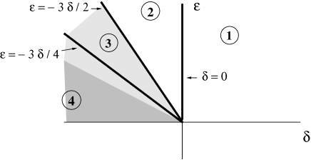
FIG. 3.: Diagrammatic view of the bifurcation diagram for the CML $\mathbf{T}_{{\epsilon},{\delta}}$ according to eq. (12). The numbers in the four parameter regions refer to the text. Gray–shading indicates the type of coupling in the corresponding kinetic Ising model, antiferromagnetic (light) resp. ferromagnetic (dark) (cf. section V).

  Region 1 ($\delta\geq 0$):

No transition $I_{\bm{\alpha}}\rightarrow I_{\bm{\beta}}$ is possible. Therefore, each cube $I_{\bm{\alpha}}$ is an attractor so that there are $2^{N}$ coexisting attractors.

  Region 2 ($-2\,\epsilon/3\leq\delta<0$):

Only transition type (a) is allowed. Hence, cubes $I_{\bm{\alpha}}$ are attractors such that $\bm{\alpha}$ does not contain three successive ”$+1$” or ”$-1$”. With a combinatorial argumentation one can show for that for long chains ($N\gg 1$) the number of coexisting attractors increases like $((1+\sqrt{5})/2)^{N}$.

  Region 3 ($-4\,\epsilon/3\leq\delta<-2\,\epsilon/3$):

To determine the attractors in this region, it seems necessary to anticipate the coarse graining of the CML ${\mathbf{T}}_{\epsilon,\delta}$ which will be discussed systematically in section V. Analogous to eq. (2) we can view the index vector $\bm{\alpha}$ of a cube $I_{\bm{\alpha}}$ as a spin chain of length $N$, where $+1$ and $-1$ are the possible spin states on each lattice site. In this way the three transition types (a), (b) and (c) translate into three different kinds of spin flips. For each spin chain one can define defects in the same way as in the antiferromagnetic Ising model. A defect (”$1$”) occurs, if two neighbouring spins are aligned, and no defect is present, if the spins point in opposite directions. Then, the just mentioned spin flips translate into a dynamics of defects.

  Type (a):

two adjacent defects annihilate each other, e. g.

$${\rm spin\;chain}\;\bm{\alpha}: \;\dots+1,\;+1,\;+1,\ldots\ldots\rightarrow\dots+1,\;-1,\;+1,\dots$$ (13)

$${\rm defects\;in}\;\bm{\alpha}: \;\;\dots\dots 1,\;\;\;\;1,\,\dots\dots\,\;\;\rightarrow\;\;\dots\dots\;0,\;\;\;\;\;0,\,\dots\dots$$ (14)

  Type (b):

one defect diffuses to a neighbouring lattice site, e. g.

$${\rm spin\;chain}\;\bm{\alpha}: \;\dots+1,\;+1,\;-1,\ldots\ldots\rightarrow\dots+1,\;-1,\;-1,\dots$$ (15)

$${\rm defects\;in}\;\bm{\alpha}: \;\;\dots\dots 1,\;\;\;\;0,\,\dots\dots\,\;\;\rightarrow\;\;\dots\dots\;0,\;\;\;\;\;1,\,\dots\dots$$ (16)

  Type (c):

two adjacent defects are generated simultaneously, e. g.

$${\rm spin\;chain}\;\bm{\alpha}: \;\dots+1,\;-1,\;+1,\ldots\ldots\rightarrow\dots+1,\;+1,\;+1,\dots$$ (17)

$${\rm defects\;in}\;\bm{\alpha}: \;\;\dots\dots 0,\;\;\;\;0,\,\dots\dots\,\;\;\rightarrow\;\;\dots\dots\;1,\;\;\;\;\;1,\,\dots\dots$$ (18)

For the determination of the attractors in the present parameter region we consider an orbit $\{{\mathbf{x}}^{t}\}$ of the CML which performs successive transitions $I_{\bm{\alpha}}\rightarrow I_{\bm{\beta}}$. Each transition changes the corresponding spin chain $\bm{\alpha}$ and its defects. Since transitions of type (c) are forbidden, defects can diffuse and annihilate in pairs only, and the number of defects decreases monotonically.

If the size of the system $N$ is even the chain contains an even number of defects. An orbit $\{{\mathbf{x}}^{t}\}$ migrates between cubes $I_{\bm{\alpha}}$, until all defects have annihilated each other. Then, the orbit can not execute any further transition of type (a) or (b). Therefore, there are two attractors, the cubes $I_{(\,{+1},{-1},{+1},{-1},\dots,{-1},{+1},{-1}\,)}$ and $I_{(\,{-1},{+1},{-1},{+1},\dots,{+1},{-1},{+1}\,)}$. Extensive numerical simulations indicate that for $N$ even each cube $I_{(\,{+1},{-1},{+1},{-1},\dots,{-1},{+1},{-1}\,)}$ and $I_{(\,{-1},{+1},{-1},{+1},\dots,{+1},{-1},{+1}\,)}$ constitutes an attractor in the strict sense, i. e. for $\delta>-4\,\epsilon/3$ no additional transition of higher order perturbation theory is present (cf. also appendix C)

For $N$ odd the number of defects in $\bm{\alpha}$ is odd. Consequently, at the end of the transient dynamics one defect remains. Since the defect can change its location via a transition of type (b), the attractor is the union of all $2\,N$ cubes $I_{\bm{\alpha}}$ for which $\bm{\alpha}$ contains a single ”$+1\;+1$” or ”$-1\;-1$” sequence.

Since in both cases the ratio of the volume of the attractor to the volume of its basin of attraction becomes very small for $N\gg 1$ one expects long transients to occur. Section VI is devoted to a more detailed study of the transient dynamics. Our argumentation has used the assumption that different transitions are not correlated. We will come back to this problem in the next section.

  Region 4 ($\delta<-4\,\epsilon/3$):

All three transition types are possible. Therefore an orbit $\{{\mathbf{x}}^{t}\}$ can visit every cube $I_{\bm{\alpha}}$, so that there emerges one attractor which encompasses all cubes.

V Coarse graining of the CML

Coarse graining the CML ${\mathbf{T}}_{\epsilon,\delta}$ one passes from orbits $\{{\mathbf{x}}^{t},\;t=0,\,1,\,2\dots\}$ in phase space to symbol or spin chains $\{\bm{\alpha}^{t},\;t=0,\,1,\,2\dots\}$. The spin chain $\bm{\alpha}^{t}$ just indicates the cube which contains the phase space point ${\mathbf{x}}^{t}$ at time $t$ (cf. eq. (2) ). If an orbit of the CML performs a transition $I_{\bm{\alpha}}\rightarrow I_{\bm{\beta}}$, the state of the spin chain changes from $\bm{\alpha}$ to $\bm{\beta}$. Since in perturbation theory an orbit typically circulates for many iterations within a cube $I_{\bm{\alpha}}$, the sequence $\{\bm{\alpha}^{t},\;t=0,\,1,\,2\dots\}$ has a constant value for long time before a spin flip occurs. Altogether, the CML is described by a stochastic spin dynamics. First we argue that the spin dynamics is Markovian for the following reasons:

• Two successive transitions $I_{\bm{\alpha}}\rightarrow I_{\bm{\beta}}$ and $I_{\bm{\beta}}\rightarrow I_{\bm{\gamma}}$ are uncorrelated. In the perturbative regime an orbit performs a highly chaotic motion within the cube $I_{\bm{\beta}}$ for many iterations before the transition to the cube $I_{\bm{\gamma}}$ occurs. Therefore, the memory of the preceding transition $I_{\bm{\alpha}}\rightarrow I_{\bm{\beta}}$ is lost.

• A transition $I_{\bm{\alpha}}\rightarrow I_{\bm{\beta}}$ is equally probable for each iteration step. For a transition the orbit point ${\mathbf{x}}^{t}$ must hit a characteristic set in the inner part of the cube $I_{\bm{\alpha}}$ which consists of pre–images of the overlap $OV_{\bm{\alpha},\,\bm{\beta}}$. During its stay within the cube $I_{\bm{\alpha}}$ the orbit is distributed uniformly within $I_{\bm{\alpha}}$, since for $\epsilon=\delta=0$ the natural measure on $I_{\bm{\alpha}}$ is the Lebesgue measure. Consequently, the probability for the orbit to hit the characteristic set is independent of time.

Since the spin dynamics is Markovian at least approximately, the probability $p_{\bm{\alpha}}(t)$ that the spin chain is in state $\bm{\alpha}$ at time $t$ obeys a master equation with transition probabilities $w\left(\bm{\beta}\,|\,\bm{\alpha}\right)$ for a spin flip $\bm{\alpha}\rightarrow\bm{\beta}$

$$p_{\bm{\alpha}}(t+1)=p_{\bm{\alpha}}(t)+\sum_{\bm{\beta}\neq\bm{\alpha}}\left[w(\bm{\alpha}\,|\,\bm{\beta})\cdot p_{\bm{\beta}}(t)-w(\bm{\beta}\,|\,\bm{\alpha})\cdot p_{\bm{\alpha}}(t)\right]\quad.$$ (19)

In perturbation theory three types of spin flips occur. As already stated above only a single spin flips during the elementary process $\bm{\alpha}\rightarrow\bm{\beta}$. From the study of the underlying CML ${\mathbf{T}}_{\epsilon,\delta}$ one can infer the following properties of the transition probabilities $w\left(\bm{\beta}\,|\,\bm{\alpha}\right)$.

• Because of the nearest neighbour coupling in eq. (5) and the direct product property (11) in the perturbative regime, the transition probabilities $w(\bm{\beta}\,|\,\bm{\alpha})$ depend on the three neighbouring spins only

  $$w(\bm{\beta}\,|\,\bm{\alpha})=w^{(3)}\left(\alpha_{i-1}\,\beta_{i}\,\alpha_{i+1}\;|\;\alpha_{i-1}\,\alpha_{i}\,\alpha_{i+1}\right)\;\quad,$$ (20)

  where $\alpha_{i}$ denotes the transition index. Hence the spin interaction is local.

• According to eq. (20) the transition probabilities $w\left(\bm{\beta}\,|\,\bm{\alpha}\right)$ do not depend on $N$. Therefore, they can be determined for small systems, e. g. $N=3$.

• Transitions of the three different types have probabilities $w_{a}$, $w_{b}$, and $w_{c}$, respectively, which depend on the parameters $\epsilon,\,\delta$. If $\delta$ is greater than the corresponding critical value in eq. (12), the respective transition probability strictly vanishes. Lowering $\delta$ the transition probability increases monotonously as can be shown by a rather subtle argument which uses the monotonous growth of the overlap set $OV_{\bm{\alpha},\,\bm{\beta}}$.

The dynamics resulting from the master equation (19) is almost trivial in parameter regions 1 and 2, since at most the spin flip of type (a) is possible. Regions 3 and 4 are more interesting, because at least two different spin flips occur. Since we are mainly interested in large systems, we confine ourselves to $N$ even in what follows.

In region 3 spin flips of type (a) and (b) are possible. On the coarse grained level the attractors $I_{(\,{+1},{-1},{+1},{-1},\dots,{-1},{+1},{-1}\,)}$ and $I_{(\,{-1},{+1},{-1},{+1},\dots,{+1},{-1},{+1}\,)}$ are viewed as the two ground states of the antiferromagnetic Ising model. Hence, the ergodic dynamics of the CML ${\mathbf{T}}_{\epsilon,\delta}$ corresponds to an antiferromagnetic Ising model at zero temperature. In parameter region 4 all three spin flips are possible. The (unique) stationary distribution of the master equation can be calculated with the ansatz that the weight of each state $\bm{\alpha}$ solely depends on the number of defects. The result

$$p^{stat}_{\bm{\alpha}}=c\left(\frac{w_{c}}{w_{a}}\right)^{\frac{1}{4}\sum_{i=1}^{N}\alpha_{i}\alpha_{i+1}}=\frac{1}{Z}\exp\left(\beta\,J\,\sum_{i=1}^{N}\alpha_{i}\alpha_{i+1}\right)$$ (21)

clearly can be cast into the form of a canonical distribution for a nearest neighbour coupled Ising chain. Here, $c$ and $Z$ denote the normalisation constants and for the temperature the relation

$$\beta\,J=\frac{1}{4}\log\left(\frac{w_{c}}{w_{a}}\right)$$ (22)

follows. Taking $J$ with modulus one the temperature depends on the ratio of the transition probabilities for generation and annihilation of two defects. It is finite throughout region 4. Ferromagnetic coupling, $J=+1$, is obtained for $(w_{c}/w_{a})>1$, whereas in the opposite case $(w_{c}/w_{a})<1$ antiferromagnetic coupling, $J=-1$, follows. Both cases are realized in the present parameter region, as can be seen in figure 3. Here, the transition probabilities $w_{a}$ and $w_{c}$ were obtained numerically by analysing the transitions of a very long orbit of the CML with $N=3$. Finally, it is easy to show that the stationary distribution (21) of eq. (19) obeys detailed balance

$\displaystyle w(\bm{\beta}\,|\,\bm{\alpha})\cdot p^{stat}_{\bm{\alpha}}=w(\bm{\alpha}\,|\,\bm{\beta})\cdot p^{stat}_{\bm{\beta}}\;,$

although the underlying CML describes a non–equilibrium process on the microscopic level.

VI Transient dynamics of the CML

As mentioned above the transient dynamics of the CML is most interesting in the parameter region 3 for which the attractors $I_{(\,{+1},{-1},{+1},{-1},\dots,{-1},{+1},{-1}\,)}$ and $I_{(\,{-1},{+1},{-1},{+1},\dots,{+1},{-1},{+1}\,)}$ have large basins of attraction for large $N$. The mean transient time $\langle T\rangle$ can be determined by averaging the time until an orbit reaches one of the two attractors over many random initial conditions, i.e. initial conditions distributed according to the Lebesgue measure. The numerical simulation indicates a quadratic increase with the system size

$$\langle T\rangle\propto N^{2}\quad\quad(N\gg 1)\quad.$$ (23)

Such a law can be understood from the coarse grained point of view. In parameter region 3 the spin flips of type (a) and (b) are allowed which cause the annihilation of two defects respectively the diffusion of one defect. Overall, the transient dynamics of the CML corresponds to a relaxation process towards one of the two ground states. Since diffusion is important for the relaxation the time scale grows with the second power of the length scale, i.e. the system size.

To be more definite and in order to derive eq. (23) formally we remind that the spin dynamics induced by the map lattice constitutes a kinetic Ising model with local spin flips. Models of these type have been introduced by R. J. Glauber in his celebrated article [13, 14]. So the coarse grained dynamics of the CML ${\mathbf{T}}_{\epsilon,\delta}$ belongs to a well–studied class of models. For the case of zero temperature, i. e. $w_{c}=0$, an exact analytical solution is available if an additional relation for the two remaining transition probabilities is imposed

$$w_{a}=2\,w_{b}\;\quad.$$ (24)

Such a condition holds only on a subset of parameter region 3, namely on a line of $\epsilon,\,\delta$ values. One can show with the help of results on the temporal evolution of correlation functions that the mean number of defects in the spin chain obeys

$$\langle\#\,{\rm defects}\left(t\right)\rangle\sim\frac{1}{\sqrt{8\,\pi\,w_{b}}}\;\frac{N}{\sqrt{t}}\,,\quad\quad\;\;t\gg 1\;\quad.$$ (25)

If one changes the system size from $N$ to $k\cdot N$ the time $t$ has to be scaled by a factor $k^{2}$ in order to reach the same number of defects. Since the mean transient time $\langle T\rangle$ determines the scale for the annihilation of all defects, the scale argument implies relation (23).

When one relaxes condition (24) between transition probabilities the quadratic growth of the transient time with $N$ in eq. (23) still holds as numerical simulations indicate. Such an observation is in accordance with the theory of dynamical critical phenomena [15]. The latter implies universal scaling laws for relaxation phenomena at the critical point. At zero temperature the dynamics of a one dimensional kinetic Ising model is critical and the decay of defects is governed by the dynamical critical exponent $z$

$$\langle\#\,{\rm defects}\left(t\right)\rangle\sim\frac{N}{t^{1/z}}\quad.$$ (26)

$z$ equals two for kinetic Ising models where the order parameter is not conserved [15, 16]. Consequently eq. (23) holds for a large set of parameter values in region 3.

VII Summary

We have introduced a coupled map lattice which was constructed in analogy to the Miller Huse model. By a perturbation expansion for weak coupling and in the vicinity of a symmetry breaking bifurcation of the single site map nontrivial dynamical behaviour has been investigated. Our approach was based on analysing geometric properties in phase space. Transitions between certain cubes which are the building blocks of a coarse grained description have been computed. A global bifurcation of the dynamics occurs if a transition becomes allowed or forbidden by a change of the parameters. Four parameter regions with different ergodic behaviour could be identified. As a surprising and counter intuitive feature of our map lattice we mention that increasing the spatial coupling inhibits transitions and stabilises single cubes as attractors. As a consequence the coupling acts somehow antiferromagnetic on a coarse grained level.

Performing a coarse graining of the map lattice the resulting symbol or spin dynamics becomes a kinetic Ising model. We have been able to identify parameter regions where our dynamical system can be mapped to a finite temperature nearest neighbour coupled Ising chain. Depending on the original parameters of the system ferro– or antiferromagnetic coupling can be realised, but the ordered phase at zero temperature is always in the antiferromagnetic regime. The coarse grained viewpoint also sheds some light on the transient dynamics of the map lattice since the transients correspond to a relaxation process in the kinetic Ising model. Therefore, the transient behaviour of the CML is related to a non–equilibrium process of statistical physics.

Within our approach we have successfully linked the dynamics of a coupled map lattice to properties of a kinetic Ising model on analytical grounds. Of course our approach is not mathematically rigorous, but we have good indication that the results are valid at least in the perturbative regime. The comparison with numerical simulations shows that the leading order of perturbation theory is a good description for parameter values $\epsilon,|\delta|\lesssim 5\cdot 10^{-2}$.

For further studies the adaption of the method to coupled maps on a two dimensional lattice seems desirable since here also finite temperature phase transitions are possible. This would constitute a further step in the understanding of phase transitions in coupled map lattices as exemplified by the Miller Huse model.

A

We want to derive eq. (11) for symbol sequences $\bm{\alpha}$, $\bm{\beta}$ with $\alpha_{j}=\beta_{j}$ for $j\neq i$ and $\alpha_{i}\neq\beta_{i}$. First, we remind that the single site map $f_{\delta}$ is affine on the four intervals (cf. figure 2):

$$K({-2}):=[-1,\,-a],\quad K({-1}):=[-a,\,0],\quad K({1}):=[0,\,a],\quad K({2}):=[a,\,1]\;.$$ (A1)

Consequently, the map ${\mathbf{T}}_{{\epsilon},{\delta}}$ is affine on the $4^{N}$ cuboids

$$S_{\bm{\gamma}} := K(\gamma_{1})\times K(\gamma_{2})\dots\times K(\gamma_{N})$$ (A2)

$$\bm{\gamma} := (\gamma_{1},\gamma_{2}\dots\gamma_{N})\quad\;{\rm{with}}\;\;\gamma_{i}\in\{-2,-1,+1,+2\}\quad.$$ (A3)

Each cube $I_{\bm{\alpha}}$ contains $2^{N}$ cuboids $S_{\bm{\gamma}}$. The image of a cuboid under ${\mathbf{T}}_{{\epsilon},{\delta}}$ is a parallelepiped

$$P_{\bm{\gamma}}:={\mathbf{T}}_{{\epsilon},{\delta}}\left(S_{\bm{\gamma}}\right)\;$$ (A4)

which is a weakly deformed cube $I_{\bm{\alpha}}$ for $S_{\bm{\gamma}}\subset I_{\bm{\alpha}}$, because ${\mathbf{T}}_{{\epsilon}={\delta}=0}\left(S_{\bm{\gamma}}\right)=I_{\bm{\alpha}}$ holds and we are in the perturbative regime $\epsilon,\,|\delta|\ll 1$. The distances between the corners of $P_{\bm{\gamma}}$ and of $I_{\bm{\alpha}}$ are of the order ${\cal O}(\epsilon,\,\delta)$.

The overlap set $OV_{\bm{\alpha},\,\bm{\beta}}$ as defined in eq. (7) then reads

$$OV_{\bm{\alpha},\,\bm{\beta}}=\bigcup_{\{\bm{\gamma}\;|\;S_{\bm{\gamma}}\subset I_{\bm{\alpha}}\}}(\,P_{\bm{\gamma}}\cap I_{\bm{\beta}}\,)\;.$$ (A5)

The intersection of a parallelepiped $P_{\bm{\gamma}}$ with $I_{\bm{\beta}}$ can be written as

$$P_{\bm{\gamma}}\cap I_{\bm{\beta}}=\Big{\{}{\mathbf{T}}_{{\epsilon},{\delta}}({\mathbf{x}})\;\Big{|}\;{\mathbf{x}}\in S_{\bm{\gamma}}\,\wedge\,\prod_{j=1}^{N}\;\theta\left(\beta_{j}\,\left[{\mathbf{T}}_{{\epsilon},{\delta}}({\mathbf{x}})\right]_{j}\right)=1\Big{\}}\;\quad,$$ (A6)

where $\theta(x)$ denotes the Heaviside function.

Since $\beta_{j}=\alpha_{j}$ for $j\neq i$ we have

$$\theta\left(\beta_{j}\,\left[{\mathbf{T}}_{{\epsilon},{\delta}}(\mathbf{x})\right]_{j}\right)=1$$ (A7)

provided $x_{j}$ has at least a distance of order ${\cal O}(\epsilon,\,\delta)$ from the endpoints of the interval $K\left(\gamma_{j}\right)$. Therefore the set (A6) can be approximated by

$$P_{\bm{\gamma}}\cap I_{\bm{\beta}}=\left\{{\mathbf{T}}_{{\epsilon},{\delta}}({\mathbf{x}})\;\left|\;{\mathbf{x}}\in S_{\bm{\gamma}}\,\wedge\,\theta\left(\beta_{i}\,\left[{\mathbf{T}}_{{\epsilon},{\delta}}({\mathbf{x}})\right]_{i}\right)=1\right.\right\}\;$$ (A8)

in leading order of perturbation theory. The remaining Heaviside function in eq. (A8) only depends on the coordinates $x_{i-1}$, $x_{i}$ and $x_{i+1}$ because of the local coupling of the CML ${\mathbf{T}}_{{\epsilon},{\delta}}$. Therefore and since $P_{\bm{\gamma}}$ is a weakly deformed cube $I_{\bm{\alpha}}$, we obtain in the same order of approximation

$$P_{\bm{\gamma}}\cap I_{\bm{\beta}} = \left\{{\mathbf{T}}^{(3)}_{{\epsilon},{\delta}}({\mathbf{x}}^{(3)})\;\Big{|}\;{\mathbf{x}}^{(3)}\in S^{(3)}_{\gamma_{i-1}\,\gamma_{i}\,\gamma_{i+1}}\,\wedge\;\theta\left(\beta_{i}\,\left[{\mathbf{T}}^{(3)}_{{\epsilon},{\delta}}({\mathbf{x}}^{(3)})\right]_{i}\right)=1\right\}\times I^{(N-3)}_{\alpha_{1}\,\alpha_{2}\dots\alpha_{i-2}\,\alpha_{i+2}\dots\alpha_{N}}$$ (A9)

$$= \left(P^{(3)}_{\gamma_{i-1}\,\gamma_{i}\,\gamma_{i+1}}\cap I^{(3)}_{\beta_{i-1}\,\beta_{i}\,\beta_{i+1}}\right)\times I^{(N-3)}_{\alpha_{1}\,\alpha_{2}\dots\alpha_{i-2}\,\alpha_{i+2}\dots\alpha_{N}}\;.$$ (A10)

Here the superscript indicates that the quantities are determined by a map lattice of size $N=3$ with ${\mathbf{x}}^{(3)}=(x_{i-1},\,x_{i},\,x_{i+1})$ . The $(N-3)$ dimensional cube $I^{(N-3)}_{\alpha_{1}\,\alpha_{2}\dots\alpha_{i-2}\,\alpha_{i+2}\dots\alpha_{N}}$ takes the remaining coordinates $x_{j}$ with $j\not\in\{i-1,\,i,\,i+1\}$ into account.

If one approximates the map ${\mathbf{T}}_{{\epsilon},{\delta}}$ by the simplified map

$$\left[\widetilde{\mathbf{T}}_{\epsilon,\delta}({\mathbf{x}})\right]_{i} = (1-\epsilon)f_{\delta}(x_{i})+{\displaystyle\frac{\epsilon}{2}}(f_{\delta}(x_{i-1})+f_{\delta}(x_{i+1}))$$ (A11)

$$\left[\widetilde{\mathbf{T}}_{\epsilon,\delta}({\mathbf{x}})\right]_{j} = f_{\delta}(x_{j})\,,\;\;\quad\forall j\neq i\;,$$ (A12)

one arrives at the result (A10) at once. One can use the simplified map $\widetilde{\mathbf{T}}_{\epsilon,\delta}$ for the calculation of the pre–image sets ${\mathbf{T}}_{{\epsilon},{\delta}}^{-k}(OV_{\bm{\alpha},\,\bm{\beta}})$ in leading order perturbation theory. Since $\widetilde{\mathbf{T}}_{\epsilon,\delta}$ couples only the coordinates $x_{i-1}$, $x_{i}$ and $x_{i+1}$, in this approximation also the pre–image sets ${\mathbf{T}}_{{\epsilon},{\delta}}^{-k}(OV_{\bm{\alpha},\,\bm{\beta}})$ have the structure of a direct product in eq. (11). Finally, it can be easily shown that the blind volume $B_{\bm{\alpha}}$ of the cube $I_{\bm{\alpha}}$ can also be approximated by a direct product of the form as in eq. (11).

B

In order to illustrate the main steps for the calculation of the critical values $\delta_{crit.}(\epsilon)$ we focus on the case $N=2$ and the transition $I_{++}\rightarrow I_{-+}$. Generalisations to $N>2$ and different transitions are almost obvious, but require some tedious though elementary computations [12].

For calculating the overlap set $OV_{-+,++}$ we introduce the following shorthand notation for the indices of the rectangles in eq. (A3)

$$S_{1}:=S_{-2\,1},\;S_{2}:=S_{-2\,2},\;S_{3}:=S_{-1\,1},\;S_{4}=S_{-1\,2}\quad.$$ (B1)

With the parallelogram $P_{i}:={\mathbf{T}}_{{\epsilon},{\delta}}(S_{i})$ the overlap set (A5) reads

$$OV_{-+,++}=\bigcup_{i=1}^{4}(\,P_{i}\cap I_{++}\,)\;.$$ (B2)

Within first order $P_{1}\cap I_{++}$ and $P_{2}\cap I_{++}$ as well as $P_{3}\cap I_{++}$ and $P_{4}\cap I_{++}$ are equal to each other. $P_{3}$ and the intersection $P_{3}\cap I_{++}$ are shown in figure 4. The area of the latter triangular set is $\epsilon/2$ in first order. The intersection $P_{1}\cap I_{++}$ is obtained by shifting the just mentioned triangle by an amount $-\delta$.

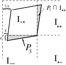
FIG. 4.: The parallelogram $P_{3}={\mathbf{T}}_{{\epsilon},{\delta}}(S_{3})$ and its intersection with the square $I_{++}$.

The pre–image set of the overlap, ${\mathbf{T}}_{{\epsilon},{\delta}}^{-1}\left(OV_{-+,++}\right)$, is displayed in figure 5 where we restrict the parameter range to $-2\,\epsilon<\delta<0$ for simplicity. For calculating pre–images of higher order the so called ”blind area” $B_{-+}$ comes into play, i. e. the set of points in $I_{-+}$ which do not have pre–images with respect to the map ${\mathbf{T}}_{{\epsilon},{\delta}}$. The components of ${\mathbf{T}}_{{\epsilon},{\delta}}^{-1}\left(OV_{-+,++}\right)$ in $S_{1}$ and $S_{2}$ are contained in the subset $T$ of the blind area $B_{-+}$ (cf. figure 5). In first order the width of the set $T$ is given by the expression

$$b_{T}\left(x_{2}\right)=\epsilon+\epsilon\,x_{2}\,,\quad x_{2}\in[0,1]\;.$$ (B3)

FIG. 5.: The pre–image set ${\mathbf{T}}_{{\epsilon},{\delta}}^{-1}\left(OV_{-+,++}\right)$ and its four components in the rectangles $S_{i}$ ($-2\,\epsilon<\delta<0$). Additionally the blind area $B_{-+}$ and its subset $T$ (cf. eq. (B3)) are displayed in gray.

For convenience in calculating pre–images of higher order we first concentrate on the right rectangles $S_{3}$ and $S_{4}$. Defining the generations of order $k$ by

$$G^{(1)} := {\mathbf{T}}^{-1}_{{\epsilon},{\delta}}(OV_{-+,++})\cap(\,S_{3}\cup S_{4}\,)\;,$$ (B4)

$$G^{(k)} := \left\{{\mathbf{x}}\in\left(\,S_{3}\cup S_{4}\,\right)\;|\;{\mathbf{T}}_{{\epsilon},{\delta}}({\mathbf{x}})\in G^{(k-1)}\right\}\;,\quad\;k=2,3,\dots$$ (B5)

figure 6 reveals a beautiful recursive structure of these sets. In order to describe this structure analytically we remark that up to first order it is sufficient to compute pre–images with respect to a simplified map (cf. eq. (A12))

$$\left[\widetilde{{\mathbf{T}}}_{\epsilon,\delta}({\mathbf{x}})\right]_{1} = 2{x}_{1}+\epsilon f_{0}(x_{2})$$ (B6)

$$\left[\widetilde{{\mathbf{T}}}_{\epsilon,\delta}({\mathbf{x}})\right]_{2} = f_{0}({x}_{2})\quad.$$ (B7)

Then the following properties of the generations $G^{(k)}$, which are inherent in figure 6, are easily obtained

• The first generation $G^{(1)}$ consists of two triangles with vertices $(0,0)$, $(0,1/2)$, $(-\epsilon/2,1/2)$ respectively $(0,1)$, $(0,1/2)$, $(-\epsilon/2,1/2)$.

• A generation $G^{(k)}$ encompasses $2^{k}$ triangles each of them having the same area. The area shrinks by a factor 4, if one passes from $G^{(k-1)}$ to $G^{(k)}$.

• Two neighbouring triangles of the same generation share a corner or a side with length of order $\epsilon$.

• The union $\Sigma_{G}^{(k)}:=\cup_{n=1}^{k}\,G^{(n)}$ is a simply connected set.

To determine the boundary of $\Sigma_{G}^{(k)}$ we consider its height function

$$R^{(k)}(x_{2}):=\inf\left\{\,x_{1}\;|\;(x_{1},\,x_{2})\in\Sigma_{{G}}^{(k)}\;\right\}\;.$$ (B8)

Since $R^{(k+1)}$ is mapped on $R^{(k)}$ by the simplified map $\widetilde{{\mathbf{T}}}_{{\epsilon}}$, we get the representation

$$R^{(k)}(x_{2})=-\epsilon\;\sum_{i=1}^{k}\frac{f_{0}^{i}(x_{2})}{2^{i}}\,,\quad\quad x_{2}\in[0,1]\quad.$$ (B9)

For $k$ odd these curves admit $2^{(k-1)/2}$ absolute extrema at

$$x_{min}\in\left\{\frac{1}{2}\,\left(1+\sum_{j=1}^{(k-1)/2}\frac{i_{j}}{4^{j}}\right)\;\bigg{|}\quad i_{j}\in\{-1,+1\},\;j=1,2,\dots(k-1)/2\right\}$$ (B10)

with height

$$R^{(k)}(x_{min})=-\frac{\epsilon}{2}\,\sum_{i=0}^{(k-1)/2}\,\frac{1}{4^{i}}\;.$$ (B11)

In the limit $k\to\infty$ the set $\Sigma_{G}^{\infty}$ has a fractal boundary, since its construction is analogous to the famous Koch’s curve [17]. The thickness of the set $\Sigma_{G}^{\infty}$ follows easily from eq. (B11)

$$h\left(\Sigma_{{G}}^{\infty}\right):={\rm sup}\left\{\,|x_{1}|\;|\;{\mathbf{x}}\in\Sigma_{{G}}^{\infty}\,\right\}=\frac{2\,\epsilon}{3}\;.$$ (B12)

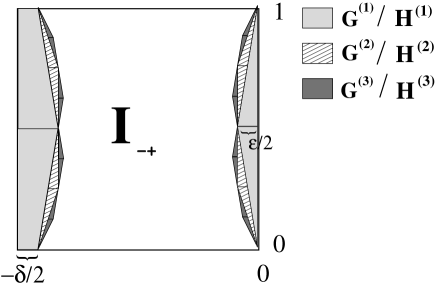
FIG. 6.: The first three generations $G^{(k)}$ and $H^{(k)}$ near the right resp. left edge of $I_{-+}$ .

A generation ${G}^{(k)}$ has not only pre–images ${G}^{(k+1)}$ in the right rectangles $S_{3}$ and $S_{4}$, but there are also pre–images in the left rectangles $S_{1}$ and $S_{2}$ (cf. figure 6)

$$H^{(1)} := {\mathbf{T}}^{-1}_{{\epsilon},{\delta}}(OV_{-+,++})\,\cap\,(\,S_{1}\cup S_{2}\,)\,,$$ (B13)

$$H^{(k)} := \left\{{\mathbf{x}}\in\left(\,S_{1}\cup S_{2}\,\right)\;|\;{\mathbf{T}}_{{\epsilon},{\delta}}({\mathbf{x}})\in G^{(k-1)}\right\}\,,\quad\;k=2,3,\dots\quad.$$ (B14)

To reveal the relation between $G^{(k)}$ and $H^{(k)}$ analytically we just note that for a point ${\mathbf{y}}\in G^{(k-1)}$ eqs. (B5) and (B14) imply that

$\displaystyle{\mathbf{T}}_{{\epsilon},{\delta}}({\mathbf{x}})={\mathbf{T}}_{{\epsilon},{\delta}}({\mathbf{x^{\prime}}})={\mathbf{y}}\in G^{(k-1)}\,,\quad\;{\mathbf{x}}\in G^{(k)},\;{\mathbf{x^{\prime}}}\in H^{(k)}\;.$

Then to first order

$$x_{1}^{\prime}+1=-\delta/2-{x}_{1},\quad x_{2}^{\prime}=x_{2}$$ (B15)

follows. Hence, the set $H^{(k)}$ is obtained from $G^{(k)}$ by a reflection and an additional offset of $-\delta/2$ (cf. figure 6). The same property follows of course for the limits $\Sigma_{H}^{\infty}$ and $\Sigma_{G}^{\infty}$.

If

$$\Sigma_{H}^{\infty}\subset B_{-+}\;,$$ (B16)

holds, no further pre–images of the overlap set $OV_{-+,++}$ appear, and the union $\Sigma_{G}^{\infty}\cup\Sigma_{H}^{\infty}$ encompasses all pre–images. Consequently, the transition $I_{-+}\rightarrow I_{++}$ is not possible, because all pre–images of the overlap set are located near the edge of $I_{-+}$. Therefore, condition (B16) gives the clue for the determination of $\delta_{crit.}(\epsilon)$.

According to eqs. (B15) and (B12) the thickness of $\Sigma_{H}^{\infty}$ reads

$$h\left(\Sigma_{H}^{\infty}\right):={\rm sup}\{\,1+x_{1}\;|\;{\mathbf{x}}\in\Sigma_{H}^{\infty}\,\}=-\frac{\delta}{2}+\frac{2\,\epsilon}{3}\;.$$ (B17)

At the critical value $\delta_{crit.}(\epsilon)$ one peak at the boundary with maximal height collides with the right border of the set $T\subset B_{-+}$ (cf. figure 7). Since the boundary of the blind area has according to eq. (B3) a finite slope, the peak with the smallest $x_{2}$ coordinate crosses the right boundary of $T$ at first. According to eq. (B10) this peak is located at $x_{2}=1/3$. Then eqs. (B17) and (B3) yield

$$\frac{2}{3}\,\epsilon-\frac{\delta_{crit.}(\epsilon)}{2}=h\left(\Sigma_{H}^{\infty}\right)=b_{T}\left(x_{2}=1/3\right)=\frac{4}{3}\epsilon$$ (B18)

and consequently we arrive at

$$\delta_{crit.}(\epsilon)=-\frac{4}{3}\epsilon\;.$$ (B19)

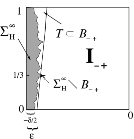
FIG. 7.: Diagrammatic view of the set $\Sigma_{H}^{\infty}$ and the subset $T\subset B_{-+}$ of the blind volume for $\delta<\delta_{crit.}(\epsilon)$.

In order to show that the transition $I_{-+}\rightarrow I_{++}$ is possible for $\delta<\delta_{crit.}(\epsilon)$ the two conditions mentioned at the end of section II have to be checked. Since $\Sigma_{H}^{\infty}\setminus B_{-+}$ is non–empty for $\delta<\delta_{crit.}(\epsilon)$, there exists an open neighbourhood of $(x_{1},x_{2})=(-1,1/3)$ which is contained within the pre–image set ${\mathbf{T}}_{{\epsilon},{\delta}}^{-k_{0}}\left(OV_{-+,++}\right)$ for a particular value $k_{0}$. Next pre–images are located near $(-1/2,1/6)$ and $(-1/2,5/6)$ and hence enter the inner part of the square $I_{-+}$. For higher generations again four pre–images exist. Therefore it is plausible – and more intricate considerations of [12] confirm it – that the set $\cup_{k=0}^{\infty}\,{\mathbf{T}}_{{\epsilon},{\delta}}^{-k}\left(OV_{-+,++}\right)$ has a substantial Lebesgue measure. For the second transition criterion we have to check whether the points that are mapped into the overlap $OV_{-+,++}$ can migrate into the inner part of $I_{++}$ under further iteration. A point ${\mathbf{x}}\in OV_{-+,++}$ has a positive $x_{1}$ coordinate of order ${\cal O}(\epsilon)$. If one considers the evolution of the $x_{1}$ coordinate (cf. eq. (B7)), its value grows for most points ${\mathbf{x}}\in OV_{-+,++}$ under further iteration, until it reaches a value of order one. Therefore, the iterates reach the inner part of $I_{++}$ after a finite number of steps.

In conclusion, the transition $I_{-+}\rightarrow I_{++}$ becomes possible for $\delta<\delta_{crit.}\left(\epsilon\right)$. Computation for other transitions or a CML with $N=3$ follows the same lines. We stress that the main steps consist in the calculation of images and pre–images of overlap sets. The location of the pre–image sets relative to the blind volume determines whether all pre–images of the overlap set are located near the edge of the cube only. Consequently, the existence of the blind volume influences the numerical value of $\delta_{crit.}(\epsilon)$ significantly.

C

In this appendix we would like to show that for $N=2$ the cubes $I_{-+}$ and $I_{+-}$ contain attractors in the strict mathematical sense, if $\delta>-4\,\epsilon/3$. Because of symmetry we can concentrate on the cube $I_{-+}$. In appendix B we have shown that the (dominant) transitions $I_{-+}\rightarrow I_{++}$ and $I_{-+}\rightarrow I_{--}$ are forbidden, as long as $\delta>\delta_{crit.}\approx-4\,\epsilon/3$. What remains to be done is that also the off diagonal transition $I_{-+}\rightarrow I_{+-}$ does not appear.

If $\delta<0$ there exists a non–empty overlap set. Considering the four rectangles in $I_{-+}$ on which the CML ${\mathbf{T}}_{{\epsilon},{\delta}}$ is linear (cf. eq. (A3)), only the image of the rectangle $S_{-2\,2}:=[-1,\,-a]\times[a,\,1]$ intersects the square $I_{+-}$ for $\delta<0$.

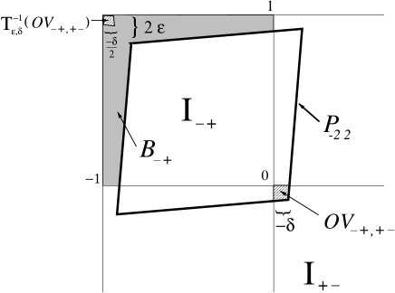
FIG. 8.: The overlap set $OV_{-+,+-}$ and its pre–image ${\mathbf{T}}_{{\epsilon},{\delta}}^{-1}(OV_{-+,+-})$.

Figure 8 displays this situation where the parallelogram $P_{-2\,2}={\mathbf{T}}_{{\epsilon},{\delta}}(S_{-2\,2})$ and the overlap set

$$OV_{-+,+-}=P_{-2\,2}\cap I_{+-}$$ (C1)

are shown. The overlap set has extension $\approx-\delta$ in the directions of both coordinate axes and hence an area $\approx\delta^{2}$. Note that this area is factor of the order ${\cal O}(\epsilon,\,\delta)$ smaller than those of the overlap sets $OV_{-+,++}$ and $OV_{-+,--}$ which belong to perturbatively dominant transitions.

The overlap set (C1) alone does not ensure for a transition $I_{-+}\rightarrow I_{+-}$. In fact we show that phase space trajectories do not reach this set, so that the transition does not appear. Since we are considering a map with a finite coupling $\epsilon>0$, trajectories do not fill the whole phase space $[-1,1]^{2}$ but only the subset ${\mathbf{T}}_{{\epsilon},{\delta}}([-1,1]^{2})\subset[-1,1]^{2}$. In particular points close to the upper left corner of $I_{-+}$ are not visited. This forbidden domain, previously called the blind volume, constitutes the reason why the off diagonal transition does not appear even beyond the perturbation theory.

To put the argument on a formal level we construct the pre–image sets of the overlap set within the square $I_{-+}$. The first generation set, ${\mathbf{T}}_{{\epsilon},{\delta}}^{-1}(OV_{-+,+-})$ is located near the corner $(-1,\,1)$ of $I_{-+}$ and has sides of length $\approx-\delta/2$ (cf. figure 8). As also shown in this figure, the blind area $B_{-+}$ of the square $I_{-+}$ is also located there and contains a square with side length $2\,\epsilon$. Therefore, the pre–image set ${\mathbf{T}}_{{\epsilon},{\delta}}^{-1}(OV_{-+,+-})$ is contained in the blind area, as long as $\delta>-4\,\epsilon$. Hence in this parameter regime the overlap set has no pre–image sets ${\mathbf{T}}_{{\epsilon},{\delta}}^{-k}(OV_{-+,+-})$ with $k\geq 2$, because points belonging to the blind area have no pre–images themselves. In particular, the pre–images of the overlap set do not intersect the inner part of the square $I_{-+}$, so that one criterion for the transition $I_{-+}\rightarrow I_{+-}$ is not obeyed and the transition is impossible for $\delta>-4\,\epsilon$.

Summarising, none of the transitions $I_{-+}\rightarrow I_{\bm{\alpha}}$ with $\bm{\alpha}\in\{--,\;++,\;+-\}$ is possible for $\delta>\delta_{crit.}\approx-4\,\epsilon/3$. Therefore, in this parameter region attractors in the strict sense reside within the squares $I_{-+}$ and $I_{+-}$.

REFERENCES

- [1] J. P. Eckmann and D. Ruelle, Rev. Mod. Phys. 57, 617 (1986).
- [2] K. Kaneko (Ed.), Theory and Applications of Coupled Map Lattices (Wiley, Chichester, 1993).
- [3] J. P. Crutchfield and K. Kaneko, in Directions in Chaos, edited by H. Bai–Lin (World Scientific, Singapore, 1987), Vol. 1.
- [4] C. Robinson, Dynamical systems: Stability, Symbolic Dynamics, and Chaos (CRC Press, Boca Raton, 1995).
- [5] L. A. Bunimovich and Y. G. Sinai, Nonlinearity 1, 491 (1988).
- [6] J. Bricmont and A. Kupiainen, Nonlinearity 8, 379 (1995).
- [7] G. Nicolis and C. Nicolis, Phys. Rev. A 38, 427 (1988).
- [8] T. Bohr, M. H. Jensen, G. Paladin, and A. Vulpiani, Dynamical Systems Approach to Turbulence (Cambridge University Press, Cambridge, 1998).
- [9] H. Sakaguchi, Prog. Theor. Phys. 80, 7 (1988).
- [10] J. Miller and D. A. Huse, Phys. Rev. E 48, 2528 (1993).
- [11] P. Marcq, H. Chaté, and P. Manneville, Phys. Rev. E 55, 2606 (1997).
- [12] F. Schmüser, Ph.D. thesis, Universität Wuppertal, 1999, electronic version available at the web page http://www.bib.uni-wuppertal.de/elpub/ed-liste.html#Physik
- [13] R. J. Glauber, Journ. of Math. Physics 4, 294 (1963).
- [14] K. Kawasaki, Phase Transitions and Critical Phenomena (Academic Press, London, 1972), Vol. 2, p. 443.
- [15] P. C. Hohenberg and B. I. Halperin, Rev. Mod. Phys. 49, 435 (1977).
- [16] V. Privman (Ed.), Nonequilibrium Statistical Mechanics in One Dimension (Cambridge University Press, Cambridge, 1997).
- [17] B. Mandelbrot, The Fractal Geometry of Nature (W. H. Freeman, New York, 1977).