Ordered and self–disordered dynamics of holes and defects in the one–dimensional complex Ginzburg–Landau equation

Abstract

We study the dynamics of holes and defects in the 1D complex Ginzburg–Landau equation in ordered and chaotic cases. Ordered hole–defect dynamics occurs when an unstable hole invades a plane wave state and periodically nucleates defects from which new holes are born. The results of a detailed numerical study of these periodic states are incorporated into a simple analytic description of isolated “edge” holes. Extending this description, we obtain a minimal model for general hole–defect dynamics. We show that interactions between the holes and a self–disordered background are essential for the occurrence of spatiotemporal chaos in hole–defect states.

The formation of local structures and the occurrence of spatiotemporal chaos are the most striking features of pattern forming systems. The complex Ginzburg–Landau equation (CGLE)

$$A_{t}=A+(1+ic_{1})\nabla^{2}A-(1-ic_{3})|A|^{2}A$$ (1)

provides a particularly rich example of these phenomena. The CGLE describes pattern formation near a Hopf bifurcation and has become a paradigmatic model for the study of spatiotemporal chaos [2, 3, 4, 5, 6, 7, 8]. Defects occur when $A$ goes through zero and the complex phase $\psi\!:=\!\arg(A)$ is no longer defined. In two and higher dimensions, such defects can only disappear via collisions with other defects, and act as long–living seeds for local structures like spirals [4] and scroll waves [5] whose instabilities lead to various chaotic states [4, 5]. For the 1D CGLE, however, defects occur only at isolated points in space–time (see Fig. 1) and intricate dynamics of defects and local hole structures occurs, especially in the so–called intermittent and bi–chaotic regimes [6]. The holes are characterized by a local concentration of phase–gradient $q\!:=\partial_{x}\psi$ and a depression of $|A|$ (hence the name “hole”), and dynamically connect the defects (Fig. 1). We divide these holes into two categories: coherent and incoherent structures.

Coherent structures - By this we mean uniformly propagating structures of the form $A(x,t)=e^{-i\omega t}\bar{A}(x-vt)$ [9]. Recently, hole solutions of this form called homoclinic holes were obtained [7]. Asymptotically, homoclinic holes connect identical plane waves where $A\!\sim\!e^{i(q_{ex}x-\omega t)}$. With $c_{1},c_{3}$ and $q_{ex}$ fixed, unique left moving and unique right moving coherent holes are found. Left (right) moving holes with $q_{ex}=Q$ ($q_{ex}=-Q$) are related by the left–right $q\!\leftrightarrow\!-q$ symmetry of the CGLE. Coherent holes have one unstable core mode [7].

Incoherent structures - In full dynamic states of the CGLE, one does not observe the unstable coherent homoclinic holes, unless one fine–tunes the initial conditions (see Fig. 2d). Instead evolving incoherent holes that can

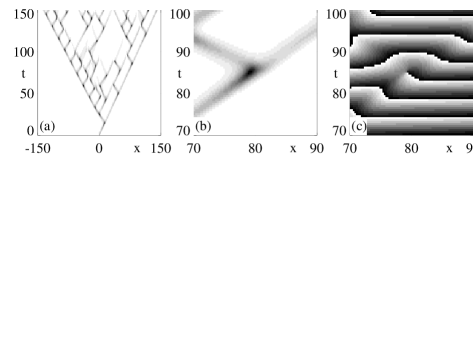
FIG. 1.: (a) A space–time grey–scale plot of $|A|$ (dark: $A\!\approx\!0$), showing the propagation of incoherent holes into a plane wave state. The dark dots correspond to defects. Note the roughly constant velocities at which the holes propagate. Parameter values are $c_{1}\!=\!0.6,c_{3}\!=\!1.4$ , with an initial condition given by Eq. (2), with $\gamma\!=\!1,q_{ex}\!=\!-0.03$. This non–zero $q_{ex}$ breaks the left–right symmetry and results in the differing periods of the left and right moving edge holes. (b–c) Close–up of $|A|$ (b) and the complex phase $\psi$ (c).

grow out to defects occur (Fig. 1 and 2b).

In this Letter we study the hole $\!\rightarrow\!$ defect and defect $\!\rightarrow\!$ holes dynamical processes of the 1D CGLE [10]. We present a minimal model for hole–defect dynamics that describes the full “interior” spatiotemporal chaotic states of Fig. 1a, where holes propagate into a self–disordered background. Similar “self–replicating” patterns are observed in many other situations, e.g., reaction–diffusion models [11], film–drag [12], eutectic growth [13], forced CGLE [14] and space–time intermittency models [15].

Hole $\!\rightarrow\!$ defect - Let us consider the short–time evolution of an isolated hole propagating into a plane wave state. Holes can be seeded from initial conditions like:

$$A=\exp(i[q_{ex}x+(\pi/2)\tanh(\gamma x)])~{}.$$ (2)

The precise form of the initial condition is not important here as long as we have a one–parameter family of localized phase–gradient peaks. This is because the left moving and right moving coherent holes for fixed $c_{1},c_{3}$ and $q_{ex}$ are each unique and have one unstable mode only. As $\gamma$ is varied three possibilities can arise for the time

FIG. 2.: (a) Schematic representation of the phase space of the CGLE around the homoclinic hole solution, showing: the 1D unstable manifold $W^{\rm u}$; the high dimensional neutral/stable manifold $W^{\rm ns}$ that separates decaying from defect forming states; the manifold $\Gamma$ representing the family of peaked initial conditions of the form (2). (b–d) Four snapshots $(\Delta t\!=\!10)$ of the $q$-profile of a right moving hole where $q_{ex}\!=\!0$, $c_{1}\!=\!0.6$, and $c_{3}\!=\!1.4$. The peaked initial condition is given by Eq. (2): (b) A hole evolving to a defect $(\gamma=0.568)$, (c) a decaying hole $(\gamma=0.5)$, and (d) a hole evolving close to a coherent structure $(\gamma=0.5545)$.

evolution of the initial peak: evolution towards a defect (as in Fig. 1a), decay, or evolution arbitrary close to a coherent homoclinic hole (see Fig. 2).

The hole propagation velocities are much larger than the typical group velocities in the plane wave states: the holes are thus only sensitive to the leading wave. Their internal, slow dynamics determines their trailing wave. A (nearly) coherent hole will, due to phase conservation, have a trailing wave (nearly) identical to the leading wave (Fig. 2); hence the relevance of the homoclinic holes.

Defect $\!\rightarrow\!$ holes - What dynamics occurs after a defect has been formed? A study of the spatial defect profiles reveals that they consist of a negative and positive phase–gradient peak in close proximity (the early stage of the formation of these two peaks can be seen in Fig. 2b; see also Fig. 4d of [7]). The negative (positive) phase gradient peak generates a left (right) moving hole. The lifetimes of these holes depend on their parent defect profile (analogous to what we described in Fig. 2) and also on $c_{1},c_{3}$ and $q_{ex}$. Hence the defects act as seeds for the generation of daughter holes (see also Fig. 1).

Periodic hole-defect states - When an incoherent hole invades a plane wave state and generates defects, stable periodic hole $\!\rightarrow\!$ defect $\!\rightarrow\!$ hole behavior can set in at the edges of the resulting pattern [16] (Fig 1a). The asymptotic period $\tau$ of this process depends on $c_{1},c_{3}$, the propagation direction and the wavenumber $q_{ex}$ of the initial condition only; we focus here on right moving holes. The period $\tau$ diverges at a well–defined value of $q_{ex}\!=\!q_{coh}$ (Fig. 3a). This can be understood in the phase space picture presented in Fig. 2. Suppose we fix $c_{1}$ and $c_{3}$. The edge defects that are generated periodically yield

FIG. 3.: (a) Log–linear plot of the period $\tau$ as a function of $q_{ex}-q_{coh}$. (b) $100/q_{m}$ as a function of the time $\Delta t$ before the formation of a defect; (c) $\dot{q}_{m}$ as a function of $q_{m}$.

constant initial conditions for their daughter edge holes, similar to fixing $\gamma$ in Eq. (2). The period $\tau$ will depend on the location of the defect profile with respect to the stable manifold of the coherent hole. When $q_{ex}$ is varied, both this manifold and the defect profile may change, and for a certain value of $q_{ex}$ which we call $q_{coh}$, the defect generates an initial condition precisely on the stable manifold of the coherent hole. The lifetime of the resulting daughter hole then diverges (see Fig. 2d).

To substantiate this intuitive picture, we have performed numerics on the dynamics of “edge–holes” invading a plane wave state where $A\sim e^{i(q_{ex}x-\omega t)}$. We have performed runs for many different parameters, but will only discuss a representative subset here. Our results indicate that the $\tau$ divergence is of the form

$$\tau\sim-s\ln(q_{ex}-q_{coh})+\tau_{0}~{}.$$ (3)

This equation, and in particular the value of $s$ can be understood by considering the flow near the saddle point shown in Fig 2a. Just after the hole has been formed, it first evolves rapidly along the stable manifold. Secondly it evolves slowly along the unstable manifold before being shot away towards the next defect. For values of $q_{ex}$ close to $q_{coh}$, the holes approach the coherent structure fixed point very closely, and $\tau$ will be dominated by a regime of exponential growth close to this fixed point. Small changes in $q_{ex}$ will have a negligible effect on the duration of the first phase ($\tau_{0}$), but the duration of the second phase will diverge logarithmically as $~{}-(1/\lambda)\ln(q_{ex}-q_{coh})$. Here $\lambda$, which depends on $c_{1}$ and $c_{3}$, denotes the unstable eigenvalue of the coherent structures at $q_{ex}\!=\!q_{coh}$. In Table 1 we list some numerically determined values for $q_{coh}$, $1/\lambda$, and $s$. We obtained $s$ and $q_{coh}$ from a fit of $\tau$ to Eq. (3), whereas $\lambda$ is obtained from a shooting algorithm, see Ref. [7]. The agreement between $s$ and $1/\lambda$ is quite satisfactory.

We will now construct a phenomenological model for isolated incoherent holes. (i) We will ignore their early time attraction to the unstable manifold, and think of their location on $W^{\rm U}$ as an internal degree of freedom, parameterized by the phase–gradient extremum $q_{m}$. (ii) Clearly the model should have an unstable fixed point for values of $q_{m}$ corresponding to coherent holes. We have found that, in good approximation, coherent holes have

$c1$	$c3$	$q_{coh}$	1/$\lambda$	$s$
0.6	1.4	-0.0362	8.42	8.4
0.8	1.4	-0.0727	9.91	9.5
0.6	1.2	0.0538	12.72	12.7
1.0	1.2	-0.0200	17.71	18.7

Table 1. Comparison of $1/\lambda$ with $s$ (see text for details).

$q_{m}\!=\!q_{n}\!+\!gq_{ex}$ where $q_{n}$ denotes the value of $q_{m}$ for a coherent hole in a $q_{ex}\!=\!0$ state, and $g$ is a negative phenomenological constant. (iii) When approaching a defect, $q_{m}$ diverges as $(\Delta t)^{-1}$ [17]; we have confirmed this by accurate numerics (Fig. 3b). An appropriate equation incorporating these three features is

$$\dot{q}_{m}=\lambda(q_{m}-(q_{n}+gq_{ex}))+\mu(q_{m}-(q_{n}+gq_{ex}))^{2}~{},$$ (4)

where $g$ and $\mu$ are phenomenological constants. The first term on the RHS of (4) results from the linearization near the coherent fixed point. Nonlinear terms of higher than quadratic order on the RHS of Eq. (4) are ruled out by the $(\Delta t)^{-1}$ divergence of $q_{m}$. Our numerical data for $\dot{q}_{m}$ versus $q_{m}$ indeed shows quadratic behavior for large enough values of $q_{m}$ (Fig. 3c). For smaller values of $q_{m}$, the curves are quite intricate; this corresponds to the rapid early time evolution along the stable manifold not included in model (4). From Eq. (4), it is straightforward to show that the hole lifetime $\tau$ (the time taken for $q_{m}$ to diverge) displays the required logarithmic divergence as $q_{ex}$ is tuned towards a critical value $q_{coh}$.

Disordered dynamics - If the patches away from the holes/defects were simply plane waves with fixed wavenumber, then one would expect, following the arguments given above, quite regular dynamics. The coupling between holes and the background induced by phase conservation becomes the key ingredient to understand disorder in hole–defect dynamics such as shown in Fig 1a. Let us introduce a variable $\phi:=\int dxq$ that measures the phasedifference across a certain interval.

Consider again an edge hole evolving towards a defect. While the peak of the $q$-profile grows, the hole creates a dip in its wake (see Fig. 2b) in order to locally conserve $\phi$. Clearly the trailing edge of this incoherent hole is not a perfect plane wave. In the interior of states such as shown in Fig. 1a, unstable holes move back and forth through a background of disordered $q_{ex}$ and amplify this disorder. Nevertheless, as we pointed out earlier, the disordering dynamics is sufficiently slow such that the holes remain approximately homoclinic for much of their lives. Although the typical range of values for the disordered $q_{ex}$ is small, the hole lifetimes depend on it sensitively. Hence the variation in $q_{ex}$ and $\phi$ is sufficient to explain the varying lifetimes found in the interior states such as that shown in Fig 1a. Thus the essence of the spatiotemporal chaotic states here lies in the propagation of unstable local structures in a self–disordered background.

Minimal model - To illustrate our picture of self–disordered dynamics, we will now combine the various hole–defect properties with the left–right symmetry and local phase conservation of the CGLE to form a minimal model of hole–defect dynamics. From our previous analysis, we see that the following hole–defect properties should be incorporated: (i) Incoherent holes propagate either left or right with essentially constant velocity (see Fig. 1a). (ii) For fixed $c_{1},c_{3}$, their lifetime depends on the profile of their parent defect, the direction of propagation, and on the wavenumber of the state into which they propagate. (iii) Eq. (4) captures essentially all aspects of the evolution of their internal degree of freedom. When $q_{m}$ diverges, a defect occurs.

In our model we will assume that all the defects have the same profile and so act as unique initial conditions for their daughter incoherent holes. While in principle a defect profile could depend on the entire history of the hole which preceded it, for simplicity we have chosen to neglect this. We have observed that for some regions of the $c_{1},c_{3}$ parameter space, the defect profiles from the interior spatiotemporal chaotic patterns show a surprising lack of scatter [10]. Therefore we believe that treating the defect profiles as constant, and only including the effect of the background in the hole dynamics incorporates the essence of the coupling to a disordered background.

We discretize both space and time by coarse-graining, and take a “staggered” type of update rule which is completely specified by the dynamics of a $2\times 2$ cell (see Fig. 4a). We put a single variable $\phi_{i}$ on each site, corresponding to the phase difference across a cell divided by $2\pi$. Local phase conservation is implemented by $\phi^{\prime}_{l}\!+\!\phi^{\prime}_{r}\!=\!\phi_{l}\!+\!\phi_{r}$, where the primed (unprimed) variables refer to values after (before) an update.

Holes are represented by active sites where $|\phi|>\phi_{t}$; here $\phi$ plays the role of the internal degree of freedom. Inactive sites are those with $|\phi|<\phi_{t}$, and they represent the background. The value of the cutoff $\phi_{t}$ is not very important as long as it is much smaller than typical values of $\phi$ for coherent holes. Here $\phi_{t}$ is fixed at $0.15$. Without loss of generality we force holes with positive (negative) $\phi$ to propagate only from $\phi_{l}$ ($\phi_{r}$) to $\phi^{\prime}_{r}$ ($\phi^{\prime}_{l}$).

Depending on the two incoming states, we have the following three possibilities:

One site active: Without loss of generality we assume that we have a right moving hole. We implement evolution similar to Eq. (4), but neglect the quadratic term of Eq. (4); even though $q_{m}$ diverges, the local phasedifference $\phi_{m}$ does not diverge near a defect. Hence the finite time divergence of the local phase gradient $q$ that signals a defect can be replaced by a cutoff $\phi_{d}$ for $\phi$. Therefore, when $\phi_{l}\!<\!\phi_{d}$, the internal hole coordinate $\phi$ is taken to evolve via $\phi^{\prime}_{r}\!=\phi_{l}+\!\lambda(\phi_{l}-\phi_{n}-g\phi_{r})$. Here $\lambda$ sets the time scales and can be taken small (fixed at $0.1$). This evolution equation, combined with the local phase conservation, means that an incoherent hole propagating

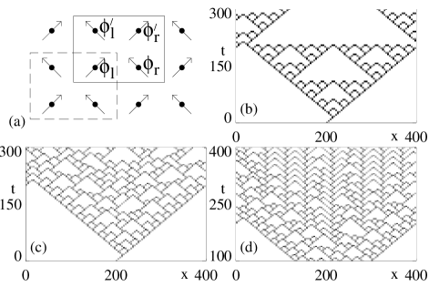
FIG. 4.: (a) Grid model geometry showing the sites (dots) and hole propagation direction (arrows). The update rule is defined within a $2\times 2$ cell. (b–d) Dynamical states in the grid model, for $\phi_{n}\!=\!0.6$ and $\phi_{ad}\!=\!0.75$. Initial condition: center site has $\phi\!=\!0.7$, everywhere else $\phi\!=\!0$ (hence the symmetric patterns). (b) $g\!=\!0$ and $\phi_{d}\!=\!1$. (c) Disordered dynamics for nonzero coupling ($g\!=\!-3,\phi_{d}\!=\!1$). (d) Zigzag structures occur for $g\!=\!-3,\phi_{d}\!=\!0.98$.

into a perfect laminar state will leave a disordered state in its wake. When $\phi_{l}>\phi_{d}$, a defect occurs and two new holes are generated: $\phi^{\prime}_{r}=\phi_{ad}$, and $\phi^{\prime}_{l}=\phi_{d}-1-\phi_{ad}$. The factor $-1$ reflects the change in winding number at a defect.

Both sites inactive: Away from the holes/defects, the relevant dynamics is phase diffusion. This is implemented via: $\phi^{\prime}_{r}\!=\!D\phi_{l}\!+\!(1\!-\!D)\phi_{r}$. The value of $D$ is fixed at $0.05$ and is not very important.

Both sites active: This corresponds to the collision of two oppositely moving holes. Typically this leads to the annihilation of both holes (see Fig. 1a), which we implement here via phase conservation: $\phi^{\prime}_{r}\!=\!\phi^{\prime}_{l}\!=\!(\phi_{l}\!+\!\phi_{r})/2$.

The coupling of the holes to their background, $g$, should be taken negative (although its precise value is unimportant). For $g\!=\!0$ the lifetime $\tau$ becomes a constant, independent of the $\phi$ of the state into which the holes propagate, and moreover, the dynamical states are regular Sierpinsky gaskets (Fig. 4b). Nevertheless, starting from a $\phi\!=\!0$ state, the local phase conservation of the hole dynamics leads to a background state with a disordered $\phi$ profile. For $g\!<\!0$ the coupling to this background leads to disorder as shown in Fig. 4c,d. This illustrates the crucial importance of the coupling between the holes and the self–disordered background.

The essential parameters determining the qualitative nature of the overall state are $\phi_{n}$, $\phi_{d}$ and $\phi_{ad}$. These parameters determine the amount of phase winding in the core of the $q_{ex}\!=\!0$ coherent holes ($\phi_{n}$) and in the new holes generated by defects ($\phi_{ad},\phi_{d}-1-\phi_{ad}$). When varying the CGLE coefficients $c_{1},c_{3}$, these parameters change too; for example, $\phi_{n}$ typically decreases when $c_{1}$ or $c_{3}$ are increased. As a result, for large values of $c_{1}$ and $c_{3}$, $|\phi^{\prime}_{l}|$ and $\phi^{\prime}_{r}$ are typically larger than $\phi_{n}$ so that most “daughter holes” will grow out to form defects and hole-defect chaos spreads (Fig. 4c,d). For sufficiently small values of $c_{1}$ and $c_{3}$, on the other hand, $\phi_{n}$ is large and both daughter holes will decay. For intermediate values of $c_{1}$ and $c_{3}$ it may occur that $|\phi^{\prime}_{l}|$ is significantly larger than $\phi^{\prime}_{r}$, leading to zigzag states [6] (Fig. 4d).

In conclusion, we have studied in detail the dynamics of local structures in the 1D CGLE. We have obtained a quantitative understanding of the edge holes, unraveled the interplay between defects and holes, and put forward a simple model for some of the spatiotemporal chaotic states occurring in the CGLE.

M.v.H. acknowledges support from the EU under contract ERBFMBICT 972554. M.H. acknowledges support from the Niels Bohr Institute, the NSF through the Division of Materials Research, and NSERC of Canada.

REFERENCES

- [1]
- [2] M. C. Cross and P. C. Hohenberg, Rev. Mod. Phys. 65, 851 (1993).
- [3] B. I. Shraiman et al., Physica D 57, 241 (1992).
- [4] I. S. Aranson, L. Aranson, L. Kramer and A. Weber, Phys. Rev. A 46, R2992 (1992); G. Huber, P. Alstrøm and T. Bohr, Phys. Rev. Lett. 69, 2380 (1992).
- [5] I. S. Aranson, A. R. Bishop and L. Kramer, Phys. Rev. E 57, 5276 (1998); G. Rousseau, H. Chaté and R. Kapral, Phys. Rev. Lett 80, 5671 (1998); K. Nam, E. Ott, P. N. Guzdar and M. Gabbay, Phys. Rev. E 58, 2580 (1998).
- [6] H. Chaté, Nonlinearity 7, 185 (1994).
- [7] M. van Hecke, Phys. Rev. Lett. 80, 1896 (1998).
- [8] L. Brusch, M. G. Zimmermann, M. van Hecke, M. Bär and A. Torcini, Phys. Rev. Lett. 85, 86 (2000).
- [9] W. van Saarloos and P. C. Hohenberg, Physica D 56, 303 (1992); 69, 209 (1993) [Errata].
- [10] A more detailed study is in preparation.
- [11] W. N. Reynolds et al., Phys. Rev. Lett. 72, 2797 (1994); M. Zimmermann et al., Physica D 110, 92 (1997); A. Doelman et al., Nonlinearity 10, 523 (1997); Y. Hayase and T. Ohta, Phys. Rev. Lett. 81, 1726 (1998); Y. Nishiura and D. Ueyama, Physica D 130, 73 (1999).
- [12] D. P. Vallette, G. Jacobs and J. P. Gollub, Phys. Rev. E 55, 4274 (1997).
- [13] S. Akamatsu and G. Faivre, Phys. Rev. E, 58, 3302 (1998).
- [14] H. Chaté, A. Pikovsky and O. Rudzick, Physica D 131, 17 (1999).
- [15] H. Chaté, in Spontaneous Formation of Space–Time Structures and Criticality, eds. T. Riste and D. Sherrington, (Kluwer) 273 (1991).
- [16] The full state that develops in the wake of the incoherent holes is chaotic, i.e. one has exponential sensitivity. For the edge holes, however, local perturbations of the initial condition lead only to a space–time shift, and the asymptotic period is independent of such perturbations.
- [17] To see this note that is a smooth function of and , and express as a function of the real and imaginary parts of : . As a function of time, and are both moving linearly through zero at the defect, and hence we find a divergence of .