submitted to Phys. Rev. B.
Ab-initio study of the anomalies in the
He atom scattering spectra of H/Mo (110) and H/W (110)

Abstract

Helium atom scattering (HAS) studies of the H-covered Mo (110) and W (110) surfaces reveal a twofold anomaly in the respective dispersion curves. In order to explain this unusual behavior we performed density functional theory calculations of the atomic and electronic structure, the vibrational properties, and the spectrum of electron-hole excitations of those surfaces. Our work provides evidence for hydrogen adsorption induced Fermi surface nesting. The respective nesting vectors are in excellent agreement with the HAS data and recent angle resolved photoemission experiments of the H-covered alloy system Mo_0.95Re_0.05 (110). Also, we investigated the electron-phonon coupling and discovered that the Rayleigh phonon frequency is lowered for those critical wave vectors. Moreover, the smaller indentation in the HAS spectra can be clearly identified as a Kohn anomaly. Based on our results for the susceptibility and the recently improved understanding of the He scattering mechanism we argue that the larger anomalous dip is due to a direct interaction of the He atoms with electron-hole excitations at the Fermi level.

I Introduction

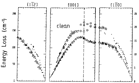
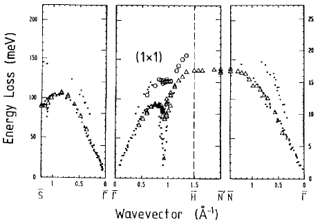
FIG. 1.: HREELS spectra of the clean W(110) surface (upper panel) and its H-covered $(1\times 1)$ phase (lower panel) from Ref. [1]: Shown are the dispersion of the Rayleigh wave (triangles) and the longitudinally polarized surface phonons of the first (circles) and second (squares) layer. The dots represent the results of Hulpke and Lüdecke’s HAS measurements [2, 3].

The interest in the (110) surfaces of Mo and W has been fostered in recent years by the discovery of deep and extremely sharp indentations in the energy loss spectra of He atom scattering at H/Mo (110) and H/W (110) [2, 3]. As depicted in Fig. 1 those anomalies are seen at an incommensurate wavevector, $\overline{Q}^{\rm c,1}_{\rm exp}$, along the $[001]$ direction (${\overline{\Gamma H}}$) and additionally at the commensurate wavevector $\overline{Q}^{\rm c,2}_{\rm exp}=\overline{S}$ at the boundary of the surface Brillouin zone (SBZ). At those points two simultaneous anomalies develop out of the ordinary Rayleigh mode. One, $\omega_{1}$, is extremely deep, and is only seen by helium atom scattering (HAS) [2, 4, 5, 6, 3]. The other, $\omega_{2}$, is instead modest, and is observed by both HAS and high resolution electron energy loss spectroscopy (HREELS) [1, 7, 8]. Since the $[001]$ components of both critical wavevectors $\overline{Q}^{\rm c,1}$ and $\overline{Q}^{\rm c,2}$ are approximately the same it was suggested that the anomaly runs parallel to $\overline{\Gamma N}$ through the SBZ as illustrated in Fig. 2.

FIG. 2.: Position of the HAS anomalies for the H/W(110) adsorbat system within the SBZ. The dotted line indicates the form of the anomaly apart from the symmetry directions $\overline{\Gamma H}$ and $\overline{\Gamma S}$ as suggested by Hulpke and Lüdecke [4].

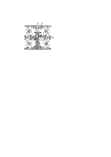
FIG. 3.: ARP-measured Fermi surface of the H-covered W (110) surface [9]. The shaded areas are the (110) projection of the bulk Fermi surface. Surface states at the Fermi level are marked by dots and repeated in the other equivalent sections by crosses. The arrows represent the HAS critical wavevectors $\overline{Q}^{\rm c,1}_{\rm exp}$ and $\overline{Q}^{\rm c,2}_{\rm exp}$.

Various models have been brought forward in order to account for the unusual vibrational properties of H-covered Mo(110) and W(110): For instance, a pronounced but less sharp softening of surface phonons is also seen on the (001) surfaces of W [10] and Mo [11]. There, the effect is caused by marked nesting properties of the Fermi surface [12, 13, 14, 15]. However, angular resolved photoemission (ARP) experiments of H/W (110) and H/Mo (110) gave no evidence for nesting vectors comparable to the HAS determined critical wave vectors [9, 16, 17] (see Fig. 3). Thus, for the phonon anomalies of those two systems there seems to be no connection between the electronic structure and the vibrational properties. Moreover, even if such a relation existed it would be unclear whether the phenomena has to be interpreted as a Kohn anomaly or as the phason and amplitudon modes associated with the occurance of a charge-density wave. In fact, the experimental finding of two modes at $\overline{S}$ as well as some theoretical arguments rule out the phason-amplitudon idea [18]. Furthermore, any model which links the phonon anomalies to the motion of the hydrogen atoms [7] has to be ruled out because the HAS spectra remain practically unchanged when deuterium is adsorbed instead of hydrogen [2, 3].

Still unexplained, but probably not directly correlated to the anomalies, is the peculiar behavior of hydrogen vibrations observed in HREELS experiments by Balden et al. [7, 8]. At a H-coverage of one mono-layer the adsorbate modes parallel to the surface form a continuum interpreted a liquid-like phase of the adsorbate.

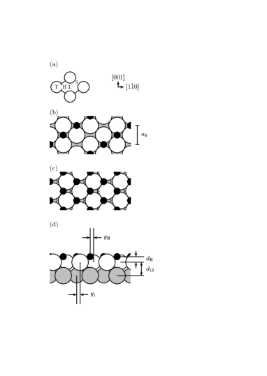
FIG. 4.: (a) Adsorbate positions within the $(1\times 1)$ unit cell of the W (110) and Mo (110) surfaces: Shown are the long-bridge (L), short-bridge (S), hollow (H), and on-top (T) site. (b-c) Structure of the H-covered W (110) surface as suggested by Chung et al. [19]: (b) low H-coverage $\Theta<0.5$ ML; (c) top-layer-shift reconstruction for a H-coverage $\Theta>0.5$ ML. The white (shaded) circles represent the W atoms in the surface (subsurface) layer. The hydrogen positions are indicated by full dots. (d) Illustration of the structure parameters used in Table II. The in-plane lattice constant is denoted by $a_{0}$.

An additional puzzle to the already confusing picture is added by the observation of a symmetry loss in the low-energy electron diffraction (LEED) pattern of W (110) upon H-adsorption. The phenomena was believed being caused by a H-induced displacement of the top layer W atoms along the $[\overline{1}10]$ direction [19] (see Figs. 4b and c). For H/Mo (110) similar studies do not provide any evidence for a top-layer-shift reconstruction [20].

The goal of our work is to give a comprehensive explanation for the observed anomalous behavior and clarify the confusing picture drawn by the different experimental findings. We show that the anomalous behavior observed in the He and electron loss experiments is indeed governed by H-induced nesting features in the Fermi surface.

The remainder of the paper is organized as follows. First, Section II gives a brief introduction into the ab initio method used. The results of our work are presented in Section III: In Subsection III A we study the atomic geometry of the clean and H-covered Mo(110) and W(110) surfaces. In particular, we check whether the hydrogen adsorption induces a top-layer-shift reconstruction. Following in Subsection III B, we focus on the electronic structure of those surface systems. In this context, we are particularily interested in how the Fermi surface changes upon H-adsorption: Is there evidence for Fermi-surface nesting? If yes, how does it connect to the ARP measurements of the Fermi surfaces and the critical wavevectors detected by HAS and HREELS? Along the same line within the model of a Kohn anomaly, Subsection III C digs into the coupling between electronic surface states and surface phonons. There, we discuss the mechanism which causes the small anomaly $\omega_{1}$. In Subsection III D we examine the He scattering mechanism, study the spectrum of electron-hole excitations, and explain the physical nature of the huge anomalous branch $\omega_{2}$. Finally, the major aspects of our work are summarized in Section IV. The Appendix presents several detailed test calculations giving an insight into the properties and the accuracy of our method.

II Method

All our calculations employ the density-functional theory (DFT). They are performed within the framework of the local-density approximation (LDA) for the exchange-correlation energy functional [21, 22]. For the self-consistent solution of the Kohn-Sham (KS) equations we employ a full-potential linearized augmented plane-wave (FP-LAPW) code [23, 24, 25] which we enhanced by the direct calculation of atomic forces [26, 27]. Combined with damped Newton dynamics [28] this enables an efficient determination of fully relaxed atomic geometries. Also, it allows the fast evaluation of phonon frequencies within a frozen-phonon approach.

A LAPW Formalism

There exists a variety of different LAPW programs [24, 29, 30, 31, 32, 33, 34, 35, 36, 37, 38]. We therefore briefly specify the main features of our code. This is also in order to clarify the meaning of the LAPW parameters which determine the numerical accuracy of the calculations.

In the augmented plane-wave method space is divided into the interstitial region (IR) and non-overlapping muffin-tin (MT) spheres centered at the atomic sites [39, 40, 41]. This division accounts for the atomic-like character of the wavefunctions, the potential, and the electron density close to the nuclei and that the behavior of these quantities is smoother in between the atoms. The basis functions $\phi_{\bf K}({\bf r})$ which we employ in our code for the expansion of the electron wavefunctions of the KS equation

$$\psi_{{\bf k},i}({\bf r})=\sum_{|{\bf K}|\leq K^{\rm wf}}C_{i}({\bf K})\phi_{{\bf K}}({\bf r})$$ (1)

are defined as

$$\phi_{\bf K}({\bf r})=\left\{\begin{array}[]{ll}\Omega^{-1/2}\exp(i{\bf K}{\bf r}),&{\bf r}\in{\rm IR}\\ \\ {\displaystyle\sum_{\stackrel{{\scriptstyle\scriptstyle lm}}{{l\leq l^{\rm wf}}}}[a_{lm}^{I}({\bf K})u_{l}^{I}(\epsilon_{l}^{I},r_{I})+b_{lm}^{I}({\bf K})\dot{u}_{l}^{I}(\epsilon_{l}^{I},r_{I})]Y_{lm}(\hat{r}_{I})},&r_{I}\leq s_{I}\quad.\end{array}\right.$$ (2)

Here, $\bf K=\bf k+\bf G$ denotes the sum of a reciprocal lattice vector $\bf G$ and a vector $\bf k$ within the first Brillouin zone. The wavefunction cutoff $K^{\rm wf}$ limits the number of those $\bf K$ vectors and thus the size of the basis set. The other symbols in eq. (2) have the following meaning: $\Omega$ is the unit cell volume, $s_{I}$ specifies the MT radius, and ${\bf r}_{I}={\bf r}-{\bf R}_{I}$ represents a vector within the MT sphere of the $I$-th atom. Note that $Y_{lm}(\hat{r})$ is a complex spherical harmonic with $Y_{l-m}(\hat{r})=(-1)^{m}Y^{*}_{lm}(\hat{r})$. The radial functions $u_{l}(\epsilon_{l},r)$ and $\dot{u}_{l}(\epsilon_{l},r)$ are solutions of the equations

$$H^{\rm sph}\,u_{l}(\epsilon_{l},r)Y_{lm}(\hat{r}) = \epsilon_{l}\,u_{l}(\epsilon_{l},r)Y_{lm}(\hat{r})$$ (3)

$$H^{\rm sph}\,\dot{u}_{l}(\epsilon_{l},r)Y_{lm}(\hat{r}) = [\epsilon_{l}\dot{u}_{l}(\epsilon_{l},r)+u_{l}(\epsilon_{l},r)]Y_{lm}(\hat{r})$$ (4)

which are regular at the origin. Here, the KS operator $H^{\rm sph}$ contains only the spherical average of the effective potential within the respective MT. The expansion energies $\epsilon_{l}$ are chosen somewhere within the respective energy bands with $l$-character, whereas the coefficients $a^{I}_{lm}({\bf K})$ and $b^{I}_{lm}({\bf K})$ are fixed by requiring that value and slope of the basis functions are continuous at the surface of the $I$-th MT sphere. Obviously, this can only be fulfilled for $l\leq l^{\rm wf}$, but as $l^{\rm wf}$ is typically high (e.g. $l^{\rm wf}\geq 8$) this does not represent a problem.

The representation of the potentials and densities resembles the one employed for the wavefunctions, i.e.,

$$V({\bf r})=\left\{\begin{array}[]{ll}\displaystyle\sum_{|{\bf G}|\leq G^{\rm pot}}V_{\bf G}\exp(i{\bf G}{\bf r}),&{\bf r}\in{\rm IR}\\ \\ \displaystyle\hskip 9.95845pt\sum_{\stackrel{{\scriptstyle\scriptstyle lm}}{{l\leq l^{\rm pot}}}}V_{lm,I}(r_{I})Y_{lm}(\hat{r}_{I}),&r_{I}\leq s_{I}\quad.\end{array}\right.$$ (5)

Thus, no shape approximation is introduced. The quality of this full-potential description is controlled by the cutoff parameter $G^{\rm pot}$ for the reciprocal lattice vectors $\bf G$ and the maximum angular momentum $l^{\rm pot}$ of the $(l,m)$-representation inside the MTs.

B Slab Systems and Parametrization

The substrate surfaces are modeled by five-, seven-, and nine-layer slabs repeated periodically and separated by a vacuum region whose thickness is equivalent to four substrate layers. The MT radii for the W and Mo atoms are chosen to be $s_{\rm Mo}=s_{\rm W}=1.27\,$Å. Note that the experimental interatomic distances of bulk Mo and W are 2.73 Åand 2.74 Å, respectively. For hydrogen the MT radius is set to $s_{\rm H}=0.48\,$Å.

In the case of the W surfaces the valence and semi-core electrons are treated scalar-relativistically while the core electrons are handled fully relativistically. For Mo all calculations are done non-relativistically. In both metals we introduce a second energy window for the treatment of the semi-core electrons (4$s$ and 4$p$ for Mo, 5$s$ and 5$p$ for W). The in-plane lattice constants (compare Fig. 4) $a_{\rm W}^{\rm theo}=3.14\,$Å and $a_{\rm Mo}^{\rm theo}=3.13\,$Å are calculated to be without including zero-point vibrations. They are in good agreement with the respective measured bulk lattice parameters at room temperature and other theoretical results (see Appendix 1).

For the potential the $(l,m)$ representation within each MT sphere is taken up to $l^{\rm pot}=4$ while the kinetic-energy cutoff for the interstitial region is set to $\frac{\hbar^{2}}{2m}(G^{\rm wf})^{2}=100$ Ry. Generally, we choose the plane-wave cutoff for the wavefunctions to be $\frac{\hbar^{2}}{2m}(K^{\rm wf})^{2}=12\,$Ry; only for the frozen-phonon calculations we use a slightly smaller cutoff of $\frac{\hbar^{2}}{2m}(K^{\rm wf})^{2}=10\,$Ry which is indeed sufficient. The $(l,m)$ representation of the wavefunctions within the MTs is taken up to $l^{\rm wf}=8$. Also, we employ Fermi smearing with a broadening of $k_{\rm B}T_{\rm el}=68$ meV in order to stabilize the self-consistency and the ${\bf k_{\|}}$-summation. All energies given below are however extrapolations to zero temperature $T_{\rm el}$ [42, 43]. We performed systematic tests comparing the LDA and the generalized gradient approximation [44, 45] exchange-correlation functionals. For the quantities reported in this paper (total energy differences of different adsorption sites, bond lengths, etc.) both treatments give practically the same results. All $\bf k$ sets used were determined by using the special $\bf k$ point scheme of Monkhorst and Pack [46]. Also, we checked the ${\bf k_{\|}}$-point convergence: In the case of atomic and electronic structure calculations a two-dimensional uniform mesh of 64 ${\bf k_{\|}}$-points within the $(1\times 1)$ SBZ gives stable results. For the evaluation of frozen-phonon energies a set of 56 ${\bf k_{\|}}$-points is employed within the SBZ of the enlarged $(1\times 2)$ and $(2\times 1)$ surface cells (see subsection 3 b). In Table I we summarize the main features of our LAPW parameter setting. For more details the reader is referred to the discussion in the Appendix.

TABLE I.: LAPW parameter setting used in Section III for the bulk studies, the calculation of the atomic and electronic surface strucutures, and the evaluation of frozen-phonons.

LAPW	bulk	surface
parameter		structure	phonons
$l^{\rm pot}$	4	4	3
$\frac{\hbar^{2}}{2m}\frac{\hbar^{2}}{2m}(G^{\rm pot})^{2}$ [Ry]	64	100	100
$l^{\rm wf}$	8	8	8
$\frac{\hbar^{2}}{2m}(K^{\rm wf})^{2}$ [Ry]	12	12	10
Fermi smearing [meV]	68	68	68
number of $\bf k$-points
for valence electrons	3375	64	56
for semicore electrons	216	9	4
in unit cell	bulk bcc	($1\times 1$)	($1\times 2$)
			($2\times 1$)

III Results

A Atomic Structure

Using the directly calculated forces in combination with a damped Newton dynamics of the nuclei the atomic structure of stable and metastable geometries is obtained quite automatically. It is important that the starting configuration for an optimization run is of low (or no) symmetry. Otherwise the system may not relax into a low-symmetry structure of possibly lower energy. Also, independent of the optimization method used, there is always a chance that the minimization of the total energy leads into a local minimum instead of the global one. In order to reduce and hopefully abolish this risk one has to conduct several optimizations with strongly varying starting configurations. We consider a system to be in a stable (or meta-stable) geometry if all force components are smaller than 20 meV/Å. The error in the structure parameters of the relaxed system is then $\pm 0.02\,\mbox{\AA}\approx\pm 1.0\%d_{0}$ for the W systems and $\pm 0.01\,\mbox{\AA}\approx\pm 0.5\%d_{0}$ for the Mo surfaces (see Appendix 2).

TABLE II.: Calculated relaxation parameters for the clean and H-covered (110) surfaces of Mo and W. The height of the hydrogen above the surface and its $[\overline{1}10]$ offset from the [001] bridge position are denoted by $d_{\rm H}$ and $y_{\rm H}$, respectively. The shift of the surface layer with respect to the substrate is $y_{1}$. The parameters $\Delta d_{ij}$ describe the percentage change of the interlayer distance between the $i$-th and the $j$-th substrate layers with respect to the bulk interlayer spacing $d_{0}$. For each system the results of a five- , seven- , and nine-layer calculation as well as of a recent LEED analysis [47, 48] are presented (labelled as “5”, “7”, “9”, and “L”).

system		$y_{\rm H}$	$d_{\rm H}$	$y_{1}$	$\Delta d_{12}$	$\Delta d_{23}$	$\Delta d_{34}$
		$[$Å$]$	$[$Å$]$	$[$Å$]$	$[\%d_{0}]$	$[\%d_{0}]$	$[\%d_{0}]$
Mo(110)	5	$-$	$-$	$-$	$-$5.9	$-$0.8	$-$
	7	$-$	$-$	$-$	$-$4.5	+0.5	0.0
	9	$-$	$-$	$-$	$-5.0$	$+0.7$	$-0.3$
	L	$-$	$-$	$-$	$-4.0\pm 0.6$	$+0.2\pm 0.8$	$0.0\pm 1.1$
H/Mo(110)	5	0.63	1.08	0.05	$-$2.7	$-$0.4	$-$
	7	0.60	1.07	0.03	$-$2.1	$+$0.1	$-$0.1
	9	$0.62$	$1.09$	$0.04$	$-2.5$	$+0.3$	$-0.2$
	L	$0.55\pm 0.4$	$1.3\pm 0.3$	$0.0\pm 0.1$	$-2.0\pm 0.4$	$0.0\pm 0.5$	$0.0\pm 0.8$
W(110)	5	$-$	$-$	$-$	$-$4.1	$-$0.2	$-$
	7	$-$	$-$	$-$	$-$3.3	$-$0.1	$-$0.4
	9	$-$	$-$	$-$	$-$3.6	$+$0.2	$-$0.3
	L	$-$	$-$	$-$	$-3.1\pm 0.6$	$0.0\pm 0.9$	$0.0\pm 1.0$
H/W(110)	5	0.68	1.12	$0.01$	$-$1.4	0.0	$-$
	7	0.67	1.11	$0.05$	$-$1.3	$+$0.3	+0.3
	9	0.67	1.09	0.02	$-1.4$	$-0.3$	$-0.1$
	L	$0.56\pm 0.4$	$1.2\pm 0.25$	$0.0\pm 0.1$	$-1.7\pm 0.5$	$0.0\pm 0.6$	0.0$\pm$0.9

The relaxation parameters calculated for the clean and H-covered (110) surfaces of Mo and W are presented in Table II (Fig. 4d serves to clarify the meaning of these parameters). The converged nine-layer-slab results are remarkably similar for both transition metals. Moreover, they show excellent quantitative agreement with the results of a recent LEED analysis also presented in Table II. For a detailed comparision between experiment and theory we refer to Ref. [47]. As the energetically most favorable hydrogen adsorption site on both W (110) and Mo (110) we identify a quasi-threefold position (indicated as “H” in Fig. 4a). The calculated adsorption energies for other possible positions shown in Fig. 4a are several 100 meV less favorable [49].

FIG. 5.: Change of total energy $E^{\rm tot}$ versus top-layer-shift $y_{1}$ calculated for a H/ W(110) seven-layer slab system. For each data point the whole surface is relaxed keeping only the substrate $[1\overline{1}0]$-coordinates $y_{1}$ and $y_{2}=y_{3}=0\,$Å  fixed. Also shown are the first three oscillator eigenstates calculated from a harmonic expansion of the total energy $E^{\rm tot}(y_{1})$.

Our investigations also throw light on the suggested model of a H-induced structural change: For both materials the calculated shift $y_{1}$ is only of the order of 0.01 Å and thus there is no evidence for a pronounced top-layer-shift reconstruction. Moreover, this subtle change in the surface geometry is unlikely to be resolved experimentally due to zero-point vibrations. This aspect becomes evident by evaluating the total energy with respect to a rigid top-layer-shift. In Fig. 5 we present the results of such a calculation for H/W (110) and depict the first three vibrational eigenstates obtained from a harmonic expansion of the total energy $E^{\rm tot}(y_{1})$; for H/Mo (110) the energetics is similar. Since we have $k_{\rm B}T\approx 25$ meV at room temperature thermal fluctuations of $y_{1}$ are of the order of 0.1 Å. This is considerably larger than the theoretically predicted ground state value of $y_{1}$. In Ref. [47] Arnold et al. offer an explanation of how the previous LEED work was probably mislead by assuming that scattering from the H layer is negligible.

B Electronic Structure

In Section I we already pointed out that one needs to find pronounced nesting features in the Fermi surface of the H-covered surfaces in order to make the model of a Kohn anomaly work. After the determination of the relaxed surface configurations we therefore turn our attention towards the electronic structure of those systems. In particular, we focus on surface states close to the Fermi level.

One should keep in mind that DFT is not expected to give the exact Fermi surface, i.e., the self-energy operator may have (a strong or weak) $\bf k$ depencence, different from that of the exchange-correlation potential. Moreover, we encounter additional problems because it is rather difficult in slab systems to distinguish between surface resonances and pure surface states. Due to interactions between the two faces on either side of the slab resonances can be shifted into a bulk band gap. There, they are easily mixed up with real surface states. By contrast, in a semi-infinite substrate only true surface states are localized in the bulk band gap and decay exponentially into the bulk. Therefore, our slab method lacks a clear indicator for the characterization of electronic states. However, we found that the localization $w^{\rm MT}$ within the MT spheres of the top two surface layers of a seven-layer slab is a useful and suitable measure ($60\%<w^{\rm MT}$: surface-state like, $30\%<w^{\rm MT}<60\%$: surface-resonance like, $w^{\rm MT}<30\%$: bulk like). Nevertheless, this approach is anything but exact. Also, the calculated $\bf k_{\|}$ space location is only accurate if the respective band is strongly localized at the surface.

Experimentalists face similarly serious problems: In ARP the Fermi surface is determined by extrapolation peaks found below the Fermi level. However, the value of the Fermi energy itself is only known within an uncertainty of about $\pm 100\,$meV. This uncertainty can amount to a significant error in the extrapolated $\bf k_{\|}$ space position of states, especially if the respective bands are flat [15].

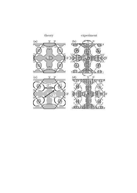
FIG. 6.: Theoretical and ARP Fermi surfaces of the clean (upper part) und the H-covered (lower part) W(110) surface. The solid (dotted) lines denote surface resonances or surface states which are localized by more than 60 % (30 %) in the MTs of the two top W layers. Shaded areas represent the (110) projected theoretical W bulk Fermi surface. The arrows $\overline{Q}^{\rm c,1}_{\rm exp}$ and $\overline{Q}^{\rm c,2}$ are the critical wave vectors found in HAS. The ARP data stem from Refs. [9, 17].

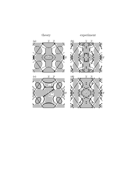
FIG. 7.: Theoretical Fermi surfaces of the (a) clean and (c) H-covered Mo (110) surface. Also presented are data points (+) which stem from an ARP study of the (b) clean and (d) H-covered Mo_0.95Re_0.05 (110) surface [50]. The presentation is equivalent to Fig. 6.

In Figs. 6 and 7 we report the calculated Fermi surfaces and compare them to experimental ones obtained by Kevan’s [9, 17] and Plummer’s [50] groups. Let us first focus on the theoretical results which are — as in the case of the surface geometries — again very similar for Mo and W.

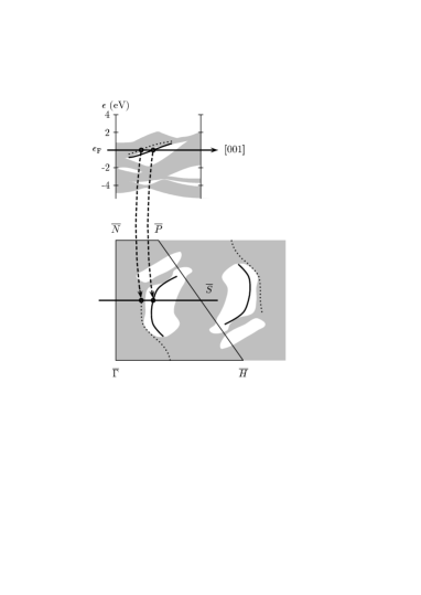
FIG. 8.: Hydrogen induced shift of the ($d_{3z^{2}-r^{2}},d_{xz}$) band at the Mo(110) surface. The upper part of the figure represents a one-dimensional cut through the two-dimensional surface bandstructure. Shaded areas illustrate the (110) projected bulk band structure. The dotted (solid) lines depict the position of the ($d_{3z^{2}-r^{2}},d_{xz}$) band for the clean (H-covered) surface. The arrows indicate how the bandstructure translates into the two-dimensional Fermi surface shown in the lower part. In Fig. 9 the charge density of the two states marked by the arrows is presented.

For both systems the H-adsorption induces the shift of a band with $(d_{3z^{2}-r^{2}},d_{xz})$ character to lower binding energies [49, 51]. This effect which is illustrated in Fig. 8 moves the Fermi line associated with this band into the band gap of the surface projected band structure. Subsequently, the respective states become true surface states. It is important to note that the band shift is due not to a hybridization between hydrogen orbitals and ($d_{3z^{2}-r^{2}},d_{xz}$) bands but to a hydrogen induced modification of the surface potential. The bonding states of the hydrogen-substrate interaction are about 5 eV below the Fermi energy and the anti-bonding states are 4 eV above. Therefore, they are not involved in this process which takes place at the Fermi level.

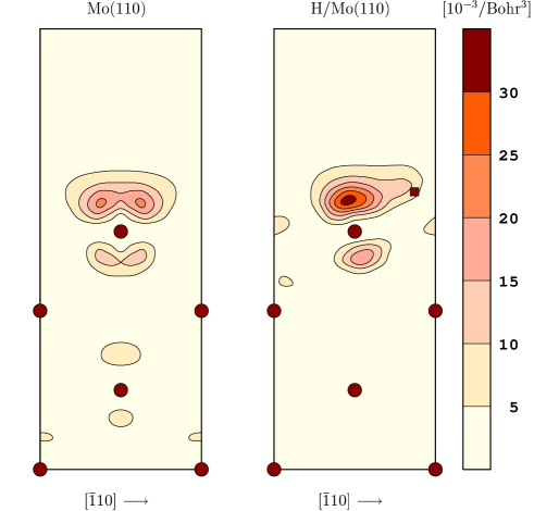
FIG. 9.: Charge density plot along the $(010)$ plane for Mo(110) and H/Mo(110): Shown are the two states marked in Fig. 8 by arrows. Only the plane-wave part of the wavefunctions is shown. The positions of the Mo atoms are marked by dots. The square represents the hydrogen atom in the hollow adsorption site.

TABLE III.: Theoretical Fermi surface nesting vectors compared to critical wavevectors obtained by HAS and HREELS experiments [2, 3, 7, 8].

direction	system	$|{\overline{Q}}^{\rm c}|\ \ [\mbox{\AA}^{-1}]$
		theory	experiment
$\overline{\Gamma H}\ \$	H/Mo(110)	0.86	0.90
	H/W(110)	0.96	0.95
$\overline{\Gamma S}\ \$	H/Mo(110)	1.23	1.22
	H/W(110)	1.22	1.22

The shifted $(d_{3z^{2}-r^{2}},d_{xz})$ band is characterized by a high density of states at the Fermi level. For the clean Mo(110) surface one finds that the ($d_{3z^{2}-r^{2}},d_{xz}$) band has a MT localization of $w^{\rm MT}\approx 30\%$. Due to the H-adsorption this value increases to more than 60%. This modification is also visible in the charge density plots in Fig. 9. More important, the new Fermi contour reveals pronounced nesting features. In Figs. 6c and 7c one sees the dramatic changes due to the H-induced shift. Segments of the two-dimensional Fermi contour of the ($d_{3z^{2}-r^{2}},d_{xz}$) band are now running parallel to $\overline{\Gamma N}$ and normal to $\overline{\Gamma S}$. There are two nesting vectors $\overline{Q}^{\rm c,1}$ and $\overline{Q}^{\rm c,2}$ which connect those segments in different parts of the SBZ. As can be seen in Table III they agree very well with the HAS measured critical wavevectors.

With respect to those nesting vectors our results contradict the photoemission studies by Kevan and coworkers [9, 16, 17, 52] which were depicted in Figs. 6b,d (for W) and Fig. 2 in Ref. [49] (for Mo). Apart from that Kevan’s and our data compare rather well. Therefore, it is difficult to give a plausible reason for the discrepancies. However, in view of the fact that for the clean surface the theoretical and experimental Fermi surfaces are in very good agreement and that our calculated Fermi nesting vectors agree very well with the HAS and HREELS anomalies we dared to suggest that those differences may be due to the already discussed problems within the experimental analysis [49]. We also note that recent ARP studies [50] of a related system which we present in Fig. 7 seem to support our conclusion. This experimental work deals with the (110) surface of the alloy Mo_0.95Re_0.05 but the surface physics of Mo_0.95Re_0.05 (110) and Mo (110) should be practically the same because in both cases the top layer consists only of Mo atoms. This assumption is also backed by test calculations where we simulated a Mo_0.95Tc_0.05 alloy be the virtual crystal approximation and found only minor quantitative changes.

From Figs. 7c and 7d it becomes clear that in particular for the important $(d_{3z^{2}-r^{2}},d_{xz})$ surface band, which was not seen by Kevan’s group, experiment and DFT now agree very well. There are however still differences: Theory predicts bands centered at $\overline{S}$ which are not seen by ARP whereas the band circle at $\overline{\Gamma}$ in Fig. 7d is only observed experimentally. Also, in the calculations we find an elliptical band centered at the $\overline{\Gamma}$ point whereas in ARP the same band has the shape of a rectangle. Those discrepancies are probably due to matrix elements of the photoemission process and to the inherent inaccuracies in theory and experiment which we mentioned above. Nevertheless, the theoretical results are encouraging because they provide strong evidence for a link between the HAS anomalies and the Fermi surfaces.

C Vibrational Properties

The study of the electronic structure revealed pronounced nesting features for the H-covered surfaces. At this point, the following question arises: How does the surface react to this apparent electronic instability? At the $\bf k$ vectors of the Fermi surface nesting the coupling between electrons and phonons is expected to become significant which implies a possible breakdown of the Born-Oppenheimer approximation. This leads to a softening of the related phonons. If the electron-phonon coupling is strong and the energetic cost of a surface distortion is small the nesting could even trigger a reconstruction combined with the build-up of a charge-density wave as in the case of the (001) surfaces of W [10] and Mo [11]. Then, at the reconstructed surface, the Born-Oppenheimer approximation is valid again. It is clear that one needs to perform frozen-phonon calculations in order to determine the actual strength of the electron-phonon coupling and the resulting phonon softening [18].

The experimental vibrational spectra of the (110) surfaces of Mo and W show two distinct reactions to the adsorption of hydrogen. Along $\overline{\Gamma H}$ and $\overline{\Gamma S}$ the H-adsorption induces a softening of the Rayleigh and (to a smaller amount) of the longitudinal wave [53] while a stiffening of these modes is observed along $\overline{\Gamma N}$. Our goal is to investigate both effects theoretically.

We use an enlarged surface unit cell together with a five layer slab. The plane-wave cutoff for the wavefunctions is reduced to $\frac{\hbar^{2}}{2m}(K^{\rm wf})^{2}=10$ Ry (see test caculations in the Appendix 3). The geometries are defined by the five layer relaxation parameters presented in Table II. Some relaxation parameters, i.e., $\Delta d_{ij}$, change considerably when we perform a calculation with a slab of five instead of seven or nine metal layers. We note, however, that the values of the critical wavevectors and the position of the hydrogen with respect to the substrate surface are practically insensitive to the thickness of the slab. This indicates that the physical properties we are interested in, e.g. the nesting features, are well localized surface phenomena and that the results of our five layer slab studies can be trusted. As shown in Appendix 3 for the $\overline{S}$ point phonon the calculated frequencies are relatively insensitive to the the SBZ $\bf k_{\|}$ point sampling, and we conclude that a uniform mesh of 56 points is sufficient for the present study.

Being zone boundary phonons in the Rayleigh waves at $\overline{S}$ and $\overline{N}$ the displacements of the surface atoms are along the direction normal to the surface. Moreover, the vibrations are strongly localized in the surface region. We assume that even with hydrogen adsorbed the coupling to modes parallel to the surface is small. Therefore, we can confine our study to the vibrational components normal to the surface. Besides the first substrate layer we also include the vibrations of the second layer in our calculations. Due to the small mass the hydrogen atom follows the substrate vibrations adiabatically. In the calculations this adsorbate relaxation lowers the distortion energy by several meV and thus reduces the phonon energy significantly. Therefore, all phonon frequencies are calculated for a fully relaxed hydrogen adsorbate.

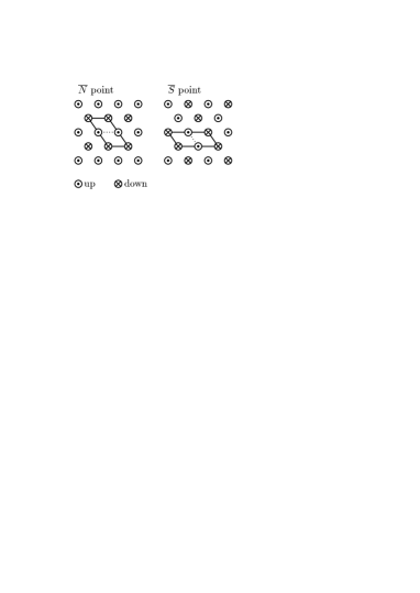
FIG. 10.: Distortion pattern of the atoms of the top metal layer for the Rayleigh phonons at the symmetry points $\overline{S}$ and $\overline{N}$.

For the study of the vibrational properties of the systems we displace the substrate atoms in the surface (according to Fig. 10), relax the hydrogen atom, and calculate the resulting atomic forces. The same is done for the atoms in the subsurface layer. From a third-order fit to the calculated forces for five different displacement steps between 0% and 5% of the lattice constant we obtain the matrix elements of the dynamical matrix and then via diagonalization the respective phonon energies. The calculated frequencies are collected in Table IV. At the $\overline{N}$ point our results reproduce the experimentally observed increase of the Rayleigh-wave frequency as hydrogen is adsorbed.

TABLE IV.: Comparison of calculated frozen-phonon energies and experimental values obtained by HAS [2, 3] and HREELS [8]. The theoretical phonon energies are obtained using a five-layer slab. Their numerical accuracy is about $\pm 5\%$, i.e., $\pm 1$ meV.

phonon	system	$E^{\rm ph}$  [meV]
		theory	experiment
$\bar{N}$	W (110)	15.4	14.5
	H/W (110)	17.6	17.0
$\overline{S}$	Mo (110)	22.7	$\sim$21
	H/Mo (110)	17.2	$<$16
	W (110)	18.3	16.1
	H/W (110)	12.0	11.0

FIG. 11.: Schematic representation of the mechanism which causes the Kohn anomaly of the H/Mo(110) and H/W(110). Shown is the bandstructure along $\overline{S\Gamma S}$ parallel to the nesting vector $\overline{Q}^{c,2}$ in Figs. 6c and 7c. The form of the ($d_{3z^{2}-r^{2}},d_{xz}$) band is indicated by dashed lines. See text for a detailed description.

At the ${\overline{S}}$ point we find that the strong coupling to electronic states at the Fermi level leads to a lowering of the phonon energy in good agreement with the experimental results. In Figs. 11a-c we schematically illustrate the mechanism which is responsible for this effect. It is, in fact, a text-book example of a Kohn anomaly due to Fermi-surface nesting [54, 55]: (a) Within the unperturbated system the ($d_{3z^{2}-r^{2}},d_{xz}$) band cuts the Fermi level exactly midway between $\overline{\Gamma}$ and $\overline{S}$. (b-c) The nuclear distortion associated with the $\overline{S}$-point phonon modifies the surface potential and hence removes the degeneracy at the backfolded zone boundary point $\overline{S^{\prime}}$.

FIG. 12.: H/W(110): Band gap $\Delta$ induced by a $\overline{S}$ point frozen-phonon distortion. Shown are the KS eigenvalues of the ($d_{3z^{2}-r^{2}},d_{xz}$) band at the $\overline{S^{\prime}}$ point versus the amplitude of the atomic distortion $t_{1z}$ of the first substrate layer.

The occupied states are shifted to lower energies (see Fig. 12). This amounts to a negative contribution of the electronic band structure energy to the total energy and thus a lowering of the phonon energy.

A frozen-phonon study for the second nesting vector along $\overline{\Gamma H}$ is not performed because the respective $\overline{Q}^{\rm c,1}$ is highly non-commensurate. Thus, such a calculation would be very expensive. However, since the character of the $(d_{3z^{2}-r^{2}},d_{xz})$ band does not change when shifting from the $\overline{\Gamma S}$ to the $\overline{\Gamma H}$ nesting we expect similar results; this was recently confirmed by Bungaro [56] within the framework of a perturbation theory.

The calculation of the electron-phonon interaction at the Mo (110) and W (110) surfaces and its change due to hydrogen adsorption pinpoints the phonon character of the small anomaly $\omega_{2}$ and identifies the interplay between the electronic structure and the vibrational spectra of the transition metal surfaces. Thus, our results clearly support the interpretation that the small dip observed by both HAS and HREELS is due to a Kohn anomaly. Furthermore, we find that the electron-phonon coupling is not strong enough to induce a stable reconstruction. Thus, the system remains in a somewhat limbo-like state.

D Electron-Hole Excitations

For the deep and narrow anomaly $\omega_{1}$ the interpretation appears to be less straightforward. It is particularly puzzling that it is only seen in the HAS spectra and not in HREELS. This difference. together with the above noted “limbo state” of the surface yield the clue to our present interpretation. At first, it is necessary to understand the nature of rare-gas atom scattering.

FIG. 13.: Schematic illustration of the scattering of He atoms (HAS, upper part) and electrons (HREELS, lower part) at a metal surface (from Ref. [57]).

In a recent study we found that those scattering processes are significantly more complicated (and more interesting) than hitherto assumed [58]: The reflection of the He atom happens in front of the surface at a distance of 2–3 Å. This is illustrated in Fig. 13. More important, it is not the total electron density of the substrate surface which determines the interaction but the electronic wavefunctions close to the Fermi level. In the case of the H/W (110) and H/Mo (110) systems it is thus plausible to assume that the He atom couples directly to the $(d_{3z^{2}-r^{2}},d_{xz})$ surface states mentioned above and excites electron-hole pairs. By contrast, the electrons in HREELS scatter at the atomic cores and interact only weakly with the electron density at the surface.

In order to analyze the spectrum of those excitations as seen by HAS in some more detail we evaluate the local density of electron-hole excitations

$$P({\bf q_{\|}},\hbar\omega) = \int_{\rm SBZ}d{\bf k_{\|}}\ w_{\bf k_{\|}+\bf q_{\|}}w_{\bf k_{\|}}\ (f_{\bf k_{\|}+\bf q_{\|}}-f_{\bf k_{\|}})$$ (7)

$$\hskip 28.45274pt\times\delta\left(\epsilon_{\bf k_{\|}+\bf q_{\|}}-\epsilon_{\bf k_{\|}}-\hbar\omega\right)$$

which is a measure of the probability that a He atom looses the energy $\hbar\omega$ and the momentum $\bf q_{\|}$ when interacting with the surface elctron density. In our approach we use all eigenvalues $\epsilon_{\bf k_{\|}}$ and occupation numbers $f_{\bf k_{\|}}$ obtained via a nine-layer slab calculations. In order to refer to HAS we take into account the localization $w_{\bf k_{\|}}$ of the respective state at a distance of 2.5 Å in front of the substrate surface.

FIG. 14.: Contour plot of the local probability function $P({\bf q_{\|}},\hbar\omega)$ of Mo (110) and H/Mo (110) calculated for $\hbar\omega=0.5$ mRy $\approx 6.8$ meV. The dashed line represents a value of 3 arbitrary units while each full line denotes an additional increase by 1 arbitrary units (with increasing line width). The positions of the HAS measured anomalies within the SBZ are indicated by dots.

FIG. 15.: Contour plot of the local probability function $P({\bf q_{\|}},\hbar\omega)$ of W (110) and H/W (110) calculated for $\hbar\omega=0.5$ mRy $\approx 6.8$ meV. Notation equivalent to Fig. 14.

The results obtained for Mo (110) and H/Mo (110) are presented in Figs. 14. For the clean surface we find that the intensity of the electron-hole excitations decreases continuously as we move away from the $\overline{\Gamma}$ point towards the zone boundaries. This relatively smooth behavior of the susceptibility is modified considerably when hydrogen is adsorbed on the clean surface: Pronounced peaks appear, in particular one which stretches from the $\overline{\Gamma H}$ line through the SBZ to the symmetry point $\overline{S}$. This is in excellent agreement with the HAS results (see also Fig. 2). Also, there is a peak located at the upper half of the $\overline{\Gamma N}$ symmetry line. It cannot be associated with an anomaly in the HAS spectrum. This result may be due to the fact that selection rules or matrix elements for the interaction between the scattering He atoms and the electron-hole excitations are not considered in $P({\bf k},\hbar\omega)$. In Fig. 15 the respective data for the clean and H-covered W (110) surfaces are displayed. In general, our findings are in agreement with the experimental results of Lüdecke and Hulpke that the anomaly stretches through the SBZ. However, we do not support the idea of a fully one-dimensional nesting mechanism with a constant [001]-component of the critical wave vector as depicted in Fig. 2.

In view of the simplicity of our approach, the calculated spectrum of electron-hole excitations as predicted by $P({\bf q},\hbar\omega)$ seems to be well-connected to the HAS measurements. Moreover, it is surprising how detailed the Fermi-surface nesting (compare to Figs. 6c and 7c) is still present at a (rather large) distance from the surface. In fact, if the localization $w_{\bf k_{\|}}$ were not included into the calculations or if it were taken closer to the surface the H-induced peaks would be hidden in the background noise of other electron-hole excitations. The clear image in Figs. 14 and 15 only appears if we take the position of the classical turning point into account.

To our knowledge these are the first theoretical studies of the rare-gas atom scattering spectrum using a first-principles electronic bandstructure. Our findings support the earlier suggestion [49] that the giant indentations, seen only in HAS, are due to the excitation of electron-hole pairs. In HREELS such excitations are less likely, and thus the strong anomaly remains invisible.

IV Summary and Outlook

In conclusion, the major results of our work are as follows: We demonstrate that for both W (110) and Mo (110) the $(1\times 1)$ surface geometry is stable upon hydrogen adsorption. There is no evidence for a pronounced H-induced top-layer-shift reconstruction, a result confirmed by a recent LEED analysis [47, 48]. Also, we give a consistent explanation for the H-induced anomalies in the HAS spectra of W (110) and Mo (110). The H-adsorption induces surface states of $(d_{3z^{2}-r^{2}},d_{xz})$ character that show pronounced Fermi-surface nesting. The modestly deep anomaly is identified as a Kohn anomaly due to those nesting features [49, 51, 18]. For an understanding of the huge dip we stress that the scattering of rare-gas atoms is crucially influenced by interactions with substrate surface wavefunctions at the classical turning point [58]. Assuming that the He atom couples efficiently to the H-induced surface states on H/W (110) and H/Mo (110) we therefore conclude that the deep HAS anomaly is predominantly caused by a direct excitation of electron-hole pairs during the scattering process.

We hope that our calculations and interpretations stimulate additional theoretical and experimental work: For instance, it is highly important to better understand the details of rare-gas atom scattering processes at “real” surfaces. Also, the liquid-like behavior of the H-adatoms observed in the HREELS measurements [8] remains an unresolved puzzle. One would also like to know whether the HAS and HREELS spectra of the Mo_0.95Re_0.05 (110) alloy system reveal H-induced anomalies as expected. Finally, we call for a new ARP study of the clean and H-covered Mo (110) and W (110) surfaces in order to experimentally identify the Fermi surface. We also note that scattering experiments with atoms or molecules like Ne or H₂ might provide additional insight into the interesting behavior of these surfaces.

Test Calculations

1 Bulk

TABLE V.: Theoretically and experimentally obtained crystal parameters for Mo and W. The percentage deviations from experiment are given in parentheses. The results of this work are calculated non-relativistically (N) and scalar-relativistically (R). Also, the different XC potentials used in the theoretical studies are given: Wigner [59] (W37), Barth and Hedin [60] (BH72), and Ceperley and Alder [21] (CA80) parameterized by Perdew and Zunger [22]. The abreviation “NL-PP” stands for “non-local pseudo-potential” method. All theoretical numbers ignore the influence of zero-point vibrations.

metal	method	XC	$a_{0}$ [Å]	$B_{0}$ [MBar]
Mo	experimenta		3.148	2.608
	NL-PPb	BH72	3.152 (+0.1)	3.05 (15.5)
	LAPWc	BH72	3.131 ($-$0.5)	2.91 (11.6)
	this work (N)	CA80	3.126 ($-$0.7)	2.88 (10.4)
	this work (R)	CA80	3.115 ($-$1.1)	2.89 (10.8)
W	experimentd		3.163	3.23
	NL-PPb	BH72	3.173 (+0.3)	3.45 (6.8)
	LAPWe	W34	3.149 ($-$0.4)	3.46 (7.1)
	LAPWc	BH72	3.162 ($\pm$0.0)	3.40 (5.3)
	this work (N)	CA80	3.194 ($+1.0$)	2.92 (–9.6)
	this work (R)	CA80	3.137 ($-0.8$)	3.37 (4.3)

In Table V we list the calculated equilibrium lattice constants $a_{0}$ and the bulk moduli $B_{0}\equiv-V\partial^{2}E^{\rm tot}/\partial^{2}V$, and compare them to published results from experiment and theory. Our values were obtained using the LAPW parameter setting presented in Table I.

2 Surfaces

a Test System

The focus of this paper lies on the Mo(110) and W(110) surfaces. In order to test the numerical accuracy of our calculations for such systems it is important to go beyond typical tests for the crystal bulk. For instance, we need to know the error bars for atomic geometries obtained via forces as compared to a pure total energy calculation. Five- and more-layer systems are not suitable and in fact for most cases also not necessary for such a detailed study. Therefore, questions refering to the size of the vacuum region, to the accuracy of the directly calculated LAPW forces, and to the appropriate wavefunction cutoff will be answered by studying a simple Mo(110) double-layer slab system. Starting from the LAPW parameter set listed in Table I we vary one parameter and study its influence on the evaluated total energy and the atomic force. These quantities are calculated with respect to the inter-layer distance $z$. Again, we note that we are interested not in the physics of this double-layer system but in the accuracy and the convergence of our method. Therefore, the calculations are done using just four $\bf k_{\|}$ points within the SBZ.

Employing a least-square fit which has the form of a Morse potential [65]

$$E^{\rm tot}(z)=D\left[1-{\rm e}^{-\beta(z-d-d_{0})}\right]^{2}$$ (8)

we calculate the equilibrium relaxation parameter $d$. Here, $d_{0}$ represents (110) layer distance in the bcc crystal. Additionally, the vibrational properties are of considerable interest. From the Morse parameters $D$ and $\beta$ one extracts the oscillator frequency by using the expression

$$\omega^{2}=\frac{4D\beta}{M_{I}}$$ (9)

where the atomic masses $M_{I}$ are those of the Mo and W nuclei. A corresponding fit is also employed for the directly calculated forces normal to the (110) surface:

$$F(z) = -\frac{dE^{\rm tot}(z)}{dz}$$ (10)

$$= -2\tilde{D}\tilde{\beta}\left[{\rm e}^{-2\tilde{\beta}(z-\tilde{d}-d_{0})}-{\rm e}^{-\tilde{\beta}(z-\tilde{d}-d_{0})}\right]\quad.$$ (11)

This enables a quantitative study of the accuracy of the evaluated LAPW forces with respect to the total energy $E^{\rm tot}(z)$. Within the Tables VI–IX the two alternatives are marked by “F” (force) and “E” (energy).

We consider a calculation to be converged if the relaxation parameter $d$ and the frequency $\omega$ differ by less the $\Delta d=0.25\%d^{\rm conv}\approx 0.005$ Å and $\hbar\Delta\omega=\hbar 5\%\omega^{\rm conv}\approx 2$ meV from the fully converged results $d^{\rm conv}$ and $\omega^{\rm conv}$. In the following discussion we focus on these two quantities $d$ and $\omega$. They provide detailed information about the accuracy of structure-optimization and frozen-phonon calculations performed in this paper.

b Vacuum Size

TABLE VI.: Mo(110) double-layer: Morse parameter $d$ and the energy $\hbar\omega$ versus the number of vacuum layers. The arrow indicates the parameter choice which yields converged results.

number	$d$ [$\%d_{0}$]		$\hbar\omega$ [meV]
of layers	E	F	E	F
2	–1.7	–2.1	36.5	35.3
3	–1.7	–2.1	36.7	35.2
$\Rightarrow$ 4	–2.0	–2.4	37.3	35.6
5	–2.1	–2.4	37.4	35.7
6	–2.0	–2.3	36.9	35.4

The first set of test calculations serves to determine the appropriate size of the vacuum region. The results presented in Table VI show that an equivalent of four substrate layers ($\hat{=}$ 8.8 Å) is sufficient to decouple the two substrate surfaces accross the vacuum. Both relaxation parameter $d$ and the frequency $\omega$ vary only within the given error range upon further increasing the vacuum region.

c LAPW Parameters

TABLE VII.: Mo(110) double-layer: Variation of the wavefunction cutoff parameter $\frac{\hbar^{2}}{2m}(K^{\rm wf})^{2}$. The notation is equivalent to Table VI.

$\frac{\hbar^{2}}{2m}(K^{\rm wf})^{2}$	$d$ [$\%d_{0}$]		$\hbar\omega$ [meV]
[Ry]	E	F	E	F
9	–0.5	–1.0	35.0	33.4
10	–1.5	–2.1	36.0	34.6
11	–1.6	–2.2	36.1	35.2
$\Rightarrow$ 12	–2.0	–2.4	37.3	35.6
13	–1.9	–2.2	37.1	35.5
14	–1.9	–2.1	36.5	35.4

Another important parameter is the wavefunction energy cutoff $\frac{\hbar^{2}}{2m}(K^{\rm wf})^{2}$. It has a decisive influence on the computer time. With respect to the structure parameter $d$ our results in Table VII indicate that the smallest possible value is $\frac{\hbar^{2}}{2m}(K^{\rm wf})^{2}=12\,$Ry. However, for $\hbar\omega$ already a calculation with $\frac{\hbar^{2}}{2m}(K^{\rm wf})^{2}=10\,$Ry provides converged results.

TABLE VIII.: Mo(110) double-layer: Variation the potential paremters $\frac{\hbar^{2}}{2m}(G^{\rm pot})^{2}$ and $l^{\rm pot}$. The notation is equivalent to Table VI.

$\frac{\hbar^{2}}{2m}(G^{\rm pot})^{2}$	$d$ [$\%d_{0}$]		$\hbar\omega$ [meV]
[Ry]	E	F	E	F
64	–2.0	–2.3	37.3	35.6
81	–1.9	–2.3	36.6	35.5
$\Rightarrow$ 100	–2.0	–2.4	37.3	35.6
121	–1.9	–2.3	37.0	35.6
144	–1.9	–2.3	37.0	35.6

$l^{\rm pot}$	$d$ [$\%d_{0}$]		$\hbar\omega$ [meV]
	E	F	E	F
2	–1.9	–1.7	37.5	34.6
$\Rightarrow$ 3	–2.0	–2.4	37.3	35.6
4	–2.0	–2.5	37.1	35.2
5	–2.1	–2.6	37.1	35.3

The two potential parameters $\frac{\hbar^{2}}{2m}(G^{\rm pot})^{2}$ and $l^{\rm pot}$ are of little influence on the calculated quantities. This can be seen in Table VIII. The values of the relaxation parameter $d$ and the frequency $\omega$ remain relatively stable within the parameter range 64 Ry $<\frac{\hbar^{2}}{2m}(G^{\rm pot})^{2}<144\,$Ry. Both quantities are more sensitive to changes in the $(l,m)$ expansion of the MT potential. However, a value of $l^{\rm pot}=3$ seems to be sufficient.

In general we note that energy (E) and force (F) calculations demonstrate a similar convergence behavior. However, the magnitude of the relaxation in the force calculations is overestimated by about $\Delta d=0.5\%d^{\rm conv}\approx 0.01\,$Å; for the frequencies one finds a deviation of about $\hbar\Delta\omega=5\,\%\hbar\omega^{\rm conv}\approx 1.8$ meV from the converged total energy values. Those differences are probably due to numerical inaccuracies in the force calculation.

d $\bf k_{\|}$ Point Set

Similar calculations for a W(110) double-layer system lead to a converged LAPW parameter set which is comparable to the one obtained for Mo. Only the MT potential parameter $l^{\rm pot}$ has to be chosen higher: $l^{\rm pot}=4$. slightly different. The agreement between force and total energy calculations ($\Delta d=1\%d^{\rm conv}\approx 0.02$ Å and $\Delta\omega=5\%\omega^{\rm conv}$) is nearly as good as in the case of Mo. The following calculation is aimed to determine a two-dimensional $\bf k_{\|}$-point set which can be used for the calculation of the atomic and electronic structure of Mo (110) and W (110) surfaces (see Table IX).

TABLE IX.: W(110) double-layer: Accuracy of the calculation in dependence of the number of $\bf k_{\|}$-points for the (a) valence electrons and (b) semicore electrons. The respective fixed $\bf k_{\|}$-point set is made up by one special $\bf k_{\|}$-point in the irreducible part of the SBZ [46]. The arrows indicate the converged $\bf k_{\|}$-point set used for the (110) surface calculations. The notation is equivalent to Table VI.

(a) valence electrons $\#$ $d$ [$\%d_{0}$] $\hbar\omega$ [meV] $\bf k_{\|}$-points E F E F 36 –8.5 –9.5 20.5 21.1 49 –9.0 –10.1 23.8 23.1 $\Rightarrow$ 64 –8.4 –9.3 19.2 20.3 81 –8.4 –9.4 18.9 20.4

(b) semicore electrons $\#$ $d$ [$\%d_{0}$] $\hbar\omega$ [meV] $\bf k_{\|}$-points E F E F 4 –1.0 –1.8 27.4 26.2 $\Rightarrow$ 9 –1.0 –1.9 27.4 26.2 16 –1.0 –1.9 27.3 26.2 25 –1.0 –1.9 27.4 26.2 36 –1.0 –1.9 27.4 26.2

Because of the size of (110) surface slab systems it is important to keep the number of $\bf k_{\|}$-points as small as possible. For the calculations we use the LAPW parameter set given in Table I and vary the $\bf k_{\|}$-point set for either the valence or the semicore electrons. These sets always consist of uniform two-dimensional point meshes. Converged results are obtained by using 64 $\bf k_{\|}$-points for the valence and 9 $\bf k_{\|}$-points for the semicore electrons.

3 Phonons

a LAPW parameter

Our final series of tests is meant to determine the accuracy of the frozen-phonon calculation. In order to keep the computer time for those elaborate calculations within pleasant limits one has to keep the number of $\bf k_{\|}$-points and basis functions as small as possible. As a sample case we study the $\overline{S}$ point Rayleigh phonon of the H/Mo (110) system.

The calculations are performed as follows: We distort the atoms of the first substrate layer by $t_{1z}(\overline{S})=0.08\,$Å  according to the pattern in Fig. 10 and determine the total energy and force changes $\Delta E^{\rm tot}$ and $\Delta F_{1z}$. These quantities have the same convergence behavior as the phonon frequencies: Therefore, if $\Delta E^{\rm tot}$ and $\Delta F_{1z}$ are stable with respect to a particular LAPW parameter so are the phonon frequencies. Converged results for Mo as well as for W are obtained by using the following setting: wavefunction plane-wave cutoff $\frac{\hbar^{2}}{2m}(K^{\rm wf})^{2}=10\,$Ry; $l^{\rm pot}=3$ for the $(l,m)$ expansion of the MT potential; uniform $\bf k_{\|}$-point mesh consisting of 56 points; five substrate layers; a vacuum region equivalent to four substrate layers; XC potential from Refs. [21, 22].

b $\bf k_{\|}$ Point Mesh

In order to accurately describe the electronic structure and hence the electron-phonon coupling for the $\overline{S}$ point phonon one has to provide a detailed $\bf k_{\|}$-point set. For instance, for the study of the $(2\times 1)$ reconstructions of the diamond (111) surface Vanderbilt and Louie employ a $\bf k_{\|}$-point mesh which becomes logarithmically denser close to the zone boundary [66]. One cannot rely on the results for the two Mo (110) and W (110) double-layer slabs in Section 2 d because in these systems nesting effects are totally unimportant.

TABLE X.: Frozen-phonon distortion for H/Mo(110): Change of the total energy $\Delta E^{\rm tot}$ and the force $\Delta F_{1z}$ versus the number of $\bf k_{\|}$-points. All $\bf k_{\|}$-point sets are uniform meshes which include the symmetry point $\overline{S^{\prime}}$ of the backfolded SBZ (see Fig. 11). Given are also the calculated values for the clean Mo(110) surface (with 56 $\bf k_{\|}$-points).

# $\bf k_{\|}$-points	$\Delta E^{\rm tot}$ [meV]	$\Delta F_{1z}$ [meV/Å]
16	110	672
56	136	756
80	144	797
120	135	790
232	136	777
clean	161	938

We perform tests for the H/Mo(110) system using up to 232 $\bf k_{\|}$-points in the SBZ and find that a uniform $\bf k_{\|}$-point mesh of 56 points is sufficient in order to obtain converged results (see Table X). For all those frozen-phonon calculations the Monkhorst-Pack $\bf k_{\|}$-point meshes [46] are shifted in order to include the $\overline{S}^{\prime}$ point of the $(1\times 1)$ unit cell (see Fig. 11). For the $\bf k_{\|}$-point summation we employ a Fermi smearing of $k_{\rm B}T_{\rm el}\approx 68$ meV. Only for the 232 $\bf k_{\|}$-point calculation listed in Table X a smaller value of $k_{\rm B}T_{\rm el}\approx 14$ meV is used. However, this parameter is apparently uncritical because the energies are obtained for the $k_{\rm B}T_{\rm el}\leftarrow 0$ K limit as discussed in Ref. [42].

c Basisfunctions

Next, we check whether the results are sensitive to an increase in the wavefunction cutoff, i.e., whether the chosen value $\frac{\hbar^{2}}{2m}(K^{\rm wf})^{2}=10\,$Ry is large enough.

TABLE XI.: Frozen-phonon distortion for H/Mo(110): Change of the total energy $\Delta E^{\rm tot}$ and the force $\Delta F_{1z}$ with respect to the wavefunction plane-wave cutoff $\frac{\hbar^{2}}{2m}(K^{\rm wf})^{2}$.

$\frac{\hbar^{2}}{2m}(K^{\rm wf})^{2}$ [Ry]	$\Delta E^{\rm tot}$ [meV]	$\Delta F_{1z}$ [meV/Å]
10	136	756
12	137	767

The data listed in Table XI demonstrates that this is indeed the case. The results remain stable for the higher cutoff $\frac{\hbar^{2}}{2m}(K^{\rm wf})^{2}=12\,$Ry.

d LDA versus GGA

TABLE XII.: Frozen-phonon distortion for H/Mo(110): Variation of the XC potential: LDA [21, 22], GGA [44].

XC Potential	$\Delta E^{\rm tot}$ [meV]	$\Delta F_{1z}$ [meV/Å]
LDA	136	756
GGA	141	764

For some systems involving hydrogen the results of a total energy calculation are not reliable if the LDA is used. In those cases the bonding — especially between hydrogen atoms — is only described accurately if gradient corrections are considered [67]. In Table XII we compare results obtained with the generalized gradient approximation (GGA) [44, 45] and those found within the LDA. The latter is identical with the 56 $\bf k_{\|}$-point calculation in Table X. There, the XC potential of Cepereley and Alder [21] parametrized by Perdew and Zunger [22] is used. The small energy and force differences of 5 meV and 8 meV/Å, respectively, clearly shows that our adsorbate systems are rather insensible to the XC formalism chosen.

REFERENCES

- [1] M. Balden, S. Lehwald, and H. Ibach, Phys. Rev. B53, 7479 (1996).
- [2] E. Hulpke and J. Lüdecke, Surf. Sci. 272, 289 (1992).
- [3] J. Lüdecke, Ph.D. thesis (Universität Göttingen, 1994).
- [4] E. Hulpke and J. Lüdecke, Phys. Rev. Lett.68, 2846 (1992).
- [5] E. Hulpke and J. Lüdecke, Surf. Sci. 287/288, 837 (1993).
- [6] E. Hulpke and J. Lüdecke, J. Electron. Spectr. Relat. Phenom. 64/65, 641 (1993).
- [7] M. Balden, S. Lehwald, and H. Ibach, Surf. Sci. 307/309, 1141 (1994).
- [8] M. Balden, S. Lehwald, H. Ibach, and D. L. Mills, Phys. Rev. Lett.73, 854 (1994)
- [9] R. H. Gaylord, K. H. Jeong, and S. D. Kevan, Phys. Rev. Lett.62, 2036 (1989).
- [10] H.-J. Ernst, E. Hulpke, and J. P. Toennies, Phys. Rev. B46, 16081 (1992).
- [11] E. Hulpke and D.-M. Smilgies, Phys. Rev. B40, 1338 (1989).
- [12] X. W. Wang and W. Weber, Phys. Rev. Lett.58, 1452 (1987).
- [13] X. W. Wang, C. T. Chan, K.-M. Ho, and W. Weber, Phys. Rev. Lett.60, 2066 (1988).
- [14] K. E. Smith, G. S. Elliott, and S. D. Kevan, Phys. Rev. B42, 5385 (1990).
- [15] J. W. Chung, K. S. Shin, D. H. Baek, C. Y. Kim, H. W. Kim, S. K. Lee, C. Y. Park, S. C. Hong, T. Kinoshita, M. Watanabe, A. Kakizaki, and T. Ishii, Phys. Rev. Lett.69, 2228 (1992).
- [16] K. H. Jeong, R. H. Gaylord, and S. D. Kevan, Phys. Rev. B39, 2973 (1989).
- [17] K. H. Jeong, R. H. Gaylord, and S. D. Kevan, J. Vac. Sci. Technol. A 7(3), 2199 (1989).
- [18] B. Kohler, P. Ruggerone, M. Scheffler, and E. Tosatti, to be published in Z. Chem. Phys. (1996).
- [19] J. W. Chung, S. C. Ying, and P. J. Estrup, Phys. Rev. Lett.56, 749 (1986).
- [20] M. Altman, J. W. Chung, P. J. Estrup, J. M. Kosterlitz, J. Prybyla, D. Sahu, and S. C. Ying, J. Vac. Sci. Technol. A 5, 1045 (1987).
- [21] D. M. Ceperley and B. J. Alder, Phys. Rev. Lett.45, 566 (1980).
- [22] J. P. Perdew and A. Zunger, Phys. Rev. B23, 5048 (1981).
- [23] P. Blaha, K. Schwarz, and P. Herzig, Phys. Rev. Lett.54, 1192 (1985).
- [24] P. Blaha, K. Schwarz, P. Sorantin, and S. B. Trickey, Comput. Phys. Commun. 59, 399 (1990).
-
[25]
P. Blaha, K. Schwarz, and R. Augustyn,
WIEN93(Technische Universität Wien, 1993). - [26] R. Yu, D. Singh, and H. Krakauer, Phys. Rev. B43, 6411 (1991).
- [27] B. Kohler, S. Wilke, M. Scheffler, R. Kouba, and C. Ambrosch-Draxl, Comput. Phys. Commun. 94, 31 (1996).
- [28] R. Stumpf and M. Scheffler, Comput. Phys. Commun. 79, 447 (1994); Phys. Rev. B53, 4958 (1996).
- [29] D. D. Koelling, J. Phys. Chem. Solids 33, 1335 (1972).
- [30] D. D. Koelling and G. O. Arbman, J. Phys. F 5, 2041 (1975).
- [31] O. K. Andersen, Solid State Commun. 13, 133 (1973).
- [32] O. K. Andersen, Phys. Rev. B12, 3060 (1975).
- [33] E. Wimmer, H. Krakauer, M. Weinert, and A. J. Freeman, Phys. Rev. B24, 864 (1981).
- [34] H. J. F. Jansen, and A. J. Freeman, Phys. Rev. B30, 561 (1984).
- [35] L. F. Mattheiss and D. R. Hamann, Phys. Rev. B33, 823 (1986).
- [36] D. J. Singh, Planewaves, pseudopotentials, and the LAPW method (Kluwer Academic, Boston, 1994).
- [37] S. Blügel, Ph.D. thesis (RWTH Aachen, 1988).
- [38] J. M. Soler and A. R. Williams, Phys. Rev. B40, 1560 (1989).
- [39] J. C. Slater, Phys. Rev. 51, 846 (1937).
- [40] J. C. Slater, Advances in Quantum Chemistry 1, 35 (1964).
- [41] T. L. Loucks, Augmented Plane Wave Method (Benjamin, New York, 1967).
- [42] J. Neugebauer and M. Scheffler, Phys. Rev. B46, 16067 (1992).
- [43] P. Alippi and M. Scheffler, to be published.
- [44] J. P. Perdew and Y. Wang, Phys. Rev. B45, 13244 (1992).
- [45] J. P. Perdew, J. A. Chevary, S. H. Vosko, K. A. Jackson, M. R. Pederson, D. J. Singh, and C. Fiolhais, Phys. Rev. B46, 6671 (1992).
- [46] H. J. Monkhorst and J. D. Pack, Phys. Rev. B13, 5188 (1976).
- [47] M. Arnold, L. Hammer, K. Heinz, B. Kohler, and M. Scheffler, to be published.
- [48] M. Arnold, private communication.
- [49] B. Kohler, P. Ruggerone, S. Wilke, and M. Scheffler, Phys. Rev. Lett.74, 1387 (1995).
- [50] M. Okada, A. P. Baddorf, D. M. Zehner, and E. W. Plummer, Surf. Sci., in print.
- [51] P. Ruggerone, B. Kohler, S. Wilke, and M. Scheffler, Electronic Surface and Interface States on Metallic Systems, eds. E. Bertel and M. Donath (World Scientific, Singapore, 1995), p. 113.
- [52] K. H. Jeong, R. H. Gaylord, and S. D. Kevan, Phys. Rev. B38, 10302 (1988).
- [53] M. Balden, private communication.
- [54] A. B. Migdal, Sov. Phys. JETP 34, 996 (1958).
- [55] W. Kohn, Phys. Rev. Lett.2, 393 (1959).
- [56] C. Bungaro, Ph.D. thesis (SISSA, Trieste, 1995).
- [57] J. P. Toennies, Springer Series of Surface Science Bd. 21 eds. W. Kresse and F. de Wette (Springer, Berlin, 1991).
- [58] M. Petersen, S. Wilke, P. Ruggerone, B. Kohler, and M. Scheffler, Phys. Rev. Lett.76, 995 (1996).
- [59] E. Wigner, Phys. Rev. 46, 1002 (1934).
- [60] U. von Barth and L. Hedin, Solid State Commun. 5, 1629 (1972).
- [61] K. W. Katahara, M. H. Manghnani, and E. S. Fisher, J. Phys. F 9, 773 (1979).
- [62] A. Zunger and M. L. Cohen, Phys. Rev. B19, 568 (1979).
- [63] J. S. Shah and M. E. Straumanis, J. Appl. Phys. 42, 3288 (1971).
- [64] C. Kittel, Introduction to Solid State Physics (Wiley, New York, 1976).
- [65] P. M. Morse, Phys. Rev. 34, 57 (1929).
- [66] D. Vanderbilt and S. G. Louie, Phys. Rev. B30, 6118 (1984).
- [67] B. Hammer, M. Scheffler, K. W. Jacobsen, and J. K. Nørskov, Phys. Rev. Lett.73, 1400 (1994).