A model of linear chain submonolayer structures.
Application to Li/W(112) and Li/Mo(112)

Abstract

We propose a lattice gas model to account for linear chain structures adsorbed on (112) faces of tungsten and molybdenum. This model includes a dipole-dipole interaction as well as a long-range indirect (oscillatory) interaction of the form $\sim cos(2k_{F}r+\varphi)/r$, where $k_{F}$ is the wavevector of electrons at the corresponding Fermi surface and $\varphi$ is a phase shift. It is assumed that the structures are stabilized by an attractive indirect interaction along the chains.

We have explicitly demonstrated that the periodic ground states strongly depend on a competition between the dipole-dipole and long-range indirect interactions.

The effect of temperature in our model of linear chain structures is studied within the molecular-field approximation. The numerical results clearly show that for the dipole-dipole interaction only , all long-periodic linear chain phases are suppressed to low temperatures while phases with periods 2, 3, and 4 dominate the phase diagram. However, when the long-range indirect interaction becomes important, the long-periodic linear chain phases start to fill up the phase diagram and develop a high thermal stability.

We have chosen model parameters in order to reconstruct a sequence of long-periodic phases (for coverages less than 0.5) as observed experimentally at $T=77K$ for Li/Mo(112) and Li/W(112). It would be interesting to verify our model and assumptions by checking experimentally the corresponding phase diagrams.

I Introduction

Chemisorption on metal surfaces has been attracting a great deal of attention for over three decades (for a review see, for example, [1]-[6] and references cited therein). Its nature, however, despite quite involved experimental techniques and a number of data as well as many theoretical attempts is far from being well understood. One of the recent challenging problem has been concerned with structures and phase transitions in metal submonolayers adsorbed on (112) faces of tungsten and molybdenum [1, 4]. In particular, it was found from LEED experiments that many alkaline, alkaline-earth, and rare-earth elements adsorbed on these substrates form ordered structures which, for low coverages, consist of linear chains of adatoms being perpendicular to the atomic troughs at the surface. The chains of adatoms are often far apart from one another in the direction along the atomic troughs (up to 9 lattice constants of the substrate) thus forming long-periodic (linear) chain structures. Moreover, it turns out that the structures possess a high thermal stability [4].

At higher coverages, however, submonolayer structures become much more complex for, in addition to coherent structures, there are one-dimensional incoherent or stressed submonolayer structures [4].

It is clear, that lateral interactions of adatoms are most important in determining the properties of adsorbed overlayers like their structures, phase transitions, thermal stability, etc. [1]. These interactions at (112) surfaces of bcc metals (W, Mo) are believed to be due to a repulsive (isotropic) dipole-dipole interaction between adatoms with dipole moments, as well as to a long-range indirect (anisotropic) interaction via substrate electrons [1, 4]. The delicate balance between the two interactions seems to account, at least for low coverages, for the observed properties of adsorbed linear chain submonolayers. So far, only qualitative (geometrical) arguments have been put forward in an attempt to understand to what extent the indirect electronic interaction might be responsible for the observed chain structures [4], [7]-[8].

The purpose of this paper is to study how a competition between the (repulsive) dipole-dipole and (oscillatory) long-range indirect electronic interactions could influence ordered submonolayer structures as well as their equilibrium thermodynamic properties (phase diagram). This is done within a plausible two-dimensional lattice gas model which might describe linear chain structures for coverages up to 0.5 .

The model is described in detail in section II. In section III we calculate numerically the ground states ($T=0K$) and discuss their dependence on the model parameters. The mean-field approximation is used in section IV to calculate the corresponding phase diagrams. A possible application to describe low coverage linear chain submonolayers of Li absorbed on W(112) and Mo(112) has been presented in subsection IV B. Finally, section V contains a general discussion and conclusions.

II The model

It is generally believed, that chemisorbed atoms occupy, at low coverage at least, only preferred sites of a lattice commensurate with the underlying substrate lattice. Here, we consider the (112) surface of bcc metals (W or Mo) and the corresponding lattice of adsorption sites [4] (see fig. 1).

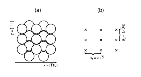
FIG. 1.: (a) A schematic view of the (112) surface of bcc
metals. (b) The corresponding (rectangular) lattice of ad-
sorption sites shown by the crosses ($a=3.16\AA$ for W and
$a=3.14\AA$ for Mo)

.

It turns out, that lattice gas models are quite useful in studying overlayer structures and their properties (e.g. refs [2, 9]). As usual, a lattice gas model introduces the occupation variable $\;n_{\vec{r}}\;$ at each adsorption site $\vec{r}$: $n_{\vec{r}}=1$ if the $\vec{r}$th site is occupied by an adatom and $n_{\vec{r}}=0$, if not. Then, within the grand canonical ensemble, the Hamiltonian is defined as

$${\cal H}=\frac{1}{2}\sum_{\vec{r}\in L}\sum_{\vec{r}^{\prime}\in L\atop\vec{r}^{\prime}\neq\vec{r}}V(\vec{r}-\vec{r}^{\prime})n_{\vec{r}}n_{\vec{r}^{\prime}}-\mu\sum_{\vec{r}\in L}n_{\vec{r}}\;\;\;\;\mbox{,}$$ (1)

where L denotes the rectangular lattice of N$\times$N adsorption sites with periodic boundary conditions and $\mu$ is the chemical potential (shifted, here, by the binding energy of an adatom to the substrate). Of course, $\mu$ controls the adatom coverage

$$\theta=\frac{1}{N^{2}}\sum_{\vec{r}\in L}\langle\>n_{\vec{r}}\>\rangle$$ (2)

with $\langle\>\ldots\>\rangle$ meaning a thermodynamic average. We are interested in a lattice gas model describing linear chain structures as observed experimentally for low coverages ($\theta<0.5$) and, herefore, we can neglect many-body interactions. Since, even in this case, the reliable first-principle calculation of effective lateral interactions is very difficult, following a detailed discussion in ref. [4], we have considered a pairwise adsorbate interaction $V(\vec{r})$ consisting of electrostatic and indirect interactions. Thus, we have assumed

$$V(\vec{r})=\frac{2d^{2}}{|\vec{r}|^{3}}+\left\{\begin{array}[]{lr}A\cos(2k_{F}|y|+\varphi)\frac{1}{|y|}\delta(x,0)&\;{\rm for}\;y\neq 0\\ \\ E_{b}\delta(|x|,a_{1})&\;{\rm for}\;y=0\end{array}\right.\;\;\;\;\mbox{,}$$ (3)

where $\vec{r}=(x,y)$ and $\delta$ stands for Kronecker’s symbol (for notation see also fig. 1). These interactions are of essential importance in forming linear chain structures of alkalis, alkaline-earths, and rare-earths adsorbed on the (112) surface of W or Mo and they have the following meaning:

1. The first component in eq. (3), $\;2d^{2}/|\vec{r}|^{3}\;$, describes a repulsive dipole-dipole interaction between two identical adatoms adsorbed at $\vec{r}$ and $\vec{r^{\prime}}$, respectively (see, for example, refs [4] and [6]). The dipole moment of an adsorption bond, $d$, is usually estimated from the Helmholtz formula. Here, we neglect all depolarization effects due to many-body interactions and this seems to be justified for $\theta<0.5$.

2. The following component for $y\neq 0$, $\;A\cos(2k_{F}|y|+\varphi)\frac{1}{|y|}\delta(x,0)\;$, represents an asymptotic part of the indirect interaction between adatoms via conduction electrons of the substrate (all relevant literature on this interaction could be found in refs [4] and [10]). This particular interaction is highly anisotropic and is closely related to the existence of nearly flattened segments of the Fermi surface being perpendicular to the $[\>\overline{1}\overline{1}1\>]$ axis directed along the atomic troughs of the substrate. An amplitude $A$ and a phase $\varphi$ can be treated as phenomenological parameters and $k_{F}$ denotes a wavevector of electrons at the Fermi surface. In our model we assume, following refs [11, 12], that $k_{F}=0.41\AA^{-1}$ ($k_{F}=0.47\AA^{-1}$) for the tungsten (molybdenum) substrate. It is needless to say, that this indirect (oscillatory) interaction is long-ranged ($\sim|y|^{-1}$) and it could influence, as usually expected, properties of the absorbed submonolayers. We have neglected all contributions to the indirect interaction related to hole segments of the Fermi surface [4, 13].

3. Finally, for $y=0$ the $\;E_{b}\delta(|x|,a_{1})\;$ term has been introduced to eq.(3) to facilitate the formation of linear chains of adatoms along the $x$-direction. This is a part of an attractive indirect interaction between adatoms along a chain and we assume that $E_{b}=-0.05{\rm eV}$ at the nearest-neighbour distance $a_{1}$ [4].

The model interactions, eq. (3), requires, however, some justification.

First, the indirect, substrate mediated interaction (ii) reflects only the leading ”effective” dimensionality of the electronic states (e.g. refs [10],[14]-[15]) mediating the interaction in the direction perpendicular to the chains. Here, we neglect a usual part of the indirect interaction decaying like $\frac{1}{r^{5}}$ and associated with the ”spherical” segments of the Fermi surface [4, 16]. Of course, $r$ denotes a distance between two adatoms.

Secondly, we would like to comment on what role surface electronic states may play in the indirect interaction. It is known, that they could contribute to this interaction provided the Fermi energy level intersects a band of the surface electronic states. Then, depending on the effective dimensionality of the surface states, the indirect interaction becomes proportional either to $\frac{1}{r}$ (quasi–one–dimensional surface states [10], [14]-[15]) or to $\frac{1}{r^{2}}$ (two–dimensional surface states [4], [15]-[16]). A period of the oscillations will be determined by a wavevector at the Fermi surface corresponding to the surface electronic states. Recently, the field and photofield emission experiments on the clean W(112) surface have revealed the existence of surface states approximately 0.3$eV$ below the Fermi energy [17]-[18]. To our knowledge, however, there is so far no experimental evidence that surface states mediate the indirect interaction in the case of the linear chain submonolayers on the (112) surface of W(Mo). Consequently, we have neglected a would be contribution to eq. (3) from the surface states.

Thirdly, the model interaction (iii) could be thought of as a usual substrate mediated interaction in the form $\sim\cos(2k_{F}x+\phi)\delta(y,0)/|x|^{5}$ (see, for example, refs  [16], [19]-[22]). In order to describe the linear chain structures we might assume that $\phi$ causes this indirect interaction to be attractive at the nearest–neighbour distance $a_{1}$ and to decay rapidly with distance. We cannot also exclude a possibility that (iii) might be due to a virtual elastic distortion of the substrate surface [23].

At this stage it is important to notice, that although the interaction described by eq. (3) is long ranged, we may restrict ourselves to an extended but finite range of interaction, $R$. A more detailed discussion will be presented in the following section.

III Properties of the ground states

A search for all the lowest energy configurations at $T=0{\rm K}$ for the model described by eqs (1) and (3) presents a formidable problem. Even in a simpler case of the dipole-dipole interaction only, as far as we know, it has not been possible up to now to find all the ground states. (For a review of the existing theoretical and numerical results concerning the ground states in two-dimensional lattices see, for example, refs [24]-[26] and the literature cited therein.). However, let us note that the ordered phases found experimentally at $T=77{\rm K}$, as we have already discussed, are often composed of parallel linear chains, at least for low coverages ($\theta<0.5$). This suggests, that a search for the minimal grand canonical ensemble energy configurations (the ground states) could be performed in two steps. First, we find the effective Hamiltonian describing interactions between linear chains and only then we look for the ground states.

A The effective Hamiltonian

Making use of the periodicity along the chains, we can write down the Hamiltonian as an effective Hamiltonian of a one-dimensional lattice gas type model, which describes the interaction between linear chains (simply referred to as chains, hereafter). This Hamiltonian has the form

$${\cal H}_{\rm eff}=\frac{1}{2}\sum_{j}\sum_{l(\neq 0)}V(l)\sigma_{j}\sigma_{j+l}-(\mu+\varepsilon_{c})\sum_{j}\sigma_{j}\;\;\;\;\mbox{,}$$ (4)

where $\sigma_{j}$ denotes chain variable with $\sigma_{j}=1$ or 0 depending on whether there is a chain on a site j along the y direction or not. The chain–chain interaction energy at a distance $a_{2}|l|$ reads

$$V(l)=\sum_{k=-\infty}^{+\infty}V_{d}(k,l)+V_{ind}(l)\;\;\;,$$ (5)

where

$\displaystyle V_{d}(k,l)=\frac{2d^{2}}{[k^{2}a_{1}^{2}+l^{2}a_{2}^{2}]^{3/2}}\;\;\;,$

$\displaystyle V_{ind}(l)=A\frac{\cos(2k_{F}a_{2}|l|+\varphi)}{a_{2}|l|}\;\;\;.$

The binding energy per chain can be written as

$$\varepsilon_{c}=-\left(\frac{2d^{2}}{a_{1}^{3}}\>\zeta(3)+E_{b}\right)\;\;\;.$$ (6)

Here, $\zeta(3)=1.202056$…is the Riemann zeta-function and j, l, and k are integers.

It is well known, that the lattice gas effective Hamiltonian, ${\cal H}_{\rm eff}$, is analogous to the Hamiltonian of the Ising model in an applied field. For a class of long-range interactions (positive, convex, etc.) it has been possible to find in a one-dimensional case all the ground states for any rational $0<\frac{q}{p}<1$ ($p$, $q$ are integers with no common multipliers) [26]. Moreover, the $(\theta,\mu)$ phase diagram represents the complete devil’s staircase with a rather involved fractal behaviour [26]-[29]. Unfortunately, the effective Hamiltonian, ${\cal H}_{\rm eff}$, contains the indirect (oscillatory) interaction and, therefore, we are not able to find the ground states rigorously. Also, the results of refs [30, 31] do not seem to be applicable because the considered interaction is truly long-ranged.

B A search for the ground states

As usual, the long-range nature of the effective interaction between chains described by eq. (5) poses a problem. It is easy to see that the interaction is dominated at large distances by the (oscillatory) indirect term and one has to sum up the infinite series (see eq. (4)) for any would-be minimal energy configuration of $\sigma$’s. Instead, we approximate the problem (see also refs [32] and [25]) by assuming that there is a sufficiently large range of the adatom - adatom interaction, say, $R\>a_{2}$, beyond which a configuration under study is replaced by the average one having the same coverage $\theta$. This average chain structure consists of equidistant ”chains” with a spacing $a_{0}=a_{2}/\theta$. Moreover, adatoms are uniformly distributed along these ”chains” with a density $1/a_{1}$.

Finally, we restrict ourselves to periodic configurations of $\sigma$’s, i.e. there is a period $p$ (positive integer) such that $\sigma_{j+p}=\sigma_{j}$ for any integer $j$. These are called $p$-periodic configurations of $\sigma$’s.

Now, the energy per chain of a given $p$-periodic configuration $\sigma_{0},\dots,\sigma_{p-1}$ can be written in the form

$$E[\sigma_{0},\dots,\sigma_{p-1}]=\frac{1}{p}\sum_{j=0}^{p-1}\sum_{l=1}^{R}\tilde{V}(l)\sigma_{j}\sigma_{mod_{p}(j+l)}-\frac{1}{p}(\mu+\varepsilon_{c})\sum_{j=0}^{p-1}\sigma_{j}+E_{r}(\theta)\;\;\;\;\mbox{,}$$ (7)

where

$$\tilde{V}(l)=\sum_{k=-k(l)}^{k(l)}V_{d}(k,l)+V_{\rm ind}(l)$$ (8)

with $k(l)={\rm Int}(\frac{a_{2}}{a_{1}}\sqrt{R^{2}-l^{2}})$.

Here, the remainder of the energy per chain reads

$$E_{r}(\theta) = \theta^{3}\frac{4d^{2}}{a_{1}a_{2}^{2}}\left[\frac{\pi^{2}}{6}-\sum_{n=1}^{{\rm Int}(R\theta)}\frac{\sqrt{1-\left(\frac{n}{R\theta}\right)^{2}}}{n^{2}}\right]+$$ (11)

$$\mbox{}+\theta^{2}\frac{A}{a_{2}}\left[f_{1}(\tilde{\alpha})\cos\varphi+f_{2}(\tilde{\alpha})\sin\varphi+r(\alpha)\right]\;\;\;\;\mbox{,}$$

where

$\displaystyle\theta=\frac{1}{p}\sum_{j=0}^{p-1}\sigma_{j}\;\;\;\;\mbox{,}$

$\displaystyle\alpha=\frac{2k_{F}a_{2}}{\theta}\;\;\;\;\mbox{,}$

$\displaystyle f_{1}(\tilde{\alpha})=-\ln(2\sin\frac{\tilde{\alpha}}{2})\;\;\;\;{\rm for}\;\tilde{\alpha}={\rm mod}_{2\pi}(\alpha)>0\;\;\;\;\mbox{,}$

$\displaystyle f_{2}(\tilde{\alpha})=\frac{\tilde{\alpha}-\pi}{2}\;\;\;\;\;\;\;\;\;{\rm for}\;\tilde{\alpha}={\rm mod}_{2\pi}(\alpha)>0\;\;\;\;\mbox{,}$

$\displaystyle r(\alpha)=\sum_{n=1}^{{\rm Int}(R\theta)}\frac{\cos(n\alpha+\varphi-\pi)}{n}\;\;\;\;\mbox{.}$

The first two components in eq. (7) depend on $\sigma_{0},\dots,\sigma_{p-1}$ and involve exact summations. The remainder of the energy per chain, however, depends only on $\theta$ as it should have been expected. It is interesting to note that this model removes the particle-hole symmetry [2].

In the following, we propose a numerical procedure to find the (periodic) ground states. First, by using the bit representation of integers from the interval $[2^{p-1},2^{p}-1]$ we generate numerically all $p$-periodic configurations of $\sigma$’s with $p=1,\dots,p_{max}$. The number of configurations could then be reduced by making use of the translational and/or inversion symmetries. Secondly, we check explicitly which configurations of $\sigma$’s afford the minimal value to the corresponding $E[\sigma_{0},\ldots,\sigma_{p-1}]$ ($p=1,\ldots,p_{max}$). Of course, the results depend on model parameters, such as $d,A,\varphi,k_{F},R$ and $p_{max}$. This will be discussed in the following subsection.

C The results

To describe a competition between the dipole-dipole and indirect interactions we require three independent parameters: $\;\frac{d^{2}}{A},\varphi$, and $k_{F}$. This results from eq. (7) where $E[\sigma_{0},\ldots,\sigma_{p-1}]$ and $\mu+\epsilon_{c}$ are rescaled by a factor of $A^{-1}$, thus changing effectively only the stability intervals of the ground states but not the ground states themselves. Moreover, our approximation concerning the energy per chain of a given p-periodic configuration of $\sigma^{\prime}s$ (eq. (7)) and the numerical procedure introduce two more parameters: $R$ and $p_{max}$. In principle, calculations should be performed for very large $R$ (the larger the better) and for $\;p_{max}\;$ going to infinity to allow for any periodic structure. In practice, we have carried out calculations for $R=150$ and $p_{max}=23$. This is a compromise between the computing time and more precise results. Our numerical tests show that relative changes of energy at $Ra_{2}=150a_{2}$ (in comparison with $Ra_{2}=1600a_{2}$) are less than one percent for a vast majority of $p$-periodic configurations of $\sigma^{\prime}s$ $(p=1,\ldots,p_{max}=23)$. Also, the results for larger values of $\;p_{max}\;$ change the results only quantatively. We believe, that to understand the role the indirect interaction plays in determining the ground states, no additional significant insight can be achieved by extending the numerical computations to higher values of $\;p_{max}\;$.

We have applied our numerical procedure to determine the ground states for a number of different parameters: $\;\frac{d^{2}}{A},\varphi$, and $k_{F}$. Some of the results are presented in tables I-II and fig. 2. The tables contain sequences of ground states. Here we use standard notation for the ground state, i.e. $q/p$, which means $q$ chains in a unit cell of $p$ sites along the y direction (fig. 1). At the same time $\theta=\frac{q}{p}$ and in the present analysis we are not interested in what are the actual structures of the ground states. Also, it turned out to be convenient to express the strength of the indirect interaction, $A$, in units of $-0.137eV\AA$ (see refs [6] and [16]).

In fig.  2 we have shown explicitly examples of stability intervals of the corresponding ground states with respect to a reduced chemical potential $\mu/\mu_{0}$ ($\mu_{0}=k_{B}T,T=100K$). Note that only halves of the stability intervals for $1/2$ and $2/4$ have been depicted. As usual, the coverage as a function of reduced chemical potential forms the so-called ”staircase”.

Now, we shall discuss the presented results paying a particular emphasis to the role which the indirect interaction plays in determining the ground states.

i) Dependence on $\;\;\frac{d^{2}}{A}$

This parameter is a measure of a competition between the dipole-dipole and indirect interactions. The results shown in table I and fig.2 indicate that by decreasing $\frac{d^{2}}{A}$ (or by increasing the strength of the indirect interaction) one causes the following changes to the ground states:

• For very large values of $\;\frac{d^{2}}{A}\;$ we practically obtain the complete devil’s staircase which is shown in fig. 2(a) (see also refs [26]-[29]).

• For large values of $\;\frac{d^{2}}{A}\;$ many narrow long-periodic ground states (most of which correspond to higher coverages close to $0.5$) disappear from the staircase. The remaining ground states usually change their stability intervals and might transform into the ground states (with a close coverage) (see fig. 2(b)).

• For smaller values of $\;\frac{d^{2}}{A}\;$ the narrow long-periodic ground states (corresponding to low coverages) continue to disappear and we are left with few ground states some of which might be the long periodic ones (see fig. 2(c)). There can even be one ground state (for example, $7/20$ for $d=0.3,A=1$, and other parameters as in fig. 2). This qualitative argument is supported by our calculations for other values of $\varphi$ and $k_{F}$. For example, it also applies to $\varphi=0$ and $\varphi=1.6\pi$ with $k_{F}=0.41\AA^{-1}$ (see table I) but $\;\frac{d^{2}}{A}\;$ must be larger than $2.25$.

At this point we would like to note that in the case of a sufficiently strong indirect interaction for $0.9\pi\leq\varphi\leq 1.5\pi$ and $0.40\AA^{-1}\leq k_{F}\leq 0.50\AA^{-1}$ there is only a coexistence of the low-density ($\theta=0$) and high-density ($\theta=1$) disordered ground states. This means that an attraction effectively prevails between chains, thus leading to formation of two-dimensional islands. This particular result, however, seems not to be accounted for by our model of linear chains (see section III).

ii) Dependence on $\;\;\varphi\;$ and $\;k_{F}$

It is easy to see from tables I-II that the ground states depend on $\varphi$ and $k_{F}$ in a crucial way. The phase, $\varphi$, simply shifts uniformly the locations of minima of the corresponding indirect interaction thus allowing for the ground states with possible new periodicities or$/$and changed stability intervals (in $\mu$). The wavevector, $k_{F}$, distorts uniformly the minima locations and a formation of the ground states is in this case even more complex. Indeed, the results presented in table II indicate that for $\varphi=0$ each sequence of the ground states consists of the ground states having one (two) long-range period(s). Within our model this observation could be understood qualitatively by noting, that for a given $k_{F}$, the actual ground state $q/p$ wins the energy competition between two terms: $E[\sigma_{0},\ldots,\sigma_{p-1}]-E_{r}(\theta)$ involving a structure of a would-be ground state (i.e. $\sigma_{0},\ldots,\sigma_{p-1}$) and $E_{r}(\theta)$, where $\theta=\frac{1}{p}\sum_{j=0}^{p-1}{\sigma_{j}}$ is such that $\tilde{\alpha}$ is close to $0$ or $2\pi$ (see eqs (7), (8), and (11)). This argument seems to be valid also for $\varphi\in(0,\frac{\pi}{2}]$ and $\varphi\in[\frac{3\pi}{2},2\pi)$ despite the fact that the ground states start to gain on their energies. And this gain for $\varphi\in(\frac{\pi}{2},\frac{3\pi}{2})$ is even more dramatic for now there are several new ground states. Apart from long-periodic ground states there are also such ones as, for example, $1/2,\;1/3\;$, and $\;1/4$ (see table I).

IV Phase diagrams. Mean-field treatment

As a first step we adopt the mean-field approximation (a discussion concerning the validity of this approach is postponed until the following section) to describe (equilibrium) phase diagrams for linear chains structures with the competing dipole-dipole and long-range indirect (oscillatory) interactions. In the following, we restrict ourselves to the effective Hamiltonian ${\cal H}_{eff}$, eqs (4), (5), and (6) with a finite range of the adatom - adatom interaction $R_{eff}$. The reason is that thermal fluctuactions ”screen out” the long-range indirect interaction [4] and it is plausible to assume for a qualitative analysis, at least, that $R_{eff}$ does not depend on temperature and the dipole-dipole interaction can be neglected for distances larger than $R_{eff}a_{2}$.

Following the standard procedure (e.g. ref. [2]) we can write the mean-field Hamiltonian in the form

$${\cal H}_{eff}^{MF}=\sum_{i}{(V_{i}-\tilde{\mu})\sigma_{i}}-\frac{1}{2}\sum_{i}{V_{i}\langle\sigma_{i}\rangle}\;\;\;\;\mbox{,}$$ (12)

where

$$V_{i}=\sum_{j}{\tilde{V}(i-j)\langle\sigma_{j}\rangle}\;\;\;\;\mbox{,}$$ (13)

and

$$\langle\sigma_{i}\rangle=\left[1+e^{\beta(V_{i}-\tilde{\mu})}\right]^{-1}\;.$$ (14)

Again, $\sigma_{j}$ denotes the chain variable with $\sigma_{j}=0$ or $1$. Moreover, $\tilde{V}(i-j)$ is given by eq. (8) with $R$ replaced by $R_{eff}$ and $\tilde{\mu}=\mu+\epsilon_{c}$ with $\epsilon_{c}$ defined via eq. (6).

First, we solve the self-consistent eqs (13) and (14). This becomes possible to do, if we assume, that the resulting structure is a $p$-periodic one, $p=1,\ldots,p_{max}$. Usually the solution will not be unique (i.e. several ordered structures are possible). Secondly, having found the solution(s) we can calculate the corresponding grand canonical ensemble potential(s) per chain

$$\Omega(T,\tilde{\mu})=-\frac{1}{p}\sum_{i=0}^{p-1}{\left\{ln\left[1+e^{-\beta(V_{i}-\tilde{\mu})}\right]+\frac{1}{2}V_{i}\langle\sigma_{i}\rangle\right\}}\;\;\;.$$ (15)

Hence, the stable structure corresponds to the minimal value of $\Omega(T,\tilde{\mu})$, while the other structures are metastable or unstable ones.

In the computations we assume $R_{eff}=36$ (i.e. $R_{eff}a_{2}\approx 100\AA$) and $p_{max}=12$ according to the ”lever rule” between a computing time and more refined phase diagrams. It seems that $p_{max}=12$ is sufficient to account for some linear chain structures determined by the LEED technique [4].

A Dipole-dipole interaction

We start with a model of linear chain structures which order via the dipole-dipole interaction only (with an additional attraction along the chains). This model might be relevant to adsorption on furrowed surfaces, where the indirect interaction can be neglected (small $A$ or lack of the corresponding flattened segments of the Fermi surface of a substrate).

The results of the calculations are presented in fig. 3. This is a temperature ($T$) versus reduced chemical potential ($\frac{\mu}{\mu_{0}},\mu_{0}=k_{B}T,T=100K$) phase diagram, where we have denoted equilibrium (stable) phases by their ground states notation $q/p$. Note, that there is one exception to the rule, i.e. the higher-temperature case, $4/10$, which has no the ground state equivalent. The phase diagram is shown for $\mu>-0.72\mu_{0}$ and this is due to our restriction to $p_{max}=12$. The most interesting result is the following: the thermal fluctuations suppress long periodic phases and most of the phase diagram is dominated by the phases $1/2$, $1/3$, and $1/4$. This occurs despite the long-range nature of the dipole-dipole interaction. (Note that a similar observation was reported in ref. [33] for a two-dimensional model with short-range interactions).

B Application to Li/W(112) and Li/Mo(112)

We claim that our model of linear chain structures might qualitatively account for the adsorption of lithium atoms on the $(112)$ surfaces of W and Mo [4], [34]-[35]. The adsorption bonds are polarized and at a low coverage, $d=1.7D$ and $d=1.4D$ for the W and Mo substrates, respectively. Also, we expect the indirect interaction to be important (see section II). Finally, no ”hard core” effects (a relatively small atomic radius of a lithium atom) make the model more realistic.

We have found two sets of the model parameters which might be relevant to Li/Mo(112) and Li/W(112) and the quantative features of the corresponding mean-field phase diagrams are summarized in figs 4 and 5. Both these figures have some common features. That is, the horizontal hatching indicates coexistence regions between ordered (equilibrium) phases denoted as in fig. 3. These are the so-called ”mixed-phases” regions. A dashed curve represents a second order phase transition curve between the low density $(\theta=0)$ lattice gas phase and $1/2$ phase. This curve meets, at some angle, two tangent first order phase transition curves at a multicritical point P.

Now, a direct comparison of the phase transition schemes for Li/Mo(112) [34] and for Li/W(112) [35] with a low temperature vs coverage sequence of transitions of fig. 4 and fig. 5, respectively, shows a qualitative similarity.

In fig. 4, a low temperature scheme of phase transition corresponds quite well to Li/Mo(112) because the first order transitions occur through forming islands of a phase in the ”mixed-phase” region. It is also interesting to note a high thermal stability of $1/4$ and $1/2$ phases at the corresponding stoichiometries.

The phase diagram presented in fig. 5, however, needs some more explanation. The cross-hatching depictes a region where the results do not seem to be reliable due to our restriction to $p_{max}=12$. We have also found that at low temperatures and close to the disordered phase ($\theta<0.05$) our numerical iteration procedure of solving eqs (13) and (14) turns out to be non-convergent (oscillatory behaviour). Therefore, we consider only ($\theta>0.05$). Even so, we recover (not too close to the disorder phase) a low temperature sequence of $1/4$, $1/3$, and $1/2$ phases. Of course, the present theory cannot describe the phase transition between $1/4$ and $1/3$ phases occuring via a kind of statistical mixture of phases (cf. [36, 37]). Let us note that below $\sim 80K$ there are long-periodic structures (i.e. $1/6$ and $1/9$). Thus, providing thermal fluctations do not destroy the long-range order, we expect that these phases could be observed experimentally below $77K$. We are aware of the approximations we have made so far and, therefore, no more direct comparisons are going to be made. A discussion of the validity of this approach to the other linear chain structures will be presented in the following section.

V Discussion and conclusions

The main results obtained in this paper fall into two categories, i.e.

1. Ground states analysis of the effective energy, eqs (7), (8), and (11) concerning the role of the long-range indirect interaction. The results were obtained numerically and this was done without any approximations. We have shown that the interaction modifies in an essential way the ground states as obtained from the dipole-dipole interaction only. The general tendency is such that by increasing an amplitude of the indirect interaction, $A$, one reduces the number of ground states. The full description, however, requires other parameters of the interaction, i.e. $k_{F}$ and $\varphi$. A detailed discussion is presented in section III C.

2. Temperature versus coverage (or $T$ vs $\mu$) phase diagrams based on the effective Hamiltonian ${\cal H}_{eff}$, eqs (4), (5), and (6), and computed numerically within the molecular-field approximation.

It seems that (ii) needs more discussion. It is well known that the mean–field treatment does not account for (thermal) fluctuations correctly especially in low dimensional systems [1, 26]. As a consequence, the long-range order might be destroyed and a topology of phase diagrams and/or the order of various transitions are not often correct. This has been discussed and demonstrated explicitly for short-range interactions by comparing mean-field results with the corresponding Monte Carlo simulations, real-space or finite-size renormalization group (cf. [38, 39]).

In our opinion, it would be very interesting to study the problem of fluctuations in the case of long-range (also oscillatory) interactions in ”2.5Dimensional” systems [25, 40]. In this context, our mean-field results can be treated as zeroth-order approximation.

The role of the indirect interaction has a great impact on the phase diagrams despite the fact that it is quite weak ($\frac{A}{a_{2}}\sim 0.05eV$). Numerical computations show in an explicit way that this interaction is responsible for causing longer periodic phases to develop high thermal stability. Figs 3-5 illustrate this situation. The above conjecture, although based on the mean-field theory, is corroborated by the recent Monte Carlo simulation [19]. Note, however, that the indirect interaction used in ref. [19] is characterized by only three parameters and has no-oscillatory behaviour.

We think, it is a challange to extend (if practically possible) Monte Carlo simulation or other more ”exact” methods to long-range (oscillatory) interactions, which seems to be important in adsorption at crystal surfaces. Also, it would be very interesting to determine experimentally the whole ($T,\theta$) phase diagrams to check theoretical predictions.

The present work was concerned with adsorption of lithium atoms on furrowed surfaces of Mo and W . However, other alkaline (alkaline-earth or rare-earth) atoms are larger in diameter and, therefore, our theory will have to be modified for ”hard-core” effects. A kind of modification is also needed to account for more complex structures.

This paper has dealt with the indirect interaction decaying like $\frac{1}{r}$ which is closely related to both the face and form of the Fermi surface of the substrate (W and Mo). In general, however, the indirect interaction has an asymptotic form $\sim cos(2k_{F}r+\varphi)/r^{\beta}$, with $\beta\in[1,5]$ [4].

We would like to end with the following comment. It is now well known that the precise power law behaviour of this interaction might depend upon the form of the Fermi surface, surface electronic states, virtual elastic distortion of the substrate surface, etc. Therefore, it would be very interesting to study a competition between the dipole–dipole and indirect ($\beta>1$) interactions in view of possible physical applications. This problem turns out to be quite difficult for it requires a novel numerical method of convergence of series and the results will be published elsewhere.

Acknowledgements

The authors are indebted to Professor Jan Kołaczkiewicz for discussions and a critical reading of the manuscript. Several comments from the referee have been useful. Two of us (J.L and Cz.O) kindly acknowledge a financial support from the State Committee for Scientific Research (KBN) via the grant No. 2 P302 113 05. A part of the numerical computations was performed at the Supercomputing Centre in Poznań, Poland.

FIG. 2.: Coverage as a function of reduced chemical potential, $\frac{\mu}{\mu_{0}}$ ($\mu_{0}=k_{B}T,T=100K$), for $\varphi=1.2\pi,k_{F}=0.41\AA^{-1}$ and $a=3.16\AA$. (a) The devil’s staircase: $d=1.5$ and $A=0$. (b) The devil’s-like staircase: $d=1.5$ and $A=1$. (c) The ”normal” staircase: $d=0.5$ and $A=1$. Here $d$ and $A$ are expressed in units of Debye and $-0.137eV\AA$, respectively. For a detailed discussion see the text.

FIG. 3.: Mean-field phase diagram: T versus $\frac{\mu}{\mu_{0}}$ ($\mu_{0}=k_{B}T,T=100K$). Here $d=1.5D$, $E_{b}=-0.05eV$, $a=3.14\AA$. b and c denote the corresponding insets. For a notation see the text.

FIG. 4.: Mean-field phase diagram (T versus $\theta$ ) for $d=1D$, $A=-0.274eV\AA$, $k_{F}=0.47\AA^{-1}$, $\varphi=0.93\pi$, $E_{b}=-0.05eV$ and $a=3.14\AA$. For an explanation cf. text.

FIG. 5.: Mean-field phase diagram (T versus $\theta$) for $d=1.5D$, $A=-0.137eV\AA$, $k_{F}=0.41\AA^{-1}$, $\varphi=1.26\pi$, $E_{b}=-0.05eV$ and $a=3.16\AA$. For an explanation cf. text.

TABLE I.: Sequences of the ground states as a function of phase, $\varphi$. Here, $k_{F}=0.41\AA^{-1}$ ($a=3.16\AA$) and $k_{F}=0.47\AA^{-1}$ ($a=3.14\AA$) are considered because of a possible application to Li/W(112) and Li/Mo(112). ($\;\frac{d^{2}}{A}\;$ is expressed in units of $-7.299D^{2}eV^{-1}\AA^{-1}$).

	$d^{2}/A=2.25$
	$k_{F}=0.41{\AA}^{-1}$					$k_{F}=0.47{\AA}^{-1}$
$\varphi/\pi$	0.0	0.4	0.8	1.2	1.6	0.0	0.4	0.8	1.2	1.6
	5/14	1/11	2/23	1/15	5/14	4/22	4/22	1/14	1/13	1/5
		2/11	1/10	1/12		5/22	5/22	2/23	3/22	5/20
		3/11	3/18	2/21		6/22	6/22	3/22	1/6	4/15
		4/11	4/23	1/9		7/22	7/22	2/11	3/15	1/3
		1/2	1/5	2/15		8/22	8/22	4/19	3/11	2/5
			1/4	2/13		9/22	9/22	1/4	1/3
			8/23	4/21		10/22	1/2	9/22	9/22
			9/23	2/10		11/22		1/2	1/2
			3/7	1/4
			1/2	2/7
				1/3
				1/2
	$d^{2}/A=0.25$
	5/14	4/11	8/22	7/20	5/14	8/22	8/22	9/22	9/22	1/5
		1/2	1/2	2/4		10/22	10/22	1/2		2/5
						11/22	11/22

TABLE II.: Sequences of the ground states as a function of wavevector, $k_{F}$, for $\varphi=0$ and $a=3.16\AA$. For a discussion see the text. ($\;\frac{d^{2}}{A}\;$ is expressed in units of $-7.299D^{2}eV^{-1}\AA^{-1}$).

	$d^{2}/A=2.25$
$k_{F}$	0.40	0.41	0.42	0.43	0.44	0.45	0.46	0.47	0.48	0.49
	7/23	5/14	3/11	2/8	3/13	5/23	1/5	4/22	2/12	1/7
	8/23		7/22	3/8	4/13	6/23	2/5	5/22	3/12	2/7
	9/23		4/11	4/8	5/13	7/23		9/22	4/12	8/21
	10/23		9/22		6/13	8/23			5/12	3/7
	11/23		5/11			9/23			6/12	10/21
			1/2			10/23
						11/23
	$d^{2}/A=0.25$
	8/23	5/14	3/11	3/8	4/13	8/23	2/5	9/22	4/12	2/7
	9/23		7/22	4/8	6/13	9/23			6/12	8/21
	10/23		9/22			10/23				10/21
	11/23		5/11			11/23

REFERENCES

- [1] A.G. Naumovets, Surf. Sci. 299/300 (1994) 706 and references cited therein.
- [2] B.N.J. Persson, Surf. Sci. Rep. 15 (1992) 1.
- [3] A. Zangwill, Physics at Surfaces. (Cambridge University Press, Cambridge, 1988).
- [4] O.M. Braun and V.K. Medvedev, Soviet Phys. Usp. 32 (1989) 328 and references cited therein.
- [5] L.A. Bolshov, A.P. Napartovich, A.G. Naumovets and A.G. Fedorus, Soviet Phys. Usp. 20 (1977) 432.
- [6] T.T. Tsong, Rep. Prog. Phys. 51 (1988) 759.
- [7] V.K. Medvedev and A.I. Yakivczuk, Fiz. Tverd. Tela 20 (1975) 1900.
- [8] V.K. Medvedev and A.I. Yakivczuk, Fiz. Tverd. Tela 21 (1979) 313.
- [9] W. Selke, K. Binder and W. Kinzel, Surf. Sci. 125 (1983) 74.
- [10] B. Gumhalter and W. Brenig, Prog. Surf. Sci. 48 (1995) 39.
- [11] R.F. Girvan, A.V. Gold and R.A. Phillips, J. Phys. Chem. Solids 29 (1968) 1485.
- [12] V.V. Boiko and V.A. Gasparov, Zh. Eksp. Teor. Fiz. 61 (1971) 2362.
- [13] O.M. Braun, Fiz. Tverd. Tela 22 (1980) 2079.
- [14] B. Gumhalter and W. Brenig, Surf. Sci. 336 (1995) 326.
- [15] E. Bertel, Surf. Sci. 331–333 (1995) 1136.
- [16] K.H. Lau and W. Kohn, Surf. Sci. 75 (1978) 69.
- [17] D. Venus and M.J.G. Lee, Surf. Sci. 172 (1986) 477.
- [18] T. Radoń and S. Jaskółka, Surf. Sci. 247 (1991)106.
- [19] I.N. Yakovkin, Surf. Sci. 282 (1993) 195.
- [20] F. Flores, N.H. March and I.D. Moore, Surf. Sci. 69 (1977) 133.
- [21] K. Joyce, A. Martin-Rodero, F. Flores, P.J. Grout and N.H. March, J. Phys. C: Solid State Phys. 20 (1987) 3381.
- [22] N.H. March, Phys. Rev. B 39 (1989) 1385.
- [23] W. Kappus, Z. Phys. B 29 (1978) 239.
- [24] M. Kaburagi and J. Kanamori, J. Phys. Soc. Japan 43 (1977) 1686.
- [25] L.D. Roelofs and Donna L. Kriebel, J. Phys. C: Solid State Phys. 20 (1987) 2937.
- [26] I. Lyuksyutov, A.G. Naumovets and V. Pokrovsky, Two-Dimensional Crystals (Academic Press, Boston, MA, 1992).
- [27] P. Bak and R. Bruinsma, Phys. Rev. Lett. 49 (1982) 249.
- [28] S. Aubry, J. Phys. Lett. (Paris) 44 (1983) L247.
- [29] R. Bruinsma and P. Bak, Phys. Rev. B 27 (1983) 5824.
- [30] T. Morita, J. Phys. A: Math., Nucl. Gen. 7 (1974) 289.
- [31] T. Morita, J. Phys. A: Math., Nucl. Gen. 7 (1974) 1613.
- [32] V.K. Medvedev and I.N. Yakovkin, Sov. Phys. Solid State 19 (1977) 1515.
- [33] K. Binder and D.P. Landau, Phys. Rev. B21 (1980) 1941.
- [34] M.C. Gupalo, V.K. Medvedev, B.M. Palyuh and T.P. Smereka, Fiz. Tverd. Tela 21 (1979) 973.
- [35] V.K. Medvedev , A.G. Naumovets and T.P. Smereka, Surf. Sci. 34 (1973) 368.
- [36] P. J. Estrup and J. Anderson, Surf. Sci. 8 (1967) 101.
- [37] R. L. Gerlach and T. N. Rhodin, Surf. Sci. 17 (1969) 32.
- [38] K. Binder, W. Kinzel and D.P. Landau, Surf. Sci. 117 (1982) 232 and refernces therein.
- [39] K. Binder and D.P. Landau, Surf. Sci. 61 (1976) 577.
- [40] J.M. Moison, Cond. Matt. News 2 (1993) 17.