Scalable Parallel Numerical Methods
and Software Tools for Material Design

Abstract

A new method of solution to the local spin density approximation to the electronic Schrödinger equation is presented. The method is based on an efficient, parallel, adaptive multigrid eigenvalue solver. It is shown that adaptivity is both necessary and sufficient to accurately solve the eigenvalue problem near the singularities at the atomic centers. While preliminary, these results suggest that direct real space methods may provide a much needed method for efficiently computing the forces in complex materials.

1 Introduction

To intelligently design materials with specific high performance properties, it is necessary to have an understanding of the underlying atomic structure, reactive sites, and other properties of complex candidate compounds. To achieve the generality and reliability needed to predict these properties, methods based on the first principles solution to the electronic Schrödinger equation are required. For systems of typical size, the most reliable and efficient first principles approach is based on the local density approximation (LDA) of Kohn and Sham [8] to the full many-electron Schrödinger equation. However, current methods of solution scale as $O(N^{3})$, where $N$ is the number of atoms. For systems of the size commonly encountered in materials science, such calculations are too large to be practical.

The goal of our program is to develop methods that can efficiently treat large and complex systems. To be successful, we must solve the following computational issues:

• The method must be fast to allow simulations requiring thousands of atomic interaction evaluations.

• The method must be capable of high accuracy: .02 eV/atom.

• The method must effectively capture the multiple length scales inherent in the problem.

• The method must scale as $N^{2}$ or less to allow extension to larger systems.

To address these goals, we are developing the following techniques and software tools:

• A rapidly converging method for the non-linear eigenvalue problem arising in the LDA.

• Adaptive methods for resolving the locality of electronic wavefunctions with multiple length scales.

• A software infrastructure to exploit the high performance parallel architectures capable of providing the throughput and memory we require.

2 The LDA Equations

In the LDA, the electronic wavefunctions are given by the solutions to the eigenvalue problem:

(1) $${\cal H}\psi_{i}=\lambda_{i}\psi_{i}$$

where the Hamiltonian ${\cal H}$ is given by:

(2) $${\cal H}=\left(\frac{-\nabla^{2}}{2m}+V_{ext}+V_{H}+V_{xc}\right)$$

$\lambda_{i}$ is an eigenvalue, and the eigenvectors (the wavefunctions $\psi_{i}$) satisfy the usual orthonormality constraints of a symmetric operator. In general, we require the lowest $N$ eigenvalues, where $N$ is the number of electrons in the system. Electron-electron interaction is included in the Hartree potential, $V_{H}$, and the exchange correlation potential, $V_{xc}$. Both $V_{H}$ and $V_{ex}$ are functions of the charge density $\rho(\vec{x})=\sum_{occ}\psi_{i}^{2}$, where the sum includes only occupied orbitals. $V_{H}$ is the solution to Poisson’s equation in free space with this charge density.

Since $V_{H}$ and $V_{xc}$ are functionals of the electron density, Eq. (1) must be solved self-consistently. That is, an initial density is input and iterations continue until the input and output densities are the same. The $V_{ext}$ potential term represents the attractive interactions of the electrons to the atomic nuclei and is a function of the positions of the atoms. In our simulations, Eq. (1) must be solved many times as the position of the atoms change.

There are several length scales in the solution of Eq. (1). The overall dimension of the system is determined by the atomic positions and the associated electron density. However, each atomic center is associated with a length related to the effective charge of its nucleus. For example, sodium has a small atomic charge and, therefore, a fairly long length scale ($\approx 2.5$ Å). On the other hand, oxygen has a high effective charge and a corresponding very short length scale ($\approx.5$ Å).

The presence of several length scales in Eq. (1) poses significant difficulties for present solution methods, based on the FFT. Since increases in the overall dimension of the system and the resolution of the function in real space (because of a short length scale) both require increases in the size of the basis, the use of a planewave basis requires the retention of a very large numbers of basis functions. The computational cost of this is somewhat offset by the high parallelism and efficient vectorization of the algorithm. However, because of the steepness of the atomic potentials, we have found that on the order of $10^{4}$ to $10^{6}$ Fourier functions may be required to obtain sufficient accuracy. Such calculations are extremely CPU intensive.

The eigenvalue equation for a real system is complicated by details which obscure the essential difficulties of its solution [9]. To develop test problems (see Section 4) which retain the essential singular behavior while removing nonessential details, we replace $V_{H}$, $V_{ext}$, and $V_{ex}$ by simple potentials located at the atomic sites. The solution to these eigenvalue problems provide little information as to the convergence properties of the numerical method with respect to self-consistency or the efficiency of the solution to the embedded Poisson problem. However, they enable us to address the critical issues of multiple length scales and the singular behavior of the potential.

3 Parallel Adaptive Solution to the Eigenvalue Problem

We have developed a parallel adaptive eigenvalue solver (AMG) which integrates adaptive mesh refinement techniques [3] [2] with a novel multigrid eigenvalue algorithm [4]. To our knowledge, this is the first time such methods have been combined to solve materials science problems.

We solve the eigenvalue problem using the multigrid method of Cai et al. [4]. Given the linear eigenvalue problem ${\cal H}\psi=\lambda\psi$, the following efficiently calculates the lowest eigenvalue and eigenvector:

	let $\psi$ be an initial guess ($\psi\neq 0$)
	repeat
		${\cal H}$-normalize $\psi$: $(\psi,{\cal H}\psi)=1$
		let $\lambda=(\psi,{\cal H}\psi)/(\psi,\psi)$
		perform one multigrid V-cycle on $({\cal H}-\lambda I)\psi=0$
	until $\|({\cal H}-\lambda I)\psi\|<\varepsilon$ (some error tolerance)

Convergence is rapid; for a typical problem, machine precision is reached within fifteen iterations. As with most iterative methods, a good initial guess can significantly speed convergence. To calculate eigenvalues other than the lowest, we apply the above procedure and, after each V-cycle, orthogonalize the candidate eigenvector against all previously calculated eigenvectors.

Because of the multiple length scales present in our problems, we cannot efficiently represent the eigenvector $\psi$ using a uniform discretization of space. Uniform grids cannot adapt in response to local changes; thus, the grid spacing is dictated by the shortest length scale present in the entire problem. Instead, we represent $\psi$ as a composite grid (see Figure 1), which enables our solver to locally refine the discretization as required by local phenomena. By exploiting locality, we expend computational resources (flops and memory) in those regions of the solution where they are most needed.

Figure 1: Wavefunctions are resolved on a composite grid which represents a non-uniform discretization. In practice, composite grids are implemented as a hierarchy of grid levels.

A composite grid logically consists of a single grid in which the discretization is non-uniform. Such grids are actually represented using a hierarchy of levels (see Figure 1). All grids at the same level have the same mesh spacing, but successive levels have finer spacing than the ones preceding it, providing a more accurate representation of the solution. We locally refine the grid hierarchy according to an error estimate calculated at run-time. In general, the location and extent of refinement areas must be computed by the application, as they cannot be predicted a priori.

We implemented our solver using the LPARX [6] parallel programming system, which provides efficient run-time support for scientific calculations with dynamic, block structured data. The use of LPARX was essential in facilitating code development; managing the complicated data structures of a composite grid hierarchy would have been a daunting task without LPARX, especially on parallel architectures. LPARX enables us to run the same code on a diversity of high performance parallel architectures, including the CM-5, Paragon, single processor workstations, Cray C-90, SP-1, and networks of workstations. For more details concerning the implementation and performance, refer to [7] in these proceedings.

4 Model Problems

All of the following model problems were solved in 3d; we did not attempt to exploit symmetry. Each AMG solution required approximately one minute running on an IBM RS/6000 model 590.

4.1 The Hydrogen Atom

In this problem, the Hamiltonian has a deceptively simple form with only a single term:

(3) $${\cal H}=-\frac{\nabla^{2}}{2m}-\frac{Z}{r}.$$

While the eigenvalue problem corresponding to Eq. (3) can be solved analytically, the singular behavior at $r=0$ can cause significant problems for numerical methods. In fact, it cannot be conveniently solved with our present FFT methods. For example, for the lowest eigenvalue, our FFT algorithm with $64^{3}$ mesh points gives the value -0.69 rather than the correct value of -0.5. The lowest energy solution in our units is an exponential with the form $e^{-Zr}$ and energy $E=\frac{Z^{2}}{2}$. Note that the severity of the singularity with increasing $Z$ is reflected in the increasing localization of the solution around the origin. As $Z$ increases, the density of points in an adaptive method will increase near the origin.

The $Z=1$ solution corresponds to the hydrogen problem. It is plotted in Figure 2(a). We note that the AMG solution and the exact solution (not plotted) are identical on the scale of the graph. The cusp at the origin is a result of the singular nature of the potential at this point. This behavior is usually difficult to resolve with a numerical method [5].

As the singularity strengthens with increasing charge, the lowest energy scales as $Z^{2}$. Figure 2(b) illustrates how this behavior is reproduced by the AMG solution. As expected, to obtain the correct scaling, it is necessary to go to higher levels of adaptivity. However, because of increased localization, the total number of points remains roughly the same. To illustrate the efficiency of adaptivity, we note that the resolution at the finest level is equivalent to a uniform grid with $4096^{3}$ basis elements, as compared to the fewer than $64^{3}$ points required by the adaptive algorithm.

   

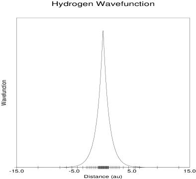
Figure 2: The left graph displays the lowest energy eigenvector for the hydrogen atom; graph data was extracted from the 3d volume along the $Z$ axis. Tick marks on the abscissa represent mesh points. The right plot shows the eigenvalues for a $\frac{-Z}{R}$ potential.

4.2 The $\mbox{H}_{2}^{+}$ Molecule

A problem that is similar to the hydrogen atom problem, but more commonly used as a test problem for chemical methods, is the $\mbox{H}_{2}^{+}$ molecule. In this problem, there is only one electron. However, there are two centers with singularities. The Hamiltonian is:

(4) $${\cal H}=\frac{-\nabla^{2}}{2m}-\frac{1}{|\vec{r}+\frac{\vec{R_{a}}}{2}|}-\frac{1}{|\vec{r}-\frac{\vec{R_{a}}}{2}|},\mbox{where $\vec{R_{a}}$ is the atomic separation.}$$

This problem can also be solved analytically [1]. Again, it is two stiff for practical solution by FFT. On the other hand, the AMG method does quite well as illustrated by the binding energy curve in Figure 3(b). (Binding energy is defined as the total energy of the atoms at a specified distance minus the energy at infinite separation.) The wave function is plotted in Figure 3(a). Note the increased density of points in the vicinity of the nuclei.

   

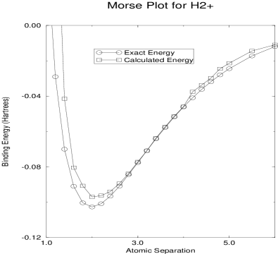
Figure 3: The left graph displays the lowest energy eigenvector for the hydrogen molecular ion; graph data was extracted from the 3d volume along the $Z$ axis. Tick marks on the abscissa represent mesh points. The right plot shows binding energy as a function of atomic separation.

4.3 Adaptive Multigrid vs. FFT

In this test problem, we soften the singularities in the original potential by introducing an error function with a variable cut off ($r_{\rm cut}$). We replace the $\frac{1}{r}$ potentials of Eq. ( 4) with the smoothed potentials $erf(\frac{r}{r_{\rm cut}})/r$. If this potential is sufficiently softened (i.e. $r_{\rm cut}$ is large), the FFT, the uniform grid, and the AMG methods will all converge to the same answer. Results are summarized in Table 1. The exact answer for these parameters and $r_{\rm cut}=0$ is -0.911. It is clear that both the uniform grid method and the FFT method lose accuracy quickly as $r_{\rm cut}$ approaches 0.

Table 1: A comparison of eigenvalues for the FFT, adaptive multigrid solver, and a uniform grid solver. All methods used approximately the same number of basis elements. The known solution for $r_{\rm cut}=0$ is -0.911.

$r_{\rm cut}$	FFT	Adaptive	Uniform
0.0	-1.0946	-0.9005	-1.2009
0.1	-0.9986	-0.8931	-1.0353
0.2	-0.8998	-0.8734	-0.9035
0.3	-0.8664	-0.8551	-0.8672
0.4	-0.8427	-0.8325	-0.8430

References

- [1] D. R. Bates, K. Ledsham, and A. L. Stewart, Wave functions of the hydrogen molecular ion, Phil. Trans. Roy. Soc. London, 246 (1953), pp. 215–240.
- [2] M. J. Berger and P. Colella, Local adaptive mesh refinement for shock hydrodynamics, Journal of Computational Physics, 82 (1989), pp. 64–84.
- [3] M. J. Berger and J. Oliger, Adaptive mesh refinement for hyperbolic partial differential equations, Journal of Computational Physics, 53 (1984), pp. 484–512.
- [4] Z. Cai, J. Mandel, and S. McCormick, Multigrid methods for nearly singular linear equations and eigenvalue problems. (submitted for publication), 1994.
- [5] K. Cho, T. A. Arias, J. D. Joannopoulos, and P. K. Lam, Wavelets in electronic structure calculations, Physical Review Letters, 71 (1993), pp. 1808–1811.
- [6] S. R. Kohn and S. B. Baden, A robust parallel programming model for dynamic non-uniform scientific computations, in Proceedings of the 1994 Scalable High Performance Computing Conference, May 1994.
- [7] , The parallelization of an adaptive multigrid eigenvalue solver with LPARX, in Proceedings of the Sixth SIAM Conference on Parallel Processing for Scientific Computing, San Francisco, CA, Februrary 1995.
- [8] W. Kohn and L. Sham, Phys, Rev., 140 (1965), p. A1133.
- [9] M. W. Sung, Molecular Dynamics Simulation Of Metallic Clusters and Heteroclusters, PhD thesis, University of California, San Diego, 1994.