Reciprocal Space Analysis of Short Range Order Intensities by the Cluster Variation Method

Abstract

A reciprocal space formulation of the Cluster Variation is used in order to extract effective pair interactions in alloys from experimental short-range order diffuse intensities. The method is applied to the analysis of the short range order contribution to the neutron diffuse scattering of a $Fe-19.5{\%}Al$ single crystal. A detailed comparison with real space methods is carried out for three different levels of approximations. For the highest level of approximation used in this study, effective pair interactions up to fifth neighbors are obtained.

I Introduction

The diffuse scattering of X-rays and neutrons remains the technique of choice for quantitative studies of short-range order (SRO) in alloys. In particular, the part of the diffuse intensity related to substitutional SRO has played a prominent role in alloy theory. This SRO intensity contains important information on the effective interactions between atoms which, in turn, can be used to characterize thermodynamic properties of the alloy, such as relative phase stability, phase diagrams and antiphase boundary energies.

Experimental measurements of SRO intensity have evolved significantly from the studies in polycrystalline materials of the early 1950’s. At present, accurate measurements are carried out in single crystals at high and low temperature. For example, recent work has focused on the use of high flux neutron and tunable synchrotron X-ray sources. [1, 2, 3, 4, 5, 6, 7] On the theoretical side, the study of SRO intensity in alloys and its characterization through diffuse scattering dates back to the pioneering work of Cowley, [8] Krivoglaz [9] and Clapp and Moss. [10, 11] Out of these studies emerged what is presently known as the Krivoglaz-Clapp-Moss (KCM) formula. This formula establishes a simple relationship between the experimentally observed diffuse scattering and the Fourier transform of the effective pair interactions. The KCM formula corresponds to a treatment of concentration fluctuations at the lowest level of approximation for the alloy configurational free energy, namely the single site mean-field approximation, also known as the Bragg-Williams [12] and the molecular field approximation.

More recently, effective pair interactions have been obtained from experimentally determined SRO intensities using higher approximations based on Monte Carlo simulations and the Cluster Variation Method (CVM). [13] The first calculation of SRO intensity carried out directly in reciprocal space using the cluster variation method was done by Sanchez in 1982. [14] This k-space formulation of the CVM provides a significant improvement over the KCM formula, although a price is paid in increased computational effort. Thus, despite the improved treatment of fluctuations by the CVM, the method has been applied only to very few cases. [14, 15] An alternative approach, which we will refer to as the real space inverse CVM was introduced by Gratias and Cénédèse. [16] In this method, the effective pair interactions are obtained by fitting a few Warren-Cowley SRO parameters which, in turn, are related by a Fourier transform to the experimentally determined SRO intensity. A definite advantage of the real space inverse CVM is that the method involves only a modest computational effort, comparable to that of a regular CVM equilibrium calculation. On the other hand, the main drawback of the real space technique is that the fitting is done for only a few Warren-Cowley SRO parameters which, typically, are not enough to describe the measured intensities. To a great extent, this problem is solved by applying the inverse method in real space using Monte Carlo simulations, in which longer interaction ranges may be included without any fundamental difficulties. [17, 18] A problem of a slightly different nature is the fact that the determination of the Warren-Cowley SRO parameters from the experimental intensities, despite the fact that they are uniquely defined in terms of a Fourier transform, is not without errors. This step in the procedure, which of necessity requires the introduction of a real space cut-off in SRO, is an additional source of uncertainty on the derived effective pair interactions.

Here we proposed a new method that carries out the fitting of the SRO intensity directly in k-space using the CVM formulation of the SRO intensity of Sanchez. [14] Since the Warren-Cowley SRO parameters are not required, the k-space fitting circumvents two of the main problems of the real space method, namely the cut-off in SRO and the determination of the SRO parameters which, as mentioned, must be obtained by either fitting or by Fourier transformation of the experimental data. The method is applied to diffuse neutron scattering data obtained at several temperatures for a $Fe-19.5at{\%}Al$ single crystal.[6] A comparison between the real and k-space methods is also carried out for three different approximations of the CVM.

The organization of the paper is as follows. In Section II we describe briefly the experimental aspects. The theoretical model and a review of the CVM formulation of the SRO intensity is given in Section III. Results are presented in Section IV with concluding remarks given in Section V.

II Experimental Considerations

The experimental results, including standard corrections to the data, have been reported in previous publications.[4, 6] Thus, here we briefly recall only the main experimental aspects, referring the reader to Refs. [[4, 6]] for further details.

The diffuse scattering measurements were carried out at high temperatures on D7 at ILL (Grenoble, France), using a 10 mm in diameter and 20 mm long cylindrical single crystal of $Fe-19.5at{\%}Al$ oriented along the [110] direction. Time of flight analysis was used in order to eliminate the phonon and critical magnetic contributions. Here we analyze four temperatures between $1273K$ and $1573K$. The cross sections were calculated using the classical corrections (instrumental background, double scattering and absorption). The experimental points were averaged with a weight inversely proportional to the square of their error to obtain a regular grid of points (mesh of 0.1 reciprocal lattice unit step).

In order to obtain the SRO intensity, the experimentally determined neutron scattering cross section was corrected for contributions due to static and dynamic atomic displacements. The correction for static displacements was carried out using the method based on the formulation of Borie and Sparks, [20] whereas dynamic attenuation was treated using the standard Debye-Waller theory. It should be noted that the accuracy of these corrections affect critically the reliability of the effective interactions derived from the diffuse intensity.

In terms of the experimental scattering cross section, the corrected intensity in Laue units is written:

$${I_{corr}(\vec{k})}={1\over{NF_{Laue}}}\left[\displaystyle{{d\sigma}\over{d\Omega}}(\vec{k})\enskip e^{(Bk^{2}/8\pi^{2})}-I_{inc}\right]$$ (1)

where $N$ the total number of atoms and $F_{Laue}$ is the usual normalization factor given by $F_{Laue}=c(1-c)(b_{Al}-b_{Fe})^{2}$, with $c$ the aluminum concentration, and $b_{Al}$ and $b_{Fe}$ the nuclear diffusion lengths of $Al$ and $Fe$, respectively. In Eqn. (1), $I_{inc}$ is the incoherent scattering and $B$ the Debye-Waller factor.

Following Borie and Sparks, [20] the corrected intensity is approximated by a first order expansion in the atomic displacements $\vec{u}_{\bf p}$, where the subindex ${\bf p}$ stands for the set of integers $(p_{1},p_{2},p_{3})$ and the location of lattice site ${\bf p}$ is given by $\vec{R}_{\bf p}={\displaystyle{a\over 2}}(p_{1},p_{2},p_{3})$. In this approximation, the corrected intensity at the reciprocal space vector $\vec{k}=\displaystyle{{2\pi}\over a}(h_{1},h_{2},h_{3})$ can be written as:

$$I_{corr}(\vec{k})=\alpha(\vec{k})\enskip+\enskip\sum_{i=1}^{3}h_{i}Q_{i}(\vec{k})$$ (2)

where $\alpha(\vec{k})$ is the SRO contribution we are interested in, and the $Q_{i}(\vec{k})$ are related to the Fourier transform of the atomic displacements. We next consider each of these two terms separately.

The SRO intensity $\alpha(\vec{k})$ is given by the Fourier transform of the Warren-Cowley SRO parameters $\alpha_{\bf p}$:

$$\alpha(\vec{k})=\sum_{\bf p}\enskip\alpha_{\bf p}\enskip cos(\vec{k}\cdot\vec{R}_{\bf p})$$ (3)

with $\alpha_{\bf p}$ defined by:

$$\alpha_{\bf p}={{<\sigma_{\bf o}\sigma_{\bf p}>-<\sigma_{\bf o}>^{2}}\over{1-<\sigma_{\bf o}>^{2}}}$$ (4)

where $\sigma_{\bf o}$ and $\sigma_{\bf p}$ are occupation numbers at the origin and at site $\bf p$, respectively. These occupation numbers take values $1$ or $-1$ if the lattice site is occupied by $Fe$ or $Al$ atoms, respectively, and the brackets $<>$ stand for configurational averages.

The quantities $\vec{Q}(\vec{k})=[Q_{1},Q_{2},Q_{3}]$ in Eqn. (2) are given by the first order displacement parameters $\vec{\gamma}_{\bf p}$:

$$\vec{Q}(\vec{k})=\sum_{\bf p}\enskip\vec{\gamma}_{\bf p}\enskip sin(\vec{k}\cdot\vec{R}_{\bf p})$$ (5)

In turn, the displacement parameters $\vec{\gamma}_{\bf p}$ are defined by:

$$\vec{\gamma}_{\bf p}=-{{2\pi}\over a}\enskip\sum_{\sigma=\pm 1}\sum_{\sigma^{\prime}=\pm 1}\enskip{b_{\sigma}b_{\sigma^{\prime}}\over F_{Laue}}\enskip\rho_{2,{\bf p}}(\sigma\sigma^{\prime})\enskip<\Delta\vec{u}_{\bf p}^{\sigma\sigma^{\prime}}>$$ (6)

where $<\Delta\vec{u}_{\bf p}^{\sigma\sigma^{\prime}}>$ is the average relative displacement between atoms of type $\sigma$ and $\sigma^{\prime}$ (i.e. $Fe$ or $Al$) separated by $\vec{R}_{\bf p}$, and where $\rho_{2,{\bf p}}(\sigma\sigma^{\prime})$ is the probability of finding atoms $\sigma$ and $\sigma^{\prime}$ separated by distance $\vec{R}_{\bf p}$. We note that these probabilities are $c^{2}+c(1-c)\alpha_{\bf p}$, $(1-c)^{2}+c(1-c)\alpha_{\bf p}$ and $c(1-c)-c(1-c)\alpha_{\bf p}$ for $AlAl$, $FeFe$ and $FeAl$ pairs, respectively.

The quantities $\alpha(\vec{k})$ and $\vec{Q}(\vec{k})$ are invariant to any symmetry operation of the space group of the reciprocal lattice, whereas the diffuse intensity $I_{corr}(\vec{k})$ is not. Consequently, the experimental points can be grouped into families of equivalent k-points having the same values of $\alpha(\vec{k})$ and $\vec{Q}(\vec{k})$, but with different intensities $I_{corr}(\vec{k})$. Families having as many or more k-points than unknowns ($\alpha(\vec{k})$ and $\vec{Q}(\vec{k})$) can be used to separate both contributions from $I_{corr}(\vec{k})$.

Since for the (110) reciprocal plane $Q_{1}=Q_{2}$, there are at most 3 unknowns on this plane. We note that at special points the number of unknowns is further reduced by symmetry to either 2, when $Q_{1}=Q_{2}=Q_{3}$, or 1, when $Q_{1}=Q_{2}=Q_{3}=0$. The maximum number of independent measurements possible at some of the equivalent points is 6. However, the measurement range in reciprocal space is limited by the neutron wavelength and by the lack of accuracy in the diffuse scattering around the Bragg peaks due to the mosaic structure of the single crystal and to different parasitic contributions. These limitations reduce strongly the occurrence of 6 equivalent measurement points. In fact, in the more frequent case there are 4 experimental points for three unknowns. In such cases (24 measured points), the unknowns were solved using a weighted least square fit, with a weight inversely proportional to the square of the experimental error. Thus, for each such point in the first Brillouin zone, one obtains a value $\alpha(\vec{k})$ with an error bar, $\Delta\alpha(\vec{k})$, and a measure of the quality of the fit, $\chi^{2}$, given by the weighted sum of the square of the difference between the measured and fitted values. In order to take into account the quality of the fit, the error bar $\Delta\alpha(\vec{k})$ was multiplied by $\chi$ when the latter was larger than one. For 18 k-points, the number of unknowns is equal to the number of experimental points. In these cases the system was solved and the error bar was multiplied by the maximum $\chi$ of the first class of points. Finally, for ten points, mainly located around the origin and at the edges of the measured region, there are less measurements than unknowns and, therefore, it is not possible to separate $\alpha(\vec{k})$ and $\vec{Q}(\vec{k})$ from the measured intensity.

A point of clarification concerning the Debye-Waller factors is also in order. These were measured from the attenuation of the fundamental Bragg peaks through neutron and gamma ray scattering. [19] We note, however, that the attenuation of the Bragg peaks is related to the sum of the dynamic, $B_{d}(T)$, and static, $B_{s}$, Debye-Waller factors, i.e. $B_{lro}=B_{d}(T)+B_{s}$, whereas the attenuation of the short range order intensity is given by their difference, $B=B_{d}(T)-B_{s}$. In order to separate these two contributions, the static part was assumed to be temperature independent. Since this approximation results in large errors in $B_{d}(T)$ at high temperature, the restriction of a temperature independent static Debye-Waller factor was subsequently lifted by including a correction $\Delta B(T)$ in the SRO attenuation: [19]

$$B=B_{d}(T)-B_{s}+\Delta B(T)$$ (7)

The correction $\Delta B(T)$ was determined by exploiting the symmetry of the corrected intensity as well as using a least square fit of the experimental data at equivalent k-points. The latter procedure was carried using points for which the number of unknowns is smaller than the number of measurements.

The values of $\Delta B(T)$ obtained by the two different methods are very similar at high temperatures, indicating that the Borie and Sparks model is adequate to describe the scattering cross section. Departure are seen at low temperatures, likely due to the magnetic short range order contributions which are not explicitly considered in the analysis. Thus, the high temperature data reported in Refs.[[6]] are considered to be the most accurate, and we will consequently restrict the present analysis to them.

Figure 1 shows the experimental SRO intensity at $1273K$ after all corrections have been made, together with the fit obtained with 8 Warren-Cowley SRO parameters (solid line). In what follows, we will refer to these quantities as the experimental Warren-Cowley SRO parameters, although they are actually the result of fitting the $\alpha(k)$. In the fit, a value $\alpha_{0}=1.147$ was obtained, which is to be compared with the exact value of 1. Each integer step on the horizontal axis of Fig. 1 corresponds to a scan along the $(00h_{3})$ direction, with $h_{3}$ between 0 and 1, for fixed values of $h_{1}=h_{2}$. We note that the SRO data at the other temperatures analyzed here, namely $1373K$, $1473K$ and $1573K$, look qualitatively the same. Furthermore, at these temperatures, a similar quality of the fit is also achieved with 8 shells of $\alpha_{n}$’s.

A notable feature of the SRO intensity is the small peak observed near the origin. It is not clear from the experimental data, however, whether this maximum is real or it is simply an artifact due to the cut-off imposed on the SRO parameters and/or to the fact that the fitting was carried out on only one plane in reciprocal space. The presence of this maximum, whether real or not, poses interesting questions on the use of the real space inversion methods. We will return to this point after discussing the theoretical models used to describe the SRO intensity in alloys.

III Theory

In this section we develop a simple statistical model in order to calculate the observed SRO diffuse intensity in terms of the effective pair interactions. We begin by describing the Hamiltonian, which is to be solved at finite temperatures using different levels of approximation of the CVM, continue with a brief description of the approach used to calculate the SRO intensity, and conclude with a description of the inverse methods employed to determine the pair interactions.

A The Hamiltonian

We describe the $Fe-Al$ system with a simple Ising model in which the magnetic moments are localized on the $Fe$ atoms:

$$H_{0}=-\frac{1}{8}\enskip\sum_{{\bf p},{\bf p^{\prime}}}\enskip J_{\bf pp^{\prime}}\enskip(1+\sigma_{\bf p})(1+\sigma_{\bf p^{\prime}})\enskip S_{\bf p}S_{\bf p^{\prime}}$$ (8)

$$+\frac{1}{2}\enskip\sum_{{\bf p},{\bf p^{\prime}}}\enskip V_{\bf pp^{\prime}}^{c}\enskip\sigma_{\bf p}\sigma_{\bf p^{\prime}}$$ (9)

where $S_{\bf p}=\pm 1$ is the spin at site $\bf p$. In Eqn. (9), $V_{\bf pp^{\prime}}^{c}$ and $J_{\bf pp^{\prime}}$ are, respectively, effective chemical and exchange interactions between sites $\bf p$ and $\bf p^{\prime}$. Averaging over the magnetic degrees of freedom, the interacting part of the alloy Hamiltonian can be written as:

$$H_{2}=\frac{1}{2}\enskip\sum_{{\bf p},{\bf p^{\prime}}}\enskip\tilde{V}_{\bf pp^{\prime}}\enskip\sigma_{\bf p}\sigma_{\bf p^{\prime}}$$ (10)

where the effective pair interaction is:

$$\tilde{V}_{\bf pp^{\prime}}=V_{\bf pp^{\prime}}^{c}\enskip-\enskip\frac{1}{4}J_{\bf pp^{\prime}}<S_{\bf p}S_{\bf p^{\prime}}>$$ (11)

We note that in terms of interatomic potentials between different chemical species, the effective interactions are given by:

$$\tilde{V}_{\bf pp^{\prime}}=\frac{1}{4}\enskip[\tilde{V}_{\bf pp^{\prime}}^{FeFe}+\tilde{V}_{\bf pp^{\prime}}^{AlAl}-2\enskip\tilde{V}_{\bf pp^{\prime}}^{FeAl}]$$ (12)

Thus, in the present model, the unknown magnetic SRO is included in the effective pair interactions, which now should depend on temperature. [4] Furthermore, since the product $J_{\bf pp^{\prime}}<S_{\bf p}S_{\bf p^{\prime}}>$ in Eqn. (11) is alway positive, the $\tilde{V}_{\bf pp^{\prime}}$ are smaller than the chemical interactions $V_{\bf pp^{\prime}}^{c}$.

B Cluster Variation Method

The Hamiltonian in Eqn. (10) is solved at finite temperatures using the Cluster Variation Method. In this approximation, the alloy free energy is written in terms of the probabilities of finding different atomic configurations on clusters of lattice sites. A given cluster, consisting of $n$ lattice points (${\bf p}_{1},{\bf p}_{2},...,{\bf p}_{n}$), will be characterized by a set of indices $\bf n$, describing the geometry and the orientation of the cluster, and by its location in the lattice, $\vec{r}_{\bf n}$. As needed, the three features of the cluster, type and orientation $\bf n$ and location $\vec{r}_{\bf p}$, will be collectively denoted by $\beta=[{\bf n},\vec{r}_{\bf p}]$. Here we adopt the convention that the location of the cluster is given by its the center of gravity:

$$r_{\bf n}={1\over n}\enskip\sum_{{\bf p}\in\beta}\enskip\vec{R}_{{\bf p}}$$ (13)

For a given cluster $\beta=[{\bf n},\vec{r}_{\bf n}]$ there are $2^{n}$ atomic configurations, each one described by the set of occupation numbers $\vec{\sigma}_{\beta}=[\sigma_{{\bf p}_{1}},...\sigma_{{\bf p}_{n}}]$. The probability of occurrence of any one of these configurations will be called $\rho_{\beta}(\vec{\sigma}_{\beta})$.

With the energy given by Eqn. (10), the CVM free energy functional takes the form: [21]

$${\cal F}=\frac{1}{2}\enskip\sum_{{\bf p},{\bf p^{\prime}}}\enskip\tilde{V}_{\bf pp^{\prime}}\enskip<\sigma_{\bf p}\sigma_{\bf p^{\prime}}>+\sum_{\bf p}\mu_{\bf p}<\sigma_{\bf p}>$$ (14)

$$-k_{B}T\enskip\sum_{\beta}\enskip a_{\beta}\enskip\sum_{\vec{\sigma}_{\beta}}\enskip\rho_{\beta}(\vec{\sigma}_{\beta})\enskip ln\left(\rho_{\beta}(\vec{\sigma}_{\beta})\right)$$ (15)

where we have included a staggered effective chemical potential field $\mu_{\bf p}$, which will be used in the next subsection to describe general concentration fluctuations. The coefficients $a_{\beta}$ in Eqn. (15) are central to the CVM. After choosing a set of maximum clusters $\{\gamma\}$, which determines the level of approximation, the coefficients $a_{\beta}$ are calculated from the following recursive relations: [21]

$${\sum_{\alpha\supseteq\beta}}^{{}^{\prime}}a_{\alpha}=1$$ (16)

where the sum is restricted to clusters $\alpha$ contained in the set of maximum clusters $\gamma$, i.e. for clusters $\alpha\subseteq\{\gamma\}$. Furthermore, Eqn. (16) is valid for all clusters $\beta$ included in the approximation, i.e. $\beta\subseteq\{\gamma\}$. The coefficients $a_{\beta}$ have the full symmetry of the disordered lattice and, therefore, they are independent of the location and orientation of the cluster. Furthermore, these coefficients are uniquely defined once the set of maximum clusters is chosen.

The free energy functional, Eqn. (15), must be minimized with respect to the cluster probabilities $\rho_{\beta}(\vec{\sigma}_{\beta})$ subject to normalization constraints:

$$\sum_{\vec{\sigma}_{\alpha}}\enskip\rho_{\alpha}(\vec{\sigma}_{\alpha})=1$$ (17)

and, for all clusters $\beta\subseteq\alpha$, subject to the self consistency requirement:

$$\rho_{\beta}(\vec{\sigma}_{\beta})={\sum_{\vec{\sigma}_{\alpha}}}^{{}^{\prime}}\enskip\rho_{\alpha}(\vec{\sigma}_{\alpha})$$ (18)

where the sum is carried out over the occupation numbers $\sigma_{\bf p}=\pm 1$ for all lattice sites p contained in $\alpha$ but outside cluster $\beta$.

A general description of the cluster probabilities, in which Eqns. (17) and (18) are strictly obeyed, can be achieved by using a complete and orthogonal basis set of characteristic functions. [21, 22] These functions, in turn, can be used to describe any function of configuration, of which the probabilities $\rho_{\beta}(\vec{\sigma}_{\beta})$ are a particular case. For binary systems, the characteristic functions, which we will denote ${\mathchoice{{\hbox{\boldmath$\displaystyle\sigma$}}}{{\hbox{\boldmath$\textstyle\sigma$}}}{{\hbox{\boldmath$\scriptstyle\sigma$}}}{{\hbox{\boldmath$\scriptscriptstyle\sigma$}}}}_{\beta}$, are defined for each cluster $\beta$ in the lattice by the product of the occupation numbers $\sigma_{\bf p}$ over all points $\bf p$ contained in $\beta$:[21]

$${\mathchoice{{\hbox{\boldmath$\displaystyle\sigma$}}}{{\hbox{\boldmath$\textstyle\sigma$}}}{{\hbox{\boldmath$\scriptstyle\sigma$}}}{{\hbox{\boldmath$\scriptscriptstyle\sigma$}}}}_{\beta}=\prod_{{\bf p}\in\beta}\enskip\sigma_{\bf p}$$ (19)

In this basis, the cluster probabilities take a particularly simple form:[21]

$$\rho_{\beta}(\vec{\sigma}_{\beta})={1\over{2^{n}}}\enskip\left[1+\sum_{\alpha\subseteq\beta}{\mathchoice{{\hbox{\boldmath$\displaystyle\sigma$}}}{{\hbox{\boldmath$\textstyle\sigma$}}}{{\hbox{\boldmath$\scriptstyle\sigma$}}}{{\hbox{\boldmath$\scriptscriptstyle\sigma$}}}}_{\alpha}<{\mathchoice{{\hbox{\boldmath$\displaystyle\sigma$}}}{{\hbox{\boldmath$\textstyle\sigma$}}}{{\hbox{\boldmath$\scriptstyle\sigma$}}}{{\hbox{\boldmath$\scriptscriptstyle\sigma$}}}}_{\alpha}>\right]$$ (20)

where the multisite correlations, $<{\mathchoice{{\hbox{\boldmath$\displaystyle\sigma$}}}{{\hbox{\boldmath$\textstyle\sigma$}}}{{\hbox{\boldmath$\scriptstyle\sigma$}}}{{\hbox{\boldmath$\scriptscriptstyle\sigma$}}}}_{\alpha}>$, given by the expectation value of the characteristic functions, form a set of linearly independent configurational variables. These multisite correlation can be conveniently used in the free energy minimization:

$${\partial{\cal F}\over\partial<{\mathchoice{{\hbox{\boldmath$\displaystyle\sigma$}}}{{\hbox{\boldmath$\textstyle\sigma$}}}{{\hbox{\boldmath$\scriptstyle\sigma$}}}{{\hbox{\boldmath$\scriptscriptstyle\sigma$}}}}_{\beta}>}=0$$ (21)

The minimum of $\cal F$ defines the equilibrium free energy, $F$, as well as the equilibrium values of the multisite correlation functions, $<{\mathchoice{{\hbox{\boldmath$\displaystyle\sigma$}}}{{\hbox{\boldmath$\textstyle\sigma$}}}{{\hbox{\boldmath$\scriptstyle\sigma$}}}{{\hbox{\boldmath$\scriptscriptstyle\sigma$}}}}_{\beta}>$. The latter, of course, have the symmetry of the equilibrium phase. In the usual case in which the effective chemical potential field is spatially uniform, the number of correlation functions $<{\mathchoice{{\hbox{\boldmath$\displaystyle\sigma$}}}{{\hbox{\boldmath$\textstyle\sigma$}}}{{\hbox{\boldmath$\scriptstyle\sigma$}}}{{\hbox{\boldmath$\scriptscriptstyle\sigma$}}}}_{\beta}>$ is relatively small. In such cases, the set of Eqns. (21) can be solved efficiently using fast numerical algorithms based, for example, in the Newton-Raphson method. In the next subsection, we will study the response of the system to small arbitrary variations in the effective chemical potential. The analysis leads to the fluctuation spectrum of the concentration variable $<\sigma_{\bf p}>$, which is directly related to the observed SRO intensity.

C Fluctuations

We note that solution of Eqns. (21) yields a set of correlations or, equivalently, Warren-Cowley SRO parameters for only those pairs included in the set of maximum clusters $\{\gamma\}$. Typically, the Warren-Cowley parameters obtained in this manner are not sufficient to reproduce the experimental SRO intensity. Thus, the required long-range pair correlations are calculated using a different approach, based on the fluctuation spectrum obtained with the CVM free energy, Eqn. (15). For the sake of completeness, we summarize here the main results needed for the calculation of SRO intensities using the CVM, and refer the reader to the original work for further details. [14] Following Ref. [[14]], we write the pair correlations as:

$$<\sigma_{\bf p}\sigma_{{\bf p}^{\prime}}>-<\sigma_{\bf p}><\sigma_{{\bf p}^{\prime}}>=-k_{B}T{\partial^{2}F\over{\partial\mu_{\bf p}\partial\mu_{{\bf p}^{\prime}}}}$$ (22)

A Fourier transform of Eqn. (22) yields: [14]

$$<|\sigma(\vec{k})|^{2}>-|<\sigma(\vec{k})>|^{2}=-k_{B}T{\partial^{2}F\over{\partial\mu(\vec{k})\partial\mu(-\vec{k})}}$$ (23)

with:

$$\sigma(\vec{k})=\sum_{\bf p}\enskip\sigma_{\bf p}\enskip e^{-i\vec{k}\cdot\vec{R}_{\bf p}}$$ (24)

and

$${\partial\over\partial\mu(\vec{k})}=\sum_{\bf p}\enskip e^{-i\vec{k}\cdot\vec{R}_{\bf p}}{\partial\over\partial\mu_{\bf p}}$$ (25)

Actual calculation of the right hand side of Eqn. (23) requires the Fourier transform of the matrix of second derivatives of the free energy with respect to the correlation functions:

$$F_{{\bf n},{\bf n^{\prime}}}(\vec{k})={1\over N}\enskip\sum_{\vec{r}_{\bf n},\vec{r}_{\bf n^{\prime}}}\enskip F_{{\bf n},{\bf n^{\prime}}}(\vec{r}_{\bf n}-\vec{r}_{\bf n^{\prime}})\enskip e^{-i\vec{k}\cdot(\vec{r}_{\bf n}-\vec{r}_{\bf n^{\prime}})}$$ (26)

where the sum is over all the locations $\vec{r}_{\bf n}$ and $\vec{r}_{\bf n^{\prime}}$ in the lattice of clusters of type $\bf n$ and $\bf n^{\prime}$ and where $F_{{\bf n},{\bf n^{\prime}}}(\vec{r}_{\bf n}-\vec{r}_{\bf n^{\prime}})$ is given by:

$$F_{{\bf n},{\bf n^{\prime}}}(\vec{r}_{\bf n}-\vec{r}_{\bf n^{\prime}})={\partial^{2}{\cal F}\over{\partial<{\mathchoice{{\hbox{\boldmath$\displaystyle\sigma$}}}{{\hbox{\boldmath$\textstyle\sigma$}}}{{\hbox{\boldmath$\scriptstyle\sigma$}}}{{\hbox{\boldmath$\scriptscriptstyle\sigma$}}}}_{\beta}>\partial<{\mathchoice{{\hbox{\boldmath$\displaystyle\sigma$}}}{{\hbox{\boldmath$\textstyle\sigma$}}}{{\hbox{\boldmath$\scriptstyle\sigma$}}}{{\hbox{\boldmath$\scriptscriptstyle\sigma$}}}}_{\beta^{\prime}}>}}$$ (27)

with $\beta=[{\bf n},\vec{r}_{\bf n}]$ and $\beta^{\prime}=[{\bf n^{\prime}},\vec{r}_{\bf n^{\prime}}]$.

Since the effective chemical potential $\mu(\vec{k})$ is the conjugate thermodynamic variable of the point correlation function $<\sigma(\vec{k})>$, the second derivatives in Eqn. (23) are given by: [14]

$$-{\partial^{2}F\over{\partial\mu(\vec{k})\partial\mu(-\vec{k})}}=NF_{1,1}^{-1}(\vec{k})$$ (28)

where $F_{1,1}^{-1}(\vec{k})$ is the diagonal element corresponding to the point correlation function (${\bf n}={\bf n^{\prime}}=1$) of the inverse of the matrix $F_{{\bf n},{\bf n^{\prime}}}(\vec{k})$.

Combining Eqns. (4), (23) an (28), we obtain the desired result to be used in the fitting of the SRO intensity:

$$\alpha(\vec{k})={Nk_{B}TF_{1,1}^{-1}(\vec{k})\over{1-<\sigma_{\bf o}>^{2}}}$$ (29)

The procedure leading to Eqn. (29) is equivalent to expanding the free energy around equilibrium up to second order in the correlation functions, and describing the fluctuation spectrum in the Gaussian approximation. As mentioned, Eqn. (29) yields a significantly improved description of the SRO intensity over the Krivoglaz-Clapp-Moss formula. We note that although accuracy is generally gained as the cluster size increases, the size of the matrix of second derivatives $F_{{\bf n},{\bf n^{\prime}}}(\vec{k})$ can rapidly grow beyond practical limits. In the next section, we will describe results for a CVM approximation that include clusters of up to nine points, which yields a complex second derivative matrix of size $1088\times 1088$.

D Inverse k-Space Method

The simplest procedure to obtain effective pair interactions from the measured SRO intensity consists in calculating the Warren-Cowley SRO parameters $\alpha_{\bf p}$ from the measured $\alpha(\vec{k})$, and then proceed to solve for the interactions using Eqns. (21) with the proper constraints on the pair probabilities. As mentioned, this real space inverse method has been applied to several cases using both the CVM and Monte Carlo simulations. Here we propose an alternative approach that does not require the computation of the real space Warren-Cowley SRO parameters but, instead, obtains the pair interactions by fitting $\alpha(\vec{k})$, calculated using Eqn. (29), to those obtained experimentally. The procedure consists in minimizing the following sum of errors squared:

$$\chi^{2}={1\over M}\enskip\sum_{i=1}^{M}\enskip\left[{{\alpha_{m}(\vec{k}_{i})-\alpha_{c}(\vec{k}_{i})}\over{\Delta\alpha(\vec{k}_{i})}}\right]^{2}$$ (30)

with $M$ the number of measurements, $\alpha_{m}(\vec{k}_{i})$ and $\alpha_{c}(\vec{k}_{i})$ the measured and calculated SRO intensities, respectively, and where $\Delta\alpha(\vec{k}_{i})$ is the experimental errors determined as described in Section II.

In order to estimate the errors in the effective interactions $\tilde{V}_{n}$ obtained from the least square fitting, we consider the probability distribution for the SRO intensity to be of the form:

$$P(\{\alpha(\vec{k})\})\propto\prod_{i=1}^{M}\enskip exp\left[-{\delta\alpha(\vec{k}_{i})^{2}\over\Delta{\alpha(\vec{k}_{i})}^{2}}\right]$$ (31)

with $\delta\alpha(\vec{k}_{i})=\alpha(\vec{k}_{i})-<\alpha(\vec{k}_{i})>$.

The corresponding probability distribution for the effective interactions, up to second order in $\tilde{V}_{n}$, is then given by:

$$P(\{{\tilde{V}}_{n}\})\propto\prod_{n}\enskip exp\left[-{\sum_{m,n}A_{m,n}{\delta{\tilde{V}}_{m}\over\Delta{\tilde{V}}_{m}}{\delta{\tilde{V}}_{n}\over\Delta{\tilde{V}}_{n}}}\right]$$ (32)

with $\delta{\tilde{V}}_{m}={\tilde{V}}_{m}-<{\tilde{V}}_{m}>$ and $A_{m,n}$ given by:

$$A_{n,m}=\sum_{i=1}^{M}\enskip{1\over{\Delta\alpha(\vec{k}_{i})}^{2}}\enskip{\partial\alpha(\vec{k}_{i})\over\partial{\tilde{V}}_{n}}{\partial\alpha(\vec{k}_{i})\over\partial{\tilde{V}}_{m}}$$ (33)

Thus, an estimate of the error in the effective interactions can be obtained from the eigenvalues, $\lambda_{n}$, and the matrix of eigenvectors, $\vec{\nu}_{n,m}$, of $A_{m,n}$:

$$\Delta{\tilde{V}}_{n}=\chi\enskip\sum_{m}\enskip{|\nu_{n,m}|\over\sqrt{\lambda_{n}}}$$ (34)

where we have included the factor $\chi$, which is typically larger than one, in order to take into account the quality of the fit in the error of the effective interactions.

IV Results

The methods described in the previous section were applied to the three different approximations of the CVM, which will be referred to as the tetrahedron (T), the cube-octahedron (C-O) and the cube-rhombohedron-octahedron (C-R-O) approximations. The maximum cluster for each of these approximations are shown in Fig. 2. In the T approximation, only first and second neighbors are involved. The C-O approximation, which has been used previously in the context of the real space inverse CVM, [4, 6] extends the range up to fifth neighbors. In this approximation, however, the fourth neighbor pairs are excluded since they do not belong to the maximum clusters (the body-centered-cube and the octahedron). This difficulty is resolved by the C-R-O approximation since the additional rhombohedron cluster includes fifth neighbor pairs.

A Real Space Method

First, we apply the standard inverse CVM. For comparison purposes we have carried out the calculations in all three approximation, although the T approximation is not expected to be very reliable in this case since only two Warren-Cowley parameters are used in the fit. The results are shown in Table I where the first column lists the Warren-Cowley SRO parameters extracted from the experimental data for the first 5 neighbor shells. We recall that 8 shells of $\alpha_{i}$’s have been used in the experimental analysis of the data. [4, 6] We also note that in the C-R-O approximation all the $\alpha_{i}$’s listed in Table I are reproduced exactly, whereas in the C-O approximation there is no information on $\alpha_{4}$ and in the T approximation only the first 2 $\alpha_{i}$’s are reproduced.

The values of ${\tilde{V}}_{n}$ are comparable in the three approximations, with the notable exception of ${\tilde{V}}_{2}$ that is three to four times smaller in the C-R-O than in the other two approximations. A direct test of the quality of the inverse CVM results can be obtained by calculating $\alpha(\vec{k})$, as described in Section III.C, using the interactions of Table I. The results of these calculations for the three approximation are compared to the experimental data in Fig. 3.

Overall, the quality of the fit for all three approximations is not very satisfactory. The T approximation (dotted line in Fig. 3), with only two effective interactions, gives a very poor agreement near the maximum at $(0.5,0.5,0.5)$. On the other hand, the C-O approximation (dashed line in Fig. 3) reproduces this maximum quite well, although it fails to reproduce the increase in intensity predicted by the experimental $\alpha_{n}$’s (see Fig. 1). As mentioned, the poor fit near the origin may not be particularly important since, based on the k-space data, the existence of a maximum near the origin is questionable. Nevertheless, this failure of the C-O approximation to reproduce the diffuse intensity maximum illustrates two problematic aspects of the real space inverse CVM: i) The fact that the cut-off in SRO may introduce spurious effects in the SRO intensity and, ii) The fact that fitting just a few of the Warren-Cowley SRO parameters is not enough to reproduce all the features of the SRO intensity.

The inverse CVM in the C-R-O approximation (full line in Fig. 3) works very well around $(0.5,0.5,0.5)$, reproduces the diffuse intensity maximum near the origin, but it gives poor agreement around (001).

Finally, in order to illustrate the problems that may arise from using the C-O approximations, in which fourth neighbor pairs are not considered (i.e. ${\tilde{V}}_{4}=0$), we have calculated the Warren-Cowley SRO parameters using the C-R-O approximation with the interactions obtained in the C-O approximation. The results are shown in the last column of Table I. We see that the $\alpha_{4}$ predicted by the interactions of the C-O approximation differs in sign from the experimental one, given in the second column in Table I.

B Reciprocal Space Method

The difficulties encountered in the application of the inverse CVM to the $Fe-Al$ data are likely due to the uncertainty and errors in the experimental determination of the $\alpha_{n}$’s. Although this difficulty can in principle be resolved by measuring more points on several reciprocal space planes, a more elegant solution is to fit the SRO intensity directly in k-space. The resulting pair interactions at $1273K$, together with the predicted $\alpha_{n}$’s, are shown in Table II. We see from the table that the interactions, particularly for the nearest- and next-nearest-neighbor pairs, are significantly different from those obtained using the real space method. Another noticeable difference is that the interactions shown in Table II change very little as we go from one approximation to the next. In Figure 4 we show a comparison between the results of the real space (open symbols) and reciprocal space (full symbols) methods for the T (triangle), C-O (circles) and C-R-O (squares) approximations. The lines connecting the ${\tilde{V}}_{n}$’s obtained in the C-R-O approximation are drawn as an aid to the eye only.

The SRO intensity corresponding to the interactions of Table II are shown in Fig. 5. We see that the overall fit has improved considerably relative to that obtained with the real space method. Furthermore, the three approximations give essentially the same intensity. This is understood from the fact that the dominant interactions are the first and second neighbors (see Table II). Thus, the T approximation is already sufficient to capture the main features of the diffuse intensity. The increase in intensity near the origin predicted by the experimental $\alpha_{n}$’s is not present in any of the three approximations.

Since the dominant effective interactions are between first and second neighbors, the SRO intensity for the other temperatures investigated here were analyzed using the T approximation. The results for ${\tilde{V}}_{1}$ and ${\tilde{V}}_{2}$ as a function of temperature are shown in Fig. 6. There is a gradual increase in the effective interactions with temperature which is expected from the decrease in magnetic SRO (see Eqn. (11)).

V Conclusions

The determination of effective interactions from measured SRO intensities requires considerable manipulation of the experimental data. In this process, the guidance of reliable theoretical models is invaluable. In particular, we have shown that the ability to calculate accurately the diffuse intensity in reciprocal space allows the determination of the effective interactions without the intermediate step of obtaining the Warren-Cowley SRO parameters in real space. Consequently, the method proposed here avoids the need to introduce a real space cut-off in SRO.

The study of fluctuations in reciprocal space by means of the CVM allows the description of statistical correlations beyond the range of effective interactions. This establishes a fundamental difference with the KCM formula, derived from the Bragg-Williams approximation, in which the fluctuation spectrum is determined entirely by the Fourier transform of the interaction potentials. Furthermore, these statistical correlations, which extend beyond the range of the effective interactions, are describe well using relatively small clusters. For example, for the $Fe-Al$ studied here, and due to the fact that first and second pair interactions are dominant, we find that the Tetrahedron approximation suffices for an accurate description of the experimental data.

As an illustration of the advantages of the k-space versus the real space methods, we note that the k-space method in three different approximations produces essentially the same results in terms of the effective potentials and predicted SRO intensities. In contrast, the results of the real space CVM are, for the same data, significantly different to each other and to the results of the k-space analysis. Particularly revealing is the fact that increasing the number of Warren-Cowley SRO parameters used as input in the real space inverse CVM does not necessarily produce better results. For example the inaccuracies of the T approximation which, incidentally, works well in the k-space analysis, can in principle be explained by the fact that only $\alpha_{1}$ and $\alpha_{2}$ are considered. Increasing the $\alpha_{n}$’s to five in the C-R-O approximation improves the results in some regions in reciprocal space but also introduce large errors in other regions and, possibly, spurious effects such as the increase in intensity near the origin. In fact, for the case studied here, the C-O approximation, that neglects the fourth neighbor interactions altogether, appears to produce the more sensible results in terms of the predicted intensities. However, a closer look shows that the interactions obtained in the C-O approximation give the wrong sign of the fourth neighbor Warren-Cowley parameter.

Finally, we point out that the k-space CVM analysis of the SRO intensity calls for a different experimental approach. Whereas the real space methods require measurements of $\alpha(\vec{k})$ in many points in the irreducible Brillouin zone in order to perform the Fourier transformation, only a few points are actually needed when using the k-space CVM analysis. Thus, a more efficient strategy to obtain effective interactions is to measure the diffuse scattering at fewer points in reciprocal space but with higher accuracy.

VI Acknowledgments

The work at The University of Texas at Austin was supported by the National Science Foundation under Grants No. DMR-91-14646 and No. INT-91- 14645.

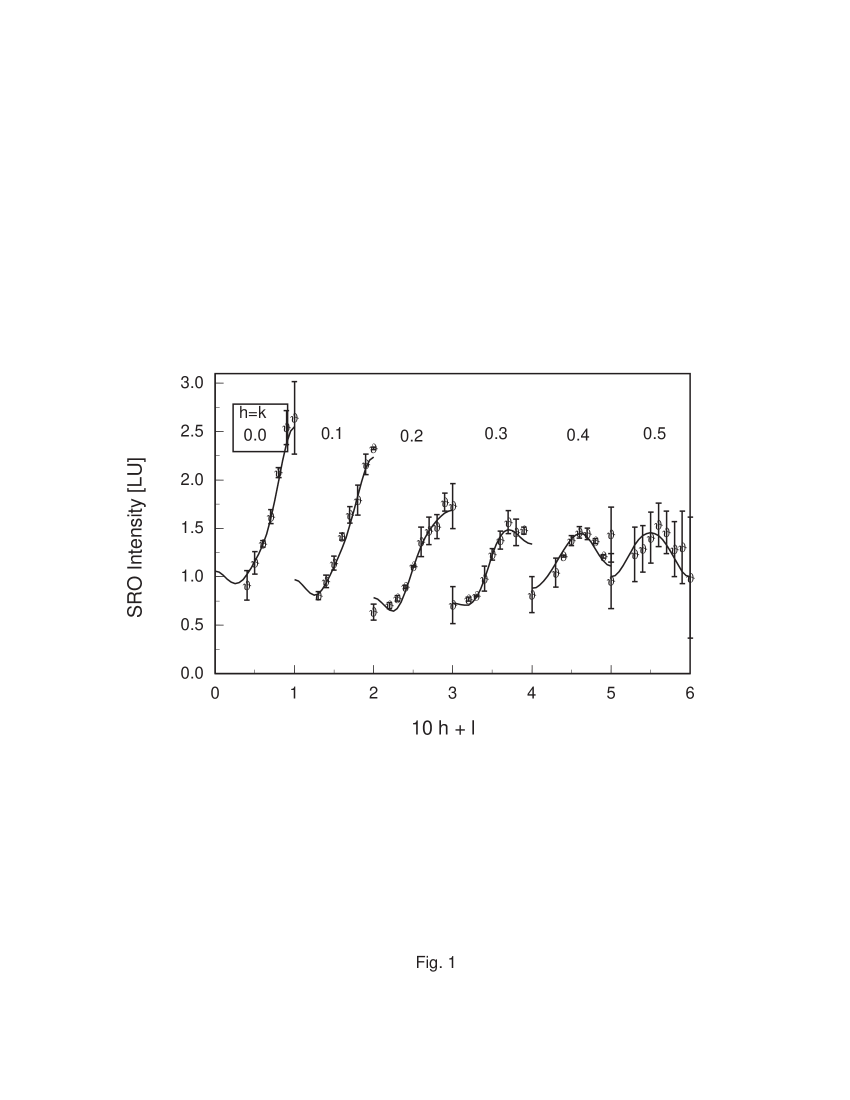
FIG. 1.: Experimental short-range order diffuse intensity (symbols) and the fit (solid line) obtained using 8 shells of Warren-Cowley short-range parameters $\alpha_{n}$.

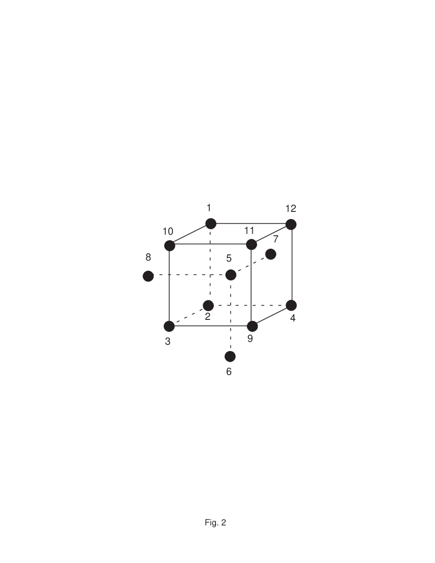
FIG. 2.: Clusters used in the three different approximations of the Cluster Variation Method: Tetrahedron (T) approximation (points 1-2-5-7); Cube-Octahedron (C-O) approximation combining the body-centered cube (points 1-2-3-4-5-9-10-11-12) and octahedron (points 2-3-4-5-6-9) clusters; and the Cube-Rhombohedron-Octahedron (C-R-O) approximation combining, in addition to the two clusters in the Cube-Octahedron approximation, the rhombohedron labeled 1 through 8.

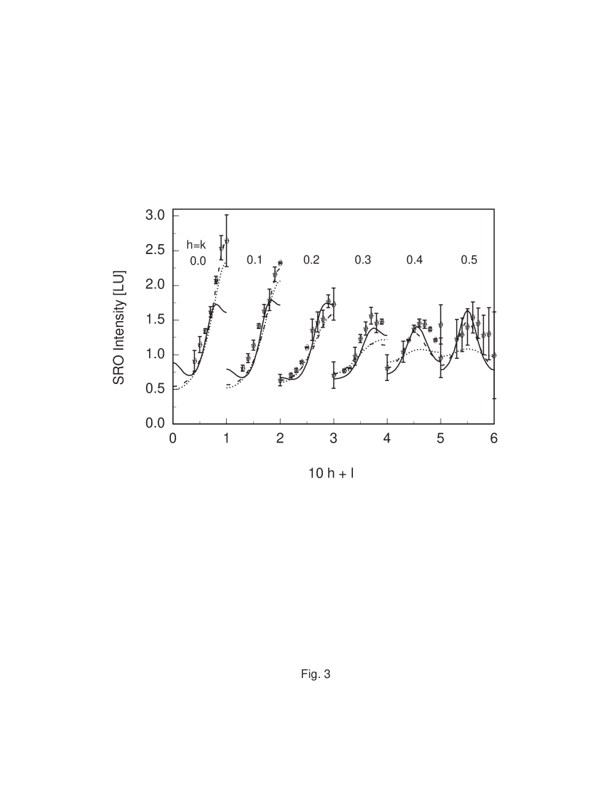
FIG. 3.: Short range order diffuse intensity obtained using the real space inverse cluster variation method in three approximations: Tetrahedron (dotted line); Cube-Octahedron (dashed line) and Cube-Rhombohedron-Octahedron (full line). The symbols are experimental points.

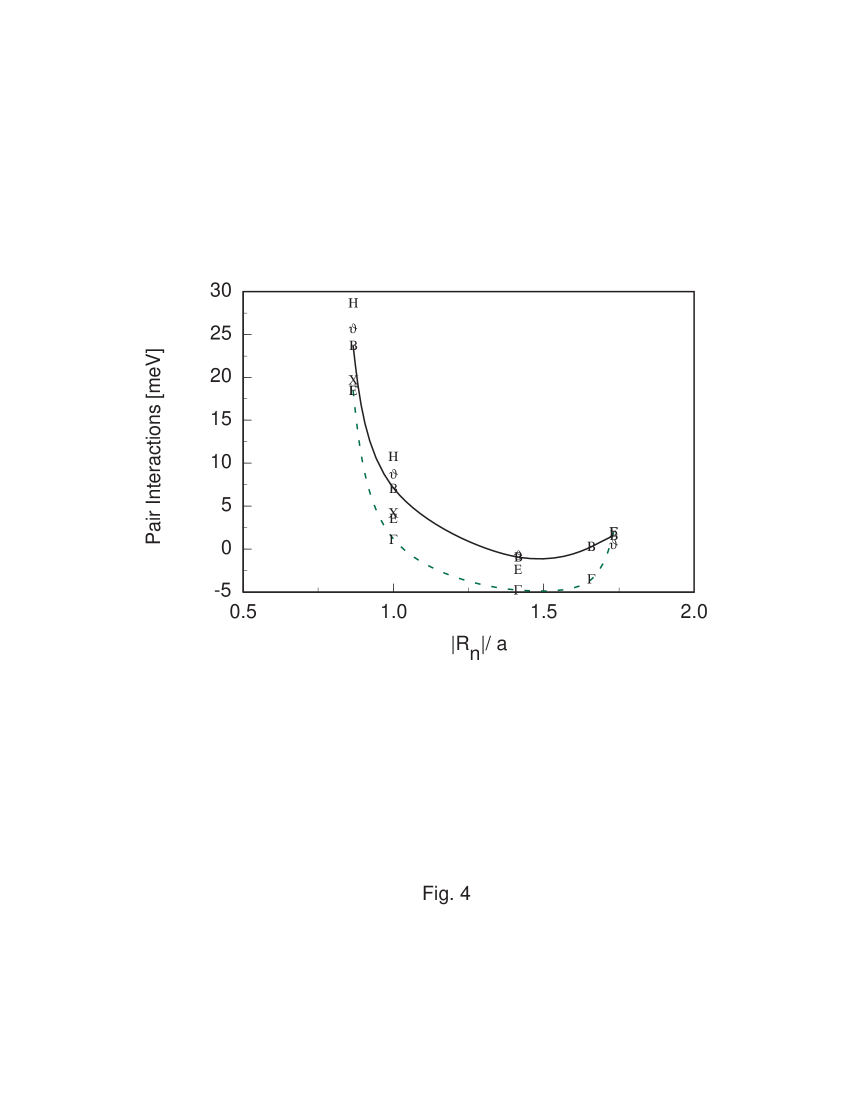
FIG. 4.: Effective pair interactions as function of distance, in units of the lattice constant $a$, obtained using the real space (open symbols) and the k-space (full symbols) methods described in the text. For each method, the cluster variation approximations used were the Tetrahedron (triangles), Cube-Octahedron (circles) and Cube-Rhombohedron-Octahedron (squares).

FIG. 5.: Short range order diffuse intensity obtained using the reciprocal space cluster variation method described in the text in three approximations: Tetrahedron (dotted line); Cube-Octahedron (dashed line) and Cube-Rhombohedron-Octahedron (full line). The symbols are experimental points.

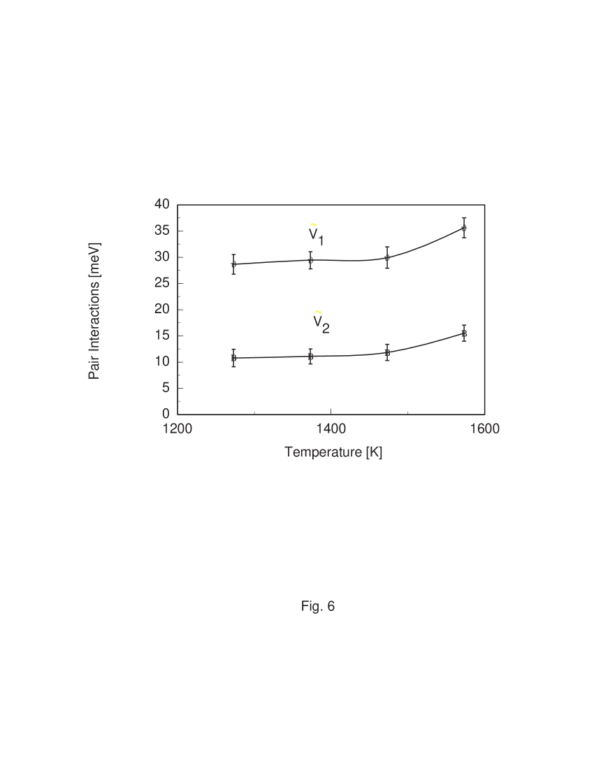
FIG. 6.: Temperature variation of the effective pair interactions for first (${\tilde{V}}_{1}$) and second (${\tilde{V}}_{2}$) neighbors obtained using the reciprocal space method in the Tetrahedron approximation.

TABLE I.: Pair interactions $\tilde{V}_{n}$ for ${\bf Fe}19.5at\%Al$ at $1273K$ obtained using real space inversion for three approximations of the cluster variation method. Errors in the estimated pair interactions are shown in parenthesis. Experimental Warren-Cowley short range order parameters are given in the second column. Those in the last column were calculated in the C-R-O approximation with the interactions of the C-O approximation.

	$Exp.$	$T$	$C-O$	$C-R-O$
n	$\alpha_{i}$	$\tilde{V}_{n}(meV)$	$\tilde{V}_{n}(meV)$	$\tilde{V}_{n}(meV)$	$\alpha_{i}$
1	-0.0943	$19.7(0.2)$	$18.5(0.3)$	$18.5(0.2)$	-0.0944
2	0.0114	$4.2(0.2)$	$3.6(0.2)$	$1.1(0.2)$	0.0113
3	0.0345		$-2.4(0.1)$	$-4.8(0.1)$	0.0351
4	0.0097			$-3.5(0.1)$	-0.0091
5	-0.0020		$2.0(0.1)$	$2.0(0.1)$	-0.0019

TABLE II.: Pair interactions $\tilde{V}_{n}$ and the corresponding Warren-Cowley short-range order parameters for ${\bf Fe}19.5at\%Al$ at $1273K$ obtained by fitting the SRO intensity in k-space using three approximations of the cluster variation method. Errors in the estimated pair interactions are shown in parenthesis.

	$T$		$C-O$		$C-R-O$
n	$\tilde{V}_{n}(meV)$	$\alpha_{n}$	$\tilde{V}_{n}(meV)$	$\alpha_{n}$	$\tilde{V}_{n}(meV)$	$\alpha_{n}$
1	$28.7(1.9)$	-0.1158	$25.7(4.7)$	-0.1107	$23.7(1.9)$	-0.1067
2	$10.8(1.7)$	-0.0044	$8.7(3.7)$	-0.0005	$7.1(0.4)$	0.0047
3			$-0.7(1.2)$	0.0326	$-0.9(0.1)$	0.0332
4					$0.3(0.1)$	-0.0080
5			$0.6(1.8)$	0.0076	$1.6(0.1)$	0.0016

REFERENCES

- [1] M. Bessière, Y.Calvayrac, S. Lefebvre, D. Gratias, and P. Cénédèse,J. Phys.47, 1961 (1986).
- [2] B.D. Butler, and J.B. Cohen, J. Appl. Phys. 65, 2214 (1986).
- [3] F. Solal, R. Caudron, F. Ducastelle, A. Finel, and A. Loiseau, Phys. Rev. Lett. 58, 2245 (1989).
- [4] V. Pierron-Bohnes, S. Lefebvre, M. Bessière, and A. Finel, Acta Metall. Mater. 34, 2701 (1990).
- [5] L. Reinhard, B. Schönfeld, G. Kostorz, and W. Bürer, Phys. Rev. B 44, 1727 (1990).
- [6] V. Pierron-Bohnes, M.C. Cadeville, A. Finel, and O. Schaerpf, J. Phys. I 1, 247 (1991).
- [7] L.Reinhard, J.L. Robertson, S.C. Moss, G.E. Ice, P. Zschack, and C.J. Sparks, Phys. Rev. B 45, 2262 (1992).
- [8] J.M. Cowley, J.Appl. Phys. 21, 24 (1950).
- [9] M.A. Krivoglaz, Theory of X-Ray and Thermal Neutron Scattering by Real Crystals, Plenum, New York, 1969.
- [10] P.C. Clapp and S.C. Moss Phys. Rev.142, 418 (1966); ibid 171, 754 (1968).
- [11] S.C. Moss and P.C. Clapp Phys. Rev. 171, 764 (1968).
- [12] W.L. Bragg and E.J. Williams, Proc. Roy. Soc. A 145, 69 (1934).
- [13] R. Kikuchi, Phys. Rev. 81, 988 (1951).
- [14] J.M. Sanchez Physica 111A, 200 (1982).
- [15] T. Mohri, J.M. Sanchez, and D. de Fontaine Acta Metall. 33, 1463 (1985).
- [16] D. Gratias and P. Cénédèse J. de Physique 46, C9-149 (1985).
- [17] F. Livet, Acta Metall. 35, 2915 (1987); F. Livet and M. Bessière, J. Phys. 48, 1703 (1987).
- [18] W. Schweika and H.G. Haubold, Phys. Rev. B 37, 9250 (1988).
- [19] V. Pierron-Bohnes, C. Leroux, J.P. Ambroise, A. Menelle, P. and Bastie, Phys Stat. Solidi (a) 116, 529 (1989).
- [20] B. Borie and C.J. Sparks, Acta Cryst. A 27, 198 (1971).
- [21] J.M. Sanchez, F. Ducastelle and D. Gratias, Physica 128A, 334 (1984).
- [22] J.M. Sanchez Phys.Rev. B 48, 13 (1993).