Layered Multishift Coupling
for use in Perfect Sampling Algorithms
(with a primer on CFTP)

Abstract.

In this article we describe a new coupling technique which is useful in a variety of perfect sampling algorithms. A multishift coupler generates a random function $f()$ so that for each $x\in{\mathbb{R}}$, $f(x)-x$ is governed by the same fixed probability distribution, such as a normal distribution. We develop the class of layered multishift couplers, which are simple and have several useful properties. For the standard normal distribution, for instance, the layered multishift coupler generates an $f()$ which (surprisingly) maps an interval of length $\ell$ to fewer than $2+\ell/2.35$ points — useful in applications which perform computations on each such image point. The layered multishift coupler improves and simplifies algorithms for generating perfectly random samples from several distributions, including the autogamma distribution, posterior distributions for Bayesian inference, and the steady state distribution for certain storage systems. We also use the layered multishift coupler to develop a Markov-chain based perfect sampling algorithm for the autonormal distribution.

At the request of the organizers, we begin by giving a primer on CFTP (coupling from the past); CFTP and Fill’s algorithm are the two predominant techniques for generating perfectly random samples using coupled Markov chains.

1. Primer on Coupling from the Past

1.1. Markov chain Monte Carlo

For many applications in statistical physics, computer science, and Bayesian inference, it is very useful to generate random structures according to some pre-specified distribution. Sometimes there is a direct random generation method, such as with percolation, random permutations, or Gaussian random variables. But often the state spaces are more complicated and there is no known direct sampling method, as is the case for random independent sets of a graph, random linear extensions of a partially ordered set, or random contingency tables. To sample from state spaces such as these, people typically rely upon Markov chains. There is some natural randomizing operation, which given an input state, produces a randomly modified output state. If the input state is already distributed according to the desired distribution, then so is the output state. Under mild conditions, if sufficiently many randomizing operations are performed, then the final state will be distributed in approximately the desired distribution.

The computer which simulates the Markov chain doesn’t have any idea what “sufficiently many” means. This may mean one of the following.

• The computer keeps simulating the Markov chain forever. This may be OK when doing mathematics, but it is not a practical approach to MCMC.

• The human guesses how many steps must be enough. The guess could be bad.

• The human applies spectral analysis or other mathematical techniques to rigorously determine how many steps are enough. Obtaining rigorous bounds has been an active area of research in the past decade, and there have been some notable successes. More than one person has been elected to the National Academy of Sciences for work in this area. But by and large this remains a hard problem, and many (if not most) Markov chains of practical interest have so far failed to succumb to rigorous analysis.

• The human writes code to measure various autocorrelation functions, thereby allowing the computer to heuristically guess how many steps are enough. This method is the workhorse for MCMC in physics and statistics. In the absence of a better option, it gets the job done. But no matter how good the heuristics are, one can never be completely sure that they did the job correctly, and the allegedly random samples produced could be quite biased.

• The computer (rigorously) figures out on its own how long to run the Markov chain. When it is possible to do this, life is simplified for the experimenter. The two predominant methods for doing this are known as “coupling from the past” (CFTP) (Propp and Wilson, 1996) and Fill’s algorithm (Fill, 1998a). The first of these methods is the topic of this primer; additional information on the second is given by Fill, Machida, Murdoch, and Rosenthal (1999).

1.2. Randomizing operations, pairwise couplings, and Markov chains

Typically a randomizing operation is expressed as a deterministic function $\phi$ that takes two inputs, the input state $X_{t}$ at time $t$ and some intrinsic randomness $U_{t}$, and returns the modified output state $X_{t+1}=\phi(X_{t},U_{t})$. One can think of $\phi$ as representing a piece of C code or Lisp code, and $U_{t}$ as representing the output of the pseudorandom number generator. It is assumed that the $U_{t}$’s are mutually independent. Conceptually it is convenient to combine $\phi$ and $U_{t}$ into a single random function $f_{t}$ defined by $f_{t}(x)=\phi(x,U_{t})$. The randomizing operation is assumed to preserve the desired distribution $\pi$ from which we wish to sample: if $X_{t}$ is distributed according to $\pi$ and $U_{t}$ is random, then $X_{t+1}$ is also distributed according to $\pi$.

Applying the randomizing operation to a given state is equivalent to running the Markov chain one step from that state. There can be many different randomizing operations that are consistent with a given Markov chain.

Just as a toy example, suppose that the state space consists of the integers from $0$ to $n$, that $U_{t}$ is $+1$ or $-1$ with probability $1/2$ each, and $\phi$ is defined by

$$\phi(x,u)=\begin{cases}x+u&0\leq x+u\leq n\\ 0&x+u<0\\ n&x+u>n\end{cases}.$$

Then it is easy to check that the only distribution $\pi$ preserved by these randomizing operations is the uniform distribution on $0,1,\ldots,n$.

A different randomizing operation $\psi$ might flip $n+1$ different coins, and use the $x$th coin flip when computing $\psi(x,u)=\phi(x,u_{x})$. While these two randomizing operations are different, they give rise to the same Markov chain. For CFTP, the choice of randomizing operation is as important as the Markov chain itself.

A pairwise coupling is a method for updating a pair of states so that the evolution of either state by itself is described by the Markov chain. Randomizing operations are also sometimes called “simultaneous couplings” or “grand couplings”, since the specified how any group of states will evolve. There are exceptions (see e.g. § 1.6.1), but a large fraction of the pairwise couplings encountered in practice extend naturally to grand couplings / randomizing operations. For the purposes of CFTP, we will principally be interested in randomizing operations.

1.3. CFTP: Sampling with and then without an oracle

Suppose that we have an oracle which returns perfectly random samples distributed according to $\pi$. Such oracle would make life easy for someone doing Monte Carlo experiments, if not for the fact that it charges $20 for each sample requested of it. Since we do not have an unlimited budget, we would like to make use of our randomizing operation, which is essentially free, and thereby reduce our dependence upon the oracle.

To this end, consider experiment $A_{T}$ given below:

• Pay $20 to the oracle to draw $X_{-T}$ from $\pi$

• For $t=-T$ upto $-1$

• Compute $X_{t+1}:=\phi(X_{t},U_{t})$

• Output $X_{0}$

Because the distribution $\pi$ is preserved by the randomizing operation, by induction follows that the output state $X_{0}$ is distributed exactly according to $\pi$. Next consider experiment $B_{T}$ given below:

• Look at $U_{-T},U_{-T+1},\ldots,U_{-1}$

• If there is only one possible value for $X_{0}$

• Then

• Output $X_{0}$

• Else

• Pay $20 to the oracle to draw $X_{-T}$ from $\pi$

• For $t=-T$ upto $-1$

• Compute $X_{t+1}:=\phi(X_{t},U_{t})$

• Output $X_{0}$

If we’re lucky, experiment $B_{T}$ does not need to pay the oracle $20. Note that experiment $B_{T}$ always returns precisely the same answer that experiment $A_{T}$ does, provided that the same random values $U_{t}$ are used. From this we see that the output of experiment $B_{T}$ is distributed exactly according to $\pi$, provided that the random values $U_{t}$ used in the second part are the same values used in the first part of the procedure. Using fresh random values in the second part of the procedure is a bad idea that would cause the output state to be biased. Also note that the running time of experiment $B_{T}$ is a random variable which may be correlated with the output state. Thus repeatedly running, interrupting, and restarting the procedure is also a bad idea that would introduce bias — much better to let the procedure finish running and return its answer.

We return to our toy example to see how one might conduct experiment $B_{T}$ in practice. Figure 1 shows two possible outcomes of experiment $B_{10}$.

Figure 1. The outcome of experiment $B_{10}$ using two different sequences of the coins $U_{-10},\ldots,U_{-1}$. The horizontal axis represents time. In the first example, the coins determine the final state $X_{0}$, so there is no need to consult the oracle, and state $3$ is output. In the second example, the coins restrict the possible values of $X_{0}$ but do not determine it. The oracle is then consulted (for a fee of $20), and returns state $1$, which gets sent to state $2$ (the output) by the coins. In both cases we only had to track the top-most and bottom-most trajectories (rather than all of them) to see if the coins determine state $X_{0}$.

In the first example the random choices of $U_{-10},\ldots,U_{-1}$ were $+1$, $-1$, $-1$, $+1$, $+1$, $-1$, $+1$, $+1$, $+1$, $-1$. Every possible starting value for state $X_{-10}$ was tried, and for each of these starting values the final state $X_{0}$ was $3$. Since the given choices of $U_{-10},\ldots,U_{-1}$ determine $X_{0}$, the oracle was not consulted, and the final output state was $3$.

This example also illustrates a convenient property of what are known as “monotone Markov chains”. The state space comes equipped with a partial order $\preceq$ with a biggest state $\hat{1}$ and a smallest state $\hat{0}$ such that $\hat{0}\preceq x\preceq\hat{1}$ for all states $x$. In this toy example the partial order $\preceq$ is the usual order $\leq$ on integers, $\hat{1}=4$, and $\hat{0}=0$. A randomizing operation on a partially ordered set is monotone if $x\preceq y$ implies $\phi(x,u)\preceq\phi(y,u)$. For monotone Markov chains it is particularly easy to test if the $U_{t}$’s determine $X_{0}$: apply the randomizing operations starting from $X_{-T}=\hat{0}$ and then from $X_{-T}=\hat{1}$. If $f_{-1}(\cdots f_{-T}(\hat{0})\cdots)=f_{-1}(\cdots f_{-T}(\hat{1})\cdots)$, then no matter what starting value for $X_{-T}$ that the oracle would have selected, the final value for $X_{0}$ is just $f_{-1}(\cdots f_{-T}(\hat{1})\cdots)$. So it is only necessary to test two possible starting values rather than all of them.

In the second example a different set of random choices of $U_{-10},\ldots,U_{-1}$ is used. In this case $U_{-10},\ldots,U_{-1}$ did not determine $X_{0}$, so $20 was paid to the oracle, which then assigned $X_{-10}=1$. Applying the randomizing operations specified by $U_{-10},\ldots,U_{-1}$ resulted in the final state $X_{0}=2$, which was the output.

In order to reduce the chance that we have to resort to paying $20 to the oracle, we should pick a large value of $T$ when doing experiment $B_{T}$, since that would increase the probability that $U_{-T},\ldots,U_{-1}$ determine $X_{0}$. But if we pick an excessively large value of $T$, we’d rather not spend time looking at all the $U_{t}$’s if the last several of them by themselves determine $X_{0}$. We could look at the last several $U_{t}$’s and see if they determine $X_{0}$. If not, we can continue to look at progressively more of the $U_{t}$’s to see if they determine $X_{0}$. If we are unlucky and $U_{-T},\ldots,U_{-1}$ fail to determine $X_{0}$, then we resort to paying $20 to the oracle. This strategy is expressed more formally as experiment $C_{T}$ given below. It is evident that experiment $C_{T}$ and experiment $A_{T}$ will return the same answer provided that they use the same values of $U_{-T},\ldots,U_{-1}$ and the oracle return the same sample (if asked to do so). Thus experiment $C_{T}$ returns a random sample distributed exactly according to $\pi$, assuming of course that each time it looks at a given random variable $U_{t}$, it sees the same value. For this reason people often stress the importance of “re-using the same random coins”.

• If $U_{-1}$ determines $X_{0}$

• Then Output $X_{0}$

• Else If $U_{-2},U_{-1}$ determine $X_{0}$

• Then Output $X_{0}$

• Else If $U_{-4},U{-3},U_{-2},U_{-1}$ determine $X_{0}$

• Then Output $X_{0}$

• $\vdots$

• Else If $U_{-2^{\lceil\log_{2}T\rceil-1}},\ldots,U_{-1}$ determine $X_{0}$

• Then Output $X_{0}$

• Else If $U_{-T},\ldots,U_{-1}$ determine $X_{0}$

• Then Output $X_{0}$

• Else

• Pay $20 to the oracle to draw $X_{-T}$ from $\pi$

• For $t=-T$ upto $-1$

• Compute $X_{t+1}:=\phi(X_{t},U_{t})$

• Output $X_{0}$

Coupling from the past is experiment $C_{\infty}$, which is defined by

$$\text{CFTP}=\text{Experiment $C_{\infty}$}=\lim_{T\rightarrow\infty}\text{Experiment $C_{T}$}.$$

Since all experiments $C_{T}$ (for large enough $T$) start out by doing the same thing, taking this sort of limit makes sense. Experiment $C_{\infty}$, which is re-expressed below, has the convenient property that it never consults the oracle. CFTP is also illustrated in Figure 2.

• $T:=1$

• While $U_{-T},\ldots,U_{-1}$ do not determine $X_{0}$

• $T:=2*T$

• Output $X_{0}$

Figure 2. Illustration of CFTP in the monotone setting. Shown are the heights of the upper and lower trajectories started at various starting times in the past. When a given epoch is revisited later by the algorithm, it uses the same randomizing operation.

1.4. Questions and answers

When explaining CFTP to an audience, there are invariably many questions. Included below are some of these questions together with their answers.

Q: If we always end up in state $3$ no matter where we start, then how is that a random sample?

A: For a given particular sequence of coin flips, every possible starting state ends up in state $3$. But for a different (random) sequence of coin flips, every possible starting state may end up in a different final state at time $0$.

Q: What if we just run the Markov chain forward until coalescence?

A: Consider the toy example of the previous section. Coalescence only occurs at the states $0$ and $n$, so the result would be very far from being distributed according to $\pi$.

Q: What happens if we use fresh coins rather than re-using the same coins?

A: Consider the toy example of the previous section, and set $n=2$ (so the states are $0,1,2$). Then one can check that the probability of outputting state $1$ has a binary expansion of $0.0010010101001010101010101001\ldots$, which is neither rational nor very close to $1/3$.

Q: Rather than doubling back in time, what if we double forward in time, and stop the Markov chain at the first power of $2$ greater than or equal to the coalescence time?

A: As before, set $n=2$ in our toy example. One can check that the probability of outputting state $1$ is $1/6$ rather than $1/3$.

Q: What if we instead …

A: Enough already! There do exist other ways to generate perfectly random samples, but the only obvious change that can be made to the CFTP algorithm without breaking it is changing the sequence of starting times in the past from powers of $2$ to some other sequences integers.

Q: If coupling forwards in time doesn’t work, then why does going backwards in time work?

A: If you did not like the first explanation, then another way to look at it is that a virtual Markov chain has been running for all time, and so today the state is random. If we can (with probability 1) figure out today’s state by looking at some of the recent randomizing operations, then we have a random state.

Q: If going backwards in time works, then why doesn’t going forwards in time work?

A1: There is a way to obtain perfectly random samples by running forwards in time (Wilson, 1999), but none of the obvious variations described above work.

A2: CFTP determines the state at a deterministic time, any one of which is distributed according to $\pi$. The variations suggested above determine the state at a random time, where that time is correlated with the moves of the Markov chain in a complicated way, and these correlations mess things up.

Q: Why did you step back by powers of 2, when any other sequence would have worked?

A: For efficiency reasons. Let $T^{*}$ be the best time in the past at which to start, i.e. the smallest integer for which starting at time $-T^{*}$ leads to coalescence. By stepping back by powers of $2$, the total number of Markov chain steps simulated is never larger than $4T^{*}$ (and closer to $2.8T^{*}$ “on average”); see (Propp and Wilson, 1996, §5.2). If we had stepped back by one each time, then the number of simulated steps would have been $\binom{T^{*}}{2}\approx\frac{1}{2}(T^{*})^{2}$. If we had stepped back quadratically, then the number of simulated steps would have been about $\frac{1}{3}(T^{*})^{3/2}$. For this reason some people prefer quadratic backoff when $T^{*}$ is fairly small (Møller, 1998).

Q: So you need the state space to be monotone?

A: That would certainly be very useful, but there are many counterexamples to the proposition that is necessary. See § 1.6.

Q: Can you do CFTP on Banach spaces?

A: I don’t know. Depends on whether or not you can figure out the state at time 0.

Q: Where’s the proof of efficiency?

A: In the monotone setting, loosely speaking, CFTP is efficient whenever the Markov chain mixes rapidly; see § 1.6.1. There also proofs of efficiency for certain non-monotone settings.

Q(?): But you still need to analyze the mixing time, since otherwise you won’t know how long it will take.

A: Wrong. The principal advantage of using CFTP (or Fill’s algorithm) is that you don’t need these a priori mixing time bounds in order to run the algorithm, collect perfectly random samples, and carry on with the rest of the research project. The fact that these are perfectly random samples is icing on the cake. (But I still think that mixing time bounds are interesting.)

Q: But sampling spin glass configurations is NP-hard.

A: The spin-glass Markov chain that you’re using is probably very slowly mixing in the worst case. CFTP will not be faster than the mixing time of the underlying Markov chain.

Q: Is CFTP like a ZPP or Las Vegas algorithm for random sampling?

A: “Yes” for Las Vegas, “sometimes” for ZPP. [A Las Vegas algorithm uses randomness to compute a deterministic function. The running time is a random variable, but with probability 1 it returns an answer, and when it does so, the answer is correct. A Monte Carlo algorithm in contrast does not guarantee a correct answer. A problem is in ZPP if it can be solved by polynomial expected time Las Vegas algorithm.]

Q: Could you make a hybrid algorithm, which starts out by doing CFTP, but then does something different if CFTP starts to take a long time?

A: Yes. This would be like experiment $C_{T}$.

Q: What’s the probability that CFTP takes a long time?

A: The tail distribution of the running time decays geometrically. More can be said if the Markov chain is monotone, see § 1.6.1.

Q: What if I don’t want to wait for $10^{70}$ years. Does this make CFTP biased? Is it really better than forwards coupling?

A1: The answer to the second question is yes. How long are you willing to wait? With forward coupling, that’s how long you wait. With CFTP your average waiting time is probably much smaller.

A2: The answer to the first question depends on what you mean by “biased”. No-one disputes that the systematic bias is zero. The so-called “user-impatience bias” (the effect of an impatient user interrupting a simulation and progress) is a second order effect that pertains to most random sampling algorithms that most people would not call biased.

A3: If you’re genuinely concerned about the quality of your random samples, you should first spend time picking a good pseudo-random number generator.

A4: Anyone concerned about “user-impatience bias” should be equally concerned about “user-patience bias”: if an experimenter run simulations until some deadline, and then lets the last one finish before quitting, then the resulting collection of samples is biased to contain more samples that take a long time to generate. But if the experimenter instead aborts the last simulation (unless there are no samples so far, in which case (s)he lets it finish), then the resulting collection of samples is unbiased. See (Glynn and Heidelberger, 1990).

Q: Can you quantify the user-impatience bias?

A: If you generate $N$ samples before your deadline, and then average some function of these samples, the bias is at most $\Pr[N=0]$. If you do something sensible in the event that $N=0$, the bias will be even less. See (Glynn and Heidelberger, 1990).

1.5. Historical remarks and further reading

Monotone-CFTP was developed in 1994, although related ideas had appeared in the literature prior to that time. Asmussen, Glynn, and Thorisson (1992) and Lovász and Winkler (1995) (see also (Aldous, 1995)) had given algorithms for generating perfectly random samples from the steady-state distribution of any finite Markov chain; CFTP is generally more efficient at this task (Propp and Wilson, 1998b). Letac (1986) noticed that if one composed random maps backwards in time rather than forwards in time, then applying these maps to a given state typically led to pointwise convergence rather than just convergence in distribution. (Diaconis and Freedman (1999) survey this and related work.) But the random maps were composed backwards in time forever, and little attention was given to the question of how or if one could stop the process and obtain a random sample in finite time; one researcher in this area expressed surprise and disbelief upon first learning that this was possible (Foss, 1996). Notable exceptions are the Aldous (1990) / Broder (1989) algorithm for random spanning trees, which reverses time when building the tree, and an algorithm for the “dead leaves model” in which leaves fall up from the ground rather than down from the sky (see (Jeulin, 1997), (Kendall and Thönnes, 1999), and http://www.warwick.ac.uk/statsdept/Staff/WSK/dead.html). In both these cases a Markov chain is run backwards in time. Monotone-CFTP and nearly all subsequent versions of CFTP compose their randomizing operations forwards in time but starting from ever distant times in the past. Johnson (1996) independently studied monotone couplings, but did not couple them from the past. Monotone-CFTP may be applied to a surprisingly wide variety of Markov chains (see § 1.6.1), and after its success, many people started looking at other coupling methods that could be used with CFTP (see § 1.6).

For more in-depth explanations of the ideas described so far, the reader is referred to (Propp and Wilson, 1996) or the expository articles (Propp, 1997) or (Propp and Wilson, 1998a). Some people prefer the explanation of CFTP in (Fill, 1998a). Subsequent to the writing of this primer on CFTP, the author became aware of two additional expositions on perfect sampling with Markov chains: (Dimakos, 1999) and (Thönnes, 1999).

A more recent development is an algorithm related to CFTP but for which the Markov chain is run forwards in time and never restarted further back in the past (Wilson, 1999).

Additional information on perfect sampling is available at http://dimacs. rutgers.edu/~dbwilson/exact/.

1.6. Overview of common coupling methods

1.6.1. Monotone coupling

We saw the method of monotone coupling when looking at the toy example in § 1.3. Just as a reminder, the state space comes equipped with a partial order $\preceq$ with a biggest state $\hat{1}$ and a smallest state $\hat{0}$ such that $\hat{0}\preceq x\preceq\hat{1}$ for all states $x$. A randomizing operation on a partially ordered set is monotone if $x\preceq y$ implies $\phi(x,u)\preceq\phi(y,u)$. To test if the randomizing operations determine $X_{0}$, it is only necessary to apply them to the two starting values $\hat{0}$ and $\hat{1}$. Examples of monotone couplings include

• The Fortuin-Kasteleyn random cluster model with $q\geq 1$. These can be used to generate random configurations from dimer Ising and Potts models (Fortuin and Kasteleyn, 1972).

• Dimer models on bipartite planar graphs. These include domino tilings (Levitov, 1990; Zheng and Sachdev, 1989) and lozenge tilings (Blöte and Hilhorst, 1982). See also (Conway and Lagarias, 1990; Thurston, 1990; Propp, 1993).

• Ice models, including the 6-vertex model (van Beijeren, 1977) and the 20-vertex model.

• The hard core model on bipartite graphs (random independent sets) (Kim, Shor, and Winkler, 1995).

• The Widom-Rowlinson model with 2 types of particles (Häggström, van Lieshout, and Møller, 1999). This is actually a special case of the hard core model.

• Linear extensions of a 2D partially ordered set (Felsner and Wernisch, 1997).

• Attractive area interaction point process (Kendall, 1998).

• Certain queueing systems (Lund and Wilson, 1997).

• The beach model (Nelander, 1998).

• Statistical analysis of DNA using the “M1-M$m$” model (Muri, Chauveau, and Cellier, 1998).

• A mite dispersal model (Straatman, 1998).

• Slice samplers (Mira, Møller, and Roberts, 1998).

• The autonormal distribution (§ 3).

When using Fill’s algorithm, a somewhat weaker notion of monotonicity is sufficient. Rather than a monotone randomizing operation, as is needed for monotone CFTP, it is sufficient to have a monotone pairwise coupling (Fill, 1998a). Rather than produce a whole random map which is both monotone and marginalizes to a given Markov chain, it is sufficient to specify how any two given states may be updated together in a monotone fashion. Fill and Machida (1998) show that there are Markov chains with a pairwise monotone update rule but with no monotone randomizing operation, but so far there haven’t been any such examples where someone wanted to sample from the steady state distribution.

When monotone couplings are used either with CFTP or Fill’s algorithm, the running time of the algorithm has been rigorously related to the mixing time of the Markov chain (see Propp and Wilson (1996) and Fill (1998a)). For CFTP the relevant notion of mixing time $T_{\operatorname{mix}}$ is the “total variation threshold time”, which is what most people mean by the phrase “mixing time”. For Fill’s algorithm, the relevant notion of mixing time is $T_{\operatorname{sep}}$, the “separation distance threshold time”. We won’t define these terms here, but the interested reader can read about them in (Aldous and Fill, 199X).

Let $\ell$ denote the length of the longest chain within the partially ordered state space. Then the time to coalescence (or how far back in the past that you need to start) $T^{*}$ has its expected value bounded by

$$T_{\operatorname{mix}}/e\leq E[T^{*}]\leq 2T_{\operatorname{mix}}(1+\ln\ell),$$

where $e=2.71828\ldots$ (Propp and Wilson, 1996). For some examples (including lozenge tilings of a hexagonal region) it is possible to determine both the mixing time in the coupling time to within constants, and for these cases the coupling time does not contain an extra $\log$ factor (Fill, 1998b) (Wilson, 1997). But it is also possible to construct examples for which the $\log$ factor does appear in the coupling time (Lund and Wilson, 1997).

The expected coupling time for Fill’s algorithm can be bounded by

$$E[T^{*}]=\Theta(T_{\operatorname{sep}}).$$

In fact, the cumulative distribution function of the coupling time plus the separation distance as a function of time add up to the constant function $1$ Fill (1998a). For comparison with CFTP, we note that in general $T_{\operatorname{sep}}\geq T_{\operatorname{mix}}$, and that for reversible Markov chains $T_{\operatorname{sep}}=\Theta(T_{\operatorname{mix}})$.

Thus for monotone Markov chains, from a running time standpoint, there is little or no reason not to use one of these two perfect sampling algorithms.

1.6.2. Anti-monotone coupling and Markov random fields

Mathematicians use the term “Markov random field” where physicists use the term “spin system” where statisticians use the term “conditionally specified model”. A Markov random field is a collection of random variables (or spins) defined at the vertices (or sites) of a graph; the edges of the graph contain information about the correlations between the random variables. If the values of all the spins except one are specified, then the conditional distribution of the remaining spin is a function only of that spin’s neighbors. One of the more frequently used Markov chains on spin systems is the “single-site heat bath”, also known as “Gibbs sampling”. The Markov chain picks a site, either at random or in sequence, and then randomizes the spin at that site by drawing from its conditional distribution when the remaining spins are held fixed.

A spin system is attractive if there is a partial order on the values of the spins, such that increasing the values of the spins only increases the conditional distribution of the spin at a given site. Most of the examples of monotone coupling given in § 1.6.1 are in fact instances of attractive spin systems.

A spin system is repulsive if there is a partial order on the values of the spins, such that increasing the values of the spins only decreases the conditional distribution of the spin at a given site. “Anti-monotone coupling” was first used by Kendall (1998) and Häggström and Nelander (1998) to generate perfectly random samples from repulsive spin systems. Instances of these repulsive systems include

• The repulsive area interaction point process (Kendall, 1998).

• The hard-core model on non-bipartite graphs (Häggström and Nelander, 1998).

• The Ising antiferromagnet (Häggström and Nelander, 1998).

• Fortuin-Kasteleyn random cluster model with $q<1$ (Häggström and Nelander, 1998).

• The autogamma distribution (Møller, 1999).

With anti-monotone coupling with Gibbs sampling, one maintains at each site an upper bound and a lower bound for the spin at that site. If there is a smallest and a biggest spin value, then these become the initial lower bound and upper bound; see § 1.9 if there is no smallest or largest spin value. In contrast with attractive spin systems, there is no particular reason for the configuration consisting entirely of the lower bounds or entirely of the upper bounds to have positive probability. For instance, for the hard-core model, the configuration consisting of all upper bounds will have particles too close to each other (unless there are no edges), and will thus have probability 0. But this is irrelevant for our purposes: the bounds on the spin values specify a superset of the possible states that the Markov chain may be in. When doing a Gibbsian update at a given site, when determining the upper bounds at the neighboring sites are used when determining the new lower bound at that site, and vice versa.

The area interaction point process requires further explanation because there are infinitely many sites. The configurations tend to be sparse because there are only two possible spin values, and (normally) the spins at all but finitely many sites are of the first type. Kendall (1998) used his method of dominated CFTP (see § 1.9.3) together with anti-monotone coupling to sample from this distribution.

For the autogamma distribution, the possible spin values are the non-negative reals. See § 1.9.1 for remarks about upper-bounding the possible spin values.

Häggström and Nelander (1998) and Huber (1998) independently generalized the approach of anti-monotone coupling on repulsive systems to more generic Markov random fields. At each site, one still maintains the set of possible values of the spin at that site, but that set can no longer be represented by an interval specified by a lower bound and upper bound. The sense of possible spins at each site collectively define some abstract high-dimensional box which contains the possible states of the Markov chain. Updating the set of possible values of the spin at a given site becomes more complicated than in the anti-monotone setting, and good coupling methods are essential to making it work. The reader is referred to the original articles to see how the following examples are done.

• Random $q$-colorings (Häggström and Nelander, 1998; Huber, 1998).

• The Widom-Rowlinson model with more than two particle types (Häggström and Nelander, 1998).

1.6.3. Techniques for Bayesian inference

Murdoch and Green (1998) and Green and Murdoch (1999) developed a number of techniques that are suited for applying CFTP to sampling from the (continuous) posterior distributions associated with Bayesian inference problems. Here the state space is typically ${\mathbb{R}}^{d}$. At each time step the algorithm maintains a superset of the possible states of the Markov chain where the superset is represented by a finite collection of boxes together with a finite set of points. It is not possible to do justice to these coupling techniques within a short primer on CFTP, so the reader is referred to their original articles.

1.7. Coupling ex post facto

Here we review “ex post facto coupling”, a term introduced by Jim Fill. Later we explain the role that ex post facto coupling plays in Fill’s algorithm (§ 1.8) and “coupling into and from the past” (§ 1.9.3).

In ordinary pairwise coupling, a procedure takes as input two states $x$ and $y$ and produces two states $x^{\prime}$ and $y^{\prime}$ so that the transition from $x$ to $x^{\prime}$ and the transition from $y$ to $y^{\prime}$ both look like they were produced from a given Markov chain.

• ($x^{\prime}$,$y^{\prime}$) := PairWiseCoupling($x$,$y$)

Usually there are additional constraints on useful couplings, such as a monotonicity constraint or a contraction property. In ex post facto coupling, somebody else generates the $x^{\prime}$ according a Markov update on $x$, and your job is to take $x$, $x^{\prime}$, $y$, and generate a random $y^{\prime}$ so that the distribution of $x^{\prime},y^{\prime}$ given $x,y$ is governed by the original coupling.

• $x^{\prime\prime}$ := MarkovUpdate($x$)

• $y^{\prime\prime}$ := ExPostFactoCoupling($x$,$y$,$x^{\prime}$)

• /* DistributionOf($x^{\prime\prime}$,$y^{\prime\prime}$) == Distribution($x^{\prime}$,$y^{\prime}$) */

The same idea applies to random mappings.

• $F()$ := RandomMap()

• /* $F$ now defines a Markov update from any state $x$ */

Somebody else gives you a Markov chain step $(x,x^{\prime})$, and your job is to produce a random map $F$ from a given random map distribution, but conditioned on $F(x)=x^{\prime}$.

• $x^{\prime}$ := MarkovUpdate($x$)

• $F^{\prime}()$ := ExPostFactoMapping($x$,$x^{\prime}$)

• /* DistributionOf($F^{\prime}$) == DistributionOf($F$) */

• /* $F^{\prime}(x)$ == $x^{\prime}$ */

In other words, to do ex post facto coupling, we generate a random map or a random pairwise update, conditioned to satisfy a certain constraint. Since we just need to sample from a conditional distribution, in principle any coupling can be done ex post facto, but in practice this can be easier said than done.

1.8. Fill’s algorithm

Here we briefly describe Fill’s algorithm, and in particular the role that ex post facto coupling plays in it. For an explanation of why Fill’s algorithm works, see (Fill, 1998a) or (Fill, Machida, Murdoch, and Rosenthal, 1999).

In Fill’s algorithm, a single trajectory of the Markov chain is run forward in time for some number of steps $X_{0},\ldots,X_{n}$. This trajectory is treated as a sample path from the time-reversed Markov chain. Then a second trajectory (or in subsequent work, many trajectories) of the time-reversed Markov chain is coupled to it ex post facto. In other words, the time-reversal of the first trajectory together with all the new time-reversed trajectories have a joint distribution that is governed by some pre-specified coupling, conditioned upon the trajectory from $X_{n}$ being $X_{n},X_{n-1},\ldots,X_{1},X_{0}$. The state $X_{n}$ is returned if each of the time-reversed trajectories coalesced to $X_{0}$. Otherwise, the current experiment is discarded, and another (independent) one may be started. In the monotone setting, Fill’s algorithm only requires ex post facto coupling for a monotone pairwise coupling, but in more general settings, random maps are coupled ex post facto.

Fill’s algorithm is interruptible with respect to a deadline specified in terms of Markov chain steps, so the corresponding user-patience bias does not affect it. Code implementing the algorithm may or may not be interruptible with respect to a deadline specified in terms of time.

1.9. Methods for unbounded state spaces

Suppose that one has a partially ordered state space together with the monotone (or anti-monotone) randomizing operation. When doing monotone or anti-monotone CFTP, having a top state and bottom state is important, or at the very least, very useful. What can one do when there is no top state? The unboundedness of the state space can be similarly problematic when the couplings used do not rely on a partial order. In this section we describe the three main techniques that have been used when dealing with unbounded state spaces.

The method in § 1.9.1 extends the state space, the method in § 1.9.2 modifies the Markov chain, and the method and § 1.9.3 uses two coupled Markov chains, one going backwards in time in the other going forwards. For those familiar with the term “uniform ergodicity”, the method in § 1.9.1 requires uniform ergodicity, the method in § 1.9.2 produces a uniformly ergodic Markov chain starting from one that is non-uniformly ergodic, in the method and § 1.9.3 works with non-uniformly ergodic Markov chains. Despite the differences in approach and capabilities of the methods described in § 1.9.1 and § 1.9.3, they are both frequently referred to by the same term, namely “dominated CFTP”. The method in § 1.9.2 is comparatively new, so it is too early to tell whether or not it too will be referred to by this same term. We mention a fourth method in § 1.9.4.

1.9.1. Compactifying the state space

Adjoin a top state or bottom state if these are missing. Then the state spaces no longer unbounded. Trite as this solution may sound, in more than one case it works just fine and solves the problem, and it is much simpler than the approaches in § 1.9.3 and § 1.9.2 for dealing with unbounded state spaces.

Let us denote the newly adjoined top and/or bottom states by $+\infty$ and $-\infty$ respectively. Let $P_{x}(\cdot)$ denote the probability distribution of the next state of the Markov chain when it starts in state $x$. If there is some probability distribution which stochastically dominates $P_{x}(\cdot)$ for each $x$, then in the monotone case we can set $P_{+\infty}(\cdot)$ to be this distribution, and in the anti-monotone case we can set $P_{-\infty}(\cdot)$ to be this distribution. Similarly, if there is some probability distribution which is stochastically dominated by $P_{x}(\cdot)$ for each $x$, then we can define $P_{-\infty}(\cdot)$ or $P_{+\infty}(\cdot)$ in the monotone or anti-monotone cases respectively. If we adjoined $\pm\infty$ but then were unable to define $P_{\pm\infty}(\cdot)$, then one of the other methods (in § 1.9.2 or § 1.9.3) for dealing with unbound state spaces should be used.

In the new Markov chain the states $\pm\infty$ are transient, so the new steady-state distribution is the same as the old one, and we can proceed to sample from it using monotone or anti-monotone CFTP.

This approach is sometimes even easier done than said. For instance, when doing anti-monotone coupling with the autogamma distribution, the system is a repulsive spin system where the possible spin values are ${\mathbb{R}}^{+}$. Each spin variable $x_{i}$, conditional upon the remaining spins, is governed by a gamma distribution with shape parameter $\alpha_{i}$ which is then scaled down by a factor of

$$\beta_{i}+\sum_{j:j\neq i}\beta_{i,j}x_{j},$$ (*)

where $\beta_{i}>0$ and $\beta_{i,j}\geq 0$ (Møller, 1999). On any modern computer we can simply set the top state to be 1.0/0. This is because all modern computers conform to the IEEE 754 floating point arithmetic standard, which has built-in representations for both $+\infty$ and $-\infty$, and knows how to sensibly add numbers to infinity and divide numbers by infinity; see (Goldberg, 1990). No special code needs to be written to sample from $P_{+\infty}$ or otherwise deal with such a large top state: the code which computes the inverse scale parameter given by (* ‣ 1.9.1) and updates the range of possible spin values at a given site when the neighboring spin values are bounded by finite values will also work correctly when the neighboring spin values are bounded by $+\infty$ (thanks to IEEE arithmetic).

(Møller (1999) did not regard $+\infty$ to be a valid spin value, and used pages of detailed calculations to verify the anti-monotone CFTP still works. When we regard $+\infty$ as a valid spin value, it is obvious without calculation that anti-monotone CFTP still works.)

In other applications the computer hardware may not come prewired to deal with the $\pm\infty$ configurations as it did in the autogamma example, in which case this must be done in software. When figuring out whether or not the randomizing operations given by $U_{-T},U_{-T+1},\ldots,U_{-1}$ determine the state at time $0$, one piece of code could deal with the random map specified by $U_{-T}$, and another piece of code could deal with the subsequent $T-1$ random maps. From a mathematical standpoint there is no difference between the first randomizing operation and the subsequent ones. From an implementation standpoint, it is sometimes easier to write one piece of code optimized for the special case of the upper bound being $+\infty$ (and/or lower bound being $-\infty$), and a separate piece of code optimized for finite upper and lower bounds.

We remark that the continuous Widom-Rowlinson model is another example where the state space can be compactified by adjoining a top state $+\infty$ (consisting of all red points) and a bottom state $-\infty$ (consisting of all blue points). Häggström, van Lieshout, and Møller (1999) identified a finite “quasi-maximal” state big and a finite “quasi-minimal” state $-$big such that $P_{\infty}=P_{\texttt{big}}$ and $P_{-\infty}=P_{-\texttt{big}}$. Therefore they were able to represent $\pm\infty$ using $\pm\texttt{big}$ within their monotone-CFTP code. (Currently Møller advocates the approach, if not perspective, of the previous paragraph.)

1.9.2. Murdoch’s method of mixing with an independence sampler

This method is the next one to try if compactifying the state space does not work. This happens when the probability distribution has infinite tales, and a Markov chain started sufficiently far out in the tales can take arbitrarily long to reach the main part of the state space were the steady-state distribution $\pi$ is principally supported. The idea is to mix the given Markov chain with one that is fairly rapid far out in the tales. (Murdoch, 1999) recommended mixing the given Markov chain with an “independence sampler”. The independence sampler does a Metropolis-Hastings update, but where the proposal distribution $P_{x}()$ starting from state $x$ is independent of $x$. Normally an independence sampler by itself will have very poor mixing time characteristics within the main part of the state space, but this doesn’t matter, since we still use the given Markov chain. The reason for using the independence sampler is that when the proposal distribution has suitably fat tails, all of the states suitably far out in the tails will in fact get updated. By “suitably fat tails”, we mean that the proposal density $P()$ satisfies $P(x)/\pi(x)$ grows as $x\rightarrow\infty$. If the starting state is $A$ and the proposed state is $B$, then the proposal is accepted with probability

$$\min\left\{1,\frac{\pi(B)P_{B}(A)}{\pi(A)P_{A}(B)}\right\}=\min\left\{1,\frac{\pi(B)}{P(B)}\frac{P(A)}{\pi(A)}\right\},$$

which will be $1$ for $A$ suitably far out in the tails of the distribution. After one step of the independence sampler, there is some finite box containing the updated state. From there we can do coupling with the given Markov chain. We give a concrete example of this method in § 3 of this article; further examples are given by Murdoch (1999) and Wilson (1999).

1.9.3. Kendall’s method of dominated CFTP / CIAFTP

“Coupling into and from the past” is an extension of “coupling from the past” introduced by Kendall (1998), though he used the term “dominated CFTP” (see remark below). In it we have two Markov chains, we already know how to sample from the stationary distribution of the first chain (the reference chain), and we want to sample from the stationary distribution of the second chain (the target chain). It is assumed that there is a “useful” coupling that updates a single state of the reference chain together with all possible states of the target chain. A draw from the stationary distribution of the reference Markov chain is produced, and then this chain is run backwards into time (via running the time-reversal forwards in time), producing a sample path of the reference chain up to time $0$. Then random maps for the target Markov chain are randomly generated so that they are coupled ex post facto to the sample path of the reference Markov chain. If we can determine that there is only one possible value for the state of the target Markov chain at time $0$, then (assuming we can do this with probability $1$) this state is a draw from the stationary distribution of the target chain. Observe that the state of the reference Markov chain at any given time contains implicit information about the random mappings of the target Markov chain at all previous times. This implicit information can be taken into account when determining the possible states of the target Markov chain at time 0. Making use of this implicit information about previous not-yet-generated random maps is what distinguishes “coupling into and from the past” from ordinary CFTP, and is what enables it to generate perfectly random samples from non-uniformly ergodic Markov chains.

We give pseudocode below to make it easier to compare and contrast “coupling into and from the past” with CFTP.

Coupling from the past:

• $T:=1$

• repeat {

• Set := $\langle\text{state space}\rangle$

• for $t$ := $T$ downto  $1$

• if $t$ is a power of 2

• SetRandomSeed(seed[$\log_{2}(t)$])

• ApplyRandomMap(Set)

• $T:=2*T$

• } until Singleton(Set)

• output ElementContainedIn(Set)

Coupling into and from the past:

• $X[0]:=$ ReferenceChainRandomState()

• $T:=1$

• repeat {

• SetRandomSeed(seed1[$\log_{2}(T)$])

• for $t:=\lfloor T/2\rfloor+1$ to  $T$

• $X[t]$ := ReverseReferenceChain($X[t-1]$)

• Set := $\langle$portion of state space compatible with $X[T]\rangle$

• for $t:=T$ downto  $1$

• if $t$ is a power of $2$

• SetRandomSeed(seed2[$\log_{2}(t)$])

• ApplyTargetChainRandomMapCoupledExPostFacto($X[t]$,$X[t-1]$,Set)

• $T:=2*T$

• } until Singleton(Set)

• output ElementContainedIn(Set)

The above description may seem abstract, but Kendall (1998) gives a concrete example carrying out all these ideas. The long awaited article by Kendall and Møller (1999), and the article by Lund and Wilson (1997), give more examples of coupling into and from the past. Later we will return to the algorithm in Lund and Wilson (1997), since the (ex post facto) coupling methods described in § 2.4.7 and § 2.5 significantly simplify it.

Remark: Kendall (1998) originally referred to his method by “dominated CFTP” because of the role that stochastic domination place in the examples that he gave. We prefer the term “dominated CIAFTP” or “CIAFTP” for two reasons: (1) “dominated CFTP” is ambiguous since it by now also refers to the method in § 1.9.1, and (2) there is the least one instance of CIAFTP for which there is no partial order or stochastic domination (Wilson, 1999); “dominated CFTP” would be a misnomer for this case, and “CIAFTP” sounds better than “undominated dominated CFTP”.

1.9.4. A multistage method

Murdoch (1999) proposed that a multistage version of CFTP due to Meng (1999) could be adapted to sample from unbounded state spaces. For the application that Murdoch considered, he found that his other method of mixing with an independence sampler (§ 1.9.2) worked better. The interested reader is referred to Murdoch (1999) for further information.

2. Multishift Coupling

2.1. Introduction

A multishift coupler generates a random function $f(x)$ so that for each real number $x$, the random number $f(x)-x$ is governed by the same fixed probability distribution, independent of $x$. A multiscale coupler is defined similarly, except that $f(x)/x$ is governed by the same distribution for each positive $x$. The trivial multishift coupler, say for the normal distribution, would pick a normally distributed random variable $X$, and set $f(x)=x+X$ for each real $x$. An obvious property of this coupling is that regardless of $X$, each real number is in the image of $f()$, i.e. $f({\mathbb{R}})={\mathbb{R}}$. Green and Murdoch (1999) devised a more sophisticated multishift coupler, the “bisection coupler”, whose image is a discrete set of points. In Green and Murdoch’s application, where a computation is done for each point in the image under $f()$ of a finite interval, the discreteness of the image is vital. But while the number of points in the image is finite for the bisection coupler, the expected number is infinite. We develop here the class of layered multishift couplers, which have more pleasant properties. For the standard normal distribution, for instance, our multishift coupler maps an interval of length $\ell$ to fewer than $2+\ell/2.35$ points. Our multishift couplers are also monotone, i.e. $f(x_{1})\leq f(x_{2})$ when $x_{1}\leq x_{2}$, a property not enjoyed by the bisection coupler. Monotonicity has proved to be very useful in a multitude of recent sampling algorithms. In addition to making Green and Murdoch’s application easier, using these monotone multishift and multiscale couplers, we develop in § 3 an algorithm for generating perfectly random samples from the autonormal distribution, improve an algorithm of Møller (1999) for sampling from the autogamma distribution, and simplify the algorithm of Lund and Wilson (1997) for sampling from the stationary distribution of certain storage systems.

All of these applications involve algorithms based on coupling from the past. In each case the Markov chain draws a point from a distribution which is shifted by a different amount depending on the starting state, so in one way or another some form of multishift coupling is used. When running CFTP it is desireable to use a randomizing operation that maps large numbers of states to the same or nearby values — which should explain in part why it is desirable for a multishift coupling to have a discrete image.

2.2. Comparison of multishift couplers

	multishift coupler
	trivial	Poisson	bisection	layered
works for which distributions?	all	exponential	symmetric unimodal	nonsingular univariate
discrete image?	no	yes	yes	yes
expected size of image of finite region	uncountable	finite	typically $\infty$	typically finite (see § 2.4.6)
number of parameters specifying coupling	1	$\infty$	2	3
monotone?	yes	yes	no	yes
has been used for	autogamma	dams	posteriors	autonormal
see remarks in	§ 2.3.1	§ 2.3.2	§ 2.3.3	§ 2.3.4

2.3. Applications of multishift coupling

2.3.1. Autogamma (pump reliability)

Møller (1999) proposed a CFTP-based algorithm for sampling from the “autogamma” distribution (defined in § 1.9.1), which governs the posterior distribution of the pump reliability problem of Gelfand and Smith (1990). Previously Murdoch and Green (1998) had applied their techniques to obtain a CFTP-based algorithm for this problem; Møller’s approach was more specialized and efficient. The output produced is numerically within a user-specified $\varepsilon$ from an ideal exact output that has zero bias. In his paper, and also at two recent conferences, Møller pointed out that some sort of hybrid algorithm, the algorithm he described joined with one of the Murdoch and Green (1998) methods, could reduce the numerical error $\varepsilon$ to zero. Møller (1999) also described another way that $\varepsilon$ could be reduced to 0, but noted that the method was not practical. Using the multishift coupler described in § 2.4.8 for the gamma distribution, only a few small changes to Møller’s algorithm are needed to drive the error $\varepsilon$ to zero. When Møller’s code is so modified, not only do we acheive the theoretically pleasing $\varepsilon=0$, but the running time is slashed as well. Møller (1999) reported the following empirical expected “$\varepsilon$-coalescence” times associated with various values of $\varepsilon$: accuracy $\varepsilon$ $10^{-3}$ $10^{-4}$ $10^{-5}$ $10^{-8}$ $10^{-14}$ “$0$”; machine precision expected time for $\varepsilon$-coalescence $9.3047$ $11.3170$ $13.3262$ $19.3508$ $31.3775$ $34.8263$

Using the layered multishift coupler for the gamma distribution (§ 2.4.8) we get $\varepsilon=0$ and an empirical expected coalescence time of $5.219$.

2.3.2. Storage systems

The algorithm of Lund and Wilson (1997) for sampling from the steady-state distribution of certain storage systems used a multishift coupler for the exponential distribution, but the random function $f()$ output by the coupler required infinitely many parameters to specify it. Nonetheless only finitely many of these parameters were required to evaluate the function $f()$ at finitely many points, so by generating the requisite parameters on the fly, the computation could be kept finite. But generating these parameters in a consistent and time- and space-efficient manner, while still allowing the CFTP protocol to re-read the same random map when it needs to, was not entirely trivial. The layered multishift coupler for the exponential distribution (§ 2.4.7) (indeed, for any distribution) only requires three parameters to specify the random function $f()$. Using this coupling offers a significant conceptual and coding simplification.

2.3.3. Bayesian inference techniques

For purposes of doing Bayesian inference, Green and Murdoch (1999) generate random samples using a CFTP algorithm based on the Metropolis-Hastings update rule. If the current state of the system is $(x_{1},\ldots,x_{n})$, a proposed new state $(y_{1},\ldots,y_{n})$ is generated according to a normal distribution centered about $(x_{1},\ldots,x_{n})$. Then an appropriately weighted coin is flipped to determine whether the next state should be the old state $(x_{1},\ldots,x_{n})$, or the proposed state $(y_{1},\ldots,y_{n})$. Since they use their bisection coupler for the normal distribution, they can perform this Metropolis-Hastings update rule starting from all states (in a finite portion of ${\mathbb{R}}^{n}$), and the set of proposed states will be a finite set. But as mentioned before, with the bisection coupler the set of proposed points can be very large, and its expected size is infinite. Green and Murdoch (1999) dealt with this feature without producing an algorithm with infinite expected running time. Using instead the layered multishift coupler would simplify the algorithm, since there no longer needs to be code to deal with the possibility of a very large image, and could make the algorithm more efficient for higher dimensional problems, as explained in § 2.4.3.

2.3.4. Autonormal

In § 3 we see how to apply CFTP to perfectly sample from the autonormal distribution. There we use monotone-CFTP, so it is important for the multishift coupler to be monotone, which rules out the bisection coupler. If sampling from the autogamma is any indication of what would happen with the autonormal, using the trivial multishift coupler would be both unexact and inefficient. For this reason we use the layered multishift coupler of § 2.4.2 in § 3.

2.4. Layered Multishift Coupler

2.4.1. Rectangular distribution

We warm up with the rectangular distribution. The multishift coupler for the rectangular distribution is illustrated in Figure 3, and is given algebraically below.

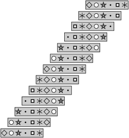
Figure 3. Illustration of multishift coupling for the rectangular distribution. A random point $X$ is drawn from the rectangular distribution with endpoints $L$ and $R$; in the figure six possible such points are denoted by six different symbols. If the square, for instance, is chosen in the first rectangle, then for any other shifted version of the rectangular distribution, the square will be chosen. If a uniformly random symbol/point is drawn from one of the rectangles, then the corresponding symbol/point in any other given fixed rectangle will also be uniformly random.

• Parameters:

• $L=$ left endpoint of rectangle

• $R=$ right endpoint of rectangle

• Random variables:

• $X:=\operatorname{Uniform}(L,R)$

• Mapping:

• $\displaystyle f_{L,R,X}(s)=\left\lfloor\frac{s+R-X}{R-L}\right\rfloor(R-L)+X$

Since $(R-X)/(R-L)$ is uniformly distributed between $0$ and $1$, for any fixed $s$, the fractional part of $(s+R-X)/(R-L)$ is uniformly distributed between $0$ and $1$. If we ignored the floor in the definition of $f(s)$, the expression would simplify to $s+R$. If we refrain from ignoring the floor, then a uniformly random quantity between $0$ and $(R-L)$ is subtracted from $s+R$, so that $f(s)$ is uniformly distributed between $s+L$ and $s+R$, as desired.

It is the floor that makes the image of $f_{L,R,X}$ discrete. If we continuously increase $s$ by $R-L$, the value of $f_{L,R,X}(s)$ changes only once. It is also clear that $f_{L,R,X}(s)$ is monotone in $s$.

2.4.2. Normal distribution

Since we already know how to do multishift coupling for the rectangular distribution, to do the normal distribution, we just need to express it as a convex combination of rectangular distributions. If we pick a random rectangle according to a suitable distribution, and then pick a random point within the rectangle, then the result is a normally distributed random variable. What we will do is pick a random rectangle according to the suitable distribution, and then do multishift coupling with the corresponding rectangular distribution.

There is more than one way to express the normal distribution as a convex combination of rectangular distributions, and we illustrate two of these in Figure 4. In the left part of the figure we have stated the region between the $x$-axis and the probability density function of the normal distribution. (We choose not to normalize the density function by $1/(\sqrt{2\pi}\sigma)$, since the method works fine with unnormalized density functions.) It is well known that if we pick a uniformly random point $(X,Y)$ from the region, then $X$ will be distributed according to a normal distribution. In the right part of the picture we have taken the portion of the region lying to the left of the $y$-axis and reflected it vertically about the line $y=1/2$. If the pick a uniformly random point $(X,Y)$ from this modified region, then $X$ will still be distributed according to a normal distribution. We may view each of these regions as being composed of a stack of many very thin horizontal rectangles (or “layers”), as shown in the lower panels of the figure.

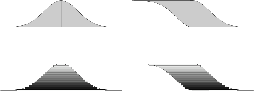
Figure 4. Two different ways of expressing the normal distribution as a convex combination of rectangular distributions. A given rectangle is chosen with probability proportional to its length. The region on the right is obtained by vertically reflecting the left portion of the region on the left.

Let $L$ and $R$ denote the ($x$-coordinates of the) left and right endpoints of the rectangle containing the uniformly random point $(X,Y)$ in the region. If we condition the point $(X,Y)$ to lie within a particular rectangle, then its distribution within the rectangle is uniformly random. In particular, $X$ is uniformly random between $L$ and $R$. If we let $L$ and $R$ specify the random rectangle, and we let $X$ be the uniformly random point from the corresponding rectangular distribution, then since we already know that $X$ is distributed according to a normal distribution, we have our desired decomposition of the normal into a convex combination of rectangular distributions.

We choose to decompose the normal distribution into rectangular distributions using the region on the right of Figure 4 rather than the region on the left, because for the region on the left there is no lower bound on how short the rectangles can get, whereas for the region on the right, there is a positive minimum length for the rectangle.

To pick the point $(X,Y)$ from the region, we draw $X$ from the normal distribution, determine the range of possible values for $Y$, and then pick $Y$ uniformly at random from within this range. To compute $L$ and $R$, we need to be able to invert the probability density function, which we can easily do for the normal distribution. This procedure is re-expressed below.

• Parameters:

• $\sigma=$ standard deviation of normals

• Random variables:

• $X:=\sigma\operatorname{Normal}(0,1)$

• $Y:=\exp(-(X/\sigma)^{2}/2)\operatorname{Uniform}(0,1)$

• If ($X<0$) Then $Y:=1-Y$

• $L:=-\sigma\sqrt{-2\log(1-Y)}$

• $R:=\sigma\sqrt{-2\log(Y)}$

• Mapping:

• $\displaystyle f_{L,R,X}(s)=\left\lfloor\frac{s+R-X}{R-L}\right\rfloor(R-L)+X$

Regarding the efficiency of the coupling, it is clear that either $L$ or $R$ will be at least $\sigma\sqrt{\log 4}$ in absolute value. To show that $R-L\geq\sigma 2\sqrt{\log 4}$, we note

$$w(y)=\sqrt{-2\log y}+\sqrt{-2\log(1-y)}$$

is analytic on $(0,1)$, diverges to infinity as $y\rightarrow 0$ and $y\rightarrow 1$, and show that $w^{\prime}(1/2+t)$ has a real zero only at $t=0$. It follows that $w(1/2)$ minimizes $w$ on $(0,1)$.

$$w^{\prime}(1/2+t)={1/2\over\sqrt{-2\log(1/2+t)}}{-2\over 1/2+t}+ {1/2\over\sqrt{-2\log(1/2-t)}}{2\over 1/2-t}=0$$

$$-2\log(1/2+t)(1/2+t)^{2}= -2\log(1/2-t)(1/2-t)^{2}$$

Since $\log(1/2+t)$ and $(1/2+t)^{2}$ are strictly monotone increasing on $(-1/2,1/2)$, the above equation can have at most one root, which we know must be at $t=0$. Thus the minimum width (normalized to $\sigma$) of any rectangle used in the above procedure is $w(1/2)=2\sqrt{\log 4}$, which is about $2.35482$.

From this it follows that an interval of length $\ell$ is mapped under $f_{L,R,X}$ to at most $\lceil 1+\ell/(2.35\sigma)\rceil$ points.

2.4.3. Multidimensional normal distribution

Extending this approach to the spherically symmetrical multidimensional Gaussian distribution is easy, since the coordinates are independent and are individually Gaussian. Space is divided into rectangular regions, each of which is mapped to a single point. The volume of each rectangular region is at least $(2.35\sigma/\sqrt{d})^{d}$. Thus when the Gaussian is used as a proposal distribution for a Metropolis-Hastings update, and storage is required for each point in the image, even a modest improvement in the constant factor can be significant for large $d$.

2.4.4. Unimodal distributions

The astute reader will have noticed that the only properties about the normal distribution that we used in the coupling procedure of § 2.4.2 are that we can sample from it, it is unimodal (and we know where the mode is), and the probability distribution function $\operatorname{PDF}()$ and its inverse are easy to compute. For other distributions with these properties we can use essentially the same procedure for multishift coupling:

• Random variables:

• $X:=$ RandomSampleFromDistribution()

• $Y:=\operatorname{PDF}(X)*\operatorname{Uniform}(0,1)$

• If ($X<\operatorname{Mode}$) Then $Y:=\operatorname{PDF}(\operatorname{Mode})-Y$

• $L:=\operatorname{LeftInversePDF}(\operatorname{PDF}(\operatorname{Mode})-Y)$

• $R:=\operatorname{RightInversePDF}(Y)$

• Mapping:

• $\displaystyle f_{L,R,X}(s)=\left\lfloor\frac{s+R-X}{R-L}\right\rfloor(R-L)+X$

If the probability distribution has a density function $\operatorname{PDF}()$ with a single mode, then the inverse PDF to the left of the mode is well-defined, and similarly to the right of the mode. This does not necessarily mean that we can compute these inverses effectively (cf. § 2.4.8), but in a certain abstract sense it means that layered multishift can be applied to any unimodal distribution.

Unless the entire distribution is to one side of the mode (which happens in § 2.4.7), there will be a positive minimum length for the rectangles. Thus not only will the image of a finite interval have finite expected size, but the image size will be deterministically bounded.

The alternative generalization (given below) to unimodal distributions is also noteworthy, in that it provides a “maximal coupling”: for any two $s_{1}$ and $s_{2}$, the probability that $f_{L,R,X}(s_{1})=f_{L,R,X}(s_{2})$ is at least as large as it would be for any other coupling of the two distributions.

• Random variables:

• $X:=$ RandomSampleFromDistribution()

• $Y:=\operatorname{PDF}(X)*\operatorname{Uniform}(0,1)$

• $L:=\operatorname{LeftInversePDF}(Y)$

• $R:=\operatorname{RightInversePDF}(Y)$

• Mapping:

• $\displaystyle f_{L,R,X}(s)=\left\lfloor\frac{s+R-X}{R-L}\right\rfloor(R-L)+X$

2.4.5. Multimodal distributions

Even more generally, suppose that the probability density function has multiple modes, and let us assume that the PDF is well-behaved (e.g. almost everwhere differentiable). We don’t give pseudocode for this case, but it is easy to describe in words. Refer back to Figure 4, and recall that we did a vertical reflection to one side of the mode. For multimodal distributions, one could simply reflect the region at each place where the derivitive changes sign, and proceed as before.

2.4.6. Expected image size

We start by computing the expected image size of an interval when the layered multishift coupler is applied to a unimodal distribution. The same formula will hold whether or not we vertically reflect the region on the PDF at its mode. Suppose that a rectangle with endpoints $L$ and $R$ is selected, let $W=R-L$ denote its width. Then conditional on this rectangle being selected, the expected image size of an interval of length $\ell$ is $1+\ell/W$. Thus the (unconditional) expected image size is $1+\ell E[1/W]$. Let $y$ be the vertical coordinate of a thin rectangle with length $W$. The probability that this rectangle is selected is $Wdy$. Thus

$$E[1/W]=\int_{y=0}^{y=y_{\max}}[1/W]Wdy=y_{\max}$$

where $y_{\max}=\operatorname{PDF}(\operatorname{Mode})$ is the height of the distribution at its mode. For instance, using either of our multishift couplers for the normal distribution, an interval of length $\ell$ is mapped under $f_{L,R,X}$ to on average $1+\ell/[\sqrt{2\pi}\sigma]\doteq 1+\ell/(2.5066\sigma)$ points.

In the case of multimodal distributions, if we reflect the region under the PDF each time the derivitive changes sign, then the same reasoning used above still works, except that now

$$y_{\max}=\sum_{\text{local maxima $x$}}\operatorname{PDF}(x)-\sum_{\text{local minima $x$}}\operatorname{PDF}(x).$$

Remark: If instead of measuring expected image size of $f()$, we measured the expected number of times that $f(x)$ changes as $x$ increases, then for unimodal distributions the layered multishift coupler is optimal in that it minimizes the expected number of changes in $f(x)$. Consequently the layered multishift coupler (for unimodal distributions) also has smallest expected image size among the class of monotone multishift couplers.

2.4.7. Exponential distribution

Macro-expanding the generic unimodal procedure we get

• Parameters:

• $\mu=$ mean of exponential

• Random variables:

• $X:=\mu\operatorname{Exponential}(1)$

• $Y:=\exp(-X/\mu)\operatorname{Uniform}(0,1)$

• $L:=0$

• $R:=\mu(-\log(Y))$

• Mapping:

• $\displaystyle f_{L,R,X}(s)=\left\lfloor\frac{s+R-X}{R-L}\right\rfloor(R-L)+X$

which we can simplify to

• Parameters:

• $\mu=$ mean of exponential

• Random variables:

• $X_{1}:=\mu\operatorname{Exponential}(1)$

• $X_{2}:=\mu\operatorname{Exponential}(1)$

• Mapping:

• $\displaystyle f_{X_{1},X_{2}}(s)=\left\lfloor\frac{s+X_{2}}{X_{1}+X_{2}}\right\rfloor(X_{1}+X_{2})+X_{1}$

In § 2.4.8 we will use the observation that if we subtract $X_{2}$ rather than add $X_{1}$, then $f(s)$ will be distributed as $s-$ (rather than $+$) an exponential with mean $\mu$.

Since the entire exponential distribution is to the right of its mode, we no longer have a deterministic upper bound on the size of the image of a finite interval. But from § 2.4.6 we see that the image of an interval of length $\ell$ will have expected size $1+\ell/\mu<\infty$. We remark that this expected image size is equal to that of the Poisson multishift coupler used by Lund and Wilson (1997).

2.4.8. Scaled gamma distribution

Rather than ask that $f(s)$ be distributed as $s+\langle\text{reference distribution}\rangle$, one could instead ask for the distribution to be $s\times\langle\text{reference distribution}\rangle$. This multiscale coupling can of course be reduced to multishift coupling of $\log(f(s))$, so our above techniques can be applied.

One distribution that has been multiscaled in this way (Møller, 1999) is the gamma distribution, which includes as a special case the exponential distribution. Recall that a gamma random variable with shape parameter $\alpha$ and scale parameter 1 has a probability density function given by

$$\operatorname{PDF}(x)=x^{\alpha-1}e^{-x}/\Gamma(\alpha).$$

As mentioned earlier, since Møller (1999) used the coupling $f_{U}(s)=sU$ where $U$ is a gamma random variable, the image of $f_{U}()$ is the continuum.

We could be methodical and specialize the layered multishift coupler for unimodal distributions. Inverting the PDF would require us to solve a transcendental equation, which we would presumably do via Newton’s method. But there is more than one way to decompose a distribution into rectangles. We describe a second method which only uses the standard elementary functions. It is this second method that was used in the timing experiment reported in § 2.3.1.

It is well known (in some circles) that if $G$ is a gamma random variable with shape parameter $\alpha+1$, and $T$ is an independent random variable with exponential distribution and mean $1/\alpha$, then the distribution of $Ge^{-T}$ is a gamma distribution with shape parameter $\alpha$. (The reader unfamiliar with this fact can easily verify it by doing some calculus.) So if we scale $G$ by $e^{\log(s)-T}$ we will get a gamma with the desired shape and scale parameters. Using our above shift coupler for the exponential distribution with negative mean, we get the following procedure

• Parameters:

• $\alpha=$ shape parameter of gamma distribution

• Random variables:

• $G:=\operatorname{Gamma}(\alpha+1,1)$

• $X_{1}:=\operatorname{Exponential}(1)/\alpha$

• $X_{2}:=\operatorname{Exponential}(1)/\alpha$

• Mapping:

• $\displaystyle f_{G,X_{1},X_{2}}(s)=G\exp\left[\left\lfloor\frac{\log(s)+X_{2}}{X_{1}+X_{2}}\right\rfloor(X_{1}+X_{2})-X_{2}\right]$

Once this coupling is written down, it is fairly effortless to use it within a program. Since we are using our earlier shift coupler for the exponential distribution, the number of points in the image of a finite interval will be finite, unbounded, but with finite expectation.

Remark: Since the coupling relies on the multishift coupler for the exponential, one sees that the expected number of points in the image of an interval with aspect ratio $r$ will be $1+\alpha\log r$. If we had instead been methodical and specialized our coupler for unimodal distributions, a few calculations reveal that the expected image size would be $1+[\alpha^{\alpha}e^{-\alpha}/\Gamma(\alpha)]\log r$, or about $1+\sqrt{\alpha/(2\pi)}\log r$ for large $\alpha$.

2.5. Layered multishift coupling ex post facto

One of the hardest parts of using Fill’s algorithm is doing the ex post facto coupling (Murdoch, 1998a). (The reader should read § 1.7 if (s)he has not done so already.) Ex post facto coupling is also required when doing “coupling into and from the past” (§ 1.9.3). So as to facilitate the use of these algorithms when multishift coupling is needed, here we see how to do multishift coupling ex post facto. In fact, the algorithm given by Lund and Wilson (1997) for sampling from the water-level distribution of the infinite dam uses CIAFTP and a multishift coupler for the exponential distribution. As a consequence, in order to substitute the layered multishift coupler, we need to be able to do the layered multishift coupling ex post facto.

Somebody else picks some $s_{0}$, and generates a random variable $X_{0}$ from the given distribution shifted by $s_{0}$. Our job is to generate a random $f()$ such that

• $f(s_{0})=X_{0}$

• When we randomize over the choices of $X_{0}$, the distribution of $f()$ is what it would be if we had simply generated it using the methods in § 2.4.

2.5.1. Unimodal distributions

The appropriate modification of the coupler in § 2.4.4 for unimodal distributions is given below.

• Somebody else does:

• $X_{0}:=s_{0}+$ RandomSampleFromDistribution()

• Random variables we generate:

• $X:=X_{0}-s_{0}$

• $Y:=\operatorname{PDF}(X)*\operatorname{Uniform}(0,1)$

• If ($X<\operatorname{Mode}$) Then $Y:=\operatorname{PDF}(\operatorname{Mode})-Y$

• $L:=\operatorname{LeftInversePDF}(\operatorname{PDF}(\operatorname{Mode})-Y)$

• $R:=\operatorname{RightInversePDF}(Y)$

• Mapping:

• $\displaystyle f_{L,R,X_{0}}(s)=\left\lfloor\frac{s+R-X_{0}}{R-L}\right\rfloor(R-L)+X_{0}$

First note that if $s_{0}=0$ this above modification works: When we randomize over the choices of $X_{0}$ that someone else makes, we just get our previous multishift coupler. Furthermore, since $(R-X)/(R-L)$ is between $0$ and $1$ (and $X=X_{0}$), when we evaluate $f_{L,R,X_{0}}()$ at $s_{0}=0$ we get $X_{0}$, as desired.

If $s_{0}\neq 0$, then we can define $g(s)=f(s_{0}+s)-s_{0}$. When we randomize over $X_{0}$, the statistical properties of $g$ are identical to those of $f$. The condition $f(s_{0})=X_{0}$ translates to $g(0)=X$, so we can do the ex post facto coupling with $g$. Then we translate back in terms of $f$ by $f(s)=g(s-s_{0})+s_{0}$, which simplifies to the above stated formula.

2.5.2. Scaled gamma distribution

In § 2.4.8 we gave an ad hoc layered multiscale coupler for the gamma distribution, which had the virtue of not requiring the ability to compute the inverse probability distribution function. For completeness we describe here how to do this coupling ex post facto.

• Somebody else does:

• $G^{*}:=s_{0}\times\operatorname{Gamma}(\alpha,1)$

• Random variables we generate:

• $G_{\alpha}:=G^{*}/s_{0}$

• $X:=\operatorname{Exponential}(1)$

• $G_{\alpha+1}:=G_{\alpha}+X$

• $X_{2}:=\log(1+X/G_{\alpha})$

• $X_{1}:=\operatorname{Exponential}(1)/\alpha$

• Mapping:

• $\displaystyle\begin{aligned} f_{s_{0},G^{*},X_{1},X_{2}}(s)&=G^{*}\exp\left[\left\lfloor\frac{\log(s/s_{0})+X_{2}}{X_{1}+X_{2}}\right\rfloor(X_{1}+X_{2})\right]\\ &=G_{\alpha+1}s_{0}\exp\left[\left\lfloor\frac{\log(s/s_{0})+X_{2}}{X_{1}+X_{2}}\right\rfloor(X_{1}+X_{2})-X_{2}\right]\end{aligned}$

The key observation is that $G_{\alpha+1}$ and $X_{2}$ are independent of one another, and that $G_{\alpha+1}$ is gamma variate with shape parameter $\alpha+1$ and $X_{2}$ is an exponential variate with mean $1/\alpha$. This we leave as a (perhaps nontrivial) exercise to the reader. Once this observation is verified, the rest should by now be routine.

2.6. Possible extensions

Duncan Murdoch (1998b) has suggested an extension of the layered multishift coupler, which instead of coupling together normals with different means, couples together normals with both different means and different variances.

It is natural to investigate how one might couple together other multiparameter families of distributions. For instance, if one wanted to do simulations of what physicists would call a “$\phi^{4}$ theory”, then rather than couple together normally distributed random variables with different means, one would want to couple together random variables whose unnormalized densities are of the form $\exp(-x^{4}+ax^{3}+bx^{2}+cx)$, and couple these for the various values of $a$, $b$, and $c$. In other words, we’d like to create a random function $f(a,b,c)$ so that the image of $f()$ is discrete, but such that for each fixed $a,b,c$, the random value $f(a,b,c)$ has the appropriate distribution.

3. Perfect Sampling of Autonormal Distributions

3.1. Background

3.1.1. Applications in statistics and physics

The autonormal is an important distribution that arises in both statistics and physics. We quote from lecture notes written by Julian Besag:

The conditional autoregressive or auto–Normal formulation was proposed in Besag (1974, 1975), though it stems from the stationary infinite lattice autoregressions of Lévy (1948) and Rosanov (1967). Gaussian autoregressions have been used in a wide range of applications, including human geography (e.g. Cliff and Ord, 1975, 1981, Ch. 4), agricultural field experiments (e.g. Bartlett, 1978; Kempton and Howes, 1981; Martin, 1990; Cressie and Hartfield, 1993), geographical epidemiology (e.g. Clayton and Kaldor, 1987; Marshall, 1991; Mollié and Richardson, 1991; Bernardinelli and Montomoli, 1992; Cressie, 1993, Ch. 7), astronomy (e.g. Molina and Ripley, 1989; Ripley, 1991), texture analysis (e.g. Chellappa and Kashyap, 1985; Cohen et al., 1991; Cohen and Patel, 1991), and other forms of imaging (e.g. Chellappa, 1985; Jinchi and Chellappa, 1986; Cohen and Cooper, 1987; Simonchy et al., 1989; Zerubia and Chellappa, 1989). Generalizations to multivariate $X_{i}$’s are considered by Kittler and Föglein (1984) and by Mardia (1988), in the context of remote sensing.

In physics the autonormal distribution is called a “free field”, or more precisely, a “discrete free field”. Certain statistical mechanical models (such as the 2D Ising model) have limiting behaviors, in the limit of large system sizes, that are described by free fields. See (Spencer, 1997) for background on free fields in physics.

3.1.2. Definition

A (discrete) free field is a (autonormal) distribution on $n$ random “height” variables $x_{1},\ldots,x_{n}$, with interaction strength $F_{i,j}\geq 0$ between variables $x_{i}$ and $x_{j}$. (In general some of the interaction strengths may be negative, and under suitable conditions the distribution will still be well-defined. We assume in § 3.3 non-negative interaction strengths; this is the principal case of interest in physics.) The values of the heights are well-defined up to a global additive constant, so we arbitrarily pick one of the heights and set its value to be zero. The heights $x_{i}$ and $x_{j}$ act like they’re bound together by a spring with spring-constant $F_{i,j}$, so that the force pulling $x_{i}$ and $x_{j}$ together is $F_{i,j}|x_{i}-x_{j}|$, and the energy in the spring is $\frac{1}{2}F_{i,j}(x_{i}-x_{j})^{2}$. The total energy of the system is then

$$E=\sum_{i<j}\frac{1}{2}F_{i,j}(x_{i}-x_{j})^{2}.$$

The probability distribution is (relative to Lebesgue measure) proportional to $e^{-E}$.

The interaction graph on the sites has an edge between two sites $i$ and $j$ if $F_{i,j}\neq 0$. We will assume that the interaction graph contains a spanning tree, since otherwise the system would break apart into disjoint non-interacting subsystems, which can be dealt with separately.

The simplest example occurs when $n=2$, where $x_{2}-x_{1}$ is distributed as a normal random variable with mean $0$ and variance $1/F_{1,2}$.

Figure 5 shows a random autonormal / free field configuration where the nonzero springs form a regular 2D grid on the torus.

Figure 5. Random free field configuration, with shades of gray representing the height variables. The interaction graph is the regular $50\times 50$ toroidal grid, and the upper-left-most height is tied to $0$. This free field is “massless”; a massive free field would have an extra vertex connected to every site on the grid.

The reason it’s called a free field (as opposed to another kind of field) is that the springs are ideal, i.e. that the force restoring a value to its mean is linear in the displacement, without higher order terms.

3.1.3. Gibbs sampling

Consider the Gibbs-sampling algorithm (single site heat bath). When the heights at all sites other than site $i$ are fixed, the total energy is the following quadratic polynomial in $x_{i}$:

$$\sum_{j}\frac{1}{2}F_{i,j}(x_{i}-x_{j})^{2}+\sum_{i\neq j<k\neq i}\frac{1}{2}F_{j,k}(x_{j}-x_{k})^{2}.$$

The energy is minized when

$$\sum_{j}F_{i,j}(x_{i}-x_{j})=0,\text{\ \ \ \ i.e.\ when\ \ }x_{i}=\sum_{j}x_{j}F_{i,j}/\sum_{j}F_{i,j},$$

and the coefficient of $x_{i}^{2}$ is $\frac{1}{2}\sum_{j}F_{i,j}$. Thus the conditional distribution of the height $x_{i}$ given the remaining heights is governed by a normal distribution with mean

$$\sum_{j}x_{j}F_{i,j}/\sum_{j}F_{i,j},$$

and variance

$$1/\sum_{j}F_{i,j}.$$

Equivalently, the height $x_{i}$ acts as if a spring with spring constant $\sum_{j}F_{i,j}$ is pulling it to a weighted average of the neighboring heights. Recall that the Gibbs sampler visits the sites, either in sequence or at random, and randomizes the height $x_{i}$ at a visited site $i$ by drawing it from the conditional distribution given the remaining heights. The term “autonormal” comes from that fact that each variable is normally distributed with nonrandom variance and mean determined by a weighted average of its neighbors.

3.1.4. Linear algebra methods

If the matrix of interaction strengths $F_{i,j}$ can be diagonalized into an orthonormal basis of eigenvectors $\vec{v}_{1},\ldots,\vec{v}_{n}$ with eigenvalues $\lambda_{1},\ldots,\lambda_{n}$, then a random sample can be generated by

$$\sum_{i:\lambda_{i}\neq 0}\frac{\operatorname{Normal}(0,1)}{\sqrt{\lambda_{i}}}\vec{v}_{i},$$

where the Gaussian random variables in the sum are independent of one another. If the interaction graph is a regular lattice, then this approach becomes particularly effective as FFTs can be used (see e.g. (Dietrich and Newsam, 1997)). If the interaction strengths are nonuniform or the graph is irregular, then the linear algebra becomes more complicated, and practitioners often prefer the simplicity offered by Markov chain approaches (Besag, 1998).

3.2. Using multishift coupling

An important property of the layered multishift couplers is that they are all monotone couplings. What this means is that if somehow we can get an upper bound and lower bound on the values of each variable, $\ell_{i}\leq x_{i}\leq u_{i}$ for each i, then we can repeatedly update the lower configuration ($x_{i}=\ell_{i}$ for each $i$) and upper configuration ($x_{i}=u_{i}$ for each $i$) using Gibbsian updates with the layered multishift coupler for the normal (§ 2.4.2). When the upper and lower configurations get mapped to the same value, every other possible configuration also gets mapped to this value. Because we are using a multishift coupler that maps reasonably large segments of the reals to the same point, the upper and lower configurations will in fact (with probability $1$) eventually converge to exactly the same value. Pseudocode for this approach is given in Figure 6.

• $T:=1$    /* Start at time $-1$ in the past */

• Repeat {

• /* Set := truncated $\langle\text{state space}\rangle$*/

• $\ell_{1}:=0;u_{1}:=0$    /* First site is tied to 0 */

• For $i:=2$ to  $n$

• $\ell_{i}:=-10^{6}$; $u_{i}:=10^{6}$    /* (plausible assumption) */

• For $t$ := $T$ DownTo $1$ {     /* Proceed to time zero */

• /* Take care to use previously used random coins */

• If $t$ is a power of 2

• SetRandomSeed(seed[$i$,$\log_{2}(t)$])

• /* ApplyRandomMap(Set) */

• For $i:=2$ To $n$ /* randomize each site (except the one tied to 0) */

• /* Apply the multishift coupler for the normal at site $i$ */

• /* First pick the parameters defining $f_{L,R,X}()$ at site $i$ */

• $\sigma:=\sum_{j}F_{i,j}$

• $X:=\sigma\operatorname{Normal}(0,1)$

• $Y:=\exp(-(X/\sigma)^{2}/2)\operatorname{Uniform}(0,1)$

• If ($X<0$) Then $Y:=1-Y$

• $L:=-\sigma\sqrt{-2\log(1-Y)}$

• $R:=\sigma\sqrt{-2\log(Y)}$

• /* Next apply $f_{L,R,X}()$ to the upper and lower bounds */

• $\mu_{\ell}:=\sum_{j}\ell_{j}F_{i,j}/\sum_{j}F_{i,j}$

• $\mu_{u}:=\sum_{j}u_{j}F_{i,j}/\sum_{j}F_{i,j}$

• $\displaystyle\ell_{i}:=f_{L,R,X}(\mu_{\ell})=\left\lfloor\frac{\mu_{\ell}+R-X}{R-L}\right\rfloor(R-L)+X$

• $\displaystyle u_{i}:=f_{L,R,X}(\mu_{u})=\left\lfloor\frac{\mu_{u}+R-X}{R-L}\right\rfloor(R-L)+X$

• }

• /* It’s now time zero, test for coalescence */

• If $u_{i}=\ell_{i}$ for each $i$ then return $[\ell_{1},\ldots,\ell_{n}]$

• $T:=2*T$    /* Otherwise try again starting twice as far in the past */

• }

Figure 6. Pseudocode for generating random samples from an approximation to the autonormal distribution. The basic algorithm is monotone coupling from the past using the Gibbs sampler Markov chain, with $\ell_{i}$ and $u_{i}$ representing lower and upper bounds on the height at site $i$. The multishift coupler for the normal distribution is used when doing updates because (1) it correctly give the normal distribution, (2) it is monotone, and (3) with probability one the upper and lower bounds on the state will eventually be exactly equal. The approximation error (which comes from using $\pm 10^{6}$ in place of $\pm\infty$ in the initial upper and lower bounds on the state) will in practice be minor; in § 3.3 we will see how to eliminate this error altogether.

In the event that some of the interaction strengths $F_{i,j}$ are negative, we can just use a combination of monotone and anti-monotone coupling. In Figure 6, the definitions of $\mu_{\ell}$ and $\mu_{u}$ become

$$\mu_{\ell}:=\frac{\sum_{j:F_{i,j}\geq 0}\ell_{j}F_{i,j}+\sum_{j:F_{i,j}<0}u_{j}F_{i,j}}{\sum_{j}F_{i,j}}$$

and

$$\mu_{u}:=\frac{\sum_{j:F_{i,j}\geq 0}u_{j}F_{i,j}+\sum_{j:F_{i,j}<0}\ell_{j}F_{i,j}}{\sum_{j}F_{i,j}}.$$

Møller (1999) also mentions mixed monotone/anti-monotone coupling.

How do we get these upper and lower bounds? It may be tempting to simply use values such as $10^{6}$ and $-10^{6}$, since only a small portion of the probability distribution is so far out in the tails. If we did truncate the state space, the running time would increase logarithmically in the truncation parameter, while the truncation bias would decrease exponentially. But there are reasons not do this: 1) for strongly coupled systems, using such large values will noticeably and needlessly slow convergence, 2) for weakly coupled systems $10^{6}$ may not be large enough, and 3) it’s theoretically displeasing. In § 3.3 we see how to do without artificial truncations such as this.

3.3. Using Murdoch’s method

At this point the reader should go back and read § 1.9.2 if (s)he has not done so already.

3.3.1. Proposal distribution

There is room for engineering art when picking the proposal distribution for the independence sampler. One reasonable choice for the autonormal is the following. First pick a spanning tree of the graph rooted at the special vertex whose height is zero. We assign the value $x_{v}$ at vertex $v$ only after assigning the value at $v$’s parent $u$ in the tree. The distribution of $x_{v}$ is a normal with mean $x_{u}$ and variance $2/F_{u,v}$. Call the resulting configuration $B$. Let $E_{\operatorname{tree}}(B)$ be the energy contained in just those springs that are part of the spanning tree. The probability density of the proposal distribution (relative to Lebesgue measure) is then $\exp(-E_{\operatorname{tree}}(B)/2)$.

According to the Metropolis-Hastings update rule, when the current state is $A$ and the proposal is $B$, we always accept the proposal $B$ if

$$\pi(A)P_{A}(B)\leq\pi(B)P_{B}(A),$$

where $\pi(x)$ is the desired probability of state $x$ in a discrete space, and $P_{x}(y)$ is the probability of a transition from $x$ to $y$. Otherwise we accept the proposal with some probability less than one. In the continuum limit, for our application the above relation amounts to

$$\exp(-E(A))\exp(-E_{\operatorname{tree}}(B)/2) \leq\exp(-E(B))\exp(-E_{\operatorname{tree}}(A)/2)$$

$$E(A)-E_{\operatorname{tree}}(A)/2 \geq E(B)-E_{\operatorname{tree}}(B)/2$$

$$E(A)+(E(A)-E_{\operatorname{tree}}(A)) \geq 2E(B)-E_{\operatorname{tree}}(B)$$

which holds whenever

$$E(A) \geq E_{\max}\equiv 2E(B)-E_{\operatorname{tree}}(B).$$

Any state $A$ with energy $E(A)\geq E_{\max}$ gets mapped to state $B$. Furthermore, $E(B)\leq E_{\max}$. Therefore, after the Metropolis-Hastings update we are guaranteed that the energy of the updated state is at most $E_{\max}$.

3.3.2. Finite box containing updated state

We again use the spanning tree when converting this bound on the energy to an upper and lower bound on the value of each coordinate. Vertices $v$ adjacent to the distinguished vertex have easy bounds on their values $x_{v}$:

$$|x_{v}|\leq\sqrt{2E_{\max}/F_{v,0}},$$

since if $|x_{v}|$ were any larger, the energy in just the spring connecting $v$ to the distinguished vertex would exceed to total possible energy $E_{\max}$.

To deal with vertices further away from the special vertex, we prove by induction the following claim:

Claim 3.1.

Given vertices $v_{0},\ldots,v_{k}$, where $k>0$, $x_{v_{0}}=0$ and $x_{v_{k}}=x$, if we seek to minimize the energy just in the springs $(v_{0},v_{1}),\ldots,(v_{k-1},v_{k})$, this minimum energy is $\frac{1}{2}[1/(1/F_{1}+\cdots+1/F_{k})]x^{2}$ where $F_{i}$ denotes $F_{v_{i-1},v_{i}}$.

Proof.

This claim hold trivially for $k=1$. Suppose that it holds for $k$, we prove it for $k+1$. Let $x=x_{v_{k+1}}$ and $y=x_{v_{k}}$. By induction the minimum energy contained in the given springs is

$$\frac{1}{2}Fy^{2}+\frac{1}{2}F^{\prime}(y-x)^{2}$$

where we have for convenience let $F$ denote $[1/(1/F_{1}+...+1/F_{k})]$ and $F^{\prime}$ denote $F_{k+1}$. This energy is minimized when

$$Fy+F^{\prime}(y-x) =0$$

$$y =F^{\prime}x/(F+F^{\prime})$$

at which point the energy takes the value

$$E =\frac{1}{2}F\left({F^{\prime}x\over F+F^{\prime}}\right)^{2}+\frac{1}{2}F^{\prime}\left({F^{\prime}x\over F+F^{\prime}}-x\right)^{2}$$

$$=\frac{1}{2}F\left({F^{\prime}x\over F+F^{\prime}}\right)^{2}+\frac{1}{2}F^{\prime}\left({-Fx\over F+F^{\prime}}\right)^{2}$$

$$=\frac{1}{2}\left[{(F{F^{\prime}}^{2}+F^{2}F^{\prime})\over(F+F^{\prime})^{2}}\right]x^{2}$$

$$=\frac{1}{2}\left[{FF^{\prime}\over F+F^{\prime}}\right]x^{2}$$

$$=\frac{1}{2}\left[{1\over 1/F+1/F^{\prime}}\right]x^{2}$$

$$=\frac{1}{2}\left[{1\over(1/F_{1}+\cdots+1/F_{k})+1/F_{k+1}}\right]x^{2}$$

as claimed. ∎

From this we conclude

$$|x_{v_{k}}|\leq\sqrt{2E_{\max}[1/F_{1}+\cdots+1/F_{k}]}.$$

3.4. CFTP using composite random maps

Next we suitably mix the independence sampler and the Gibbsian updates to define a composite Markov chain with which we can do CFTP. We use a mixing strategy different from the one originally advocated by Murdoch (1999), since the strategy below is easier to use for this problem. The composite Markov chain that we use is given by the following update rule:

Input: current state $x$

1. Generate a proposal state for the independence sampler.

2. Ignoring $x$, get upper and lower bounds $u$ and $\ell$ on resulting state that would hold regardless of input.

3. Do Gibbsian updates on $u$ and $\ell$ (but not $x$) with the layered multishift coupler until $u=\ell$. Let $C$ be the number of Gibbsian updates performed.

4. Generate a proposal state for the independence sampler (independent of the previous one).

5. Ignoring $x$, get upper and lower bounds $u$ and $\ell$ on resulting state that would hold regardless of input.

6. With the usual Metropolis-Hastings probability, either set $x$ to the proposal, or leave it unmodified.

7. Do $C$ Gibbsian updates with the layered multishift coupler starting from the states $u$, $\ell$, and $x$.

8. Output state $x$, and declare coalescence if $u=\ell$.

We make a few observations:

1. If we pick a random natural number $C$ from any distribution and then do $C$ updates of a state distributed according to $\pi$, the result will be distributed according to $\pi$. Therefore the above randomizing operation preserves the desired distribution $\pi$.

2. If $u=\ell$, then the output state is independent of the input state.

3. $\Pr[u=\ell]\geq 1/2$.

Now we view these randomizing process as one step of a composite Markov chain with the desired steady-state distribution $\pi$, and do CFTP with the composite randomizing operations. To do CFTP we compose the maps defined by these Markovian updates going back in time. A convenient way to do this is to just keep trying new random maps $F_{-1},F_{-2},\ldots$ until we find a map $F_{-T}$ which by itself is coalescent (as determined by the $u=\ell$ test). The expected value of $T$ is at most $2$. Then we take the image of $F_{-T}$, and determine where the maps $F_{-T+1},\ldots,F_{-1}$ take it to at time $0$.

We remark that we can also use these composite random maps in the read-once version of CFTP described by (Wilson, 1999), and that this is in fact the approach we took when generating the sample shown in Figure 5.

Source code

The programs used to make Figure 5 and the simulation results in § 2.3.1 are available at this article’s web site http://dbwilson.com/shift/.

References

- Aldous (1995) David Aldous. On simulating a Markov chain stationary distribution when transition probabilities are unknown. In David Aldous, Persi Diaconis, Joel Spencer, and J. Michael Steele, editors, Discrete Probability and Algorithms, volume 72 of IMA Volumes in Mathematics and its Applications, pages 1–9. Springer-Verlag, 1995.
- Aldous (1990) David J. Aldous. A random walk construction of uniform spanning trees and uniform labelled trees. SIAM Journal on Discrete Mathematics, 3(4):450–465, 1990.
- Aldous and Fill (199X) David J. Aldous and James A. Fill. Reversible Markov Chains and Random Walks on Graphs. Book in preparation, http://www.stat.berkeley.edu/~aldous/ book.html, 199X.
- Asmussen et al. (1992) Søren Asmussen, Peter W. Glynn, and Hermann Thorisson. Stationary detection in the initial transient problem. ACM Transactions on Modeling and Computer Simulation, 2(2):130–157, 1992.
- Besag (1998) Julian Besag, 1998. Personal communication.
- Besag and Kooperberg (1995) Julian Besag and Charles Kooperberg. On conditional and intrinsic autoregressions. Biometrika, 82(4):733–746, 1995.
- Blöte and Hilhorst (1982) H. W. J. Blöte and H. J. Hilhorst. Roughening transitions and the zero-temperature triangular Ising antiferromagnet. Journal of Physics A, 15(11):L631–L637, 1982.
- Broder (1989) Andrei Broder. Generating random spanning trees. In 30th Annual Symposium on Foundations of Computer Science, pages 442–447, 1989.
- Conway and Lagarias (1990) John Conway and Jeffrey Lagarias. Tiling with polyominoes and combinatorial group theory. Journal of Combinatorial Theory, series A, 53:183–208, 1990.
- Diaconis and Freedman (1999) Persi Diaconis and David Freedman. Iterated random functions. SIAM Review, 41(1):45–76, 1999.
- Dietrich and Newsam (1997) C. R. Dietrich and G. N. Newsam. Fast and exact simulation of stationary Gaussian processes through circulant embedding of the covariance matrix. SIAM Journal on Scientific Computing, 18(4):1088–1107, 1997.
- Dimakos (1999) Xeni K. Dimakos. A guide to exact simulation. International Statistical Review, 1999. To appear.
- Felsner and Wernisch (1997) Stefan Felsner and Lorenz Wernisch. Markov chains for linear extensions, the two-dimensional case. In Proceedings of the Eighth Annual ACM-SIAM Symposium on Discrete Algorithms, pages 239–247, 1997.
- Fill and Machida (1998) James A. Fill and Motoya Machida. Stochastic monotonicity and realizable monotonicity. Technical Report 573, Department of Mathematical Sciences, The Johns Hopkins University, 1998.
- Fill (1998a) James Allen Fill. An interruptible algorithm for perfect sampling via Markov chains. The Annals of Applied Probability, 8(1):131–162, 1998a.
- Fill (1998b) James Allen Fill. The move-to-front rule: A case study for two exact sampling algorithms. Probability in the Engineering and Informational Sciences, 12:283–302, 1998b.
- Fill et al. (1999) James Allen Fill, Motoya Machida, Duncan J. Murdoch, and Jeffrey S. Rosenthal. Extension of Fill’s perfect rejection sampling algorithm to general chains, 1999. Preprint.
- Fortuin and Kasteleyn (1972) C. M. Fortuin and P. W. Kasteleyn. On the random cluster model. I. Introduction and relation to other models. Physica, 57(4):536–564, 1972.
- Foss (1996) S. G. Foss, 1996. Personal communication.
- Gelfand and Smith (1990) A. E. Gelfand and A. F. M. Smith. Sampling-based approaches to calculating marginal densities. Journal of the American Statistical Association, 85:398–409, 1990.
- Glynn and Heidelberger (1990) Peter W. Glynn and Philip Heidelberger. Bias properties of budget constrained simulations. Operations Research, 38(5):801–814, 1990.
- Goldberg (1990) David Goldberg. Computer Arithmetic. Appendix A of Computer Architecture: A Quantitative Approach, by David A. Patterson and John L. Hennessy. Morgan Kaufmann Publishers, 1990.
- Green and Murdoch (1999) Peter J. Green and Duncan J. Murdoch. Exact sampling for Bayesian inference: towards general purpose algorithms (with discussion). In J. M. Bernardo, J. O. Berger, A. P. Dawid, and A. F. M. Smith, editors, Bayesian Statistics 6, pages 301–321. Oxford University Press, 1999. Presented as an invited paper at the 6th Valencia International Meeting on Bayesian Statistics, Alcossebre, Spain, June 1998.
- Häggström et al. (1999) O. Häggström, M. N. M. van Lieshout, and J. Møller. Characterisation results and Markov chain Monte Carlo algorithms including exact simulation for some spatial point processes. Bernoulli, 5:641–658, 1999.