The Homotopy Classification and the Index of Boundary Value Problems for General Elliptic Operators

Abstract

We give the homotopy classification and compute the index of boundary value problems for elliptic equations. The classical case of operators that satisfy the Atiyah–Bott condition is studied first. We also consider the general case of boundary value problems for operators that do not necessarily satisfy the Atiyah–Bott condition.

Keywords: elliptic boundary value problems, Atiyah–Bott condition, index theory, $K$-theory, homotopy classification

1991 AMS classification: Primary 58G20, Secondary 58G10, 19M05, 35J55

Introduction

The present paper deals with the theory of boundary value problems for elliptic equations. The well-known Shapiro–Lopatinskii condition (e.g., see [1]) describes the class of elliptic boundary value problems, i.e., problems defining Fredholm operators in Sobolev spaces. On the other hand, this condition represents the obstruction to the existence of well-posed (Fredholm) boundary value problems for elliptic operators on manifolds with boundary. Moreover, from the topological point of view, the Shapiro–Lopatinskii condition guarantees the existence of a homotopy of the homogeneous principal symbol of the given elliptic operator to a symbol independent of the cotangent variables in a neighborhood of the boundary. This restatement of the Shapiro–Lopatinskii condition was found by Atiyah and Bott [2] and is often called the Atiyah–Bott condition. From the analytical point of view, the Shapiro–Lopatinskii condition permits one to reduce a boundary value problem to a zero-order elliptic operator that is a bundle homomorphism in a neighborhood of the boundary. A reduction of this kind is fundamental for the homotopy classification of elliptic boundary value problems and for the derivation of the corresponding index formula.

As was already pointed out, not all operators on a manifold with boundary admit well-posed classical boundary value problems. The theory of boundary value problems for general elliptic operators (which need not satisfy the Atiyah–Bott condition) was constructed in [3]. In this theory, the violation of the Shapiro–Lopatinskii–Atiyah–Bott condition does not allow one to reduce an elliptic boundary value problem to a zero-order operator. Nonetheless, the reduction is possible if the boundary value problem possesses certain symmetries. In this case, it is also possible to give a homotopy classification of elliptic boundary value problems with symmetries and obtain an index formula.

Let us describe the contents of the paper in more detail.

The first part of the paper deals with classical boundary value problems. The main result here is the homotopy classification of boundary value problems. More precisely, it is shown that a boundary value problem satisfying the Shapiro–Lopatinskii condition admits a reduction to a zero-order operator that requires no boundary conditions, i.e., there is an isomorphism

$$\varepsilon_{m}:{\rm\mathop{Ell}}^{m}\left(M\right)\longrightarrow{\rm\mathop{Ell}}^{0}\left(M\right)$$

of the group of stably homotopic elliptic boundary value problems for operators of order $m\geq 1$ and a similar group for zero-order operators. Furthermore, the operators of order zero are classified, in the same way as in elliptic theory on closed manifolds, by their principal symbols

$$\chi:{\rm\mathop{Ell}}^{0}\left(M\right)\longrightarrow K\left(T^{*}\left(M\backslash\partial M\right)\right),$$

where $K\left(T^{*}\left(M\backslash\partial M\right)\right)$ is the $K$-group with compact supports. In this section of the paper we follow Hörmander [1], who realized the topological method due to Atiyah–Bott [2] by explicit homotopies of boundary value problems. We point out that Hörmander’s homotopies of classical boundary value problems do not use the complete Boutet de Monvel algebra [5]. This permits one to obtain the homotopy classification of boundary value problems and the corresponding index formula and simultaneously prove the Atiyah–Bott theorem on the obstruction to the existence of classical boundary value problems.

In the second part of the paper, we consider boundary value problems [3] for operators that do not satisfy the Shapiro–Lopatinskii–Atiyah–Bott condition. These boundary value problems have the form

$$\left\{\begin{array}[]{ll}Du=f,&u\in H^{s}\left(M,E\right),\quad f\in H^{s-m}\left(M,F\right),\vspace{0.2cm}\\ Bj_{\partial M}^{m-1}u=g,&g\in{\rm Im}\,P\subset H^{\sigma}\left(\partial M,G\right),\end{array}\right.$$ (1)

where $B$ is a boundary operator with range contained in the range ${\rm Im}\,P$ of a pseudodifferential projection $P$ in the Sobolev space on the boundary of $M$ and $j_{\partial M}^{m-1}$ is the composition of the jet of order $m-1$ and the restriction to the boundary $\partial M$. In view of the Atiyah–Bott obstruction, the boundary value problem (14) cannot be reduced to an operator of order zero. However, an arbitrary elliptic boundary value problem can be reduced in this case to the so-called spectral boundary value problem [6, 7] for a first-order operator.

Further simplification of the boundary value problem is possible under additional assumptions on the subspace defined by the pseudodifferential projection on the right-hand side in (1). An example of such assumptions is given by parity conditions imposed on the principal symbol of the projection (see [8, 9]). Precise definitions will be given below, and for now we only mention that these conditions can be reformulated as conditions under which the operator $D$ of the boundary value problem extends to the double of the manifold with boundary in a symmetric way. This restatement shows that the parity condition is a generalization of the Atiyah–Bott condition, which guarantees the existence of a homotopy of the principal symbol of the operator to the identity symbol in a neighborhood of the boundary (and, of course, the possibility of extension to the double).

Under the above-mentioned parity conditions, the stable homotopy classification modulo 2-torsion is obtained for elliptic boundary value problems. It has the form

$${\rm\mathop{Ell}}^{ev/odd}\left(M,\partial M\right)\otimes{\bf Z}\left[\frac{1}{2}\right]\simeq K\left(T^{*}\left(M\backslash\partial M\right)\right)\otimes{\bf Z}\left[\frac{1}{2}\right]\oplus{\bf Z}\left[\frac{1}{2}\right],$$ (2)

where the first term in the sum is determined by the principal symbol of the boundary value problem and the second component is given by the value of a functional $d$ on the set of subspaces defined by pseudodifferential projections (this functional was defined in [8, 9]). The functional $d$ is equal to the Atiyah–Patodi–Singer spectral $\eta$-invariant [6] of an admissible self-adjoint operator for the case in which the subspace in question is the nonnegative spectral subspace of that operator [10, 8].

The index formula for boundary value problems with parity conditions [8, 9] readily follows from the homotopy classification (2) in a natural way.

The authors are grateful to V. E. Nazaikinskii for numerous useful discussions. The results of the paper were reported at the international conference ”Workshop in Partial Differential Equations,” July 1999, Potsdam, Germany and also at the conference ”Jean Leray 1999,” August 1999, Karlskrona-Ronneby, Sweden.

1 Classical boundary value problems

1.1 Basic definitions

Let $M$ be a compact smooth manifold with boundary $X=\partial M$ and

$$D:H^{s}\left(M,E\right)\longrightarrow H^{s-m}\left(M,F\right)$$

an elliptic differential operator of order $m\geq 1$ acting in Sobolev spaces of sections of vector bundles $E,F$ over $M$. The operator $D$ is not Fredholm, since its kernel $\ker D$ is infinite-dimensional. To define a Fredholm operator, let us equip $D$ with some boundary conditions. To this end, we choose a collar neighborhood $U=X\times\left[0,1\right)\subset M$ of $X$ with normal coordinate $t\in\left[0,1\right)$. Consider jets of order $m-1$ in the normal direction to the boundary composed with the operator of restriction to the boundary

$$\begin{array}[]{c}j_{X}^{m-1}u=\left(\left.u\right|_{X},\left.-i\frac{\partial}{\partial t}u\right|_{X},\ldots,\left.\left(-i\frac{\partial}{\partial t}\right)^{m-1}u\right|_{X}\right),\\ j_{X}^{m-1}:H^{s}\left(M,E\right)\rightarrow\bigoplus_{k=0}^{m-1}H^{s-1/2-k}\left(X,\left.E\right|_{X}\right).\end{array}$$

A classical boundary value problem for $D$ is a system of equations of the form

$$\left\{\begin{array}[]{ll}Du=f,&u\in H^{s}\left(M,E\right),f\in H^{s-m}\left(M,F\right),\vspace{0.2cm}\\ Bj_{X}^{m-1}u=g,&g\in H^{\sigma}\left(X,G\right),\end{array}\right.$$ (3)

where

$$B:\bigoplus_{k=0}^{m-1}H^{s-1/2-k}\left(X,\left.E\right|_{X}\right)\longrightarrow H^{\sigma}\left(X,G\right)$$ (4)

is a pseudodifferential operator on the boundary; the orders of its components and the indices of Sobolev spaces in (4) are supposed to be compatible in a natural way (e.g., see [1]). For brevity, the boundary value problem $\left(D,B\right)$ will sometimes be denoted by ${\cal D}.$

On the cotangent sphere bundle $S^{*}X$ of $X$, we consider the vector bundle

$$L_{+}\left(D\right)\subset\pi^{*}E^{m},\qquad\pi:S^{*}X\rightarrow X,$$

whose fiber over a point $(x,\xi)\in S^{*}X$ is the subspace of initial data of bounded solutions of the ordinary differential equation

$$\sigma\left(D\right)\left(x,0,\xi^{\prime},-i\frac{d}{dt}\right)u\left(t\right)=0,\qquad\left(x,\xi^{\prime}\right)\in S^{*}X,$$

with constant coefficients on the half-line $\left\{t\geq 0\right\}$. The complementary subbundle corresponding to solutions bounded as $t\rightarrow-\infty$ is denoted by $L_{-}\left(D\right)$. The subbundles $L_{\pm}\left(D\right)$ are obviously determined by the restriction of the principal symbol of $D$ to the boundary.

The restriction

$$L_{+}\left(D\right)\stackrel{{\scriptstyle\sigma\left(B\right)}}{{\longrightarrow}}\pi^{*}G$$ (5)

of the principal symbol of the boundary operator $B$ to the subbundle $L_{+}\left(D\right)\subset\pi^{*}E^{m}$ is called the boundary symbol of classical boundary value problem $\left(D,B\right)$.

The boundary value problem $\left(D,B\right)$ is said to be elliptic if its boundary symbol is an isomorphism of vector bundles.

Proposition 1

(e.g., see [1]) The boundary value problem (3) has the Fredholm property if and only if it is elliptic.

The ellipticity condition (5) imposes an essential restriction on the bundle $L_{+}\left(D\right)$: for the existence of an elliptic boundary value problem for $D$, it is necessary that this bundle be isomorphic to a bundle lifted from $X$; the choice of a specific lifting (5) determines the boundary conditions. Atiyah and Bott [2] noted that this condition can be restated in terms of the principal symbol of $D$ in the following form: the restriction of $\sigma\left(D\right)$ to $X$ is stably homotopic to the symbol of a multiplication operator, that is,

$$\sigma\left(D\right)\left(x,0,\xi\right)\sim\sigma^{\prime}\left(x\right),$$ (6)

or, in terms of $K$-theory,

$$\left[\sigma\left(D\right)\right]\in{\rm Im}\,\left\{K\left(T^{*}\left(M\backslash\partial M\right)\right)\stackrel{{\scriptstyle\pi^{*}}}{{\longrightarrow}}K\left(T^{*}M\right)\right\},\quad\pi:T^{*}M\rightarrow\left.T^{*}M\right/\left.T^{*}M\right|_{X}.$$

Furthermore, the choice of a boundary condition determines a certain homotopy of the form (6), which specifies an element

$$\left[\sigma\left(D,B\right)\right]\in K\left(T^{*}\left(M\backslash\partial M\right)\right).$$

It turns out (see Section 2) that this element classifies the boundary value problem $\left(D,B\right)$ up to stable homotopy equivalence.

In the next section, we carry out the homotopy classification of elliptic boundary value problems. To this end, we have to enlarge the class of operators for which boundary value problems will be posed. Namely, we deal with elliptic operators $D$ on a manifold $M$ with boundary $X$ which satisfy the following conditions.

1. In a small neighborhood $X\times\left[0,2\varepsilon\right)$ of the boundary, $D$ has the form

   $$D=\sum_{k=0}^{m}D_{k}\left(t\right)\left(-i\frac{\partial}{\partial t}\right)^{m-k},$$ (7)

   where the $\!D_{k}\!\left(t\right)$ are smooth families of pseudodifferential operators on $\!X\!$, ${\rm\mathop{ord}}D_{k}\!\left(t\right)\!=k,$ such that $D_{0}\left(t\right)$ consists of isomorphisms of vector bundles. By identifying the vector bundles in which $D$ acts with the help of this isomorphism in a neighborhood of the boundary, we can assume that the coefficient $D_{0}\left(t\right)$ is the identity operator;

2. Outside the collar neighborhood $X\times\left[0,1\right)$ of the boundary, $D$ is a pseudodifferential operator of order $m$;

3. In the domain $X\times\left(\varepsilon,1\right)$, $D$ is a pseudodifferential operator with continuous symbol (see [11] or [12, 1]).

For this class of operators, boundary value problems can be posed in the same way as above. The definition of the subbundles $L_{\pm}\left(D\right)$ and the ellipticity condition remain valid.

1.2 Example

Let us consider an example of a boundary value problem for operators of the form (7).

On a manifold $M$, we consider a bundle $E$ and a decomposition of this bundle in a neighborhood of the boundary $X$ into the sum of two subbundles

$$\left.E\right|_{U_{X}}=E_{+}\oplus E_{-}.$$ (8)

For the bundles $\left.E_{\pm}\right|_{X}$, let us take elliptic first-order operators $\Lambda_{\pm}$ with principal symbol $\left|\xi^{\prime}\right|.$ We also choose a first-order operator $\Lambda_{M}$ on $M$ with principal symbol $\left|\xi\right|$ which acts in the bundle $E$. In accordance with the decomposition (8), let us consider the following first-order elliptic operator in a neighborhood of the boundary:

$$D_{\pm}=\left(-i\frac{\partial}{\partial t}+i\Lambda_{+}\right)\oplus\left(i\frac{\partial}{\partial t}+i\Lambda_{-}\right):C^{\infty}\left(U_{X},E\right)\rightarrow C^{\infty}\left(U_{X},E\right).$$ (9)

The relation 

$$L_{+}\left(D_{\pm}\right)=0\oplus\pi^{*}E_{-},\qquad\pi:S^{*}X\rightarrow X,$$

shows that the boundary condition

$$\left.u_{-}\right|_{X}=g\in C^{\infty}(X,E_{-})\qquad{\mbox{{\em for} }}u=\left(u_{+},u_{-}\right)\in C^{\infty}\left(U_{X},E_{+}\oplus E_{-}\right)$$ (10)

defines an elliptic boundary value problem for the operator (9). Let us extend $D_{\pm}$ to the interior of the manifold. Consider a cutoff function $\chi$ on $M$, $0\leq\chi\left(t\right)\leq 1,$that is equal to $1$ for $0\leq t\leq 1/3$ and is zero for $t\geq 2/3.$ The desired extension of the operator is given by the formula

$$D_{\pm}=\chi\left(t\right)\left[\left(-i\frac{\partial}{\partial t}+i\Lambda_{+}\right)\oplus\left(i\frac{\partial}{\partial t}+i\Lambda_{-}\right)\right]+\left(1-\chi\left(t\right)\right)i\Lambda_{M}.$$ (11)

The boundary value problem for the operator $D_{\pm}$ with the boundary condition (10) is denoted by ${\cal D}_{\pm}$. It is well-known (e.g., see [1] or [5]) that this boundary value problem has index zero. This follows, for example, from the observation that the family of boundary value problems

$${\cal D}_{\pm}+ip$$

is an elliptic family in the half-plane ${\rm Re}\,p>0$ in the sense of Agranovich–Vishik [13]. Consequently, it is invertible for sufficiently large values of the parameter $p.$The invertibility of the family ${\cal D}_{\pm}+ip$ can be shown directly (see [1]).

If one of the bundles $E_{\pm}$ coincides with the entire $E,$ then the corresponding operator $D_{\pm}$ is denoted by $D_{-}$ or $D_{+}.$ For example, the operator $D_{+}$ does not contain boundary conditions.

2 The  homotopy  classification  of  boundary  value problems

2.1 Classification of operators of order zero

In the class of elliptic operators on manifolds with boundary introduced in the end of the previous section, operators of order zero play an important role, since these operators do not require boundary conditions.

The abelian group of stable homotopy classes of elliptic zero-order operators is denoted by ${\rm\mathop{Ell}}^{0}\left(M\right)$.

An elliptic operator $D$ of order zero is a bundle isomorphism in a neighborhood of the boundary of $M$ (see (7)); hence, its principal symbol defines an element of $K$-theory with compact supports:

$$\left[\sigma\left(D\right)\right]\in K\left(T^{*}\left(M\backslash\partial M\right)\right).$$

Thus, we have the homomorphism

$$\begin{array}[]{ccc}\chi:{\rm\mathop{Ell}}^{0}\left(M\right)&\longrightarrow&K\left(T^{*}\left(M\backslash\partial M\right)\right),\\ &&\\ \left[D\right]&\mapsto&\ \left[\sigma\left(D\right)\right].\end{array}$$ (12)

The following theorem gives the homotopy classification of elliptic operators of order zero.

Theorem 1

The mapping (12) is an isomorphism of abelian groups.

Proof. Let us construct the inverse mapping

$$\chi^{\prime}:K\left(T^{*}\left(M\backslash\partial M\right)\right)\longrightarrow{\rm\mathop{Ell}}^{0}\left(M\right).$$

By virtue of the natural isomorphism

$$K\left(T^{*}\left(M\backslash\partial M\right)\right)\simeq K\left(B^{*}M,\partial B^{*}M\right),$$

the group $K\left(T^{*}\left(M\backslash\partial M\right)\right)$ is the group of stable homotopy classes of elliptic symbols on $M$ independent of the cotangent variables in a neighborhood of $X$. The mapping $\chi^{\prime}$ is given by the formula

$$\chi^{\prime}\left[\sigma\right]=\left[\widehat{\sigma}\right]\in{\rm\mathop{Ell}}^{0}\left(M\right),$$

where $\widehat{\sigma}$ is an elliptic pseudodifferential operator of order zero on $M$ with principal symbol $\sigma$ such that near the boundary $\widehat{\sigma}$ is a bundle homomorphism. It can be shown that $\chi^{\prime}$ is the inverse of $\chi.$ This proves the theorem.

2.2 Order reduction: from order one to order zero

In contrast with zero-order operators considered earlier, operators of order one in general require boundary conditions. Nevertheless, the homotopy classification is the same in both cases.

Definition 1

Boundary value problems ${\cal D}_{1}$ and ${\cal D}_{2}$ for operators of order one are said to be stably homotopic if for some operators ${\cal D}_{\pm}$ and ${\cal D}_{\pm}^{\prime}$ (see Example 1.2) the elliptic boundary value problems

$${\cal D}_{1}\oplus{\cal D}_{\pm}\quad{\mbox{{\em and}\quad}}{\cal D}_{2}\oplus{\cal D}_{\pm}^{\prime}$$

are homotopic.

The abelian group of stable homotopy classes of elliptic boundary value problems for operators of order one will be denoted by ${\rm\mathop{Ell}}^{1}\left(M\right)$.

Theorem 2

The order-increasing mapping

$$\times D_{+}:{\rm\mathop{Ell}}^{0}\left(M\right)\longrightarrow{\rm\mathop{Ell}}^{1}\left(M\right)$$ (13)

induced by the composition with $D_{+}$ is an isomorphism of abelian groups.

Remark 1

In the proof of the theorem, we give an explicit formula for the inverse order reduction mapping

$$\varepsilon_{1}=\left(\times D_{+}\right)^{-1}:{\rm\mathop{Ell}}^{1}\left(M\right)\longrightarrow{\rm\mathop{Ell}}^{0}\left(M\right).$$

Proof. Consider a boundary value problem $\left(D,B\right)$ for a first-order elliptic operator.

$1)$ First, we construct a homotopy of the restriction of $D$ to the boundary $X$ together with a homotopy of the boundary condition $B$ such that the boundary value problem is deformed to the model form (9), (10). According to (7), the operator $D$ on the boundary is equal to

$$D=\gamma\left(\frac{\partial}{\partial t}+A\right),$$

where $\gamma$ is an isomorphism of the vector bundles $E$ and $F$. The ellipticity of $D$ is equivalent to the absence of pure imaginary eigenvalues of the principal symbol of $A$ for $\left|\xi^{\prime}\right|=1.$

STEP 1. Let $P$ be a pseudodifferential operator on $X$ with principal symbol equal to the projection on the subbundle $L_{+}\left(D\right)$ along the complementary bundle $L_{-}\left(D\right)$. Consider the following homotopy with parameter $\tau\in\left[0,1\right]$:

$$D_{\tau}^{\prime}=\gamma\left(\frac{\partial}{\partial t}+\left(1-\tau\right)A+\tau\Lambda_{X}\left(2P-1\right)\right).$$ (14)

This homotopy takes the eigenvalues of the symbol $\sigma\left(A_{\tau}\right)$ to $\pm 1$ according to the formula

$$\left(1-\tau\right)\lambda+\tau{\rm\mathop{sign}}\lambda,$$

while the subspaces $L_{\pm}\left(D_{\tau}^{\prime}\right)$ do not change. As a consequence, the operators $D_{\tau}$ always remain elliptic. The homotopy (14) does not change the boundary symbol

$$L_{+}\left(D_{\tau}^{\prime}\right)\stackrel{{\scriptstyle\sigma\left(B\right)}}{{\rightarrow}}\pi^{*}G.$$

STEP 2. Let us embed the bundle $G$ of boundary values in a trivial bundle ${\bf C}^{N}\supset G$ and denote by $P_{G}$ the projection on sections of $G$ in the space $C^{\infty}\left(X,E\oplus{\bf C}^{N}\right)$. Consider the following homotopy of almost-projections with parameter $\varphi\in\left[0,\pi/2\right]$:

$$P_{\varphi}=P{\rm\mathop{cos}}^{2}\varphi+P_{G}\sin^{2}\varphi+{\rm\mathop{cos}}\varphi\sin\varphi\left(BP+B^{-1}P_{G}\right).$$ (15)

The almost-projections act in the direct sum $C^{\infty}\left(X,E\oplus{\bf C}^{N}\right)$. In this homotopy, the bundle defined by the projection $\sigma\left(P_{\varphi}\right)$ is the rotation by the angle $\varphi$ of the subbundle $L_{+}\left(D\right)\subset\pi^{*}\left(E\oplus{\bf C}^{N}\right)$ towards the subbundle ${\rm Im}\,\sigma\left(P_{G}\right)=\pi^{*}G$ with the help of the isomorphism $\sigma\left(B\right).$ This homotopy defines the homotopy of operators

$$D_{\varphi}^{\prime}=\gamma\left(\frac{\partial}{\partial t}+\Lambda_{X}\left(2P_{\varphi}-1\right)\right)$$ (16)

and the homotopy of boundary conditions

$$\begin{array}[]{c}B_{\varphi}:C^{\infty}\left(X,\left.E\right|_{X}\oplus{\bf C}^{N}\right)\longrightarrow C^{\infty}\left(X,G\right)\subset C^{\infty}\left(X,\left.E\right|_{X}\oplus{\bf C}^{N}\right),\\ \\ B_{\varphi}={\rm\mathop{cos}}\varphi BP+\sin\varphi P_{G}.\end{array}$$ (17)

For the final value of the parameter, $\varphi=\pi/2$, we obtain

$$\begin{array}[]{c}D_{\pi/2}^{\prime}=\gamma\left(\frac{\partial}{\partial t}+\Lambda_{X}\left(2P_{G}-1\right)\right),\\ \\ B_{\pi/2}=P_{G}:C^{\infty}\left(X,\left.E\right|_{X}\oplus{\bf C}^{N}\right)\longrightarrow C^{\infty}\left(X,G\right),\end{array}$$

which coincides with the model operator ${\cal D}_{\pm}$ up to an isomorphism of vector bundles.

2) The two homotopies (14) and (16), (17) of the restriction of the boundary value problem to the boundary can be lifted to a homotopy of boundary value problems. To this end, we consider a cutoff function $\psi:M\rightarrow{\bf R}$ that is equal to one in a neighborhood of the boundary of $M$ and is zero outside the domain $X\times\left[0,1/2\right)$. The composition of the homotopies (14) and (16) is denoted for brevity by $\left(D_{\tau}^{\prime},B_{\tau}\right)$, $\tau\in\left[0,1\right]$. Let us attach a finite cylinder to the manifold $M$ (see Fig. 1):

 

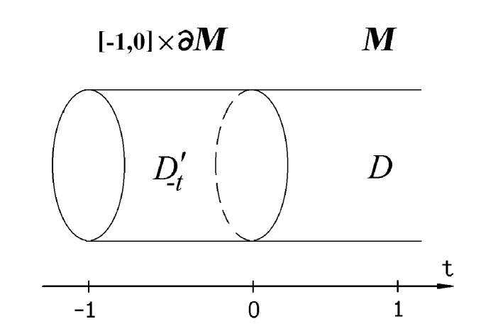
Figure 1: The operator $D$ on the manifold $M^{\prime}=(\left[-1,0\right]\times\partial M)\cup M$

$$M^{\prime}=\left[-1,0\right]\times X\cup M.$$

The operator $D$ can be extended to this manifold: on the cylinder $\left[-1,0\right]\times X$, it is defined by the homotopy $D_{-t}^{\prime}$. The required lifting of the homotopy $\left(D_{\tau}^{\prime},B_{\tau}\right)$ to a homotopy of boundary value problems $\left(D_{\tau},B_{\tau}\right)$ on $M$ is defined by the formula

$$D_{\tau}\left(t,x\right)=D\left(t-\psi\left(t\right)\tau,x\right),\qquad\tau\in\left[0,1\right].$$ (18)

Thus, the boundary value problem $\left(D,B\right)$ is now deformed to a boundary value problem $\left(D_{1},B_{1}\right)$ that coincides near the boundary with the model problem ${\cal D}_{\pm}.$ Hence, we have defined the zero-order elliptic operator

$$\left[{\cal D}_{\pm}^{-1}\circ\left(D_{1},B_{1}\right)\right]\in{\rm\mathop{Ell}}^{0}\left(M\right).$$

It can be verified that this construction defines a homomorphism of groups

$$\begin{array}[]{ccc}\varepsilon_{1}:{\rm\mathop{Ell}}^{1}\left(M\right)&\longrightarrow&{\rm\mathop{Ell}}{}^{0}\left(M\right),\\ \left[D,B\right]&\longmapsto&\left[{\cal D}_{\pm}^{-1}\circ\left(D_{1},B_{1}\right)\right].\end{array}$$

Indeed, this construction is uniquely determined; it takes direct sums of boundary value problems to sums of the corresponding elements; the model operators are taken to zero; finally, the construction is homotopy invariant. It follows from the definition of stable homotopies for boundary value problems that this mapping is the inverse of the order-increasing mapping (13). This establishes the reduction of classical boundary value problems of order one to operators of order zero. The theorem is thereby proved.

2.3 Order reduction: from an arbitrary order to order one

Definition 2

Elliptic boundary value problems ${\cal D}_{1}$ and ${\cal D}_{2}$ of order $m\geq 2$are said to be stably homotopic if for some model operators  ${\cal D}_{\pm}$ and ${\cal D}_{\pm}^{\prime}$ there exists a homotopy between the boundary value problems

$${\cal D}_{1}\oplus{\cal D}_{\pm}D_{+}^{m-1}\quad{\mbox{{\em and}}}\qquad{\cal D}_{2}\oplus{\cal D}_{\pm}^{\prime}D_{+}^{m-1}.$$

The group of stable homotopy classes of boundary value problems for operators of order $m$ is denoted by ${\rm\mathop{Ell}}^{m}\left(M\right)$.

Theorem 3

The mapping

$$\left(\times D_{+}\right)^{m-1}:{\rm\mathop{Ell}}^{1}\left(M\right)\longrightarrow{\rm\mathop{Ell}}^{m}\left(M\right),$$

which increases the order by $m-1$, is an isomorphism of abelian groups.

Proof. Consider a boundary value problem $\left(D,B\right)$ for an operator $D$ of order $m.$ The direct sum

$$\left(D,B\right)\oplus\bigoplus\limits_{1}^{m-1}D_{+}^{m}$$ (19)

defines the same element in the group ${\rm\mathop{Ell}}^{m}\left(M\right)$ as the original problem $\left(D,B\right)$. Let us construct a homotopy of the boundary value problem (19) to the composition of a boundary value problem for an operator of order one and the operator $D_{+}^{m-1}.$ As in the proof of Theorem 2 (see (18)), it suffices to construct the corresponding homotopy of the restriction of $D$ to the boundary together with the boundary conditions.

Let us represent $D$ in the form

$$D=\sum\limits_{k=0}^{m}D_{k}\left(-i\frac{\partial}{\partial t}-i\Lambda_{X}\right)^{k}\left(-i\frac{\partial}{\partial t}+i\Lambda_{X}\right)^{m-k}\equiv\sum\limits_{k=0}^{m}D_{k}D_{-}^{k}D_{+}^{m-k},$$

where $\Lambda_{X}$ is again a first-order operator with principal symbol $\left|\xi^{\prime}\right|$ and the $D_{k}$ are zero-order pseudodifferential operators on $X$. By virtue of condition (7), we can assume that the sum

$$\sum\limits_{k=0}^{m}D_{k}$$

is equal to the identity operator. Consider the operator homotopy

$$D_{\tau}^{\prime}=\left(\begin{array}[]{cccc}D+\tau^{m}D_{0}D_{+}^{m}-\tau^{m}D&\tau^{m-1}D_{1}D_{+}^{m}&\ldots&\tau D_{m-1}D_{+}^{m}+\tau D_{m}D_{-}D_{+}^{m-1}\\ -\tau D_{-}D_{+}^{m-1}&D_{+}^{m}&\ldots&0\\ 0&-\tau D_{-}D_{+}^{m-1}&\ldots&0\\ \ldots&\ldots&\ddots&\ldots\\ 0&0&\ldots&D_{+}^{m}\end{array}\right).$$

At the initial point $\tau=0$, we have

$$D_{\tau=0}^{\prime}=D\oplus\bigoplus\limits_{1}^{m-1}D_{+}^{m}.$$

On the other hand, at $\tau=1$ we obtain the factorization required in the theorem:

$$D_{\tau=1}^{\prime}=\left(\begin{array}[]{cccc}D_{0}D_{+}&D_{1}D_{+}&\ldots&D_{m-1}D_{+}+D_{m}D_{-}\\ -D_{-}&D_{+}&0&0\\ 0&-D_{-}&D_{+}&\ldots\\ 0&0&\ldots&D_{+}\end{array}\right)\circ mD_{+}^{m-1}.$$

The coefficient of $\left(-i\frac{\partial}{\partial t}\right)^{m}$ in the operator $D_{\tau}^{\prime}$ is equal to the composition

$$D_{\tau m}^{\prime}=\left(\begin{array}[]{cccc}1&\tau^{m-1}\left(D_{1}+\ldots+D_{m}\right)&\ldots&\tau\left(D_{m-1}+D_{m}\right)\\ 0&1&\ldots&0\\ 0&0&1&\ldots\\ 0&0&\ldots&1\end{array}\right)\circ\left(\begin{array}[]{cccc}1&0&\ldots&0\\ -\tau&1&\ldots&0\\ 0&-\tau&1&\ldots\\ 0&0&\ldots&1\end{array}\right).$$

Thus, for the operators

$$D_{\tau}=\left(D_{\tau m}^{\prime}\right)^{-1}D_{\tau}^{\prime}$$

the corresponding coefficient is equal to unity. Let us show that the operator $D_{\tau}$ is elliptic for $\tau\in\left[0,1\right]$. To this end, we compute the subspace $L_{+}\left(D_{\tau}\right)$.

Consider a bounded solution

$$U=\left(U_{0}\left(t\right),U_{1}\left(t\right),\ldots,U_{m-1}\left(t\right)\right),\qquad t\rightarrow+\infty,$$

of the equation

$$\sigma\left(D_{\tau}\right)\left(x,\xi^{\prime},-i\frac{d}{dt}\right)U=0,\qquad{\mbox{ for }}\left|\xi^{\prime}\right|=1.{\mbox{ }}$$ (20)

Equation (20) can be replaced by an equivalent equation with the symbol of the operator $D_{\tau}^{\prime}$. The bounded function $U$ is a solution of an ordinary differential equation with constant coefficients; hence, its derivatives are also bounded. The componentwise representation of (20) gives the system

$$\left\{\begin{array}[]{l}\left(1-\tau^{m}\right)\sigma\left(D\right)\left(-i\frac{d}{dt}\right)U_{0}+\left(-i\frac{d}{dt}+i\right)^{m}\left(d_{0}\tau^{m}U_{0}+\ldots+d_{m-1}\tau U_{m-1}\right)+\\ +\tau\left(-i\frac{d}{dt}+i\right)^{m-1}\left(-i\frac{d}{dt}-i\right)d_{m}U_{m-1}=0,\\ \left(-i\frac{d}{dt}+i\right)^{m}U_{j}=\tau\left(-i\frac{d}{dt}+i\right)^{m-1}\left(-i\frac{d}{dt}-i\right)U_{j-1},\qquad{\mbox{ }}0<j<m\end{array}\right.$$ (21)

(the $d_{j}$ are the principal symbols of the operators $D_{j}$). The equation

$$\left(-i\frac{d}{dt}+i\right)u=0$$

on the half-line $\left\{t\geq 0\right\}$ has only a trivial bounded solution. Hence, the operator $-id/dt+i$ can be canceled in (21) in all equations except for the first. Consequently,

$$\left(-i\frac{d}{dt}+i\right)U_{j}=\tau\left(-i\frac{d}{dt}-i\right)U_{j-1}.$$

Substituting these relations into one another, we obtain

$$\left(-i\frac{d}{dt}+i\right)^{j}U_{j}=\tau^{j}\left(-i\frac{d}{dt}-i\right)^{j}U_{0}.$$

It follows that the first equation in (21) is reduced to the requirement

$$\sigma\left(D\right)\left(-i\frac{d}{dt}\right)U_{0}=0.$$ (22)

We conclude that the operator $D_{\tau}$ is indeed elliptic, since equation (22) has no solutions bounded on the entire line.

Hence, we have obtained the following description of the bundle $L_{+}\left(D_{\tau}\right)$: the projection on the first term in the sum

$$E\oplus\bigoplus\limits_{1}^{m-1}E\stackrel{{\scriptstyle pr}}{{\longrightarrow}}E$$

induces an isomorphism of vector bundles

$$L_{+}\left(D_{\tau}\right)\stackrel{{\scriptstyle pr}}{{\longrightarrow}}L_{+}\left(D\right);$$

the preimage of an element $u\in L_{+}\left(D\right)$ under this mapping is given by the formula

$$U = \left(U_{0},\ldots,U_{m-1}\right),$$ (23)

$$U_{0} = u,$$

$$\left(-i\frac{d}{dt}+i\right)^{j}U_{j} = \tau^{j}\left(-i\frac{d}{dt}-i\right)^{j}U_{0}.$$

Let us decompose the operator of boundary conditions in the same way as $D$:

$$Bj_{X}^{m-1}=\left.\sum\limits_{k=0}^{m-1}B_{k}\left(-i\frac{\partial}{\partial t}-i\Lambda_{X}\right)^{k}\left(-i\frac{\partial}{\partial t}+i\Lambda_{X}\right)^{m-1-k}\right|_{t=0}.$$

This implies that the boundary condition

$$Bj_{X}^{m-1}\circ pr:C^{\infty}\left(M,E\oplus\bigoplus\limits_{1}^{m-1}E\right)\rightarrow C^{\infty}\left(X,G\right)$$

has a factorization: on the subspace $L_{+}\left(D_{\tau=1}\right)$, by virtue of (23), we have

$$\sigma\left(B\right)j_{X}^{m-1}\circ pr=\sigma\left(B^{\prime}\right)j_{X}\circ\left(-i\frac{d}{dt}+i\right)^{m-1},\qquad{\mbox{where }}\left(\sigma\left(B^{\prime}\right)j_{X}\right)U=\sum\limits_{k=0}^{m-1}b_{k}U_{k}\left(0\right).$$

That is why the homotopy of boundary value problems

$$\left(D_{\tau},B\circ pr\right),\qquad\tau\in\left[0,1\right],$$ (24)

connects the initial problem (19) with the composition of a boundary value problem for a first-order operator and the operator $D_{+}^{m-1}$:

$$\left(D_{\tau=1},B\circ pr\right)=\left(D^{\prime},B^{\prime}\right)\circ mD_{+}^{m-1}.$$ (25)

One can show that the correspondence between the boundary value problems $\left(D,B\right)$ and $\left(D^{\prime},B^{\prime}\right)$ for operators of order one induces a mapping

$$\varepsilon_{m}^{\prime}:{\rm\mathop{Ell}}^{m}\left(M\right)\longrightarrow{\rm\mathop{Ell}}^{1}\left(M\right).$$

Let us check that this mapping is the inverse of the mapping $\times D_{+}^{m-1}.$ Indeed, the homotopy (24) shows that the group ${\rm\mathop{Ell}}^{m}\left(M\right)$ is generated by compositions of operators (25), i.e. by the range of the mapping $\times D_{+}^{m-1}.$ Hence, this mapping is onto. Let us prove that

$$\varepsilon_{m}^{\prime}\circ\left(\times D_{+}^{m-1}\right)=Id.$$

Indeed, for an elliptic boundary value problem $\left(D^{\prime},B^{\prime}\right)\circ D_{+}^{m-1}$ of order $m$, the matrix of the operator $D_{\tau}$ in the homotopy (24) is a product of two triangular matrices with constant diagonal entries (with respect to the parameter $\tau$ of the homotopy). Thus, this homotopy is trivial, i.e., homotopic to a constant homotopy.

Theorem 3 is thereby proved.

2.4 Main theorems

The above results on the homotopy classification of boundary value problems of fixed order are summarized in the following theorems.

Theorem 4

(the Atiyah–Bott obstruction to the existence of elliptic boundary value problems) For an elliptic operator $D$ on a manifold $M$ with boundary $X$, the following conditions are equivalent.

1. The operator $D$ stably, i.e. up to the direct sum with an operator of the form $D_{+}^{m-1}{\cal D}_{\pm}$ (cf. Definitions 1, 2), admits an elliptic boundary value problem;

2. The following inclusion holds:

   $$\left[L_{+}\left(D\right)\right]\in\pi^{*}K\left(X\right),\quad\pi:S^{*}X\rightarrow X;$$

3. The restriction $\!\left.\sigma\left(D\right)\right|_{X}$ of the principal symbol of the operator to the boundary $\!X\!$ is stably homotopic to the symbol of a multiplication operator;

4. $j^{*}\left[\sigma\left(D\right)\right]=0$ for $j^{*}:K\left(T^{*}M\right)\!\rightarrow\!K\left(T^{*}X\times{\bf R}\right)=K^{1}\left(T^{*}X\right),$ where $j:\left.T^{*}M\right|_{X}\rightarrow T^{*}M$ is the inclusion.

Proof. The equivalence of conditions 1) and 2) follows from the definition of ellipticity for boundary value problems. The equivalence of 3) and 4) is a consequence of the definition of the group $K\left(T^{*}X\times{\bf R}\right)$ in terms of the difference construction.

Let us check the equivalence of conditions 2) and 4). By virtue of homotopies constructed in Theorems 2 and 3, it can be assumed that the operator $D$ in a neighborhood of the boundary has the form

$$D=\frac{\partial}{\partial t}+\Lambda_{X}\left(2P-1\right).$$ (26)

For the operator (26), the following formula is valid:

$$j^{*}\left[\sigma\left(D\right)\right]=\delta\left[L_{+}\left(D\right)\right],\quad\delta:K\left(S^{*}X\right)\rightarrow K^{1}\left(T^{*}X\right).$$

The kernel of the homomorphism $\delta$ coincides with the subgroup $\pi^{*}K\left(X\right)\subset K\left(S^{*}X\right)$ [14]. This implies the equivalence of 2) and 4). The theorem is thereby proved.

Theorem 5

(the homotopy classification of elliptic boundary value problems) For $m\geq 1$, there is an isomorphism of groups

$$\varepsilon_{m}:{\rm\mathop{Ell}}^{m}\left(M\right)\longrightarrow{\rm\mathop{Ell}}^{0}\left(M\right)$$

that is the inverse of the order-increasing mapping

$$\times D_{+}^{m}:{\rm\mathop{Ell}}^{0}\left(M\right)\longrightarrow{\rm\mathop{Ell}}^{m}\left(M\right).$$

Moreover, the following symbol isomorphism holds:

$$\chi:{\rm\mathop{Ell}}^{0}\left(M\right)\longrightarrow K\left(T^{*}\left(M\backslash\partial M\right)\right).$$

Corollary 1

For elliptic boundary value problems ${\cal D}$, one has the equation

$${\rm\mathop{ind}}{\cal D}={\rm\mathop{ind}}\varepsilon_{m}\left[{\cal D}\right],\qquad m\geq 1,$$

and the index formula

$${\rm\mathop{ind}}D=p_{!}\left[\sigma\left(D\right)\right],\quad$$ (27)

where

$$p:M\to pt$$

and

$$\left[\sigma\left(D\right)\right]\in K\left(T^{*}\left(M\backslash\partial M\right)\right)$$

for an operator $D$ of order zero representing $\varepsilon_{m}[{\cal D}]$.

Proof. The mapping $\varepsilon_{m}$ preserves the index by definition. Equation (27) is a special case of the “excision” property of the index (see [11]).

Corollary 2

(cobordism invariance of the index) Let $M$ be a compact manifold with boundary $X$. We denote the natural inclusion mapping by

$$j:X\longrightarrow M.$$

Consider the induced mapping

$$j^{*}:K^{1}\left(T^{*}M\right)\rightarrow K\left(T^{*}X\right)$$

in $K$-theory. If an elliptic operator $D$ over $X$ satisfies the inclusion

$$\left[\sigma\left(D\right)\right]\in{\rm Im}\,j^{*},$$

then

$${\rm\mathop{ind}}D=0.$$

Proof. The desired statement follows from the commutative diagram

$$\begin{array}[]{ccccc}K^{1}\left(T^{*}M\right)&\rightarrow&K\left(T^{*}X\right)&\rightarrow&K\left(T^{*}\left(M\backslash\partial M\right)\right)\\ &&\chi\uparrow&&\uparrow\\ &&{\rm\mathop{Ell}}\left(X\right)&\stackrel{{\scriptstyle\alpha}}{{\rightarrow}}&{\rm\mathop{Ell}}^{1}\left(M\right).\end{array}$$

Here the upper row is induced by the exact sequence of the triple

$$S^{*}M\subset\partial B^{*}M\subset B^{*}M,$$

$\chi$ stands for the difference construction on the (closed) manifold $X$, and the mapping $\alpha$ takes each elliptic operator

$$B:C^{\infty}\left(X,{\bf C}^{N}\right)\rightarrow C^{\infty}\left(X,G\right)$$

to the boundary value problem

$$\left\{\begin{array}[]{ll}D_{-}u=f,&\quad u,f\in C^{\infty}\left(M,{\bf C}^{N}\right),\vspace{0.2cm}\\ Bj_{X}u=g,&\ \quad g\in C^{\infty}\left(X,G\right).\end{array}\right.$$

3 Boundary value problems for general elliptic equations

3.1 Spectral boundary value problems

For an arbitrary elliptic operator $D$, which in general does not satisfy the Atiyah–Bott condition (see Theorem 4 in the previous section), boundary value problems of the following form were introduced in [3]:

$$\left\{\begin{array}[]{ll}Du=f,&u\in H^{s}\left(M,E\right),\quad f\in H^{s-m}\left(M,F\right),\vspace{0.2cm}\\ Bj_{X}^{m-1}u=g,&g\in{\rm Im}\,P\subset H^{\sigma}\left(X,G\right),\end{array}\right.$$ (28)

where the subspace ${\rm Im}\,P$ is the range of a pseudodifferential projection $P$ of order zero in a Sobolev space on the boundary. It was also shown in [3] that the boundary value problem (28) is Fredholm if and only if it is elliptic, i.e., its boundary symbol

$$\sigma\left(B\right):L_{+}\left(D\right)\rightarrow{\rm Im}\,\sigma\left(P\right)$$

is a bundle isomorphism. This class of boundary value problems does not carry obstructions of the Atiyah–Bott type, since for an arbitrary elliptic operator $D$ there exists a so-called spectral boundary value problem, which has the Fredholm property [7].

Example The spectral boundary value problem for an operator of order one.

Let $D$ be a first-order elliptic operator. In a neighborhood of the boundary, it has the form

$$D=\gamma\left(t\right)\left(\frac{\partial}{\partial t}+A\right),$$

where $\gamma(t)$ is a bundle isomorphism. The ellipticity of $D$ implies that the principal symbol $\sigma\left(A\right)\left(x,\xi^{\prime}\right)$ has no pure imaginary eigenvalues for $\left|\xi^{\prime}\right|=1.$ Thus, the family

$$ip+A$$

is elliptic in the sense of Agranovich–Vishik in some sector containing the real line $\left\{p\in{\bf R}\right\}$. It was proved in [7] that the spectral projection $P_{+}$ of the operator $A$ on the subspace corresponding to spectral points with nonnegative real parts along the corresponding negative subspace is a pseudodifferential projection. Its principal symbol $\sigma\left(P_{+}\right)$ is equal to the nonnegative spectral projection for the principal symbol of $A$:

$$\sigma\left(P_{+}\left(A\right)\right)=P_{+}\sigma\left(A\right).$$ (29)

Definition 3

The spectral boundary value problem (cf. [6]) for the operator $D$ is the system of equations of the form

$$\left\{\begin{array}[]{ll}Du=f,&u\in H^{s}\left(M,E\right),f\in H^{s-1}\left(M,F\right),\vspace{0.2cm}\\ P_{+}\left.u\right|_{X}=g,&g\in{\rm Im}\,P_{+}.\end{array}\right.$$ (30)

This boundary value problem has the Fredholm property, since Eq. (29) implies that its boundary symbol is the identity mapping

$${\rm Im}\,P_{+}\sigma\left(A\right)\stackrel{{\scriptstyle Id}}{{\longrightarrow}}{\rm Im}\,\sigma\left(P_{+}\right),\qquad L_{\pm}\left(D\right)={\rm Im}\,P_{\pm}\sigma\left(A\right).$$

3.2 The reduction theorem

The group of stably homotopic boundary value problems (28) for operators of order $m\geq 1$ will be denoted by ${\rm\mathop{Ell}}^{m}\left(M,\partial M\right)$, and the group of stably homotopic spectral boundary value problems for first-order operators will be denoted by ${\rm\mathop{Spec}}\left(M,\partial M\right).$ Here homotopies are families of boundary value problems (28) such that $D$, $B$, and $P$ continuously depend on the parameter and the trivial problems used in stabilization are the same as in the case of classical boundary value problems, i.e., have the form ${\cal D}_{\pm}D_{+}^{m-1}$.

The violation of the Atiyah–Bott condition makes it impossible to reduce boundary value problems to zero-order operators. Nevertheless, the homotopies of the classical theory, described in Section 2, can be generalized to the present situation. They result in the following theorems.

Theorem 6

A boundary value problem for an operator of order $m\geq 2$ can be reduced to a first-order boundary value problem. In other words, there is an isomorphism of groups

$${\rm\mathop{Ell}}^{m}\left(M,\partial M\right)\longrightarrow{\rm\mathop{Ell}}^{1}\left(M,\partial M\right)$$

that is the inverse of the order-increasing mapping

$$\times D_{+}^{m-1}:{\rm\mathop{Ell}}^{1}\left(M,\partial M\right)\longrightarrow{\rm\mathop{Ell}}^{m}\left(M,\partial M\right).$$

Theorem 7

A boundary value problem for a first-order operator can be reduced to a spectral boundary value problem. In other words, there is an isomorphism of groups

$${\rm\mathop{Ell}}^{1}\left(M,\partial M\right)\longrightarrow{\rm\mathop{Spec}}\left(M,\partial M\right).$$

The proof of Theorem 6 coincides with that of the similar theorem (Theorem 3) for classical boundary value problems, since the formulas given there do not take into account the classical type of boundary value problems.

Proof of Theorem 7. Consider the boundary value problem (28). The first homotopy (14) in the proof of Theorem 2 can be generalized without changes. Let us substitute the pseudodifferential projection $P$ that defines the boundary values into the rotation homotopy (15) instead of $P_{G}$. In the end of the homotopy (16), (17), we obtain the spectral boundary value problem

$$\begin{array}[]{c}D_{\pi/2}^{\prime}=\gamma\left(\frac{\partial}{\partial t}+\Lambda_{X}\left(2P-1\right)\right),\\ \\ B_{\pi/2}=P:C^{\infty}\left(X,\left.E\right|_{X}\oplus{\bf C}^{N}\right)\longrightarrow{\rm Im}\,P\subset C^{\infty}\left(X,\left.E\right|_{X}\oplus{\bf C}^{N}\right).\end{array}$$

Thus, an arbitrary first-order boundary value problem can be reduced to a spectral boundary value problem whose spectral subspace coincides with the subspace of boundary values of the initial problem. This proves the theorem.

In the general case, the reduction of a boundary value problem to an operator of order zero is impossible by the Atiyah–Bott condition. In the next section, we discuss a class of boundary value problems for which the Atiyah–Bott condition is satisfied rationally. The reduction to classical boundary value problems is carried out (also rationally) in this case.

4 Boundary value problems in even and odd subspaces

4.1 Parity conditions

On the cotangent bundle of the manifold $M$, we consider the antipodal involution

$$\alpha:T^{*}M\longrightarrow T^{*}M,\qquad\\ \alpha\left(x,\xi\right)=\left(x,-\xi\right).$$

Definition 4

A pseudodifferential projection $P$ of order zero is said to be even (odd) if its homogeneous principal symbol on the sphere bundle $S^{*}M$ is invariant (antiinvariant) with respect to the involution $\alpha$:

$$\alpha^{*}\sigma\left(P\right)=\sigma\left(P\right)\qquad{\rm or}\qquad\sigma\left(P\right)+\alpha^{*}\sigma\left(P\right)=1.$$

To a spectral boundary value problem $\left(D,P\right)$ with a first-order operator $D$ and an even (odd) projection $P$, one can assign a classical boundary value problem. To this end, let us denote by $\alpha^{*}D$ and $\alpha^{*}D^{-1}$ first-order elliptic operators with principal symbols equal to $\alpha^{*}\sigma\left(D\right)$ and $\alpha^{*}\sigma^{-1}\left(D\right)$, respectively, on the sphere bundle $S^{*}M$. In the even case, the operator $D\oplus\alpha^{*}D$ admits the elliptic classical boundary value problem

$$\left\{\begin{array}[]{c}Du=f_{1},\qquad\alpha^{*}Dv=f_{2},\vspace{0.2cm}\\ P\left.u\right|_{X}+\left(1-P\right)\left.v\right|_{X}=g,\quad g\in C^{\infty}\left(X,\left.E\right|_{X}\right).\end{array}\right.$$ (31)

Likewise, in the odd case we have the boundary value problem

$$\left\{\begin{array}[]{c}Du=f_{1},\qquad\alpha^{*}D^{-1}v=f_{2},\vspace{0.2cm}\\ P\left.u\right|_{X}+\left(1-P\right)\left.v\right|_{X}=g,\quad g\in C^{\infty}\left(X,\left.E\right|_{X}\right).\end{array}\right.$$ (32)

In the passage from the spectral boundary value problem $\left(D,P\right)$ to the classical boundary value problem (31) or (32), the dimension of the manifold $M$ must be taken into account. The following proposition shows that if the parity of the boundary value problem is opposite to the parity of ${\rm dim}M$, then the boundary value problems (31) and (32) define $2$-torsion elements in the group ${\rm\mathop{Ell}}^{1}\left(M\right)\simeq K(T^{*}(M\setminus\partial M))$.

Proposition 2

1. The mapping $\alpha$ induces an involution in $K$-theory. Modulo $2$-torsion, this involution is equal to $\left(-1\right)^{\dim M}:$

   $$\alpha^{*}:K^{*}\left(T^{*}M\right)\otimes{\bf Z}\left[\frac{1}{2}\right]\longrightarrow K^{*}\left(T^{*}M\right)\otimes{\bf Z}\left[\frac{1}{2}\right],\quad\alpha^{*}=\left(-1\right)^{\dim M}.$$

   The involution $\alpha^{*}$ has this property also on the group $K^{*}\left(T^{*}\left(M\backslash\partial M\right)\right).$

2. For an even-dimensional manifold $M$, the projection $S^{*}M\rightarrow P^{*}M$induces an isomorphism (modulo $2$-torsion)

   $$K^{*}\left(P^{*}M\right)\otimes{\bf Z}\left[\frac{1}{2}\right]\rightarrow K^{*}\left(S^{*}M\right)\otimes{\bf Z}\left[\frac{1}{2}\right]$$

   (here $P^{*}M=S^{*}M/\alpha$ is the corresponding projective cotangent sphere bundle).

3. On an odd-dimensional manifold, the projection $P^{*}M\rightarrow M$ induces an isomorphism (modulo $2$-torsion)

   $$K^{*}\left(M\right)\otimes{\bf Z}\left[\frac{1}{2}\right]\rightarrow K^{*}\left(P^{*}M\right)\otimes{\bf Z}\left[\frac{1}{2}\right].$$

Proof. Let us apply the Mayer–Vietoris principle [15].

1) Let us check properties 1–3 for the restriction of the mappings to the fiber over a point $x$ of the base $M$ of the corresponding bundles:

$$K^{*}\left(T_{x}^{*}M\right) \longrightarrow K^{*}\left(T_{x}^{*}M\right),$$

$$\,K^{*}\left(P_{x}^{*}M\right) \rightarrow K^{*}\left(S_{x}^{*}M\right),$$

$$K^{*}\left(\left\{x\right\}\right) \rightarrow K^{*}\left(P_{x}^{*}M\right).$$

In the first case, we have

$$T_{x}^{*}M={\bf R}^{\dim M},\qquad K^{*}\left({\bf R}^{\dim M}\right)={\bf Z.}$$

The involution $\alpha$ preserves (or reverses) the orientation of the space ${\bf R}^{\dim M}$ depending on the parity of dimension of $M$. Hence, we obtain the desired identity $\alpha^{*}=\left(-1\right)^{\dim M}.$

In the second case, for an even-dimensional manifold $M$ we consider the projection $\pi:S^{2n+1}\rightarrow{\bf RP}^{2n+1}$. The $K$-groups of spheres and projective spaces are well-known (e.g., see [16]):

$$K^{0}\left({\bf RP}^{2n+1}\right) = {\bf Z\oplus Z}_{2^{n}},\quad K^{0}\left(S^{2n+1}\right)={\bf Z,}$$

$$K^{1}\left({\bf RP}^{2n+1}\right) = {\bf Z,\qquad}\quad K^{1}\left(S^{2n+1}\right)={\bf Z.}$$

The first term in the groups $K^{0}$ is given by the dimension of vector bundles, while the projection $\pi$ induces the multiplication by 2 mapping on the groups $K^{1}$:

$$\begin{array}[]{ccc}\pi^{*}:K^{1}\left({\bf RP}^{2n+1}\right)={\bf Z}&{\bf\longrightarrow}&K^{1}\left(S^{2n+1}\right)={\bf Z},\\ n&\longmapsto&2n.\end{array}$$

In the third case, on an odd-dimensional $M$ we consider the projection ${\bf RP}^{2n}\rightarrow pt.$ The relevant $K$-groups are

$$K^{0}\left({\bf RP}^{2n}\right) = {\bf Z\oplus Z}_{2^{n}},\quad K^{0}\left(pt\right)={\bf Z,}$$

$$K^{1}\left({\bf RP}^{2n+1}\right) = 0,\qquad K^{1}\left(pt\right)=0{\bf.}$$

Both components ${\bf Z}$ correspond to the dimension of vector bundles. Thus, property $3$ is also satisfied over a point.

2) By the Mayer–Vietoris principle, we have to verify the following assertion: if properties 1–3 are satisfied over open subsets $U,V\subset M$ and their intersection $U\cap V,$ then these properties hold over the union $U\cup V$.

In the first case, let us write out a part of the Mayer–Vietoris exact sequence

$$\begin{array}[]{ccccc}K^{*+1}\left(T^{*}\left(U\bigcap V\right)\right)&\rightarrow&K^{*}\left(T^{*}\left(U\bigcup V\right)\right)&\rightarrow&K^{*}\left(T^{*}U\right)\oplus K^{*}\left(T^{*}V\right)\\ \downarrow\alpha^{*}&&\downarrow\alpha^{*}&&\quad\quad\quad\downarrow\!\!\alpha^{*}\!\!\oplus\!\alpha^{*}\\ K^{*+1}\left(T^{*}\left(U\bigcap V\right)\right)&\rightarrow&K^{*}\left(T^{*}\left(U\bigcup V\right)\right)&\rightarrow&K^{*}\left(T^{*}U\right)\oplus K^{*}\left(T^{*}V\right).\end{array}$$

A diagram chase shows that the mapping $\alpha^{*}$ in the middle satisfies property 1.

The second and the third cases can be treated in a similar way. For example, on an even-dimensional $M$, the projection $\pi:S^{*}M\rightarrow P^{*}M$ acts on the Mayer–Vietoris sequences

$$\begin{array}[]{cccc}\cdots\rightarrow\!&K^{*}\left(P^{*}\left(U\bigcup V\right)\right)\!\rightarrow\!&K^{*}\left(P^{*}\left(U\sqcup V\right)\right)\rightarrow&K^{*}\left(P^{*}\left(U\bigcap V\right)\right)\rightarrow\cdots\\ &\downarrow\pi^{*}&\quad\downarrow\!\!\pi^{*}\!&\downarrow\pi^{*}\\ \cdots\rightarrow\!&K^{*}\left(S^{*}\left(U\bigcup V\right)\right)\!\rightarrow\!&K^{*}\left(S^{*}\left(U\sqcup V\right)\right)\rightarrow&K^{*}\left(S^{*}\left(U\bigcap V\right)\right)\rightarrow\cdots\end{array}$$

By the five lemma, the mapping $\pi^{*}$ on the left is an isomorphism modulo 2-torsion.

The statement concerning the group $K^{*}\left(T^{*}\left(M\backslash\partial M\right)\right)$ follows from the exact sequence of the pair $\left.T^{*}M\right|_{X}\subset T^{*}M$ on which $\alpha^{*}$ acts:

$$\begin{array}[]{ccccccc}\rightarrow\!\!&K^{*+1}\left(\left.T^{*}M\right|_{X}\right)\otimes{\bf Z}\left[\frac{1}{2}\right]&\!\!\rightarrow\!\!&K^{*}\left(T^{*}\left(M\backslash\partial M\right)\right)\otimes{\bf Z}\left[\frac{1}{2}\right]&\rightarrow&K^{*}\left(T^{*}M\right)\otimes{\bf Z}\left[\frac{1}{2}\right]&\!\!\rightarrow\\ &\qquad\downarrow\left(-1\right)^{\dim M}&&\downarrow\alpha&&\qquad\downarrow\left(-1\right)^{\dim M}&\\ \rightarrow\!\!&K^{*+1}\left(\left.T^{*}M\right|_{X}\right)\otimes{\bf Z}\left[\frac{1}{2}\right]&\!\!\rightarrow\!\!&K^{*}\left(T^{*}\left(M\backslash\partial M\right)\right)\otimes{\bf Z}\left[\frac{1}{2}\right]&\rightarrow&K^{*}\left(T^{*}M\right)\otimes{\bf Z}\left[\frac{1}{2}\right]&\!\!\rightarrow\end{array}$$

This completes the proof of Proposition 2.

Thus, in what follows we consider boundary value problems with even projections $P$ on even-dimensional manifolds and odd projections on odd-dimensional manifolds.

4.2 The classification of boundary value problems with even projections

The boundary value problem (30) in subspaces cannot be classified in terms of the classical boundary value problem (31) or (32) even under the above parity restrictions. The point is that a classical boundary value problem is defined, up to a homotopy, by its principal symbol, while the boundary value problem (30) is not determined by the principal symbol. Indeed, by adding finite-dimensional spaces to ${\rm Im}\,P$, we obtain boundary value problems with the same principal symbol but with different index, which shows that they are not homotopic to the original problem.

It is shown in [8, 9] that the subspaces defined by even (odd) pseudodifferential projections have the homotopy invariant described in the following theorem. Let us denote the semigroups of subspaces defined by even (odd) pseudodifferential projections by $\widehat{{\rm\mathop{Even}}}\left(X\right)$ and $\widehat{{\rm\mathop{Odd}}}\left(X\right)$, respectively.

Theorem 8

[8, 9] There is a unique homotopy invariant functional $d$

$$d:\widehat{{\rm\mathop{Even}}}\left(X^{odd}\right)\rightarrow{\bf Z}\left[\frac{1}{2}\right],\quad{\mbox{or \quad}}d:\widehat{{\rm\mathop{Odd}}}\left(X^{ev}\right)\rightarrow{\bf Z}\left[\frac{1}{2}\right],$$

with the following properties:

1. (invariance)

   $$d\left({\rm Im}\,UPU^{-1}\right)=d\left({\rm Im}\,P\right)$$

   for invertible pseudodifferential operators $U$with even principal symbol: $\alpha^{*}\sigma\left(U\right)=\sigma\left(U\right)$;

2. (relative index)

   $$d\left({\rm Im}\,P_{1}\right)-d\left({\rm Im}\,P_{2}\right)={\rm\mathop{ind}}\left(P_{1},P_{2}\right),$$

   where ${\rm ind}(P_{1},P_{2})={\rm ind}(P_{2}:{\rm Im}\,P_{1}\to{\rm Im}\,P_{2})$ is the relative index of projections with equal principal symbols [17];

3. (complement)

   $$d\left({\rm Im}\,P\right)+d\left({\rm Im}\,\left(1-P\right)\right)=0.$$

The group of stably homotopic spectral boundary value problems with even projections $P$ is denoted by ${\rm\mathop{Ell}}^{ev}\left(M,\partial M\right).$ It turns out that the classical boundary value problem (31) and the invariant $d$ of the subspace of right-hand sides already classify spectral boundary value problems modulo $2$-torsion.

Theorem 9

On an even-dimensional manifold $M$, the mapping

$$\begin{array}[]{ccc}\chi:{\rm\mathop{Ell}}^{ev}\left(M,\partial M\right)\otimes{\bf Z}\left[\frac{1}{2}\right]&\rightarrow&{\rm\mathop{Ell}}^{1}\left(M\right)\otimes{\bf Z}\left[\frac{1}{2}\right]\oplus{\bf Z}\left[\frac{1}{2}\right],\\ &&\\ \left(D,P\right)&\longmapsto&\left(\left(D\oplus\alpha^{*}D\right)\otimes\frac{1}{2},d\left({\rm Im}\,P\right)\right)\end{array}$$

is an isomorphism of abelian groups.

Proof. Let us define the inverse mapping

$$\chi^{\prime}:{\rm\mathop{Ell}}^{1}\left(M\right)\otimes{\bf Z}\left[\frac{1}{2}\right]\oplus{\bf Z}\left[\frac{1}{2}\right]\rightarrow{\rm\mathop{Ell}}^{ev}\left(M,\partial M\right)\otimes{\bf Z}\left[\frac{1}{2}\right].$$

On the first term it is induced by the embedding of classical boundary value problems in boundary value problems with even projections, while on the second term it is given by the formula

$$\chi^{\prime}\left(0,\frac{k}{2^{N}}\right)=\frac{1}{2^{N}}\left(D_{+},k\right),$$

where $\left(D_{+},k\right)$ stands for the spectral boundary value problem for the operator $D_{+}$ with a finite-dimensional spectral projection of rank $k.$ Let us verify that $\chi^{\prime}$ is the inverse of $\chi.$

The second component of the composition $\chi\circ\chi^{\prime}$

$${\bf Z}\left[\frac{1}{2}\right]\rightarrow{\bf Z}\left[\frac{1}{2}\right]$$

is the identity mapping by property 2) of the functional $d.$ The first component is equal to

$$\frac{\alpha^{*}+1}{2}:{\rm\mathop{Ell}}^{1}\left(M\right)\otimes{\bf Z}\left[\frac{1}{2}\right]\longrightarrow{\rm\mathop{Ell}}^{1}\left(M\right)\otimes{\bf Z}\left[\frac{1}{2}\right],$$

which, by virtue of the isomorphism

$${\rm\mathop{Ell}}^{1}\left(M\right)\simeq K\left(T^{*}\left(M\backslash\partial M\right)\right)$$

and Proposition 2, item 1, is the identity mapping.

The assertion of the theorem can now be derived from the following lemma.

Lemma 1

The homomorphism $\chi^{\prime}$ is an epimorphism.

Proof. Consider an arbitrary spectral boundary value problem $\left(D,P\right)$ with even projection $P$. Proposition 2, item 3 implies that the sum of $2^{N}$ copies of the subbundle ${\rm Im}\,\sigma\left(P\right)\subset\pi^{*}E$ is homotopic in the class of even subbundles to a bundle $\pi^{*}G,$ $G\subset E^{2^{N}}$, lifted from the base $X$. We denote the corresponding homotopy of projections by $\sigma\left(P_{t}\right)$:

$$\sigma\left(P_{t}\right):\pi^{*}E^{2^{N}}\longrightarrow\pi^{*}E^{2^{N}},\qquad t\in\left[0,1\right],$$

$$\sigma\left(P_{0}\right)=2^{N}\sigma\left(P\right),\quad{\rm Im}\,\sigma\left(P_{1}\right)=\pi^{*}G.$$

Consider a covering homotopy of pseudodifferential projections $P_{t}$ such that $P_{0}=2^{N}P.$ The symbol of $P_{1}$ is equal to the symbol of projection $P_{G}$ on the space $C^{\infty}\left(X,G\right)\subset C^{\infty}\left(X,E\right)$ of sections of bundle $G.$ Hence, the homotopy classification of projections with the same principal symbols [18] shows that $P_{1}$ is homotopic to a projection differing from $P_{G}$ by a finite rank projection. We can assume that the homotopy $P_{t}$ already gives such a projection at $t=1$.

The homotopy of projections $P_{t}$ extends to a homotopy of spectral boundary value problems

$$\left(D_{t},P_{t}\right):D_{0}=2^{N}D$$

by formula (16). The spectral boundary value problem $\left(D_{1},P_{1}\right)$ then lies in the range of the mapping $\chi^{\prime}$ given by

$$\chi^{\prime}\left[\left(D_{1},P_{G}\right),-{\rm\mathop{ind}}\left(P_{G},P_{1}\right)\right]=\left[D_{1},P_{1}\right].$$

This proves the lemma. The theorem is thereby proved.

4.3 The classification of boundary value problems with odd projections

Let us generalize the definition of spectral boundary value problems with odd projections. We consider spectral boundary value problems such that the symbol of the projection $P$ is the sum of a constant symbol with respect to the cotangent variables and an odd projection. Let us also identify spectral boundary value problems of the form

$$\left\{\begin{array}[]{c}D_{1}u=f_{1},\qquad D_{2}v=f_{2},\\ P\left.u\right|_{X}=g_{1},\quad\left(1-P\right)\left.v\right|_{X}=g_{2}\end{array}\right.$$ (33)

with odd projection $P$ with the corresponding classical boundary value problems

$$\left\{\begin{array}[]{c}D_{1}u=f_{1},\qquad D_{2}v=f_{2},\\ P\left.u\right|_{X}+\left(1-P\right)\left.v\right|_{X}=g.\end{array}\right.$$ (34)

The abelian group of stable homotopy classes of such spectral boundary value problems will be denoted by ${\rm\mathop{Ell}}^{odd}\left(M,\partial M\right)$. In the following theorem, the stable homotopy classification modulo 2-torsion is established for spectral boundary value problems with odd projections.

Theorem 10

On an odd-dimensional manifold $M$, the mapping

$$\begin{array}[]{ccc}\chi:{\rm\mathop{Ell}}^{odd}\left(M,\partial M\right)\otimes{\bf Z}\left[\frac{1}{2}\right]&\rightarrow&{\rm\mathop{Ell}}^{1}\left(M\right)\otimes{\bf Z}\left[\frac{1}{2}\right]\oplus{\bf Z}\left[\frac{1}{2}\right],\\ &&\\ \left(D,P\right)&\longmapsto&\left(\left(D\oplus\alpha^{*}D^{-1}\right)\otimes\frac{1}{2},d\left({\rm Im}\,P\right)\right)\end{array}$$

is an isomorphism of abelian groups.

Proof. Let us define the inverse mapping

$$\chi^{\prime}:{\rm\mathop{Ell}}^{1}\left(M\right)\otimes{\bf Z}\left[\frac{1}{2}\right]\oplus{\bf Z}\left[\frac{1}{2}\right]\rightarrow{\rm\mathop{Ell}}^{odd}\left(M,\partial M\right)\otimes{\bf Z}\left[\frac{1}{2}\right].$$

On the first summand it is induced by the embedding of classical boundary value problems in the class of boundary value problems with odd projections, and on the second summand it is given, just as in the previous theorem, by the formula

$$\chi^{\prime}\left(0,\frac{k}{2^{N}}\right)=\frac{1}{2^{N}}\left(D_{+},k\right).$$

The second component of the composition $\chi\circ\chi^{\prime}$

$${\bf Z}\left[\frac{1}{2}\right]\rightarrow{\bf Z}\left[\frac{1}{2}\right]$$

is equal to the identity mapping, while the first component is

$$\frac{1-\alpha^{*}}{2}:{\rm\mathop{Ell}}^{1}\left(M\right)\otimes{\bf Z}\left[\frac{1}{2}\right]\longrightarrow{\rm\mathop{Ell}}^{1}\left(M\right)\otimes{\bf Z}\left[\frac{1}{2}\right],$$

and, by virtue of the isomorphism

$${\rm\mathop{Ell}}^{1}\left(M\right)\simeq K\left(T^{*}\left(M\backslash\partial M\right)\right)$$

and Proposition 2, item 1, it is equal to the identity mapping.

The following lemma completes the proof of the theorem.

Lemma 2

The homomorphism $\chi^{\prime}$ is an epimorphism.

Proof. Consider the spectral boundary value problem $\left(D,P\right)$ with an odd projection $P.$ Just as in the proof of Lemma 1, we only need to construct a homotopy of the principal symbol of $P$ to a projection independent of the cotangent variables. By virtue of the identification (33), (34), it suffices to construct a homotopy of the principal symbol of the projection to a direct sum $p\oplus\left(1-p\right)$, where $p$ is an odd projection.

It was proved in [9] that for some $N$ there exists an even isomorphism

$$u:2^{N}\pi^{*}\left.E\right|_{X}\rightarrow 2^{N}\pi^{*}\left.E\right|_{X},\qquad\pi:S^{*}X\rightarrow X,$$

that takes the projection $2^{N}\sigma\left(P\right)$ to the complementary projection $2^{N}\left(1-\sigma\left(P\right)\right)$. Moreover, this isomorphism defines the zero element in the group $K^{1}\left(S^{*}X\right)$. It follows from Proposition 2, item 2 that for sufficiently large $N$ the isomorphism $u$ is homotopic to the identity in the class of even isomorphisms. Let us denote a homotopy of this type by $u_{t}$, $t\in\left[0,1\right]$, $u_{0}=1.$ The desired homotopy of projections is given by the formula

$$\sigma\left(P_{t}\right)=2^{N}\sigma\left(P\right)\oplus u_{t}2^{N}\sigma\left(P\right)u_{t}^{-1},$$

$$\sigma\left(P_{0}\right)=2^{N+1}\sigma\left(P\right),\qquad\sigma\left(P_{1}\right)=2^{N}\left[\sigma\left(P\right)\oplus\left(1-\sigma\left(P\right)\right)\right].$$

The lemma and the theorem are thereby proved.

Corollary 3

[8, 9] Spectral boundary value problems ${\rm\mathop{Ell}}^{ev/odd}\left(M,\partial M\right)$ with parity conditions have the following homotopy classification modulo 2-torsion:

$${\rm\mathop{Ell}}^{ev/odd}\left(M,\partial M\right)\otimes{\bf Z}\left[\frac{1}{2}\right]\simeq K\left(T^{*}(M\setminus\partial M)\right)\otimes{\bf Z}\left[\frac{1}{2}\right]\oplus{\bf Z}\left[\frac{1}{2}\right].$$

The index formula

$${\rm\mathop{ind}}\left(D,P\right)=\frac{1}{2}{\rm\mathop{ind}}\left(D\oplus\alpha^{*}D^{\pm 1}\right)-d\left({\rm Im}\,P\right)$$ (35)

is valid.

Indeed, let us consider both sides of the index formula as homomorphisms of the group ${\rm\mathop{Ell}}^{ev/odd}\left(M,\partial M\right)$ into ${\bf Z}\left[\frac{1}{2}\right]$. By Theorems 9 and 10, the groups ${\rm\mathop{Ell}}^{ev/odd}\left(M,\partial M\right)$ are rationally generated by classical boundary value problems and boundary value problems with finite-dimensional spectral subspaces. On both types of generators, the two parts of the index formula (35) coincide. This proves the index formula.

Moscow, Potsdam

References

- [1] L. Hörmander. The Analysis of Linear Partial Differential Operators. III. Springer-Verlag, Berlin Heidelberg New York Tokyo, 1985.
- [2] M. F. Atiyah and R. Bott. The index problem for manifolds with boundary. In Bombay Colloquium on Differential Analysis, 1964, pages 175–186, Oxford. Oxford University Press.
- [3] B.-W. Schulze, B. Sternin, and V. Shatalov. On general boundary value problems for elliptic equations. Math. Sb., 189, No. 10, 1998, 1573–1586.
- [4] B. Booß-Bavnbek and K. Wojciechowski. Elliptic Boundary Problems for Dirac Operators. Birkhäuser, Boston–Basel–Berlin, 1993.
- [5] L. Boutet de Monvel. Boundary problems for pseudodifferential operators. Acta Math., 126, 1971, 11–51.
- [6] M. Atiyah, V. Patodi, and I. Singer. Spectral asymmetry and Riemannian geometry I. Math. Proc. Cambridge Philos. Soc., 77, 1975, 43–69.
- [7] V. Nazaikinskii, B.-W. Schulze, B. Sternin, and V. Shatalov. Spectral boundary value problems and elliptic equations on singular manifolds. Differents. Uravnenija, 34, No. 5, 1998, 695–708. [Russian].
- [8] A. Yu. Savin and B. Yu. Sternin. Elliptic Operators in Even Subspaces. Univ. Potsdam, Institut für Mathematik, Potsdam, Juni 1999. Preprint N 99/10, Russian Acad. Sci. Sb. Math., 190, No. 8, 1999, 125 – 160, [Russian]. math.DG/9907027.
- [9] A. Yu. Savin and B. Yu. Sternin. Elliptic Operators in Odd Subspaces. Univ. Potsdam, Institut für Mathematik, Potsdam, Juni 1999. Preprint N 99/11, math.DG/9907039.
- [10] P. B. Gilkey. The eta invariant of even order operators. Lecture Notes in Mathematics, 1410, 1989, 202–211.
- [11] M. F. Atiyah and I. M. Singer. The index of elliptic operators I. Ann. of Math., 87, 1968, 484–530.
- [12] S. Rempel and B.-W. Schulze. Index Theory of Elliptic Boundary Problems. Akademie-Verlag, Berlin, 1982.
- [13] M. Agranovich and M. Vishik. Elliptic problems with parameter and parabolic problems of general type. Uspekhi Mat. Nauk, 19, No. 3, 1964, 53–161. English transl.: Russ. Math. Surv. 19 (1964), N 3, p. 53–157.
- [14] M. Atiyah, V. Patodi, and I. Singer. Spectral asymmetry and Riemannian geometry III. Math. Proc. Cambridge Philos. Soc., 79, 1976, 71–99.
- [15] R. Bott and L. Tu. Differential Forms in Algebraic Topology, volume 82 of Graduate Texts in Mathematics. Springer-Verlag, Berlin-Heidelberg-New York, 1982.
- [16] P. B. Gilkey. The Geometry of Spherical Space Form Groups, volume 7 of Series in Pure Mathematics. World Scientific, Singapore, 1989.
- [17] P. Baum, R. Douglas, and P. Fillmore Extensions of -algebras and -homology. Ann. Math. II, 105, 1977, 265–324.
- [18] K. Wojciechowski. A note on the space of pseudodifferential projections with the same principal symbol. J. Operator Theory, 15, No. 2, 1986, 207–216.