IC/99/66

The Universal Perturbative Quantum 3-manifold Invariant, Rozansky-Witten Invariants, and the Generalized Casson Invariant.

Nathan Habegger and George Thompson

Let $Z^{LMO}$ be the 3-manifold invariant of [LMO]. It is shown that $Z^{LMO}(M)=1$, if the first Betti number of $M$, $b_{1}(M)$, is greater than 3. If $b_{1}(M)=3$, then $Z^{LMO}(M)$ is completely determined by the cohomology ring of $M$. A relation of $Z^{LMO}$ with the Rozansky-Witten invariants $Z_{X}^{RW}[M]$ is established at a physical level of rigour. We show that $Z_{X}^{RW}[M]$ satisfies appropriate connected sum properties suggesting that the generalized Casson invariant ought to be computable from the LMO invariant.

1 Introduction

In [W], E. Witten explained the Jones polynomial using physics. In doing so, he introduced mathematicians to the partition function $Z_{G,k}^{CS}(M,L)$ of the topological quantum field theory associated to the Chern Simons action, for a Lie group $G$ and coloured link $L\subset M$. Its physical definition is given by a Feynman path integral over the infinite dimensional space of connections.

In general, one expects that topological field theories defined using the path integral, or perturbative versions of these, can be given a rigorous definition through surgery formulae, just as is the case for other quantum invariants, such as the Reshetikhin-Turaev [RT] invariants, $Z^{RT}_{G,k}$, or the more recent universal invariant $Z^{LMO}$, of T. Le, J. Murakami, and T. Ohtsuki [LMO] and the Århus invariant, $Z^{\AA}$, [BGRT]. Invariants have also been given through integral formulae, as is the case for the Kontsevich integral $Z^{K}$ (see [K] [B]), the Bott-Taubes invariant $Z^{BT}$, [BoTa], [AF], and the invariant $Z^{BC}$ of Bott and Cattaneo [BC], [AC]. (It is conjectured that $Z^{K}=Z^{BT}$.)

Our intent in this paper is to study the invariant $Z^{LMO}(M)$. $Z^{LMO}(M)$ lies in $A(\emptyset)$, the vector space of Feynman diagrams modulo anti-symmetry and $IHX$ relations. This vector space is not well-understood, except in low degrees. (See Vogel, [V], for an attempt to understand the structure of $A(\emptyset)$.)

Quantum invariants (or perturbative versions of these) are a rich source of data for the study of knots, links, and 3-manifolds. Nevertheless, their relationship to classical topology remains obscure, hampering their use in problem-solving. A notable exception is the Alexander polynomial of a knot, which, through its interpretation as the Conway polynomial (together with the solution of the Conway weight system on uni-trivalent graphs [KS]), gives a computation of (the one loop) part of the Kontsevich integral. Another recent advance has been the computation of the Milnor invariants from the Kontsevich integral [HM].

For 3-manifolds, one has the result that the degree one term of the LMO invariant, $Z^{LMO}_{1}$, is the Casson-Walker-Lescop invariant [LMO], [BeHa]. However, beyond this, the topological significance of $Z^{LMO}$ remains a mystery. For example, it is not even known whether or not the degree two term of $Z^{LMO}$ vanishes in the simply connected case (which of course would be implied by a positive solution of the Poincaré conjecture, since $Z^{LMO}(S^{3})=1$).

One possible programme for attempting to tie the quantum invariants to homotopy data is through generalization of the Casson invariant to groups other than $SU(2)$, e.g., $SU(N)$. Recent advances on the mathematical side [BH], for $SU(3)$, as well as on the physical side, by Rozansky and Witten [RW], may make this programme tractable. The purpose of this paper is to give a conjectural relationship between the generalized Casson invariants and $Z^{LMO}$ and some partial evidence for its veracity. We consider this conjecture to be an explicit form of the basic philosophical viewpoint of [RW], who believe their invariants are of finite type.

Indeed, we may summarize the underlying ideas of [RW] as follows. On the one hand a comparison of the Rozansky-Witten invariants to the perturbative Chern-Simons theory indicates that, for $b_{1}(M)=0$, they both arise from one universal theory. The difference between the two rests in the choice of weight system (in [RW] a rigorous mathematical weight system $W_{X}^{RW}$ is given). On the other hand, (and perhaps the deepest part of the theory) equivalence between certain physical theories allows one to identify the Rozansky-Witten invariants for a particular choice of hyper-Kähler manifold $X_{G}$ with a regularized Euler characteristic [BT1] of the moduli space of flat G-connections on the 3-manifold M, $\chi_{G}(M)$. The equivalence comes from the work of Seiberg and Witten on 3-dimensional theories (and is the analogue of their work in four dimensions). The twist of the first theory yields the gauge theoretic model of the Euler characteristic while the twist of the second is the Rozansky-Witten model. The equivalence of the physical theories suggests the equivalence of their twisted topological versions. Thus, from the physics side, one expects that

$$Z^{RW}_{X_{G}}(M)=\chi_{G}(M).$$ (1.1)

One important consequence of (1.1) is its potential use in computing $\chi_{G}(M)$.

On the mathematical side there are, currently, a number of candidates for a universal perturbative quantum invariant. These include the LMO invariant, $Z^{LMO}$, the Århus invariant, $Z^{\AA}$, and the invariant of Bott and Cattaneo, $Z^{BC}$. It has been suggested [BGRT] that although the LMO invariant agrees with the Århus invariant, for rational homology spheres, that nevertheless $Z^{LMO}$ is more directly related to the Rozansky-Witten sigma model theory than to the Chern-Simons gauge theory.

For $b_{1}(M)>0$, (except for $b_{1}(M)=1$ and ${\mathrm{T}or\,H}_{1}(M,{\mathbb{Z}})\neq 0$) the first author and collaborators, [BeHa] [GH], have calculated $Z^{LMO}$ from classical data. Here, we perform analogous computations in the Rozansky-Witten theory and observe, for $b_{1}(M)>0$, that these results agree. Specifically, we show, for $b_{1}(M)>0$, and under the conditions mentioned above, that at the physical level of rigour,

$$W^{RW}_{X}\left(Z_{n}^{LMO}(M)\right)=Z^{RW}_{X}(M),$$ (1.2)

where $X$ denotes a hyper-Kähler manifold of dimension $4n$.

One might naively conjecture that (1.2) holds for all 3-manifolds. However, for $b_{1}(M)=0$, which is the case of most interest, numerous considerations, including connected sum formulae and normalization conditions, indicate that the equality (1.2) should be modified. We introduce invariants $\lambda^{k}_{X}(M)$ for all $k$ and $X$ which are computed from the Rozansky-Witten theory, and the formulae now suggest that

$$\left|{\mathrm{H}}_{1}(M,{\mathbb{Z}})\right|^{n-k}W^{RW}_{X}\left(Z_{k}^{LMO}(M)\right)=\lambda_{X}^{k}(M).$$ (1.3)

We now propose, that on correcting for the trivial connection, one should replace (1.1) with the equality

$$\lambda^{n}_{X_{G}}(M)=\lambda_{G}(M),$$ (1.4)

where $\lambda_{G}(M)$ is the, still to be mathematically defined, G-Casson invariant, and where ${\mathrm{r}ank}(G)=n$. In this way, we obtain the purely mathematical

Conjecture:

$$W^{RW}_{X_{G}}\left(Z_{n}^{LMO}(M)\right)=\lambda_{G}(M).$$ (1.5)

(N.b., for $SU(2)$ this equality holds by the computation of $Z^{LMO}$ combined with those on the physics side [RW].)

The equalities above are certainly suggestive. On the one hand, $Z^{LMO}(M)$ satisfies axioms of topological quantum field theory (TQFT), see [MO], as is the case for the Chern-Simons theory $Z^{RT}_{G,k}$. On the other hand, $Z^{RW}_{X}$ is given as a topological sigma-model. As explained in [RW], the actions of the Chern-Simons theory, and the Rozansky-Witten theory are formally analogous (see section 4 below).

We begin this paper with a computation, which originally appeared in [H1], of $Z^{LMO}(M)$ for manifolds whose first Betti number, $b_{1}(M)$, is greater than or equal to 3. Subsequently, computations for $b_{1}(M)=2$, [BeHa], and $b_{1}(M)=1$, [GH], followed. These computations were inspired by the work of T. Le, [Le], who showed that the invariant $Z^{LMO}(M)$, restricted to homology spheres, is the universal finite type invariant in the sense of Ohtsuki [O].

Specifically, in section 3, we will give a proof of parts $(i)$ and $(ii)$ of the following result (part $(iii)$ was proven in [BeHa] and part $(iv)$ in [GH]). Let $\lambda_{M}$ denote the Lescop invariant of $M$, see [L].

Theorem 1.

(i) Suppose $b_{1}(M)>3$. Then $Z^{LMO}(M)=1$.

(ii) There are non-zero $\gamma_{n}\in A_{n}(\emptyset)$, such that if $b_{1}(M)=3$, then $Z^{LMO}(M)=\Sigma_{n}\lambda_{M}^{n}\gamma_{n}$.

(iii) [BeHa] There are non-zero ${\mathcal{H}}_{n}\in A_{n}(\emptyset)$, such that if $b_{1}(M)=2$, then $Z^{LMO}(M)=\Sigma_{n}\lambda_{M}^{n}{\mathcal{H}}_{n}$.

(iv) [GH] For $H_{1}(M)={\mathbb{Z}}$, $Z^{LMO}(M)$ determines and is determined by $A(M)$, the Alexander Polynomial of $M$.

Remark. In fact, though not observed in [BeHa], but as suggested from the combinatorics of the physical approach, one can show using equality (2) in [BeHa] that $\gamma_{n}=\pm{\mathcal{H}}_{n}$.

Sections 4-8 of this paper concern heuristic results, reminiscent of theorem 1 and the hypothetical equality $W_{X}^{RW}(Z^{LMO}_{n}(M))=Z_{X}^{RW}(M)$. Specifically, we give a heuristic proof, (i.e. at the physical level of rigour) of the following:

Heuristic Theorem 2.

(i) Suppose $b_{1}(M)>3$. Then $Z_{X}^{RW}(M)=0$.

(ii) There are constants $c_{X}$, such that if $b_{1}(M)=3$, then $Z_{X}^{RW}(M)=c_{X}\lambda_{M}^{n}$.

(iii) There are constants $c^{\prime}_{X}$, such that if $b_{1}(M)=2$, then $Z_{X}^{RW}(M)=c^{\prime}_{X}\lambda_{M}^{n}$.

(iv) For $b_{1}(M)=1$, $Z_{X}^{RW}(M)$ is determined by Reidemeister Torsion.

Actually, the equality $W_{X}^{RW}(Z^{LMO}_{n}(M))=Z_{X}^{RW}(M)$ suggests that $c_{X}=W_{X}^{RW}(\gamma_{n})$ and $c^{\prime}_{X}=W_{X}^{RW}({\mathcal{H}}_{n})$. Our calculations indicate that this is so and furthermore, show that $c_{X}=c_{X}^{\prime}$.

The final sections, 9-11, are devoted to deriving the properties of the $\lambda^{k}_{X}$ invariants that are required to motivate (1.3) and our conjecture (1.5).

Let us conclude this introduction with a few remarks on our proof of heuristic theorem 2. While, for some purposes, the perturbative Feynman diagram expansion may be useful, e.g., for obtaining weight systems, our approach is essentially non-perturbative. In general the path integral formalism may have uses beyond giving us a definition of invariants. One can define theories via path integrals and after passing to the perturbation theory completely forgo the path integral formulation. This leads to an interesting set of combinatorial problems, having to do with the type of diagrams to be considered, as well as their frequency. On the other hand, it may happen that the path integral can be performed in a, more or less, elementary manner. In this case the combinatorial issues are by-passed, and in addition one obtains nicely re-summed formulae. An example of such a situation is the derivation of the Verlinde formula [BT2] for the dimension of the space of holomorphic sections of the $k$’th tensor power of the determinant line bundle over the space of flat connections on a Riemann surface. Similarly, for the Rozansky-Witten invariants, we will see that it is better to ‘perform’ the path integral directly rather than to expand out first.

The main thrust of our physical computations is then to avoid working directly with diagrams. However, in order to make the relationship with [LMO] somewhat more transparent we will, on occasion, explain certain phenomena at the diagrammatic level.

Acknowledgments:   This paper was begun at the Mittag-Leffler Institute, where the authors were participants in the special year on topology and physics. We thank the institute for its support, and its staff, for their friendly and efficient professional assistance. Thanks are also due to the ICTP for support. We also extend thanks to J. Andersen, M. Blau, H. Murakami, D. Pickrell, and S. Rajeev, for the stimulating conversations we had with them during the elaboration of this paper. This work was supported in part by the EC under the TMR contract ERBF MRX-CT 96-0090.

2 The Invariant $Z^{LMO}(M)$.

The invariant $Z^{LMO}(M)$ is computed in general from the Kontsevich integral (denoted here by $Z^{K}(L)$) of any framed link $L\colon\coprod_{j=1}^{j=l}S^{1}\rightarrow{\bf R}^{3}$, such that surgery on $L$, denoted by $S^{3}(L)$, produces $M$. $Z^{K}(L)$ lies in $A(\coprod_{j=1}^{j=l}S^{1})$.

Before stating the result, we recall (see, e.g., [B], [LM1], [LM2], [V]) that $A(X)$ denotes the graded-completed $\mathbb{Q}$-vector space of Feynman diagrams $X\cup\Gamma$ on the compact 1-manifold $X$. The space $A(X)$ is graded by the degree, where the degree of a diagram is half the number of vertices of $\Gamma$. Using the notation of [HM], we let $\coprod_{j=1}^{j=l}{\mathrm{I}}_{j}$ denote the disjoint union of $l$ copies of the interval, and we set $A(l)=A(\coprod_{j=1}^{j=l}{\mathrm{I}}_{j})$. $A(l)$ is a Hopf algebra, and one has that $A(1)=A(S^{1})$. Moreover, any embedding $I\rightarrow X$ gives rise to a well defined action of $A(1)$ on $A(X)$. In particular, $A(1)^{\otimes l}$ acts on $A(l)$ and on $A(\coprod_{j=1}^{j=l}S^{1})$.

For $1\leq i,j\leq l$, we let $\xi_{ij}$ be the degree 1 diagram $X\cup\Gamma$, with $X=\coprod_{j=1}^{j=l}{\mathrm{I}}_{j}$, where $\Gamma$ is a chord with vertices on the $i$-th and $j$-th components ($i$ may be equal to $j$). We set $\xi_{123}=[\xi_{12},\xi_{23}]$, where $[a,b]=ab-ba$ denotes the Lie bracket of $a$ and $b$. ($\xi_{123}$ is represented by the diagram $X\cup\Gamma$, with $X=\coprod_{j=1}^{j=3}{\mathrm{I}}_{j}$, where $\Gamma$ is the $Y$-graph of degree 2 with one vertex on each component of $X$.)

In [LMO], maps $i_{n}\colon A_{nl+i}(\coprod_{j=1}^{j=l}S^{1})\rightarrow A_{i}(\emptyset)$ were defined for $i\leq n$. (We set $i_{n}=0$ otherwise.) We denote by $p_{l}\colon A(l)\rightarrow A(\coprod_{j=1}^{j=l}S^{1})$ the quotient mapping. We set $\gamma_{0}=1$, and $\gamma_{n}=i_{n}(p_{3}({{\xi_{123}^{2n}}\over{(2n)!}}))\in A_{n}(\emptyset)$. Note that $A_{1}(\emptyset)$ is 1-dimensional and $A_{1}(\emptyset)^{\otimes n}$ is a direct summand of $A_{n}(\emptyset)$. Moreover, it is easily seen from the definition of $i_{n}$ that the image of $\gamma_{n}$ in $A_{1}(\emptyset)^{\otimes n}$ is nonzero. Hence $\gamma_{n}$ is nonzero.

For a set $A$, we set $|A|$ to be the cardinality of $A$, if this is finite, and $0$ otherwise. For a 3-manifold $M$ with $b_{1}(M)=3$, we define $\lambda_{M}=|Tor(H_{1}(M))|\ |{{H^{3}(M)}\over{i(H^{1}(M)^{\otimes 3})}}|^{2}$, where $i\colon H^{1}(M)^{\otimes 3}\rightarrow H^{3}(M)$ is given by the cup product $a\otimes b\otimes c\mapsto a\cup b\cup c$. This is Lescop’s invariant, for $b_{1}(M)=3$, see [L] section 5.3.

Theorem 1.

(i) Suppose $b_{1}(M)>3$. Then $Z^{LMO}(M)=1$.

(ii) Suppose $b_{1}(M)=3$. Then $Z^{LMO}(M)=\Sigma_{n}\lambda_{M}^{n}\gamma_{n}$.

The theorem will be proven in the next section. We first recall here how $Z^{LMO}(M)$ is defined. One puts $\nu=Z^{K}(U)$, where $U$ is the trivial knot with faming zero. Then $Z^{LMO}_{n}(M)$ is the degree $n$ part of the expression

$${i_{n}(Z^{K}(L)\nu^{\otimes l})}\over{(i_{n}(\nu^{2}exp({{\xi_{11}}\over 2}))^{b_{+}}(i_{n}(\nu^{2}exp({-{\xi_{11}}\over 2}))^{b_{-}}}$$ (2.1)

considered to lie in $A_{\leq n}(\emptyset)$, where $b_{+},b_{-}$ denote the number of positive and negative eigenvalues of the linking matrix of $L$. (It was shown in [LMO] that the expressions in the denominators are invertible.)

Remark. For later use we note that for $k\leq n$, in [LMO] the degree k part of the above expression (2.1) was denoted by $\Omega_{n}(M)^{(k)}$. Thus in particular, $Z_{n}^{LMO}(M)=\Omega_{n}(M)^{(n)}$.

In the proof of the theorem, we will need to make use of certain facts.

1) $i_{n}$ satisfies the property that it vanishes on diagrams which have fewer than $2n$ vertices on some component.

2) Let $\sigma$ be a string link whose closure is $L$. Then $Z^{K}(L)=p_{l}(Z^{K}(\sigma)\nu_{l})$ (see [LM2]). Here $Z^{K}(\sigma)$ lies in $A(l)$ and $\nu_{l}\in A(l)$ is obtained from $\nu=\nu_{1}$ by the operator which takes a diagram on the interval to the sum of all lifts of vertices to each of the $l$ intervals. It is known that $\nu$ and hence $\nu_{l}$ is a sum of diagrams each of which has each component of $\Gamma$ non-simply connected (see [HM]).

3) Let $\sigma$ be an $l$-component string link. Then $Z^{K}(\sigma)=exp(\xi^{t}+\xi^{h})$, where $\xi^{t}$ is a linear combination of diagrams for which $\Gamma$ is a tree, and $\xi^{h}$ is a linear combination of diagrams for which $\Gamma$ is connected, but not simply connected. If we denote by $A^{t}(X)$ the quotient of $A(X)$ obtained by setting to zero all diagrams for which some component of $\Gamma$ is not simply connected, and denote by $Z^{t}(\sigma)$, the image in $A^{t}(l)$ of $Z^{K}(\sigma)$, then it was shown in [HM] that the Milnor invariants of $\sigma$ determine, and are determined by $Z^{t}(\sigma)=exp(\xi^{t})$. We will need the fact that if the linking numbers and framings are zero, then $\xi^{t}$ has degree $\geq 2$, and moreover, the coefficient of $\xi_{123}$ is the Milnor invariant $\mu_{123}$. (See [HM]).

3 Proof of Theorem 1.

The theorem will be proven progressively, starting from the case where $M$ is obtained via surgery on an algebraically split link $L$ (i.e., one with vanishing linking numbers) having 3 components all of which are zero-framed. In this case, $H_{1}(M)={\mathbb{Z}}^{3}$, so that $Tor(H_{1}(M))=0$. Moreover, using the Poincaré dual interpretation of cup product, one easily checks from the definition of the Milnor invariant $\mu=\overline{\mu}_{123}(L)$ in terms of intersections of Seifert surfaces (which can be completed to surfaces in $M$), that $|\mu|=|{{H^{3}(M)}\over{i(H^{1}(M)^{\otimes 3})}}|$. It follow that $\lambda_{M}=\mu^{2}$ in this case.

The theorem in this case is an immediate consequence of the observation that the only term contributing to $Z^{LMO}_{n}(M)$ is $p_{3}({{\mu^{2n}\xi_{123}^{2n}}\over{(2n)!}})$. To see this let $\sigma$ be a zero framed string link whose closure is $L$. Then by 3) above and [HM] (since the linking and framings are zero and $\mu=\overline{\mu}_{123}(L)$), $Z^{K}(\sigma)=exp(\mu\xi_{123}+\xi^{\prime})$, where $\xi^{\prime}$ is a linear combination of diagrams, all of which consist of diagrams for which $\Gamma$ is either not simply connected, or is a tree of degree $\geq 3$. Note that in each case, such a diagram has a ratio of external vertices (the univalent vertices of $\Gamma$) to internal vertices which is $<3$, whereas this ratio for $\xi_{123}$ is $3$. It follows that every term of $Z^{K}(L)\nu^{\otimes l}=p_{3}(Z^{K}(\sigma)\nu_{3})\nu^{\otimes l}$, which has at least $2n$ vertices on every component, must have at least ${{6n}\over 3}=2n$ internal vertices. Hence such a term has degree at least ${{6n+2n}\over 2}=4n$, and has degree precisely $4n$ if and only if that term is $p_{3}({{\mu^{2n}\xi_{123}^{2n}}\over{(2n)!}})$.

Now suppose that $M=S^{3}(L)$, where $L$ is an algebraically split link having $l$ components, and such that $L$ contains a 3-component sublink $L_{0}$ which is zero-framed. We set $L_{1}=L\setminus L_{0}$.

We first suppose that $L_{0}$ and $L_{1}$ are separated by a 2-sphere, so that $M$ is a connected sum. Recall from ([LMO], 5.1), that if $M$ is a connected sum of $M^{\prime}$ and $M^{\prime\prime}$ such that $b_{1}(M^{\prime})>0$, then one has the formula $Z^{LMO}_{n}(M)=Z^{LMO}_{n}(M^{\prime})|H_{1}(M^{\prime\prime})|^{n}$. Setting $M^{\prime}=S^{3}(L_{0})$ and $M^{\prime\prime}=S^{3}(L_{1})$, then this formula shows that the result for $M$ is implied by the result for $M^{\prime}$ shown earlier. (This includes the vanishing result if $b_{1}(M)>3$, since in this case $b_{1}(M^{\prime})>0$, and hence $|H_{1}(M^{\prime\prime})|=0$.)

If $L_{0}$ and $L_{1}$ are not separated by a 2-sphere, i.e., $L\neq L_{0}\coprod L_{1}$, the result still follows, since one has that $i_{n}(Z^{K}(L)\nu^{\otimes l})=i_{n}(Z^{K}(L_{0}\coprod L_{1})\nu^{\otimes l})$. To see this, let $\sigma$ be a string link, whose closure is $L$, such that the first $3$ components, $\sigma_{0}$, close up to give $L_{0}$. Set $\sigma_{1}=\sigma\setminus\sigma_{0}$. Let $\sigma_{0}\times\sigma_{1}$ denote the juxtaposition of $\sigma_{0}$ and $\sigma_{1}$. We wish to compare $Z^{K}(\sigma)$ and $Z^{K}(\sigma_{0}\times\sigma_{1})$. One has that $Z^{K}(\sigma_{0})=exp(\xi_{0})$, $Z^{K}(\sigma_{1})=exp(\xi_{1})$, and hence that $Z^{K}(\sigma_{0}\times\sigma_{1})=exp(\xi_{0}+\xi_{1})$. Moreover, $Z^{K}(\sigma)=exp(\xi_{0}+\xi_{1}+\xi^{\prime})$, where $\xi^{\prime}$ is a sum of diagrams for which $\Gamma$ is connected, has degree $\geq 2$ (since $L$ is algebraically split), and has a vertex on $\sigma_{0}$ and on $\sigma_{1}$. Since $\xi_{0}$ is also of degree $\geq 2$, it follows that every term of $(Z^{K}(L)-Z^{K}(L_{0}\coprod L_{1}))\nu^{\otimes l}=p_{l}((Z^{K}(\sigma)-Z^{K}(\sigma_{0}\times\sigma_{1}))\nu_{l})\nu^{\otimes l}$ is a sum of terms which satisfy that each component of $\Gamma$, with a vertex on one of the 3 components of $L_{0}$, has degree at least 2 and that some such component must also have a vertex lying on $L_{1}$. It follows that any such term, having at least $2n$ external vertices on each component of $L$, must have more than $2n$ internal vertices, and hence that such a term is in the kernel of $i_{n}$ (since it is of degree $>nl+n$).

Now suppose that $M=S^{3}(L)$, where $L$ is arbitrary. Let $B$ be the linking matrix of $L$. It is well known that $B$ becomes diagonalizable after taking the direct sum with a certain diagonal matrix $D$ having non-zero determinant. Let $L^{\prime}$ denote a link whose linking matrix is $D$. Then if $M^{\prime\prime}$ denotes $S^{3}(L\coprod L^{\prime})$, the theorem holds for $M^{\prime\prime}$, since $L\coprod L^{\prime}$ is equivalent to an algebraically split link $L^{\prime\prime}$, via handle sliding (so that $M^{\prime\prime}=S^{3}(L^{\prime\prime})$). Then the theorem holds also for $M$, using the formula $Z^{LMO}_{n}(M^{\prime\prime})=Z^{LMO}_{n}(M)|H_{1}(S^{3}(L^{\prime})|^{n}$ (since $|H_{1}(S^{3}(L^{\prime})|=|det(B)|\neq 0$).

4 Review of Rozansky-Witten Theory.

The theory whose partition function is believed to yield the $G$-Casson invariant is a twisted version of $N=4$ super-Yang-Mills theory in 3-dimensions [W1], [BT1]. Seiberg and Witten [SW] have given a solution of the physical theory with $G=SU(2)$ in the coulomb branch. The coulomb branch of a theory corresponds to an analysis at a particular (low) energy scale. This solution has, as its moduli space, the reduced $SU(2)$ 2-Monopole moduli space, that is the Atiyah-Hitchin space $X_{AH}$. Since the topological theory should not depend on which scale we are looking at, we can twist the low energy theory of Seiberg and Witten and in this way we are led to equating the $SU(2)$ Casson invariant with a particular path integral over the space of maps from a 3-manifold to $X_{AH}$.

Rather more generally it is believed that the moduli space for for the physical theory with group $G$ is some monopole moduli space. For example for $SU(n)$ it is believed to be the reduced $SU(2)$ n-monopole moduli space. These moduli spaces are all hyper-Kähler. We denote those hyper-Kähler manifolds that arise as the moduli space of the coulomb branch of the $G$ physical theory by $X_{G}$. From this point of view the $G$ Casson invariant is then equated with a particular path integral over the space of maps from a 3-manifold to some hyper-Kähler $X_{G}$. The path integral in question, $Z^{RW}_{X_{G}}[M]$, was described and analysed in [RW]. Given some subtleties that we will address later, one expects that $Z^{RW}_{X_{G}}[M]$ and $\lambda_{G}(M)$ if not equal are very closely related. (The exact statement was given in the introduction (1.3).)

4.1 The Rozansky-Witten Model

Rozansky and Witten [RW] defined a path integral, and so invariants for a 3-manifold, for any hyper-Kähler $X$. This section is devoted to describing the objects that go into defining that path integral.

Let $\phi$ be a map from the 3-manifold $M$ to a hyper-Kähler manifold $X$. In local coordinates on $X$, the map is denoted $\phi^{i}$, $i=1,\dots,4n$. We write $\phi\in{\mathrm{M}ap}(M,X)$. Denote by ${\mathrm{T}_{\phi}\,Map}(M,X)$ the tangent space of ${\mathrm{M}ap}(M,X)$ at $\phi$. One may identify $T_{\phi}\,{\mathrm{M}ap}(M,X)$ with $\Omega^{0}\left(M,\phi^{*}\left(TX\right)\right)$. Since one has, $TX\equiv_{{\mathbb{R}}}T^{(1,0)}X\equiv V$, for the tangent bundle of $X$ (see the review in Appendix A). We define $\eta$ to be a Grassman variable on $\Omega^{0}\left(M,\phi^{*}\left(V\right)\right)$, that is $\eta\in\Lambda^{1}\left(\Omega^{0}\left(M,\phi^{*}\left(V\right)\right)^{*}\right)$ which is, in local coordinates, denoted by $\eta^{I}(x)$, $I=1,\dots,2n$. Let $\chi$ be a Grassman variable on $\Omega^{1}\left(M,\phi^{*}\left(V\right)\right)$, that is it is an element of $\Lambda^{1}\left(\Omega^{1}\left(M,\phi^{*}\left(V\right)\right)^{*}\right)$ which, in local coordinates, we denote by $\chi^{I}$.

We define a Lagrangian (density on $M$) $L={\mathbf{L}}_{1}+{\mathbf{L}}_{2}$,

$${\mathbf{L}}_{1} = \frac{1}{2}g_{ij}(\phi)\,d\phi^{i}*d\phi^{j}+\epsilon_{IJ}(\phi)\,\chi^{I}*\nabla\eta^{J}$$ (4.1)

$${\mathbf{L}}_{2} = \frac{1}{2}\left(\epsilon_{IJ}(\phi)\,\chi^{I}\nabla\chi^{J}+\frac{1}{3}\Omega_{IJKL}(\phi)\,\chi^{I}\chi^{J}\chi^{K}\eta^{L}\right).$$ (4.2)

The covariant derivative $\nabla$ is defined with the pullback of the Levi-Civita connection on $V$,

$$\nabla_{\,J}^{I}=d\delta^{I}_{J}+(d\phi^{i})\Gamma^{I}_{iJ},$$ (4.3)

and $*$ is the Hodge star operator on $M$ thought of as a Riemannian manifold. The two Lagrangians are separately invariant under a pair of BRST transformations. One does not need to pick a complex structure to exhibit these, however that level of generality is not required and we pick now a complex structure on $X$ so that the $\phi^{I}$ are local holomorphic coordinates with respect to this complex structure. In this complex structure we can pick a basis, $Q$, $\overline{Q}$ for the BRST charges which act by

$$\begin{array}[]{ll}\overline{Q}\phi^{I}=0,&\overline{Q}\phi^{\overline{I}}=T^{\overline{I}}_{\;J}\,\eta^{J},\\ \overline{Q}\eta^{I}=0,&\overline{Q}\chi^{I}=-d\phi^{I},\end{array}$$ (4.6)

and

$$\begin{array}[]{ll}Q\phi^{I}=\eta^{I},&Q\phi^{\overline{I}}=0,\\ Q\eta^{I}=0,&Q\chi^{I}=T^{I}_{\overline{J}}\,d\phi^{\overline{J}}-\Gamma_{JK}^{I}\,\eta^{J}\chi^{K}.\end{array}$$ (4.9)

These BRST operators satisfy the algebra

$$Q^{2}=0,\;\;\;\{Q\,,\,\overline{Q}\}=0,\;\;\;\overline{Q}^{2}=0.$$ (4.10)

The BRST invariant sigma model action is

$$S=\int_{M}\left({\mathbf{L}}_{1}+{\mathbf{L}}_{2}\right).$$ (4.11)

We note that ${\mathbf{L}}_{1}$ is both $Q$ and $\overline{Q}$ exact. Indeed one has

$${\mathbf{L}}_{1} = \langle d\phi,d\overline{\phi}\rangle+\langle\chi,T\nabla\eta\rangle$$ (4.12)

$$= -\overline{Q}\langle\chi,d\overline{\phi}\rangle$$

$$= \overline{Q}\,Q\;\left(\frac{1}{2}\epsilon_{IJ}\,\chi^{I}*\chi^{J}\right),$$

where the inner product for $X\in\Omega^{1}(M,T^{(1,0)}X)$ and $Y\in\Omega^{1}(M,T^{(0,1)}X)$, is defined to be

$$\langle X,Y\rangle=g_{I\overline{J}}\,X^{I}*Y^{\overline{J}}.$$ (4.13)

In order to write ${\mathbf{L}}_{1}$ we needed to pick a metric on $M$. However, as ${\mathbf{L}}_{1}$ is BRST exact, nothing depends on the choice made (see [BBRT] section 2 for how this is established) and, ultimately, this explains why this theory produces a 3-manifold invariant.

Now we have a gauge theory interpretation of the sigma model action (4.11) as a gauge fixed action. Firstly, ${\mathbf{L}}_{2}$, is BRST invariant (and metric independent). However, it is not BRST exact. So we may consider it to be the initial gauge invariant Lagrangian that needs to be augmented with a gauge fixing term, in order to arrive at a well defined theory. The gauge fixing term should be BRST exact and we see that ${\mathbf{L}}_{1}$ fits the bill. In section 8.1 we will, for $b_{1}(M)=1$, take this point of view and gauge fix an invariant Lagrangian. In fact what one finds is a theory that looks a great deal like the Chern-Simons theory of Witten. This suggestive analogy will be taken up again when we make a more comprehensive comparison with Chern-Simons theory below.

The action (4.11) at first sight defines quite a complicated theory. However, as it is a topological theory, one may expect rather drastic simplifications. This is, indeed, the case.

There are various arguments that are available (see [RW] and [T]) that establish that one may as well instead consider the Lagrangians

$${\mathbf{L}}_{1}\rightarrow L_{1} = \frac{1}{2}g_{ij}(\phi_{0})d\phi^{i}_{\perp}*d\phi^{j}_{\perp}+\epsilon_{IJ}(\phi_{0})\chi^{I}*d\eta^{J}_{\perp}$$ (4.14)

$$\;\;\;\;-\,\Omega_{IJKL}(\phi_{0})T^{J}_{\,\overline{M}}\chi^{I}\,\eta^{L}_{0}\phi^{\overline{M}}_{\perp}\,*d\phi^{K}_{\perp}$$

$${\mathbf{L}}_{2}\rightarrow L_{2} = \frac{1}{2}\left(\epsilon_{IJ}(\phi_{0})\chi^{I}d\chi^{J}+\frac{1}{3}\Omega_{IJKL}(\phi_{0})\chi^{I}\chi^{J}\chi^{K}\eta^{L}_{0}\right).$$ (4.15)

The notation in these formulae is as follows. Set $\phi_{\perp}\in\Omega^{0}\left(M,\phi_{0}^{*}(TX)\right)$, where the $\phi_{0}^{i}$ are the constant maps and the $\phi^{i}_{\perp}$ are required to be orthogonal to the $\phi_{0}^{i}$, that is $\int_{M}*\,\phi^{j}_{\perp}=0$. The $\eta^{I}$ are also expanded as, $\eta^{I}=\eta^{I}_{0}+\eta^{I}_{\perp}$ , where the $\eta^{I}_{0}$ are harmonic 0-forms with coefficients in the fibre $V_{\phi_{0}}$ of the ${\mathrm{S}p}(n)$ bundle $V\rightarrow X$ and the $\eta^{I}_{\perp}$ are orthogonal to these $\int_{M}*\,\eta^{J}_{\perp}=0$. Though not indicated in the formulae we will, below, also decompose the $\chi^{I}$ fields in a similar fashion, $\chi^{I}=\chi^{I}_{0}+\chi^{I}_{\perp}$ where the $\chi^{I}_{0}$ are harmonic 1-forms with coefficients in the fibre $V_{\phi_{0}}$ and the $\chi^{I}_{\perp}$ are orthogonal to these in the obvious way.

The theory that we will analyze in the following sections is the one defined in terms of $L_{1}+L_{2}$. This theory is rather simple to get a handle on, as we will see.

4.2 Path Integral Properties

Before proceeding we should mention that we will normalize the bosonic part of the path integral measure as done in [RW]. This means that on occasion certain factors of $2\pi$ will make an appearance and those can always be traced back to our choice of normalization. Somewhat more involved is the question of sign of the path integral. Different approaches to fixing this have been explained in [RW] and [T], and we will take the signs to be as given in those references. The question of framing in the path integral is not adressed here. The issues involved are spelt out in [RW].

4.3 Relationship with Chern-Simons Theory

In this section we review the relationship between Chern-Simons theory and the Rozansky-Witten model. Though this relationship has already been explained in [RW], we include it here so that we may refer back to it as we go along.

Recall that the Chern-Simons action is

$$L_{{\mathrm{C}S}}=\mathop{\mbox{Tr}}\nolimits{\,\left(AdA\,+\,\frac{2}{3}A^{3}\right)}$$ (4.16)

where the trace is understood to be normalized so as to agree with the standard inner product on the Lie algebra. We compare this with (4.15). Notice that there is almost a direct match if we make the following substitutions

$$A^{a} \rightarrow \chi^{I}$$

$$\mathop{\mbox{Tr}}\nolimits{T_{a}T_{b}} \rightarrow \epsilon_{IJ}$$

$$f_{abc} \rightarrow \Omega_{IJKL}(\phi_{0})\eta^{L}_{0},$$ (4.17)

where $T_{a}$ are the generators of the Lie algebra. Also note that the symmetry properties of the various objects are reversed. $\mathop{\mbox{Tr}}\nolimits{T_{a}T_{b}}$ is symmetric in its arguments while $\epsilon_{IJ}$ is antisymmetric, $f_{abc}$ is totally antisymmetric while $\Omega_{IJKL}(\phi_{0})\eta^{L}_{0}$ is totally symmetric. This is as it should be since $A^{a}$ is an anti-commuting object while $\chi^{I}$ is commuting.

In any gauge theory, before performing a perturbative expansion, one needs to gauge fix, that is to pick a section locally in the space of connections. In Chern-Simons theory, since we are on a 3-manifold, we have the trivial connection to use as origin of the affine space of connections. A reasonable gauge choice, about the trivial connection, is then

$$d*A=0$$ (4.18)

which is implemented in the path integral by a delta function constraint

$$\delta(*d*A)=\int Dt\,\exp{\left(i\int_{M}t\,d*A\right)}$$ (4.19)

One should compare this with the second term in (4.14), with $t\rightarrow\eta^{I}$. Furthermore (see our review in section 8.1), when gauge fixing, in order to balance measures, one must also introduce the so called Fadeev-Popov ghosts, $c$ and $\bar{c}$, into the path integral. These, Lie-algebra valued Grassmann odd zero-forms, enter in the action as

$$\int_{M}\mathop{\mbox{Tr}}\nolimits{\left(\bar{c}\,d*(d+A)\,c\right)}.$$ (4.20)

Now compare this with (4.14). The correspondence is readily seen to be

$$c^{a} \rightarrow \phi^{I}$$

$$\bar{c}^{a} \rightarrow \overline{\phi}^{\overline{I}}.$$ (4.21)

Moreover, we will see in section 8.1 that the topological supersymmetry of the Rozansky-Witten theory is the natural analogue of the BRST symmetry of Chern-Simons theory. Even more is true. There is in any gauge theory an ${\mathrm{S}p}(1)$’s worth of BRST symmetry [DJ], which comes by exchanging the rôle of the ghosts $c$ and $\bar{c}$ and this ${\mathrm{S}p}(1)$ goes over to the ${\mathrm{S}p}(1)$ of the Rozansky-Witten theory. The analogy is even more remarkable when one notes that the symmetric gauge fixing is in fact implemented by adding,

$$Q\overline{Q}\,\left(\mathop{\mbox{Tr}}\nolimits\,A*A\right),$$ (4.23)

to the action, which should be compared with (4.12).

Given the intimate relationship with Chern-Simons one would expect that both the IHX and the AS relations would hold in the Rozansky-Witten theory. That the IHX relation is satisfied was established in [RW] and corresponds to the geometric analogue of the Jacobi identity, namely to the Bianchi identity for the $\Omega$ tensor. At a naive level the AS relation does not appear to be true in Rozansky-Witten theory, however it holds in the most meaningful way.

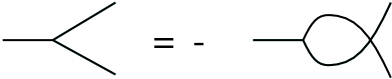
Figure 1: The AS Relation

Recall that the AS relation in Chern-Simons theory amounts to the anti-symmetry property of the structure constants, $f_{abc}$, of the Lie algebra, that is, $f_{abc}=-f_{acb}$, as depicted in Figure 1. On the other hand, in the Rozansky-Witten theory the “structure constant” which appears in diagrams is the completely symmetric tensor $\Omega_{IJKL}$ and so the identity implied by Figure 1 appears to be violated. However, one must recall that, in reality, the vertices in the Rozansky-Witten theory are connected to Grassmann odd objects and that if one thinks of the vertices as incorporating this Grassmann character then the vertex obeys the AS relation. So for example in the Rozansky-Witten theory, any diagram which has a loop centered at a vertex, as shown in Figure 2, vanishes which is a fact completely consistent with the AS relation. The reason it vanishes is that while $\Omega$ is symmetric, the labels in the loop are contracted by $\epsilon^{IJ}$ which is anti-symmetric and that the contraction is anti-symmetric is due to the fact that we had Grassmann odd variables there.

Figure 2: The Tadpole Diagram

In section 6.1 we will be quite explicit about how the AS relation arises for $b_{1}(M)=3$.

For all the similarity there is one important difference between the two theories. The vertex in the Rozansky-Witten model carries a Grassmann odd harmonic mode, $\eta^{I}_{0}$. This means that this vertex may never appear more than $2n$ times in any diagram. Thus there is a cut-off built into the perturbative expansion of the Rozansky-Witten theory.

4.4 Compact and non-Compact $X$

The spaces $X_{G}$ that are associated to a group $G$ really correspond to certain moduli spaces of monopoles. These spaces are hyper-Kähler but non-compact. Nevertheless, they are asymptotically flat. The dependence that one finds on $X_{G}$ is through terms of the form

$$\int_{X_{G}}\mathop{\mbox{Tr}}\nolimits\left(\frac{{\mathrm{R}(X_{G})}}{2\pi}\right)^{2j_{1}}\dots\,\mathop{\mbox{Tr}}\nolimits\left(\frac{{\mathrm{R}(X_{G})}}{2\pi}\right)^{2j_{n}},$$ (4.24)

with $\sum_{i}j_{i}=n$, or with explicit dependence on the holomorphic 2-form, such that the integrand is a top form. Since the manifolds are asymptotically flat integrals of this type will make sense. To be sure that the invariants do not trivially vanish we need to know if integrals of the form (4.24) are zero or not.

Non-compact hyper-Kähler manifolds abound. Examples include the Atiyah-Hitchin manifold $X_{AH}$, which is the $SU(2)$ 2-monopole moduli space as well as $T^{*}{\mathbb{C}P}^{n}$ for which Calabi [C] exhibited hyper-Kähler metrics. More generally, one has a procedure for producing examples. Suppose that one is given a hyper-Kähler manifold $X$ admitting a Lie group action of isometries $G$ which preserve the hyper-Kähler structure with $\mu:X\rightarrow\mathfrak{g}^{*}\times{\mathbb{R}}^{3}$ the corresponding moment map, where $\mathfrak{g}^{*}$ is the dual of the Lie algebra of $G$. Then, the hyper-Kähler quotient construction [HKLR] guarantees that if $G$ acts freely on $\mu^{-1}(0)$ with a Hausdorff quotient then the quotient manifold $\mu^{-1}(0)/G$ (denoted $X//G$) is once more hyper-Kähler (with the hyper-Kähler metric being the induced one). Starting with the hyper-Kähler manifold ${\mathbb{C}}^{m}\times{\mathbb{C}}^{m}$ and quotienting with various groups gives rise to many known examples of hyper-Kähler manifolds including the monopole moduli spaces of interest. For $n>1$ we are unaware of any calculations for integrals of the form (4.24). There appears to be a dearth of information on the properties of such integrals. We will proceed under the assumption that there are sufficiently many manifolds for which integrals of the type (4.24) are finite and non-vanishing.

Of course, once one has the invariants at one’s disposal, they are defined for any hyper-Kähler $X$ and not just $X_{G}$. So that, in particular, one may also consider compact manifolds. However, while non-compact hyper-Kähler manifolds are plentiful the compact variety are rare birds indeed. There are essentially two series of examples [Be]. The first is made up of a resolution of the n-fold symmetric product of $K3$ surfaces and is denoted by $S^{[n]}$. The Douady space, $S^{[n]}$, is a (real) $4n$ dimensional irreducible hyper-Kähler manifold. The second series, denoted by $K_{n}$, is related to the Douady space, $T^{[n]}$, of the n-fold symmetric product of the four dimensional torus $T$. $T^{[n]}$ is not irreducible while $K_{n}$ is. There is only one known example which is neither of type $S^{[n]}$ or $K_{n}$.

What we would really like is to get a handle on integrals of the form (4.24). Fortunately, very recently, computations of the even Chern numbers for the $S^{[n]}$ series have been made for $n=1,\dots,7$. It is quite remarkable that these are all non-zero and positive. One can check to see that the Chern characters of the tangent bundle in these cases do not vanish. As far as we are aware there are no similar computations available for the $K_{n}$ series except for the Euler characteristic, which is again strictly positive and again due to L. Göttsche [G].

4.5 Product Groups (Manifolds)

Since the Generalized Casson invariant can be morally viewed as the Euler characteristic of the moduli space of flat $G$ connections, one has immediately that the invariant for a product group is the product of the invariant of each group factor. Let the group have the form $G=G_{1}\times G_{2}$, then ${\mathrm{H}om}(\pi_{1}(M),G)/G={\mathrm{H}om}(\pi_{1}(M),G_{1})/G_{1}\times{\mathrm{H}om}(\pi_{1}(M),G_{2})/G_{2}$, or ${\mathcal{M}}(G)={\mathcal{M}}(G_{1})\times{\mathcal{M}}(G_{2})$ and consequently $\chi({\mathcal{M}}(G))=\chi({\mathcal{M}}(G_{1}))\,.\,\chi({\mathcal{M}}(G_{2}))$.

How does the Rozansky-Witten invariant behave when we consider product groups? The answer is that it factorizes as it should. To pass from the gauge theory to the sigma model one uses the dictionary $G\rightarrow X_{G}$, which for products reads $G_{1}\times G_{2}\rightarrow X_{G_{1}}\times X_{G_{2}}$. The hyper-Kähler structure of a product manifold is the natural product hyper-Kähler structure. The path integral factorizes since the space of maps factorizes and the Lagrangians split into the sum of two pieces, one of which only involves objects associated with $X_{G_{1}}$, the other involving objects only depending on $X_{G_{2}}$. We have then that

$$Z_{X_{1}\times X_{2}}^{RW}[M]=Z_{X_{1}}^{RW}[M]\,.\,Z_{X_{2}}^{RW}[M].$$ (4.25)

This simple observation has immediate consequences for the invariant, if the dependence on $X$ is only through characteristic classes. For, if this is the case, then we may expand the partition function as

$$Z_{X}^{RW}[M]=\int_{X}\sum_{j_{1}\geq\dots\geq j_{n}}^{n}\,\mathop{\mbox{Tr}}\nolimits\left(\frac{{\mathrm{R}(X)}}{2\pi}\right)^{2j_{1}}\dots\,\mathop{\mbox{Tr}}\nolimits\left(\frac{{\mathrm{R}(X)}}{2\pi}\right)^{2j_{n}}\,I_{(j_{1},\dots,j_{n})}^{n}(M).$$ (4.26)

(It is understood that in (4.26) one picks out the form of degree $4n$ in the integrand, that is $\sum_{k=1}^{n}j_{k}=n$. The actual form of the integrals $I^{n}_{j_{1},\dots,j_{n}}(M)$ depends very much on the first Betti number of $M$.) Now the factorization property (4.25) implies that, in fact,

$$Z_{X}^{RW}[M]=\int_{X}\,\mbox{e}^{\,\textstyle\sum_{j=1}^{n}\mathop{\mbox{Tr}}\nolimits\left(\frac{{\mathrm{R}}(X)}{2\pi}\right)^{2j}\,I_{j}(M)},$$ (4.27)

where

$$I_{j}(M)=I^{j}_{(j,0,\dots,0)}(M).$$ (4.28)

Consequently, the $I_{(j_{1},\dots,j_{n})}^{n}(M)$ are completely determined by the $I_{j}(M)$ for $j\leq n$. This has quite drastic implications. Since at any $n$ we are claiming that there is only one new integral $I_{n}(M)$ that arises, there is then only at most one new invariant at the given $n$. Consequently there are only, maximally, a ${\mathbb{Z}}$’s worth of invariants! We will see, in the following sections, that if $M$ has rank $\geq 1$ then both the hypothesis that $X$ enters only through its Chern numbers and the conclusions drawn hold.

The interesting case then is $b_{1}(M)=0$. In this case we cannot show that the $X$ only enters through its Chern numbers. This is just as well since it is believed that the number of LMO invariants grows rather more rapidly than linearly with dimension (degree). However, for $n=1$, Rozansky and Witten showed that the invariant is proportional to $\mathop{\mbox{Tr}}\nolimits R^{2}$ and one can also show that the double theta at $n=2$

Figure 3: The Double Theta Diagram

is proportional to $\mathop{\mbox{Tr}}\nolimits R^{4}$. Since the Mercedes Benz diagram

Figure 4: The Mercedes Benz Diagram

is proportional to the double theta this means that also at $n=2$ there is only one new invariant.

While the main thrust of our physical computations is to avoid working directly with diagrams, one aspect of the factorization property for any $M$ is very simple to describe in terms of the diagrammatic expansion. One deduces from (4.25) that for product manifolds the connected diagrams vanish while the product diagrams factor to reproduce the formula. The vanishing of the connected diagrams is a simple consequence that one gets from considering how the $\eta^{I}$ zero modes enter into the diagram.

On a product manifold, $X=X_{1}\times X_{2}$, with ${\mathrm{d}im}_{{\mathbb{R}}}X_{1}=4n_{1}$, ${\mathrm{d}im}_{{\mathbb{R}}}X_{2}=4n_{2}$ and $n_{1}+n_{2}=n$, the 2-form $\epsilon_{IJ}$ becomes the sum of the holomorphic symplectic 2-forms of each factor, i.e. $\epsilon_{IJ}=\epsilon_{IJ}^{1}+\epsilon_{IJ}^{2}$. Likewise, the curvature tensor splits as $\Omega_{IJKL}=\Omega_{IJKL}^{1}+\Omega_{IJKL}^{2}$. However, one must remember that in diagrams the curvatures are connected by $\epsilon^{IJ}$ (coming from propagators). Which means that vertices with $\Omega_{IJKL}^{1}$ assigned to them can only be connected to other vertices with $\Omega_{IJKL}^{1}$ assigned to them since the $\epsilon^{IJ}$ do not ‘mix’ manifolds. This, in turn, means that for connected diagrams one has assigned $\Omega_{IJKL}^{1}$ to every vertex or one has assigned $\Omega_{IJKL}^{2}$ to every vertex. There are $2n_{1}$ harmonic $\eta^{I}$ modes, denoted $\eta^{I}_{1}$, from $X_{1}$ and $2n_{2}$ harmonic $\eta^{I}$ modes, denoted $\eta^{I}_{2}$, from $X_{2}$.

Hence, in any given connected diagram with $m$ vertices one has exactly $m$ $\eta^{I}_{1}$ or $m$ $\eta^{I}_{2}$ zero modes appearing. In order to get a non-vanishing answer for the integral over the harmonic modes the product of connected diagrams appearing in one Feynman diagram must be such that exactly $2n_{1}$ vertices can have $\Omega_{IJKL}^{1}$ assigned to them and $2n_{2}$ vertices can have $\Omega_{IJKL}^{2}$ assigned to them. For a completely connected Feynman diagram, with $2n$ vertices, this is not possible if both $n_{1}$ and $n_{2}$ are non-zero.

4.6 Observables and $Q$-cohomology

There are a number of observables that can be defined. The expectation value of each of these is potentially a new invariant, though, as we will see, they may be invariants that we have already encountered.

For us, the basic set of observables involves powers of the holomorphic symplectic 2-form $\epsilon$, taken at some point of $M$ by pull-back. However as will be seen below, the precise point on $M$ at which the form is evaluated is immaterial and therefore will be suppressed from the notation. Let

$${\mathcal{O}}(k)=d_{k}\left(-\frac{1}{2}\eta^{I}\epsilon_{IJ}\eta^{J}\right)^{k}.$$ (4.30)

The coefficients $d_{k}$ will be fixed below. The invariants of the manifold $M$ are defined by a path integral which has an insertion of ${\mathcal{O}}(k)$, that is

$$Z^{RW}_{X}[M,{\mathcal{O}}(k)]=\int D\phi D\eta D\chi\,\mbox{e}^{\,\textstyle-S}\,{\mathcal{O}}(k).$$ (4.31)

Let $<A>$ denotes the expectation value of $A$, with respect to some set of fields $\Phi$ and some action $S(\Phi)$,

$$<A>=\int D\Phi\,\mbox{e}^{\,\textstyle-S(\Phi)}\,A.$$ (4.32)

The measure on the harmonic $\eta^{I}$ modes is determined by

$$<\eta^{I_{1}}\,\dots\,\eta^{I_{2n}}>=\epsilon^{I_{1}\,\dots\,I_{2n}},$$ (4.33)

where we mean that one integrates only over the harmonic $\eta^{I}$ modes and for which the action is taken to be zero.

We, partially, fix the coefficients $d_{k}$ by demanding that

$$d_{0}=1,$$ (4.34)

and that

$$\frac{1}{(2\pi)^{2n}}\int_{X}\sqrt{g}\,d^{4n}\phi_{0}\,<{\mathcal{O}}(k){\mathcal{O}}(n-k)>=1,$$ (4.35)

where $\sqrt{g}\,d^{4n}\phi_{0}$ is the Riemannian measure on $X$. Notice that when ${\mathrm{d}im}_{{\mathbb{R}}}X=4$, that this specifies the value of $d_{1}$, while for ${\mathrm{d}im}_{{\mathbb{R}}}X=8$, $d_{0}$, and $d_{2}$ are determined and $d_{1}$ is fixed up to a sign.

One of the most important properties of this class of observables is that

$$\int D\phi D\eta D\chi\mbox{e}^{\,\textstyle-S}\;{\mathcal{O}}(n)=\left(|H_{1}(M,{\mathbb{Z}})|\right)^{n}.$$ (4.36)

This follows from the normalization that we have chosen in (4.35) as well as the observation in [RW] that the Ray-Singer torsion provides a natural volume form which includes the Riemannian volume of $X$ times $|H_{1}(M,{\mathbb{Z}})|^{\prime}=|{\mathrm{T}or}H_{1}(M,{\mathbb{Z}})|$. The reason that it is $|H_{1}(M,{\mathbb{Z}})|$ rather than $|H_{1}(M,{\mathbb{Z}})|^{\prime}$ that appears in (4.36) is that the observables, ${\mathcal{O}}(k)$, vanish for manifolds that are not ${\mathbb{Q}}{\mathrm{H}S}$’s (this follows by a count of vertices similar to those made in section 5).

We can take the coefficients $d_{k}$, to be

$$d_{k}=\frac{(2\pi)^{2k}}{\left({\mathrm{V}ol}(X)n!\right)^{k/n}}=\left(d_{n}\right)^{k/n},$$ (4.37)

so that the observables enjoy the following property

$${\mathcal{O}}(p){\mathcal{O}}(q)={\mathcal{O}}(p+q).$$ (4.38)

We should explain why these are good operators to consider in the theory. Let ${\cal O}(\omega)$ be defined by

$${\cal O}(\omega)=\omega_{I_{1}\dots I_{k}}\,\eta^{I_{1}}\dots\eta^{I_{k}}$$ (4.39)

where the $\omega_{I_{1}\dots I_{k}}$ are both the components of a $\partial$ closed $(k,0)$ form as well as being the components of a $\overline{\partial}$ closed $(0,k)$ form. (Here $\partial$ and $\overline{\partial}$ are the holomorphic and anti-holomorphic Dolbeault operators on $X$ and the correspondence is given by the isomorphism between $TX^{(1,0)}$ and $TX^{(0,1)}$.) In equations this means that we want

$$\partial_{I}\,\omega_{I_{1}\dots I_{k}}dz^{I}dz^{I_{1}}\dots dz^{I_{k}}=0,$$ (4.40)

and

$$\overline{\partial}_{\overline{I}}\,\omega_{\overline{I}_{1}\dots\overline{I}_{k}}d\bar{z}^{\overline{I}}d\bar{z}^{\overline{I}_{1}}\dots d\bar{z}^{\overline{I}_{k}}=0,$$ (4.41)

where

$$\omega_{\overline{I}_{1}\dots\overline{I}_{k}}=\omega_{I_{1}\dots I_{k}}\,T^{I_{1}}_{\;\overline{I}_{1}}\dots T^{I_{k}}_{\;\overline{I}_{k}},$$ (4.42)

and $T^{I}_{\;\overline{I}}=g_{\overline{I}J}\epsilon^{JI}$ (see the appendix for more details about hyper-Kähler manifolds and for our conventions).

The important property of such operators is that they are both $Q$ and $\overline{Q}$ closed. That is,

$$Q\,{\cal O}(\omega) = Q\phi^{i}\,\frac{\partial{\cal O}(\omega)}{\partial\phi^{i}}$$ (4.43)

$$= \eta^{I}\,\partial_{I}\omega_{I_{1}\dots I_{k}}\,\eta^{I_{1}}\dots\eta^{I_{k}}$$

$$= 0,$$

where the third equality follows from the fact that $\omega$ is $\partial$ closed. (While these operators are $Q$ closed they are not $Q$ exact, if $\omega$ is non-trivial in cohomology, since $Q$ exactness would imply $\partial$ exactness of $\omega$.) Similarly

$$\overline{Q}\,{\mathcal{O}}(\omega) = T^{\bar{J}}_{\;J}\eta^{J}\,\partial_{\bar{J}}{\mathcal{O}}(\omega)$$ (4.44)

$$= \eta^{I}\,\partial_{I}\omega_{I_{1}\dots I_{k}}\,\eta^{I_{1}}\dots\eta^{I_{k}}$$

$$= 0,$$

Another important property of such observables is that they are essentially $d$ closed as well, where $d$ is the exterior derivative on $M$. Here essentially means that this holds because the path integral is concentrated along the constant maps. But since the dependence of the observables on $M$ is via pullback with respect to $\phi$, they do not depend on the point at which they sit on $M$.

5 Outline of the Proof of Heuristic Theorem 2.

The strategy of the proof will be to decide which types of Feynman diagrams can contribute and then to find a way of encoding all the relevant information without doing any expansions. The one piece of information that we will use continuously is that, on expanding out the interaction part of the action, the interaction terms will be of the form

$$V_{1}^{p}\,V_{2}^{q},$$ (5.1)

where

$$V_{1} = \frac{1}{6}\int_{M}\Omega_{IJKL}(\phi_{0})\chi^{I}\chi^{J}\chi^{K}\eta^{L}_{0}$$ (5.2)

$$V_{2} = -\int_{M}\Omega_{IJKL}(\phi_{0})T^{J}_{\,\overline{M}}\chi^{I}\,\eta^{L}_{0}\phi^{\overline{M}}_{\perp}\,*d\phi^{K}_{\perp}.$$ (5.3)

There is a condition on the number of interactions that arise from the fact that both vertices $V_{1}$ and $V_{2}$ are linear in $\eta^{I}_{0}$, which we recall is constant on $M$. Since $\eta^{I}_{0}$ is constant on $M$, this means that the “path integral” over this “field” is actually a 2n-fold product of Berezin integrals (the exact specification of the measure is described in appendix B). Furthermore, from the rules that we describe for such variables, we see that the integration will vanish identically unless the integrand includes the product of all $2n$ components of $\eta^{I}_{0}$ (each occuring exactly once). Consequently one has

$$p+q=2n.$$ (5.4)

The rest of the proof depends on how many $\chi^{I}$ harmonic modes there are. The importance of these modes lies in the fact that, like the $\eta^{I}_{0}$, they will only appear in the vertices. Hence, for the same reason as for the harmonic $\eta^{I}$, the path integral will vanish identically unless the integrand includes the product of all the harmonic components of $\chi^{I}$. The number of harmonic modes of $\chi^{I}$ is $2nb_{1}(M)$. This means that there is another condition that must be satisfied to ensure that the integral has a chance of not vanishing, which is

$$3p+q\geq 2nb_{1}(M).$$ (5.5)

This inequality comes by noticing that if $3p+q<2nb_{1}(M)$ then certainly the integrand will not have the required product of harmonic $\chi^{I}$. As the constraint (5.5) depends on $b_{1}(M)$, we go through the possible $b_{1}(M)$ values and along the way we will strengthen it. Subtracting (5.4) from (5.5) gives the constraint

$$p\geq n(b_{1}(M)-1).$$ (5.6)

5.1 Manifolds with $b_{1}(M)\geq 4$

From (5.6) we see that if $b_{1}(M)\geq 4$, then clearly $p>2n$, but then (5.4) certainly cannot be satisfied. Consequently, we see that it is in fact impossible to integrate up the harmonic modes of $\chi^{I}$ and hence the Rozansky-Witten path integral vanishes.

6 Manifolds with $b_{1}(M)=3$

The inequality (5.6) says, for $b_{1}(M)=3$, that $p\geq 2n$ and this intersects with (5.4) only if $p=2n$ and $q=0$. This condition tells us that we are to ignore $V_{2}$ completely, so that perturbatively one is interested in

$$V_{1}^{2n}.$$ (6.1)

However, we know more. Since there are $6n$ $\chi^{I}$ harmonic modes, all the $\chi^{I}$ appearing in (6.1) must be harmonic. This means that vertex $V_{1}$ effectively reduces to

$$V_{1}=\frac{1}{6}\int_{M}\,\Omega_{IJKL}(\phi_{0})\chi^{I}_{0}\chi^{J}_{0}\chi^{K}_{0}\eta^{L}_{0}$$ (6.2)

and in turn that the Lagrangians (4.14, 4.15) reduces (with a slight rearrangement) to

$$L_{\perp} = \frac{1}{2}g_{ij}(\phi_{0})d\phi^{i}_{\perp}*d\phi^{j}_{\perp}+\epsilon_{IJ}(\phi_{0})\chi^{I}_{\perp}*d\eta^{J}_{\perp}+\frac{1}{2}\epsilon_{IJ}(\phi_{0})\chi^{I}_{\perp}d\chi^{J}_{\perp}$$ (6.3)

$$L_{0} = \frac{1}{6}\Omega_{IJKL}(\phi_{0})\chi^{I}_{0}\chi^{J}_{0}\chi^{K}_{0}\eta^{L}_{0}$$ (6.4)

where a zero subscript indicates the field is harmonic while the $\perp$ subscript indicates that the field is orthogonal to the harmonic modes on $M$. The path integral to be performed is, symbolically,

$$\int d\Phi_{0}\;\mbox{e}^{\,\textstyle-\int_{M}L_{0}}\;\int D\Phi_{\perp}\;\mbox{e}^{\,\textstyle-\int_{M}\,L_{\perp}},$$ (6.5)

where $\Phi$ denotes the set of fields. Rozansky and Witten [RW] have shown that

$$\int D\Phi_{\perp}\;\mbox{e}^{\,\textstyle-\int_{M}\,L_{\perp}}=\left(|{\mathrm{H}}_{1}(M,{\mathbb{Z}})|^{\prime}\right)^{n},$$ (6.6)

where $|{\mathrm{H}}_{1}(M,{\mathbb{Z}})|^{\prime}$ is the order of ${\mathrm{T}or\,H}_{1}(M,{\mathbb{Z}})$. Consequently, the Rozansky-Witten invariant in this case has the very succinct representation

$$Z^{RW}_{X}[M]=\left(|{\mathrm{H}}_{1}(M,{\mathbb{Z}})|^{\prime}\right)^{n}\int d\Phi_{0}\;\mbox{e}^{\,\textstyle-\int_{M}L_{0}}.$$ (6.7)

Let $\omega^{\alpha}$, $\alpha=1,\,2,\,3$ be a basis of $H^{1}(M,{\mathbb{Z}})$. Since $\chi_{0}^{I}$ is harmonic on $M$, we see that it must have the expansion $\chi_{0}^{I}=\chi^{I}_{\alpha}\omega^{\alpha}$, where the coefficients $\chi^{I}_{\alpha}$, for each $\alpha=1,2,3$, are generators of $\wedge\phi^{*}T^{(1,0)}X$. Substitution of this expansion in (6.2) gives

$$V_{1} = \frac{1}{6}\Omega_{IJKL}(\phi_{0})\chi^{I}_{\alpha}\chi^{J}_{\beta}\chi^{K}_{\gamma}\eta^{L}_{0}\int_{M}\,\omega^{\alpha}\omega^{\beta}\omega^{\gamma}$$ (6.8)

$$= \frac{1}{6}\Omega_{IJKL}(\phi_{0})\chi^{I}_{\alpha}\chi^{J}_{\beta}\chi^{K}_{\gamma}\eta^{L}_{0}\epsilon^{\alpha\beta\gamma}\;I(M),$$

where

$$I(M)=\frac{1}{6}\epsilon_{\alpha\beta\gamma}\int_{M}\,\omega^{\alpha}\omega^{\beta}\omega^{\gamma}.$$ (6.9)

By the arguments that we presented at the start of this section culminating in (6.1) we immediately have that the Rozansky-Witten invariant is proportional to $I(M)^{2n}$.

To determine the coefficient, it suffices to compute the invariant for any 3-manifold of rank 3 as it does not depend on $M$ but only on $X$. In [T] (equation (3.23)), the second author showed that the Rozansky-Witten invariant for the 3-torus, $T^{3}$, is equal to the Euler characteristic of $X$ if it is compact. (More generally, it is equal to the integral of the Euler form over $X$) Denote this (in both cases) by ${\mathbf{e}}(X)$. We also have $I(T^{3})^{2}=1$ so that we find for manifolds $M$, with $b_{1}(M)=3$,

$$Z^{RW}_{X}[M]={\mathbf{e}}(X)\left(|H_{1}(M,{\mathbb{Z}})|^{\prime}I(M)^{2}\right)^{n}.$$ (6.10)

One may relate this back to the Lescop invariant $\lambda(M)$, as

$$I(M)^{2}=\frac{\lambda(M)}{|H_{1}(M,{\mathbb{Z}})|^{\prime}}$$ (6.11)

so that

$$Z^{RW}_{X}[M]=c_{X}\lambda(M)^{n},$$ (6.12)

where

$$c_{X}={\mathbf{e}}(X).$$ (6.13)

One can also get this result by performing the finite dimensional integrals that were left to be done in (6.7). Indeed these are computed directly from (B.38).

As already explained in section 4.4 there are compact and non-compact $X$ for which ${\mathbf{e}}(X)$ is non-vanishing for every $n$, so that (6.12) is not empty. For example, for the $S^{[n]}$ series one has the generating function

$$\sum_{n=0}^{\infty}{\mathbf{e}}(S^{[n]})t^{n}=\prod_{k=1}^{\infty}\frac{1}{\left(1-t^{k}\right)^{24}},$$ (6.14)

while for the $K_{n}$ series one has

$${\mathbf{e}}(K_{n})=(n+1)^{3}\sigma_{1}(n+1),$$ (6.15)

where $\sigma_{1}(n)$ is the sum of the divisors of $n$. It is amusing that, for $S^{[n]}$, if one replaces the Casson invariant with the indeterminant $t$, then summing over $n$ in (6.12) reproduces the generating function for the Euler characteristics (6.14).

On the non-compact side $\left(X_{AH}\right)^{n}$ will do, since ${\mathbf{e}}(X_{AH}^{n})={\mathbf{e}}(X_{AH})^{n}=1$.

6.1 The AS Relation

The vertex with the $\chi$ zero modes attached is

$$V_{1}=\frac{1}{6}\Omega_{IJKL}(\phi_{0})\chi^{I}_{\alpha}\chi^{J}_{\beta}\chi^{K}_{\gamma}\eta^{L}_{0}\int_{M}\,\omega^{\alpha}\omega^{\beta}\omega^{\gamma}.$$ (6.16)

If one extracts the part that depends on $X$ from the dependence on $M$ we can write the vertex as

$$V_{1}=F_{\alpha\beta\gamma}(X)\,\int_{M}\,\omega^{\alpha}\omega^{\beta}\omega^{\gamma},$$ (6.17)

where $F_{\alpha\beta\gamma}(X)=\frac{1}{6}\Omega_{IJKL}(\phi_{0})\chi^{I}_{\alpha}\chi^{J}_{\beta}\chi^{K}_{\gamma}\eta^{L}_{0}$, is totally antisymmetric in its three labels. Consequently, it is the vertex $F_{\alpha\beta\gamma}(X)$ that satisfies the AS relation. In Chern-Simons theory a similar vertex arises when one replaces the gauge connection with harmonic modes in the cubic term, that is, one sets $A^{a}=A^{a}_{\alpha}\omega^{\alpha}$. The cubic term is now proportional to $K_{\alpha\beta\gamma}(G)\,\int_{M}\,\omega^{\alpha}\omega^{\beta}\omega^{\gamma}$, where $K_{\alpha\beta\gamma}(G)=f_{abc}A^{a}_{\alpha}A^{b}_{\beta}A^{c}_{\gamma}$. Notice that $K_{\alpha\beta\gamma}(G)$ is also antisymmetric in its three labels. The antisymmetry of $F_{\alpha\beta\gamma}(X)$ is a consequence of the symmetry of $\Omega$ and the anticommuting properties of the Grassmann variables $\chi^{I}_{\alpha}$. The antisymmetry of $K_{\alpha\beta\gamma}(G)$ rests on the antisymmetry of the structure constants of $G$, $f_{abc}$ and the fact that the variables $A^{a}_{\alpha}$ commute with each other.

7 Manifolds with $b_{1}(M)=2$

In this case from (5.6) we learn that $p\geq n$. However, we can show that $q=0$. To see this, note that in the vertex $V_{1}$ there can be at most two harmonic $\chi^{I}$, since the wedge product of three would be zero ($b_{1}(M)=2$). This means that we can refine (5.5) to obtain the inequality

$$2p+q\geq 4n$$ (7.1)

which together on subtracting (5.4) tells us that $p\geq 2n$. Hence, once more we find that $p=2n$ and $q=0$. What this means for us is that we may ignore $V_{2}$ and also in order to guarantee that the harmonic modes are accounted for, two and only two of the $\chi^{I}$ appearing in $V_{1}$ must be harmonic. One sets

$$V_{1}=\frac{1}{2}\int_{M}\,\Omega_{IJKL}(\phi_{0})\chi^{I}_{\perp}\chi^{J}_{0}\chi^{K}_{0}\eta^{L}_{0}.$$ (7.2)

Let $\omega^{\alpha}$, $\alpha=1,\,2$, be a basis of $H^{1}(M,{\mathbb{Z}})$. Since $\chi_{0}^{I}$ is harmonic on $M$, we see that it must have the expansion $\chi_{0}^{I}=\chi^{I}_{\alpha}\omega^{\alpha}$, where the coefficients $\chi^{I}_{\alpha}$, for each $\alpha=1,2$, are generators of $\wedge\phi^{*}T^{(1,0)}X$. Inserting this into (7.2), yields

$$V_{1}=-\frac{1}{2}\Omega_{IJKL}(\phi_{0})\chi^{J}_{\alpha}\chi^{K}_{\beta}\eta^{L}_{0}\int_{M}\,\chi^{I}_{\perp}\omega^{\alpha}\omega^{\beta}.$$ (7.3)

While the wedge product $\omega^{\alpha}\wedge\omega^{\beta}$ is exact it is not harmonic. Set $\omega^{\alpha}\wedge\omega^{\beta}=\epsilon^{\alpha\beta}\,dg$, where $g$ is a one form on $M$. $g$ is only defined up to exact pieces so to be definite we demand that $d*g=0$.

The actions become,

$$\int_{M}L_{1} = \int_{M}\,\left(\frac{1}{2}g_{ij}(\phi_{0})d\phi^{i}_{\perp}*d\phi^{j}_{\perp}+\epsilon_{IJ}(\phi_{0})\chi^{I}_{\perp}*d\eta^{J}_{\perp}\right)$$ (7.4)

$$\int_{M}L_{2} = \frac{1}{2}\epsilon_{IJ}(\phi_{0})\int_{M}\chi^{I}_{\perp}d\chi^{J}_{\perp}-\Lambda_{I}\int_{M}\,d\chi^{I}_{\perp}\,g.$$ (7.5)

where we have set $\Lambda_{I}=\frac{1}{2}\Omega_{IJKL}(\phi_{0})\epsilon^{\alpha\beta}\chi^{J}_{\alpha}\chi^{K}_{\beta}\eta^{L}_{0}$.

We now complete the square

$$\int_{M}L_{2}=\frac{1}{2}\epsilon_{IJ}(\phi_{0})\int_{M}\left(\chi^{I}_{\perp}+\epsilon^{IK}\Lambda_{K}g\right)d\left(\chi^{J}_{\perp}+\epsilon^{JL}\Lambda_{L}g\right)+\frac{1}{2}\Lambda_{I}\epsilon^{IJ}\Lambda_{J}\int_{M}gdg.$$ (7.6)

Notice also that the part of (7.4) that involves $\chi_{\perp}^{I}$ is

$$\int_{M}\epsilon_{IJ}(\phi_{0})\chi^{I}_{\perp}*d\eta^{J}_{\perp}=\int_{M}\epsilon_{IJ}(\phi_{0})\left(\chi^{I}_{\perp}+\epsilon^{IK}\Lambda_{K}g\right)*d\eta^{J}_{\perp},$$ (7.7)

since we have chosen $d*g=0$. We now change variables in the path integral. Since $\chi^{I}_{\perp}$ only appears in the action in the combination $\hat{\chi}^{I}_{\perp}=\chi^{I}_{\perp}+\epsilon^{IK}\Lambda_{K}\,g$, we change variables to $\hat{\chi}^{I}_{\perp}$. Does such a change of variables make sense? The answer is yes. Firstly, since $\Lambda_{I}$ is Grassmann odd we are maintaining the grading of the fields. Secondly, $g$ lives in $H^{1}_{\perp}(M)$ so this character of the field is also preserved. Lastly, the Jacobian for such a change of variables is unity since the object by which we are shifting $\chi^{I}_{\perp}$ does not depend on $\chi^{I}_{\perp}$.

Hence the actions (7.4) and (7.5) can be grouped as follows

$$S_{0}+S_{\perp}=\int_{M}\left(L_{1}+L_{2}\right)$$ (7.8)

where

$$S_{0} = \frac{1}{2}\Lambda_{I}\epsilon^{IJ}\Lambda_{J}\int_{M}gdg,$$ (7.9)

$$S_{\perp} = \int_{M}\,\left(\frac{1}{2}g_{ij}(\phi_{0})d\phi^{i}_{\perp}*d\phi^{j}_{\perp}\right.$$ (7.10)

$$\;\;\;+\left.\frac{1}{2}\epsilon_{IJ}(\phi_{0})\int_{M}\hat{\chi}^{I}_{\perp}d\hat{\chi}^{J}_{\perp}+\epsilon_{IJ}(\phi_{0})\hat{\chi}^{I}_{\perp}*d\eta^{J}_{\perp}\right).$$

This shows us, once more, that the path integral over all the fields splits nicely as,

$$\int d\Phi_{0}\;\mbox{e}^{\,\textstyle-S_{0}}\;\int D\Phi_{\perp}\;\mbox{e}^{\,\textstyle-S_{\perp}}.$$ (7.11)

The path integral,

$$Z_{{\perp}}=\int D\Phi_{\perp}\;\mbox{e}^{\,\textstyle S_{\perp}},$$ (7.12)

is essentially the same one that was discussed in the rank 3 case so it gives a factor of

$$\left(|{\mathrm{H}}_{1}(M,{\mathbb{Z}})|^{\prime}\right)^{n}.$$ (7.13)

It is the first factor that is of interest,

$$Z_{0}=\int d\Phi_{0}\;\mbox{e}^{\,\textstyle-S_{0}}.$$ (7.14)

The integral $\mu(M)=\int_{M}gdg$, is a well-known invariant of the manifold $M$ (see [L] for the Poincaré dual linking number definition). The Casson invariant in this case is $-|{\mathrm{H}}_{1}(M,{\mathbb{Z}})|^{\prime}\,\mu(M)$.

We have then that

$$Z_{X}^{RW}[M]=c^{\prime}_{X}\left(\lambda_{M}\right)^{n},$$ (7.15)

where,

$$c_{X}^{\prime}=\int d\Phi_{0}\,\frac{\left(\Lambda_{I}\epsilon^{IJ}\Lambda_{J}\right)^{n}}{2^{n}n!}.$$ (7.16)

Below, we will establish that $c_{X}^{\prime}=c_{X}$.

7.1 On the Relationship with [BeHa]

In [BeHa] the LMO invariant and the Lescop invariant for manifolds with $b_{1}(M)=2$ were related. These authors established that the coefficients of the powers of the Lescop invariant are related to evaluations of certain diagrams that we can refer to as ${\mathbf{H}}$ diagrams. One should, as we have previously seen, think of the vertices in the Rozansky-Witten theory as if they are 3-point vertices, the $\eta^{I}_{0}$ leg being thought of as the ‘coupling constant’ (i.e. one focuses on the order of the $\eta^{I}_{0}$ in the expansion). This 3-point vertex,

$$V_{IJK}^{3}\,\chi^{I}_{1}\chi^{J}_{2}\chi^{K}_{3}=\frac{1}{6}\,\Omega_{IJKL}\,\chi^{I}_{\alpha}\chi^{J}_{\beta}\chi^{K}_{\gamma}\,\eta^{L}_{0}\,\epsilon^{\alpha\beta\gamma},$$ (7.17)

is what appears finally in (6.7) in the rank 3 case. Ignoring the $\eta^{I}_{0}$, we see that the vertex carries $3$ legs which are attached to the three $\chi_{\alpha}^{I}$ zero modes. Each of the legs carries a different value of $\alpha=1,2,3$. In the current situation, however, we find in the exponent not a 3-point vertex but rather a 4-point vertex (which is quadratic in the coupling constant)

$$V^{4}_{IJKL}\,\chi^{I}_{1}\chi^{J}_{2}\chi^{K}_{1}\chi^{L}_{2}=\frac{1}{2}\Lambda_{I}\,\epsilon^{IJ}\Lambda_{J}.$$ (7.18)

This vertex is the ${\mathbf{H}}$ diagram. The vertex is really a join of two 3-point vertices along the leg marked 3. The external legs can only carry the labels $1,2$.

We note that there is another way of expressing the integrals that still need to be performed and which exhibits very clearly that the 4-point vertex comes from the join of 3-point vertices. Introduce another Grassmann odd variable $\psi^{I}$. Then we have

$$\int d\mu(\psi)\,\mbox{e}^{\,\textstyle\left(-\frac{1}{2}\psi^{I}\epsilon_{IJ}\psi^{J}+a\Lambda_{I}\psi^{I}\right)}=\mbox{e}^{\,\textstyle\left(-\frac{1}{2}a^{2}\Lambda_{I}\epsilon^{IJ}\Lambda_{J}\right)}.$$ (7.19)

In this way it is as if we have an extra $\chi$ harmonic mode, that is $\psi^{I}$ plays the role of $\chi_{3}^{I}$. The 4-point vertex then is really understood as

$$V^{4}_{IJKL}\,\chi^{I}_{1}\chi^{J}_{2}\chi^{K}_{1}\chi^{L}_{2}=\frac{1}{2}V^{3}_{I_{1}J_{1}K_{1}}\,\chi^{J_{1}}_{1}\chi^{K_{1}}_{2}\,\langle\psi^{I_{1}}\psi^{I_{2}}\rangle\,V^{3}_{I_{2}J_{2}K_{2}}\,\chi^{J_{2}}_{1}\chi^{K_{2}}_{2},$$ (7.20)

meaning a contraction of two 3-point vertices along the legs marked with a 3.

So far we have shown how the ${\mathbf{H}}$ diagrams arise in the Rozansky-Witten theory. Now we will see that this characterization of the ${\mathbf{H}}$ diagram automatically establishes that the constants $c_{X}$ for rank 3 manifolds and $c_{X}^{\prime}$ for rank 2 manifolds are equal. The expressions (7.19) look like those obtained for the rank 3 case. In fact the resemblance becomes equality with the following observation: To saturate the integral over $\eta^{I}$ one must expand the exponential,

$$\mbox{e}^{\,\textstyle a\Lambda_{I}\psi^{I}},$$ (7.21)

out to the $2n$’th term. However, in so doing we will also have $2n$ products of $\psi^{I}$, which is exactly what is required to be able to perform the $\psi^{I}$ integral. Consequently, the only term of the expansion of the exponential of the quadratic term, $\exp{(-1/2\psi^{I}\epsilon_{IJ}\psi^{J})}$, is the zeroth order piece, namely $1$.

Consequently, we have that

$$\int d\Phi_{0}\;\mbox{e}^{\,\textstyle-\frac{1}{2}\mu(M)\Lambda_{I}\epsilon^{IJ}\Lambda_{J}} = \int d\Phi_{0}\;\mbox{e}^{\,\textstyle-\sqrt{\mu(M)}\Omega_{IJKL}\psi^{I}\chi^{J}_{1}\chi^{K}_{2}\eta^{L}}$$ (7.22)

$$= \mu(M)^{n}\,{\mathbf{e}}(X),$$

where the measure on the right hand side of the first equality includes that of the $\psi^{I}$ field. Now we are done since,

$$\lambda(M)={\mathbf{e}}(X_{AH})|H_{1}(M,{\mathbb{Z}})|^{\prime}\,\mu(M),$$ (7.23)

we have shown that

$$Z_{X}^{RW}[M]=c_{X}\lambda(M)^{n}.$$ (7.24)

8 Manifolds with $b_{1}(M)=1$

When $b_{1}(M)=1$, the vertex $V_{1}$ can have at most one harmonic $\chi^{I}$. Note that in order to saturate the integral over the harmonic $\chi^{I}$ fields, there is a bound

$$p+q\geq 2n.$$ (8.1)

This bound is already implied by (5.4) and so appears to convey no new information. However, one should read it in a different way. It tells us that the equality can be met only if one of the $\chi^{I}$ that appears in the $V_{1}$ vertex and the one that appears in the $V_{2}$ vertex are harmonic. Let $\omega$ be a generator for ${\mathrm{H}}^{1}(M,{\mathbb{Z}})$ so that we may write $\chi^{I}_{0}=c^{I}\omega$, where $\omega$ satisfies $\int_{M}\omega*\omega=1$. As before, if a field appears with a $\perp$ subscript then it is orthogonal to the harmonic modes while, if it has a zero subscript then it is understood to be harmonic. We may as well set

$$L_{1} = \frac{1}{2}\left(g_{ij}\,d\phi^{i}_{\perp}*d\phi^{j}_{\perp}-\gamma_{i}^{AK}\gamma_{j}^{BL}\epsilon_{AB}\Omega_{IJKL}\chi^{I}_{0}\eta^{J}_{0}\phi^{i}_{\perp}*d\phi^{j}_{\perp}+2\epsilon_{IJ}\chi^{I}_{\perp}*d\eta^{J}_{\perp}\right)$$ (8.2)

$$= g_{I\overline{J}}d_{A}\phi^{I}_{\perp}*d\overline{\phi}^{\overline{J}}_{\perp}+\epsilon_{IJ}\chi^{I}_{\perp}*d\eta^{J}_{\perp}$$

$$L_{2} = \frac{1}{2}\left(\epsilon_{IJ}(\phi_{0})\chi^{I}_{\perp}d\chi^{J}_{\perp}+\Omega_{IJKL}\chi^{I}_{\perp}\chi^{J}_{\perp}\chi^{K}_{0}\eta^{L}_{0}\right),$$ (8.3)

$$= \frac{1}{2}\epsilon_{IJ}(\phi_{0})\chi^{I}_{\perp}d_{A}\chi^{J}_{\perp}.$$

The covariant derivative in (8.3) is defined by

$$d_{A}\chi^{J}=d\chi^{J}+A^{J}_{\,K}\chi^{K}$$ (8.4)

where the “connection” is

$$A^{I}_{\,J} = -\epsilon^{IM}(\phi_{0})\Omega_{MNJK}(\phi_{0})\chi^{N}_{0}\eta^{K}_{0}$$ (8.5)

$$= a^{I}_{\,J}\,\omega,$$ (8.6)

and

$$a^{I}_{\,J}=-\epsilon^{IM}(\phi_{0})\Omega_{MNJK}(\phi_{0})c^{N}\eta^{K}_{0}.$$ (8.7)

The connection is flat; since the tensors that appear in (8.6) depend only on the constant maps, and the fields there are also harmonic, we are assured that $dA^{I}_{\,J}=0$. Furthermore, as $A^{I}_{\,J}$ is proportional to $\omega$, we know that $A^{I}_{\,J}\wedge A^{J}_{\,K}=0$, so finally

$$F_{A}=0.$$ (8.8)

Notice that the connection (8.6) is symmetric when the labels are both down, $A_{IJ}=\epsilon_{IK}A^{K}_{\,J}=A_{JI}$, by virtue of the symmetry properties of $\Omega_{IJKL}$.

8.1 A Path Integral for Ray-Singer Torsion

We now remind the reader of how one formulates the Ray-Singer Torsion in terms of path integrals. This is a small variant on the formulation introduced by Schwarz [S]. Let $V$ be a vector bundle over $M$ with a fixed flat connection $A$. One begins with an action

$$S_{0}=\int_{M}\frac{1}{2}\epsilon_{IJ}\chi^{I}d_{A}\chi^{J}$$ (8.9)

which makes sense for any $M$ with real dimension $4k+1$ with the $\chi^{I}$ Grassmann even $2k$ forms with values in $V$ or with real dimension $4k-1$ and the $\chi^{I}$ are Grassmann odd $2k-1$ forms with values in $V$. As it stands this system is not well prescribed since

$$S_{0}(\chi^{I}+d_{A}\phi^{I})=S_{0}(\chi^{I}),$$ (8.10)

that is, the action enjoys a gauge symmetry. In general $\phi^{I}$ will be a form of one degree less than that of $\chi^{I}$. The symmetry requires that the connection be flat. Hence on the space of $\chi^{I}$, denoted by ${\mathcal{X}}$, there is an action by the gauge group ${\mathcal{G}}$ given by

$$\phi\left(\chi^{I}\right)=\chi^{I}+d_{A}\phi^{I},\;\;\;\;\;\phi\in{\mathcal{G}}.$$ (8.11)

We do not wish to integrate over ${\mathcal{X}}$ but rather over ${\mathcal{X}}/{\mathcal{G}}$. Equivalently we chose to integrate on a slice (section). In doing this one needs to compare Riemannian volumes on the section and on the space ${\mathcal{X}}$. This comparison shows that one must multiply by a volume factor, namely the Fadeev-Popov determinant. Ultimately one finds

$$\int_{{\mathcal{X}}/{\mathcal{G}}}\mbox{e}^{\,\textstyle-S_{0}}=\int_{{\mathcal{X}}}\mbox{e}^{\,\textstyle-S_{0}}\,\delta\left(s\right)\,\Delta_{{\mathrm{F}P}},$$ (8.12)

where $s$ denotes the section of choice.

Typically one takes the section to be

$$s^{I}=d_{A}*\chi^{I},$$ (8.13)

since, with respect to the metric on $M$, it projects along the direction of gauge transformations. The path integral with this choice of gauge is

$$\int_{{\mathcal{X}}/{\mathcal{G}}}\mbox{e}^{\,\textstyle-S_{0}}=\int_{{\mathcal{X}}}D\eta^{I}D\phi^{I}D\phi^{\overline{I}}\mbox{e}^{\,\textstyle-S_{a}},$$ (8.14)

where

$$S_{a}=S_{0}+\int_{M}\epsilon_{IJ}\eta^{I}d_{A}*\chi^{J}+\int_{M}\phi^{\overline{J}}d_{A}*d_{A}\phi^{I}g_{I\overline{J}}.$$ (8.15)

Notice that the path integral over $\eta^{I}$ is there to give back the delta function constraint onto the section (8.13) while the integral over $\phi^{i}$ reproduces the Fadeev-Popov determinant.

The sum of the actions of (8.2) and (8.3),

$$S_{b}=S_{0}+\int_{M}\epsilon_{IJ}\eta^{I}d*\chi^{J}+\int_{M}\phi^{\overline{J}}d*d_{A}\phi^{I}g_{I\overline{J}}.$$ (8.16)

almost coincides with (8.15). A glance at (8.16) suggests we are quantizing the same starting action (8.9), but with a different choice of section,

$$s^{I}=d*\chi^{I}.$$ (8.17)

We would expect that the path integral would not depend on which choice of section we make use of. This is not quite true due to the presence of zero modes of the fields. The path integral that we wish to perform, with action (8.16), has the condition that we do not include an integration over the constant $\phi^{i}$ and $\eta^{I}$ modes, nor do we integrate over the harmonic part of $\chi^{I}$. However, in evaluating the path integral which gives us the Ray-Singer Torsion, no such restriction is made, since one requires the cohomology of $d_{A}$ to be acyclic (if it is not acyclic then one explicitly projects out the harmonic modes of the twisted Laplacian). The path integral that we want is then not equal to the path integral for the Ray-Singer Torsion, but rather is equal to the path integral for the Ray-Singer Torsion divided by the integration over the harmonic modes (of the usual Laplacian).

The part of the path integral (8.14) over the harmonic modes is

$$\int d\phi^{I}d\phi^{\overline{J}}d\eta^{I}dc^{I}\,\mbox{e}^{\,\textstyle-\left(\eta^{I}\epsilon_{IJ}A^{J}_{\,K}c^{K}-\phi^{\overline{J}}g_{\overline{J}I}A^{I}_{\,K}A^{K}_{\,L}\phi^{L}\right)}=\frac{\det\left(a_{IJ}\right)}{\det\left(a_{IK}a^{K}_{\,J}\right)}.$$ (8.18)

We have found then, for manifolds with $b_{1}(M)=1$, that the path integral is

$$Z_{X}^{RW}[M]=\frac{1}{(2\pi)^{2n}}\int_{X}\det(a)\left(\tau_{{\mathrm{R}S}}(a)\right)^{1/2}$$ (8.19)

where $\tau_{{\mathrm{R}S}}(a)$ is the Ray-Singer Torsion for the connection $A$ of a flat ${\mathrm{s}p}(n)$ bundle over $M$ (in the $2n$-dimensional representation). Since in the integrand we must pick a top form, one may move the $2\pi$ factors into a different position,

$$Z_{X}^{RW}[M]=\int_{X}\det(a/2\pi)\left(\tau_{{\mathrm{R}S}}(a/2\pi)\right)^{1/2}.$$ (8.20)

8.2 A BRST Argument

There is an equivalent way to express the fact that the path integral that we are interested in yields (8.19). We start with a BRST formulation of the model given by the action (8.9). The BRST symmetry in question is

$$Q\chi^{I}=d_{A}\phi^{I},\;\;Q\phi^{I}=0,\;\;Q\phi^{\overline{I}}=g^{\overline{I}J}\epsilon_{JI}\eta^{I},\;\;Q\eta^{\overline{I}}=0,$$ (8.21)

and $Q^{2}=0$. We may still decompose the fields as to whether or not they are harmonic with respect to the usual de-Rham operator $d$ so that (8.21) splits as

$$\begin{array}[]{ll}Q\chi^{I}_{\perp}=d_{A}\phi^{I}_{\perp}&Q\chi^{I}_{0}=A^{I}_{\;J}\phi^{J}_{0}\\ Q\phi^{\overline{I}}_{\perp}=g^{\overline{I}J}\epsilon_{JI}\eta^{I}_{\perp}&Q\phi^{\overline{I}}_{0}=g^{\overline{I}J}\epsilon_{JI}\eta^{I}_{0},\end{array}$$ (8.24)

and

$$Q\phi^{I}_{\perp}=0=Q\phi^{I}_{0}\;\;\;Q\eta^{I}_{\perp}=0=Q\eta^{I}_{0}.$$ (8.25)

Notice that the action (8.9) is in fact

$$S_{0}=\int_{M}\frac{1}{2}\epsilon_{IJ}\chi^{I}_{\perp}d_{A}\chi^{J}_{\perp}.$$ (8.26)

We take the holonomy of $X$ to be irreducible, which means that $A^{I}_{\;K}\phi^{K}=0$ implies that $\phi^{I}=0$. This is not really a restriction since we will not be using any special properties of the curvature 2-form in any case. So, put another way, we are considering $sp(n)$ matrices $a^{I}_{\;J}$ which are invertible. The fact that $\chi_{0}^{I}=\omega c^{I}$ makes no appearance in the action is due to the fact that it is pure gauge (that is it can be gauge transformed to zero), since

$$\omega c^{I}=d_{A}(a^{-1})^{I}_{\;J}c^{J}.$$ (8.27)

We may gauge fix in two stages. Firstly we fix the $\perp$ modes, and the gauge fixing term is taken to be

$$\{Q,\int_{M}\,g_{I\overline{J}}\chi^{I}_{\perp}*d\phi^{\overline{J}}_{\perp}\}=\int_{M}\,\left(\epsilon_{IJ}\chi^{I}_{\perp}*d\eta^{J}_{\perp}+g_{I\overline{J}}d_{A}\phi^{I}_{\perp}*d\phi^{\overline{J}}_{\perp}\right).$$ (8.28)

Up to this point we see that the path integral that we are interested in has as its action (8.26) and (8.28). However, the path integral for the Ray-Singer torsion requires that we also gauge fix the zero mode symmetry. In fact we should set $c^{I}$ to zero since, by (8.27) it is pure gauge. In order to do this we add

$$\{Q,\int_{M}\,g_{I\overline{J}}\chi^{I}_{0}*\omega\phi^{\overline{J}}_{0}\}=\left(\epsilon_{IJ}c^{I}\eta^{J}_{0}+g_{I\overline{J}}a^{I}_{\;K}\phi^{I}_{0}\,\phi^{\overline{J}}_{0}\right).$$ (8.29)

While this two step gauge fixing is not the usual covariant gauge fixing we know that, nevertheless, it leads correctly to the Ray-Singer torsion, since it differs from the covariant gauge fixing terms by a BRST exact term. Denote the path integral for the Ray-Singer torsion by $Z_{RS}$, the path integral that one gets simply by integrating over the perpendicular modes, with action (8.26) and (8.28), by $Z_{\perp}$, and the zero mode partition function by $Z_{0}$ that comes from (8.29). The path integral now nicely factors as

$$Z_{RS}=Z_{\perp}\,Z_{0},$$ (8.30)

or put another way

$$Z_{\perp}=Z_{RS}/Z_{0}=\det(a)\left(\tau_{{\mathrm{R}S}}(a)\right)^{1/2}.$$ (8.31)

8.3 Explicit Expression for the Path Integral

Since $a$ takes its values in the adjoint representation of $sp(n)$, by a global gauge transformation we may rotate it into the Cartan sub-algebra of $sp(n)$. Denote the $n$ eigenvalues of $a/2\pi$ by $x_{i}$. Then $a/2\pi$ is conjugate to ${\mathbf{d}iag}\left(x_{1},x_{2},\dots,x_{n},-x_{1},-x_{2},\dots,-x_{n}\right)$.

Set $t_{i}=\mbox{e}^{\,\textstyle x_{i}}$. Rewrite the integrand of (8.20) as

$$\det(a/2\pi)\left(\tau_{{\mathrm{R}S}}(a/2\pi)\right)^{1/2}=\prod_{i=1}^{n}\,x_{i}^{2}\,\tau_{{\mathrm{R}F}}(t_{i}).$$ (8.32)

In (8.32) $\tau_{{\mathrm{R}F}}$ is the Reidemeister-Franz Torsion. The ${\mathrm{s}p}(1)$ Ray-Singer Torsion for a connection

$$A=\frac{a}{2\pi}\left(\begin{array}[]{cc}1&0\\ 0&-1\end{array}\right)\omega$$ (8.35)

is the square of the Reidemeister-Franz Torsion for $a/2\pi$.

8.4 Reidemeister-Franz Torsion and the Alexander Polynomial

The relationship between the Reidemeister-Franz Torsion and the Alexander Polynomial allows us to re-express the Rozansky-Witten invariant in a form that will prove useful for comparison to known results about both the Lescop invariant and the LMO invariants. It is known that the Reidemeister-Franz Torsion and the Alexander Polynomial for a compact closed 3-manifold $M$, $\Delta_{M}(t)$, are related by [Tu]

$$\tau_{RF}(M;t)=\frac{\Delta_{M}(t)}{(t^{1/2}-t^{-1/2})^{2}}.$$ (8.36)

On substituting $t=\mbox{e}^{\,\textstyle x}$, we see that this relationship may be rewritten as

$$x^{2}\,\tau_{RF}(M;\mbox{e}^{\,\textstyle x})=\left(\frac{x/2}{\sinh{x/2}}\right)^{2}\Delta_{M}(\mbox{e}^{\,\textstyle x}),$$ (8.37)

so that

$$\prod_{i=1}^{n}x^{2}_{i}\,\tau_{RF}(M;\mbox{e}^{\,\textstyle x_{i}})=\hat{{\mathrm{A}}}(X)\prod_{i=1}^{n}\Delta_{M}(\mbox{e}^{\,\textstyle x_{i}}).$$ (8.38)

We have then

$$Z_{X}^{RW}[M]=-\int_{X}\;\hat{{\mathrm{A}}}(X)\prod_{i=1}^{n}\Delta_{M}(\mbox{e}^{\,\textstyle x_{i}}).$$ (8.39)

Given any compact hyper-Kähler manifold $X$ of dimension $4n$ the Todd genus is $n+1$, so that ([RW], [T])

$$Z_{X}^{RW}[S^{2}\times S^{1}]=-(n+1),$$ (8.40)

since $\Delta_{S^{2}\times S^{1}}(t)=1$. The $S^{[n]}$ series is then enough to guarantee that there is a non-zero invariant in every dimension for $S^{2}\times S^{1}$.

Since the Chern characters of the tangent bundle of $S^{[n]}$ have been shown to be non-zero up to $n=8$, we know that all the invariants are realized up to this degree for any 3-manifold $M$ with $b_{1}(M)=1$.

8.5 On the Relationship with [GH]

In this section we assume some familiarity with the notation used in [GH]. According to [GH] for rank 1 manifolds with no torsion in ${\mathrm{H}}_{1}(M,{\mathbb{Z}})$ ($={\mathbb{Z}}$), the LMO invariant may be written as

$$Z^{LMO}(M)=\langle\exp{{}_{\sqcup}\alpha(M)}\rangle.$$ (8.41)

The notation is as follows; $\alpha(M)$ corresponds to a particular set of diagrams (more on this below), the cup _⊔ means take the disjoint union of diagrams (the exponential is to be understood in the same way) the brackets $\langle\;\rangle$ mean contraction over all external legs in all possible ways.

We now need to explain what $\alpha(M)$ is. Let

$$-\frac{1}{2}\log{\left(\Delta_{M}(\mbox{e}^{\,\textstyle x})\right)}=\sum_{m=1}^{\infty}a^{\prime}_{2m}(M)\,x^{2m},$$ (8.42)

and

$$-\log{\left(\frac{x/2}{\sinh{(x/2)}}\right)}=\sum_{m=1}^{\infty}2b_{2m}\,x^{2m}.$$ (8.43)

The logarithm of our favourite product is then

$$-\frac{1}{2}\log{\left(\left(\frac{x/2}{\sinh{(x/2)}}\right)^{2}\Delta_{M}(\mbox{e}^{\,\textstyle x})\right)}=\sum_{m=1}^{\infty}\left(2b_{2m}+a^{\prime}_{2m}(M)\right)\,x^{2m}.$$ (8.44)

By definition we have

$$\alpha(M)=\sum_{m=1}^{\infty}\left(2b_{2m}+a^{\prime}_{2m}(M)\right)\,\omega_{2m},$$ (8.45)

where the powers of the indeterminant $x$ have been replaced by the wheel diagrams $\omega_{2m}$.

How does this data compare with what we have just learnt about the Rozansky-Witten invariant? The integrand is expressible as

$$\exp{\left(-2\sum_{m=1}^{\infty}\left(2b_{2m}+a^{\prime}_{2m}(M)\right)\,.\mathop{\mbox{Tr}}\nolimits\left(\frac{R}{2\pi}\right)^{2m}\right)}$$ (8.46)

The correspondence is thus quite clear. The diagrams $\omega_{2m}$ are replaced by $-2\mathop{\mbox{Tr}}\nolimits\left(\frac{R}{2\pi}\right)^{2m}$, the cup product should be read as the wedge product and contraction over all legs becomes integration over $X$. Under the conditions that they consider, $b_{1}(M)=1$ and $|{\mathrm{H}}_{1}(M,{\mathbb{Z}})|^{\prime}=1$ the LMO invariant is determined by and indeed determines the Alexander Polynomial. The same is true for the Rozansky-Witten invariants (we do not require that $|{\mathrm{H}}_{1}(M,{\mathbb{Z}})|^{\prime}=1$). Clearly the Alexander Polynomial determines $Z^{RW}_{X}[M]$. The converse is also true, since, as one increases the dimension of $X$, higher and higher derivatives of the Alexander Polynomial make an appearance. When, $\dim_{{\mathbb{R}}}X=4n$, one has $\Delta^{(2n)}_{M}(1)$ and lower order derivatives appearing on the right hand side and so one may, inductively, determine the Taylor series of the Alexander polynomial around $t=1$.

9 The Hilbert Space on $S^{2}$

The techniques that we have been using thus far do not suffice to give closed form expressions for the invariants when the rank is zero. We need to make use of another point of view on the path integral.

A path integral on a manifold with boundary prepares (meaning is) a vector in a Hilbert space of states. More often than not the Hilbert space is really an infinite dimensional Fock space. In some very special circumstances the ‘Hilbert’ space is a finite dimensional vector space and has some properties that we would like it to have, for example it comes equipped with a non-degenerate inner product. The inner product may not be (and here is not) positive, but the vector space will be called a Hilbert space of states. It was conjectured in [RW] that providing one chooses the hyper-Kähler manifold $X$ to be compact, fortune smiles on us and the Hilbert spaces of states for the Rozansky-Witten theory are related to certain cohomology groups of $X$ (so that, in particular, they are finite dimensional). Supporting evidence for this was provided in [T] and we will use this fact below.

9.1 The Hilbert Space for (non) Compact $X$

If a manifold $X$ is non-compact one has a choice of which cohomology one considers for the space. For example when $X_{{\mathrm{S}U}(2)}=X_{AH}$, by the work of Sen [Se] on the duality conjecture of $N=4$ super Yang-Mills theory in four dimensions, it is known that in ${\mathrm{L}}^{2}$-cohomology there is only one non-zero form, which must be a $(1,1)$ form. On the other hand, when we come to consider the properties of the invariants under connected sum we will see that the total number of states available depends on the cohomology groups ${\mathrm{H}}^{(0,p)}$, which we would say is empty for $X_{AH}$ if they are understood as ${\mathrm{H}}^{(0,p)}_{{\mathrm{L}}^{2}}$. This would have the nasty consequence that the Rozansky-Witten invariant would vanish for $S^{2}\times S^{1}$.

Different choices of cohomology for non-compact $X$ can, therefore, lead to wildly different results. It is for this reason that we make use, in the following, of compact hyper-Kähler manifolds. It was argued in [RW] that there is no loss in doing so since, in any case, the only dependence on $X$ is through integrals like (4.24). Thus if we take the manifolds to be compact, we can consider the usual cohomology theory of these spaces. Once the dependence on $X$ is worked out for arbitrary compact $X$ and written in terms of integrals of the form (4.24) then this dependence will be correct also for $X_{G}$.

However, in the case of non-compact manifolds one needs to make use of a slightly different set of basic observables [RW]. For example, they may be based on powers of

$${\cal O}=\left(\epsilon^{J_{1}J_{2}}\epsilon^{K_{1}K_{2}}\epsilon^{L_{1}L_{2}}\,\Omega_{I_{1}K_{1}J_{1}L_{1}}\Omega_{I_{2}K_{2}J_{2}L_{2}}\right)\eta^{I_{1}}\eta^{I_{2}},$$ (9.1)

suitably normalized, or on other combinations of the curvature and holomorphic two form. There are a number of conditions that must be met by these operators. Firstly, whatever these operators are, in the compact case they must be equivalent (cohomologous) to the original observables ${\mathcal{O}}(k)$. Furthermore insertions of these operators in the path integral ought to lead to integrable expressions (on $X$). Finally, they should obey the condition (4.35).

9.2 Partition Function in terms of the Hilbert Space

The boundary in the present setting is a Riemann surface $\Sigma$. Given such vectors in the Hilbert space one can use the usual tenets of quantum field theory to reconstruct the partition function $Z_{X}^{RW}[M]$. For example the path integral of the field theory on the 3-ball $B^{3}$ prepares a state on the boundary $S^{2}$ (the Hilbert space will be described shortly). We denote this state (vector) by

$$|\psi^{(0)}>=|B^{3}>.$$ (9.2)

Let $B^{3}\subset M$ a 3-ball inside $M$. Then the path integral on $M\backslash B^{3}$ will give us another vector in the Hilbert space which is denoted by

$$\mid M\backslash B^{3}>.$$ (9.3)

The path integral tells us that the partition function on $M$ is given as the inner product of the two vectors

$$Z_{X}^{RW}[M]=<B^{3}\mid M\backslash B^{3}>.$$ (9.4)

In this notation one has that if $M$ is a connected sum $M=M_{1}\#M_{2}$, where

$$\partial M_{1}=S^{2}=\partial M_{2},$$ (9.5)

then

$$Z_{X}^{RW}[M]=<M_{2}^{*}\mid M_{1}>=<M_{1}^{*}\mid M_{2}>,$$ (9.6)

where a star superscript means take the opposite orientation. There is a more general formula available, which is obtained by similar arguments. Let $M$ have a Heegaard decomposition along a genus $g$ Riemann surface $\Sigma_{g}$ as $M=M_{1}\#_{\Sigma_{g}}M_{2}$, where

$$\partial M_{1}=\Sigma_{g}=\partial M_{2},$$ (9.7)

then

$$Z_{X}^{RW}[M]=<M_{2}^{*}\mid M_{1}>=<M_{1}^{*}\mid M_{2}>.$$ (9.8)

We will make use of formulae of the above type to establish the properties of the generalized Casson invariant under the operation of connected sum. Before that we need a digression on the invariants of $S^{3}$.

9.3 The Path Integral on $S^{3}$

Rozansky and Witten have established that their generalized invariant $Z_{X}^{RW}[M]$ under change of orientation behaves as

$$Z_{X}^{RW}[M^{*}]=(-1)^{n(1+b_{1}(M))}Z_{X}^{RW}[M].$$ (9.9)

Insertion of the operator ${\mathcal{O}}(k)$ essentially lowers the effective dimension of $X$ by $4k$ to $4(n-k)$, so that under orientation reversal

$$Z_{X}^{RW}[M^{*},{\mathcal{O}}(k)]=(-1)^{(n-k)(1+b_{1}(M))}Z_{X}^{RW}[M,{\mathcal{O}}(k)].$$ (9.10)

One may obtain (9.10) as follows. The orientation properties are determined by counting the number of $\epsilon_{\mu\nu\rho}$ tensors that appear in the perturbative diagrams. There is one such tensor for each $V_{1}$ vertex and one for each $\chi$ propagator, $<\chi\chi>$, so the behaviour under sign reversal is multiplication by

$$(-1)^{\#V_{1}+\#<\chi\chi>}.$$ (9.11)

For a diagram with $p$ $V_{1}$ vertices, $q$ $V_{2}$ vertices and an insertion of ${\mathcal{O}}(k)$ we have

$$p+q+2k=2n$$ (9.12)

by counting $\eta$ harmonic modes. On the other hand, as discussed above, when there are $\chi$ zero modes they must appear in the vertices, so the number of $\chi$’s which are not zero modes in $V_{1}$ is $3-b_{1}(M)$ and the number in $V_{2}$ is $1-b_{1}(M)$. The number of $\chi$ propagators is simply one half of the total number of non-harmonic $\chi$ legs in the diagram and since the legs can only come from vertices we have

$$\#<\chi\chi>=\frac{1}{2}\left((3-b_{1}(M))p+(1-b_{1}(M))q\right).$$ (9.13)

The sign is then determined by

$$p+\#<\chi\chi>=\frac{1}{2}(1-b_{1}(M))(p+q)=(1-b_{1}(M))(n-k).$$ (9.14)

If there are orientation reversing diffeomorphisms available on $M$, then (9.10) tells us that

$$Z_{X}^{RW}[M,{\mathcal{O}}(k)]=(-1)^{(n-k)(1+b_{1}(M))}Z_{X}^{RW}[M,{\mathcal{O}}(k)],$$ (9.15)

which provides a vanishing theorem for some of the invariants on $M$. For example $S^{3}$ admits an orientation reversing diffeomorphism, so that the Casson invariant (corresponding here to $n=1$, $k=0$) enjoys

$$\lambda(S^{3})=-\lambda(S^{3})=0.$$ (9.16)

In fact from (9.10) we learn that for manifolds with $b_{1}(M)=0$ which admit orientation reversing diffeomorphisms, the invariants $Z_{X}^{RW}[M,{\mathcal{O}}(k)]$ will necessarily vanish unless $n-k=2m$ for some $m$.

We would have liked the slightly stronger result that $Z_{X}^{RW}[S^{3},{\mathcal{O}}(k)]$ will necessarily vanish unless $n-k=0$, this, however, does not seem to be available. Potentially this is worrisome as one would expect that a generalized Casson invariant for $M$ such that $\pi_{1}(M)=1$ would vanish. (For example the $SU(3)$ invariant of Boden and Herald [BH] is designed to vanish for $M$ such that $\pi_{1}(M)=1$.) We suggest, therefore, that the generalization of the Casson invariant for a rational homology sphere that matches the gauge theoretic $SU(3)$ one is not $Z_{X_{SU(3)}}^{RW}[M]$, but rather

$$\lambda_{SU(3)}(M)=\lambda_{X_{SU(3)}}(M)=Z_{X_{SU(3)}}^{RW}[M]-|{\mathrm{H}}_{1}(M,{\mathbb{Z}})|\,Z_{X_{SU(3)}}^{RW}[S^{3}],$$ (9.17)

where $X_{SU(3)}$ is the reduced $SU(2)$ $3$ monopole moduli space. Not only does this satisfy the requirement that $\lambda_{X_{SU(3)}}(S^{3})=0$, but it also has good properties under connected sum, as we will see. For ${\mathbb{Z}}{\mathrm{H}S}$’s our proposal amounts to

$$\lambda_{SU(3)}(M)=Z_{X}^{RW}[M]-Z_{X}^{RW}[S^{3}].$$ (9.18)

9.4 The Hilbert Space on $S^{2}$ and the Connected Sum Formula

The Hilbert space of states on a Riemann surface was described in [RW]. Here we will look at the small Hilbert space of states, ${\mathcal{H}}_{\Sigma}$, those states which are $Q$ invariant (modulo exact terms). The $Q$ operator is identified as the Dolbeault operator $\overline{\partial}$ on $X$. The small Hilbert space will be related to $\overline{\partial}$-cohomology of certain classes of forms on $X$.

The Hilbert space of states on $S^{2}$, ${\mathcal{H}}_{S^{2}}$, for a compact hyper-Kähler manifold $X$ is

$${\mathcal{H}}_{S^{2}}=\bigoplus_{k=0}^{2n}{\mathrm{H}}^{(0,k)}(X).$$ (9.19)

The following result, which follows from Berger’s classification theorem on the holonomy of Riemannian manifolds, is useful (for this and some other useful information on hyper-Kähler manifolds one may consult [Be]). The holonomy group of $X$ is a subgroup of ${\mathrm{s}p}(n)$ and if $X$ is irreducible, then it is ${\mathrm{s}p}(n)$. Let ${\mathrm{h}}^{(p,q)}=\dim{\mathrm{H}}^{(p,q)}$, for irreducible $X$,

$${\mathrm{h}}^{(0,k)}(X) = 0,\;\forall\,k\;{\mathrm{o}dd}$$

$${\mathrm{h}}^{(0,k)}(X) = 1,\;\forall\,k\;{\mathrm{e}ven}.$$ (9.20)

This means that the real dimension of ${\mathcal{H}}_{S^{2}}$ is $n+1$. Furthermore, the elements in ${\mathrm{H}}^{(0,2k)}(X)$ are generated by the $k$-th exterior power of the holomorphic symplectic 2-form $\epsilon$. Consequently any vector in ${\mathcal{H}}_{S^{2}}$ can be expressed as

$$v=\oplus_{k=0}^{n}v_{k}\epsilon^{k}.$$ (9.21)

Denote the path integral that includes insertion of the observable corresponding to $\epsilon^{k}$ in the 3-ball by

$$|\psi^{(2k)}>=|B^{3},{\mathcal{O}}(k)>.$$ (9.22)

Let the states

$$<\psi^{(2k)}|=<(B^{3})^{*},{\mathcal{O}}(k)|\,,$$ (9.23)

be defined in such a way that,

$$Z_{X}^{RW}[S^{3},{\mathcal{O}}(p+q)]=<(B^{3})^{*},{\mathcal{O}}(p)|B^{3},{\mathcal{O}}(q)>.$$ (9.24)

Let $M$ be a rational homology sphere and $B^{3}\subset M$ a 3-ball inside $M$. Since ${\mathcal{H}}_{S^{2}}$ is $n+1$-dimensional, the path integral on $M\backslash B^{3}$ yields a state that can be expanded in the basis generated by (9.22). This state is then

$$|M\backslash B^{3}>=\sum_{k=0}^{n}\,\lambda^{k}_{X}(M)\,|\psi^{(2k)}>,$$ (9.25)

for some coefficients $\lambda^{k}_{X}(M)$.

To determine the coefficients in (9.25) we require some properties of the path integral on $S^{3}$. Before proceeding to the general case we review the way that Rozansky and Witten derived the connected sum formula for the Casson invariant, $n=1$, and then derive the analogous expressions for $n=2$.

9.4.1 $\dim_{{\mathbb{R}}}X=4$

When $n=1$, the Hilbert space is 2-dimensional and (9.25) is simply

$$|M\backslash B^{3}>=\lambda_{X}^{0}(M)\,|\psi^{(0)}>+\lambda^{1}_{X}(M)\,|\psi^{(2)}>.$$ (9.26)

In this case we have the inner products

$$Z_{X}^{RW}[S^{3},{\mathcal{O}}(k)]=\left\{\begin{array}[]{cl}1&{\mathrm{f}or}\;\;k=1\\ 0&{\mathrm{f}or}\;\;k=0\end{array}\right..$$ (9.29)

We deduce that

$$Z_{X}^{RW}[M,{\mathcal{O}}(k)] = \lambda_{X}^{0}(M)\,<\psi^{(2k)}|\psi^{(0)}>+\lambda^{1}_{X}(M)\,<\psi^{(2k)}|\psi^{(2)}>$$ (9.30)

$$= \lambda_{X}^{0}(M)Z_{X}^{RW}[S^{3},{\mathcal{O}}(k)]+\lambda^{1}_{X}(M)Z_{X}^{RW}[S^{3},{\mathcal{O}}(k+1)]$$

$$= \lambda_{X}^{0}(M)\delta_{k,1}+\lambda^{1}_{X}(M)\delta_{k,0},$$

or put another way

$$\lambda^{0}_{X}(M) = Z_{X}^{RW}[M,{\mathcal{O}}(1)]=|H_{1}(M,{\mathbb{Z}})|,$$

$$\lambda_{X}^{1}(M) = Z_{X}^{RW}[M],$$ (9.31)

and

$$|M\backslash B^{3}>=Z_{X}^{RW}[M]\,|\psi^{(2)}>+|H_{1}(M,{\mathbb{Z}})|\,|\psi^{(0)}>.$$ (9.32)

One can likewise ascertain that

$$|M\backslash B^{3},{\mathcal{O}}(1)>=|H_{1}(M,{\mathbb{Z}})|\,|\psi^{(2)}>.$$ (9.33)

The state $<(M\backslash B^{3})^{*}|$ designates the path integral on the manifold with boundary $S^{2}$ but with opposite orientation. One can expand this state also as

$$<(M\backslash B^{3})^{*}|=Z_{X}^{RW}[M]\,<\psi^{(2)}|+|H_{1}(M,{\mathbb{Z}})|\,<\psi^{(0)}|$$ (9.34)

so that

$$Z_{X}^{RW}[M_{1}\#M_{2}]=|H_{1}(M_{1},{\mathbb{Z}})|Z_{X}^{RW}[M_{2}]+|H_{1}(M_{2},{\mathbb{Z}})|Z_{X}^{RW}[M_{1}]$$ (9.35)

$$Z_{X}^{RW}[M_{1}\#M_{2},{\mathcal{O}}(1)]=|H_{1}(M_{1},{\mathbb{Z}})||H_{1}(M_{2},{\mathbb{Z}})|=|H_{1}(M_{1}\#M_{2},{\mathbb{Z}})|.$$ (9.36)

These formulae tell us all we need to know about the connected sum properties of the Casson invariant.

9.4.2 $\dim_{{\mathbb{R}}}X=8$

In this section we will repeat the calculation of the behaviour of the path integral under connected sum for $n=2$. This time the Hilbert space is 3-dimensional, so for (9.25) we have

$$|M\backslash B^{3}>=\lambda_{X}^{0}(M)\,|\psi^{(0)}>+\lambda^{1}_{X}(M)\,|\psi^{(2)}>+\lambda^{2}_{X}(M)|\psi^{(4)}>.$$ (9.37)

The problem that we face has to do with the inner product. This time we only know that

$$Z_{X}^{RW}[S^{3},{\mathcal{O}}(k)]=\left\{\begin{array}[]{cl}1&{\mathrm{f}or}\;\;k=2\\ 0&{\mathrm{f}or}\;\;k=1\\ a&{\mathrm{f}or}\;\;k=0\end{array}\right..$$ (9.41)

We have not determined the constant $a=Z_{X}^{RW}[S^{3}]$ and see no obvious way of specifying it, without, that is, resorting to a direct calculation or by appealing to Chern-Simons theory. However, let us see how far we can go without knowing $a$.

We have

$$Z_{X}^{RW}[M,{\mathcal{O}}(k)]$$

$$\;=\lambda_{X}^{0}(M)\,<\psi^{(2k)}|\psi^{(0)}>+\lambda^{1}_{X}(M)\,<\psi^{(2k)}|\psi^{(2)}>+\lambda^{2}_{X}(M)<\psi^{(2k)}|\psi^{(4)}>$$

$$\;=\lambda_{X}^{0}(M)Z_{X}^{RW}[S^{3},{\mathcal{O}}(k)]+\lambda^{1}_{X}(M)Z_{X}^{RW}[S^{3},{\mathcal{O}}(k+1)]$$

$$\;\;\;\;+\lambda^{2}_{X}(M)Z_{X}^{RW}[S^{3},{\mathcal{O}}(k+2)]$$

$$\;=\lambda_{X}^{0}(M)(a\delta_{k,0}+\delta_{k,2})+\lambda^{1}_{X}(M)\delta_{k,1}+\lambda^{2}_{X}(M)\delta_{k,0}.$$ (9.42)

We deduce therefore that

$$\lambda_{X}^{0}(M) = Z_{X}^{RW}[M,{\mathcal{O}}(2)]=|H_{1}(M,{\mathbb{Z}})|^{2}$$

$$\lambda^{1}_{X}(M) = Z_{X}^{RW}[M,{\mathcal{O}}(1)]$$

$$\lambda^{2}_{X}(M) = Z_{X}^{RW}[M]-a|H_{1}(M,{\mathbb{Z}})|^{2}.$$ (9.43)

As previously explained, the insertion of the operator ${\mathcal{O}}(1)$ reduces the effective dimension of the hyper-Kähler manifold $X$ by $4$, so that $Z_{X}^{RW}[M,{\mathcal{O}}(1)]$ is proportional to the path integral $Z_{K3}^{RW}[M]$. This means that $\lambda^{1}_{X}(M)$ is proportional to the $SU(2)$ Casson invariant. We would like to call $\lambda^{2}_{X}(M)$ the degree $2$ Casson invariant.

How do these behave under connected sum? First we note that

$$<(M\backslash B^{3})^{*}|=\lambda_{X}^{0}(M)\,<\psi^{(0)}|+\lambda^{1}_{X}(M)\,<\psi^{(2)}|+\lambda^{2}_{X}(M)<\psi^{(4)}|,$$ (9.44)

so that

$$Z_{X}^{RW}[M_{1}\#M_{2}]=<(M_{1}\backslash B^{3})^{*}|M_{2}\backslash B^{3}>.$$ (9.45)

We find that

$$Z_{X}^{RW}[M_{1}\#M_{2}] = \lambda_{X}^{0}(M_{1})\lambda^{2}_{X}(M_{2})+\lambda_{X}^{0}(M_{2})\lambda^{2}_{X}(M_{1})$$ (9.46)

$$+\lambda^{1}_{X}(M_{1})\lambda^{1}_{X}(M_{2})+a\lambda_{X}^{0}(M_{1})\lambda_{X}^{0}(M_{2}),$$

which can be put in the nicer form

$$\lambda^{2}_{X}(M_{1}\#M_{2})=\lambda_{X}^{0}(M_{1})\lambda^{2}_{X}(M_{2})+\lambda^{1}_{X}(M_{1})\lambda^{1}_{X}(M_{2})+\lambda^{2}_{X}(M_{1})\lambda_{X}^{0}(M_{2}).$$ (9.47)

9.4.3 $\dim_{{\mathbb{R}}}X=4n$

In this section we will provide a proof that the invariants $\lambda_{X}^{p}(M)$ satisfy a pleasing property under connected sum, namely (9.55) below. In order to do so we will make use of a property of the inner product in the basis (9.22). Let,

$$<\psi^{(2k)}|\psi^{(2l)}>=G_{k,l}.$$ (9.48)

From the definitions we have that $G$ is a $(n+1)\times(n+1)$ symmetric matrix where $k,l\;=0,1,\dots,n$. G has all unit entries on the anti diagonal, that is $G_{k,l}=1$ if $k+l=n$, and only zero entries below the anti diagonal, $G_{k,l}=0$ if $k+l>n$. Consequently $\det G=\pm 1$, so that in particular G is invertible. All of these properties follow from the fact that

$$G_{k,l}=<\psi^{(2k)}|\psi^{(2l)}> = <B^{3},{\mathcal{O}}(k)|B^{3},{\mathcal{O}}(l)>$$ (9.49)

$$= Z_{X}^{RW}[S^{3},{\mathcal{O}}(k+l)].$$

With this inner product in place we now claim that

$$|M\backslash B^{3},{\mathcal{O}}(p)>=\sum_{k=0}^{n-p}\lambda_{X}^{k}(M)|\psi^{(2k+2p)}>.$$ (9.50)

The advantage of having such a formula is that it involves a smaller number of vectors on the right hand side and so effectively decreases the size of the Hilbert space that we have to work with. To establish (9.50) we note that quite generally,

$$|M\backslash B^{3},{\mathcal{O}}(p)>=\sum_{k=0}^{n-p}\gamma_{X}^{k}(M)|\psi^{(2k+2p)}>,$$ (9.51)

for some, to be determined, coefficients $\gamma_{X}^{k}(M)$. By construction

$$<(B^{3})^{*},{\mathcal{O}}(q)|M\backslash B^{3},{\mathcal{O}}(p)>=<(B^{3})^{*},{\mathcal{O}}(p+q)|M\backslash B^{3}>,$$ (9.52)

which means that

$$\sum_{k=0}^{n}\gamma_{X}^{k}(M)G_{q,k+p}=\sum_{k=0}^{n}\lambda_{X}^{k}(M)G_{p+q,k}.$$ (9.53)

Taken together with the fact that $G_{q,k+p}=G_{p+q,k}$ and that $G$ is invertible one has $\gamma_{X}^{k}(M)=\lambda_{X}^{k}(M)$ as claimed. Thus we have that,

$$\lambda_{X}^{n-p}(M)=Z_{X}^{RW}[M,{\mathcal{O}}(p)]-\sum_{k=0}^{n-p-1}\lambda_{X}^{k}(M)G_{0,k+p}.$$ (9.54)

This equation is recursive, meaning that the right hand side only involves $\lambda_{X}^{k}(M)$’s for $k$’s of lower order.

The connected sum formula that we wish to prove is

$$\lambda_{X}^{p}(M_{1}\#M_{2})=\sum_{k+l=p}\lambda_{X}^{k}(M_{1})\lambda_{X}^{l}(M_{2}).$$ (9.55)

We will establish (9.55) by induction on $p$. Since $\lambda_{X}^{0}(M)=|{\mathrm{H}}_{1}(M,{\mathbb{Z}})|$ (9.55) holds for $p=0$.

The connected sum, property is

$$Z_{X}^{RW}[M_{1}\#M_{2},{\mathcal{O}}(n-p-1)]$$

$$\;\;\;=<(M_{1}\backslash B^{3})^{*}|M_{2}\backslash B^{3},{\mathcal{O}}(n-p-1)>$$

$$\;\;\;=\sum_{k,l=0}^{n}\lambda_{X}^{k}(M_{1})\lambda_{X}^{l}(M_{2})G_{k,l+n-p-1}$$

$$\;\;\;=\sum_{k+l=p+1}\lambda_{X}^{k}(M_{1})\lambda_{X}^{l}(M_{2})$$

$$\;\;\;\;\;\;\;\;+\sum_{0\leq k+l\leq p}\lambda_{X}^{k}(M_{1})\lambda_{X}^{l}(M_{2})G_{k,l+n-p-1}.$$ (9.56)

If we can show that

$$\lambda_{X}^{p+1}(M_{1}\#M_{2}) = Z_{X}^{RW}[M_{1}\#M_{2},{\mathcal{O}}(n-p-1)]$$ (9.57)

$$\;\;\;-\sum_{0\leq k+l\leq p}\lambda_{X}^{k}(M_{1})\lambda_{X}^{l}(M_{2})G_{k,l+n-p-1}$$

then we will have established (9.55). By (9.54)

$$\lambda_{X}^{p+1}(M)=Z_{X}^{RW}[M,{\mathcal{O}}(n-p-1)]-\sum_{m=0}^{p}\lambda_{X}^{m}(M)G_{0,m+n-p-1}.$$ (9.58)

By the inductive hypothesis, $\lambda_{X}^{m}(M)$ satisfies (9.55) for all $k\leq p$, hence

$$\sum_{m=0}^{p}\lambda_{X}^{m}(M_{1}\#M_{2})G_{0,m+n-p-1}$$

$$\;\;=\sum_{m=0}^{p}\sum_{k+l=m}\lambda_{X}^{k}(M_{1})\lambda_{X}^{l}(M_{2})G_{0,m+n-p-1}$$

$$\;\;=\sum_{m=0}^{p}\sum_{k+l=m}\lambda_{X}^{k}(M_{1})\lambda_{X}^{l}(M_{2})G_{0,k+l+n-p-1}.$$ (9.59)

As the summand in the last line does not depend on $m$, we have $0\leq k+l\leq p$, whence

$$\sum_{m=0}^{p}\lambda_{X}^{m}(M_{1}\#M_{2})G_{0,m+n-p-1}=\sum_{k+l\leq p}\lambda_{X}^{k}(M_{1})\lambda_{X}^{l}(M_{2})G_{0,k+l+n-p-1}.$$ (9.60)

We are done, since for $M=M_{1}\#M_{2}$ (9.60) and (9.58) imply (9.57).

Let us state the result of this section again

$$\lambda_{X}^{p}(M_{1}\#M_{2})=\sum_{k+l=p}\lambda_{X}^{k}(M_{1})\lambda_{X}^{l}(M_{2}).$$ (9.61)

Of course if one would prefer the connected sum formulae for $Z_{X}^{RW}[M,{\mathcal{O}}(p)]$ then it is a simple matter to pass to those given the ones for the $\lambda_{X}^{p}(M)$.

10 The RW and LMO Invariants

In order to make contact with the LMO and generalized Casson invariants we will find that we need to use normalized Rozansky-Witten invariants. In both cases, as we will see, the required normalization is such that the invariant vanishes on $S^{3}$. The reason this is needed to make contact with [LMO] is basically a question of normalization of the LMO invariant and so appears here as a direct question of normalization. On the other hand for the Casson invariant there is a subtlety which arises in the gauge theoretic setting that requires us to normalize the invariants in precisely the same way as for the LMO invariants. The arguments we present for the exact form of the normalization in the Casson case are suggestive but not complete even at the physical level of rigour.

10.1 Weights in the RW Theory

To simplify notation, we will write $X_{n}$ for an arbitrary hyper-Kähler $4n$ dimensional manifold.

The Rozansky-Witten partition function can be seen to be given by (c.f. [RW] (3.41)- (3.43))

$$Z_{X_{n}}^{RW}[M]=\left(|{\mathrm{H}}_{1}(M,{\mathbb{Z}}|^{\prime}\right)^{n}\sum_{\Gamma_{n}}b_{\Gamma_{n}}(X_{n})I_{\Gamma_{n}}(M),$$ (10.1)

where $\Gamma_{n}$ are Feynman graphs associated with the fact that the manifold $X$ has dimension $4n$ and the weights

$$b_{\Gamma_{n}}(X_{n})=\frac{1}{(2\pi)^{n}}\int_{X}W_{\Gamma}(X,\phi_{0})\sqrt{g}d^{n}\phi_{0}.$$ (10.2)

$W_{\Gamma}$ is a product of the tensors $\Omega$ with their indices contracted by the tensor $\epsilon^{IJ}$ contained in the $\chi^{I}$ propagator and by $\epsilon^{I_{1},\dots,I_{2n}}$ contained in the $\eta^{I}$ zero-mode expectation value.

Rozansky and Witten have established that the weights satisfy the IHX relations. More generally we will show in this section that

$$Z_{X_{n}}^{RW}[M,{\mathcal{O}}(n-k)]=\left(|{\mathrm{H}}_{1}(M,{\mathbb{Z}}|^{\prime}\right)^{k}\sum_{\Gamma_{k}}b_{\Gamma_{k}}(X_{n})I_{\Gamma_{k}}(M),$$ (10.3)

where $b_{\Gamma_{k}}(X_{n})$ is determined below. This shows that the insertion of the operators ${\mathcal{O}}(n-k)$ effectively lowers the dimension of $X$. The proof of IHX for $b_{\Gamma_{n}}(X_{n})$, which is essentially a consequence of the Bianchi identity for $\Omega_{IJKL}$, extends to $b_{\Gamma_{k}}(X_{n})$.

Introduce,

$$Z_{n}^{RW}[M]=\left(|{\mathrm{H}}_{1}(M,{\mathbb{Z}}|^{\prime}\right)^{n}\sum_{\Gamma_{n}}b_{\Gamma_{n}}I_{\Gamma_{n}}(M)$$ (10.4)

which, given a hyper-Kähler manifold $X$, is a map from diagrams to numbers such that when $X$ is $4n$ dimensional we have

$$Z_{X}^{RW}[M]=Z_{n}^{RW}[M](X).$$ (10.5)

We need to be more precise. So far we have defined the weights $b_{\Gamma_{n}}$ as they act on manifolds $X$ of dimension $4n$, we will need to give a more general definition for their action on hyper-Kähler manifolds of arbitrary dimension.

We will now show that insertions of the operators ${\mathcal{O}}(k)$ (where $M$ is a ${\mathbb{Q}}{\mathrm{H}S}$ since otherwise the path integral vanishes), have the effect of lowering the effective dimension of $X$. This means that the weights associated with $Z_{X_{n}}^{RW}[M,{\mathcal{O}}(k)]$ are $b_{\Gamma_{(n-k)}}$. It is easiest to start with a generating function for the insertion of the operators,

$$Z_{X_{n}}^{RW}[M,\alpha]=\int D\Phi\,\mbox{e}^{\,\textstyle iS_{0}}\,\mbox{e}^{\,\textstyle i\int_{M}\Sigma_{I}\eta^{I}_{0}-\alpha\frac{d(n)}{2}\eta^{I}_{0}\epsilon_{IJ}\eta^{J}_{0}},$$ (10.6)

where $d(n)=(d_{n})^{1/n}$ and

$$\Sigma_{I}=\frac{1}{6}\,\Omega_{IJKL}\,\chi^{J}\chi^{K}\chi^{L}-\frac{1}{2}\gamma^{AK}_{i}\gamma^{BL}_{j}\epsilon_{AB}\Omega_{IJKL}\,\chi^{J}\phi^{j}*d\phi^{i}.$$ (10.7)

Thus,

$$Z_{X_{n}}^{RW}[M,{\mathcal{O}}(k)]=\left.\frac{\partial^{k}}{\partial\alpha^{k}}Z_{X_{n}}^{RW}[M,\alpha]\right|_{\alpha=0}.$$ (10.8)

One first performs the integration over the modes $\eta^{I}_{0}$ in (10.6) to obtain

$$Z_{X_{n}}^{RW}[M,\alpha]=(\alpha d(n))^{n}\int D\Phi\,\mbox{e}^{\,\textstyle iS_{0}}\,\mbox{e}^{\,\textstyle\frac{1}{2d(n)\alpha}\int_{M}\Sigma_{I}\,\epsilon^{IJ}\,\int_{M}\Sigma_{J}}$$ (10.9)

Consequently,

$$Z_{X_{n}}^{RW}[M,{\mathcal{O}}(k)] = \left(|{\mathrm{H}}_{1}(M,{\mathbb{Z}}|\right)^{n}\frac{k!}{(n-k)!}\frac{d(n)^{k}}{(2\pi)^{n}}\int_{X_{n}}\sqrt{g}d^{4n}\phi_{0}\,$$ (10.10)

$$\;\;\;.\,\left\langle\left(\frac{1}{2}\int_{M}\Sigma_{I}\,\epsilon^{IJ}\,\int_{M}\Sigma_{J}\right)^{n-k}\right\rangle$$

The integration over the $\chi^{I}$ and $\phi^{i}$ fields generates all the graphs with the appropriate weights. We write,

$$\left\langle\left(\frac{1}{2}\int_{M}\Sigma_{I}\,\epsilon^{IJ}\,\int_{M}\Sigma_{J}\right)^{k}\right\rangle(X_{n})=\sum_{\Gamma_{k}}W_{\Gamma_{k}}(X_{n},\phi_{0})\,I_{\Gamma_{k}}(M),$$ (10.11)

and clearly

$$b_{\Gamma_{n}}(X_{n})=\frac{1}{(2\pi)^{2n}}\int_{X}\sqrt{g}d^{4n}\phi_{0}\,W_{\Gamma_{n}}(X_{n},\phi_{0})\,,$$ (10.12)

as it should. Substituting these expressions back into (10.10) one gets

$$Z_{X}^{RW}[M,{\mathcal{O}}(k)] = \left(|{\mathrm{H}}_{1}(M,{\mathbb{Z}}|\right)^{n}\frac{k!}{(n-k)!}\frac{d(n)^{k}}{(2\pi)^{n}}\int_{X_{n}}\sqrt{g}d^{4n}\phi_{0}\,$$ (10.13)

$$\;\;\;.\,\sum_{\Gamma_{(n-k)}}W_{\Gamma_{(n-k)}}(X_{n},\phi_{0})\,I_{\Gamma_{(n-k)}}(M).$$

Now compare this with the partition function for a hyper-Kähler manifold $X^{\prime}_{(n-k)}$,

$$Z_{X^{\prime}_{(n-k)}}^{RW}[M] = \frac{\left(|{\mathrm{H}}_{1}(M,{\mathbb{Z}}|\right)^{(n-k)}}{(2\pi)^{2(n-k)}}\int_{X^{\prime}_{(n-k)}}\sqrt{g^{\prime}}d^{4(n-k)}\phi_{0}\,\left\langle\left(\frac{1}{2}\int_{M}\Sigma_{I}\,\epsilon^{IJ}\,\int_{M}\Sigma_{J}\right)^{n-k}\right\rangle$$ (10.14)

$$= \frac{\left(|{\mathrm{H}}_{1}(M,{\mathbb{Z}}|\right)^{(n-k)}}{(2\pi)^{2(n-k)}}\int_{X^{\prime}_{(n-k)}}\sqrt{g^{\prime}}d^{4(n-k)}\phi_{0}$$

$$\,\,.\,\sum_{\Gamma_{(n-k)}}W_{\Gamma_{(n-k)}}(X^{\prime}_{(n-k)},\phi_{0})\,I_{\Gamma_{(n-k)}}(M).$$

We see, therefore, that the same graphs will appear in (10.13) as in (10.14). The weights are the same if we define them by

$$b_{\Gamma_{k}}(X_{n})=\frac{k!}{(n-k)!}\frac{d(n)^{k}}{(2\pi)^{n}}\int_{X}\sqrt{g}d^{4n}\phi_{0}\,W_{\Gamma_{k}}(X_{n},\phi_{0})\,.$$ (10.15)

With these observations in hand we have

$$Z^{RW}_{n}[M,{\mathcal{O}}(n-k)]=\left(|{\mathrm{H}}_{1}(M,{\mathbb{Z}})|\right)^{n-k}Z_{k}^{RW}[M].$$ (10.16)

10.2 Equivalence of the RW and LMO Invariants

One may consider the lambda invariants in the same way as one does the $Z_{X}^{RW}[M,{\mathcal{O}}(k)]$, that is one introduces a $\lambda_{n}^{k}(M)$ which acts on $X$’s. Their definition may be read off (9.54),

$$\lambda_{n}^{k}(M)=Z_{n}^{RW}[M,{\mathcal{O}}(n-k)]-\sum_{m=0}^{k-1}\lambda_{n}^{m}(M)\,Z^{RW}_{n}[S^{3},{\mathcal{O}}(n+m-k)].$$ (10.17)

The aim of this section is to convince the reader that the LMO invariants $\Omega_{n}\left(M\right)^{(k)}$ (2.1) and the lambda invariants, $\lambda_{n}^{k}(M)$, are equal

$$\Omega_{n}\left(M\right)^{(k)}=\lambda_{n}^{k}(M).$$ (10.18)

For $b_{1}(M)\geq 1$ we have already seen that the identification is correct. For $b_{1}(M)=0$, we cannot, at present, completely prove the equivalence, even at the physical level of rigour. In order to do that we would have to exhibit surgery formulae for both the Rozansky-Witten and LMO invariants, formulae which, unfortunately, we do not know. Instead we offer four good reasons for believing (10.18):

Normalization

The LMO invariant is designed to be unity for the 3-sphere. This also motivates the identification of $\lambda_{n}^{k}(M)$ with $\Omega_{n}(M)^{(k)}$ since, by (9.61),

$$\lambda_{n}^{k}(S^{3})=0.$$ (10.19)

That it is $\lambda_{X}^{k}$ that has this property rather than $Z_{X}^{RW}$ can be seen in perturbation theory. Since in perturbative expansions there is a close correspondence between the Rozansky-Witten invariant and the Chern-Simons invariants there is no reason why the Rozansky-Witten invariants should vanish for the 3-sphere (see below for more consequences of this).

Orientation

The $\Omega_{n}(M)^{(k)}$ satisfy [LMO]

$$\Omega_{n}(^{*}M)^{(k)}=(-1)^{k(b_{1}(M)+1)}\,\Omega_{n}(M)^{(k)}.$$ (10.20)

One can show, inductively, that the $\lambda^{k}_{X}(M)$ behave under orientation reversal in the same way as $Z_{X}^{RW}[M,{\mathcal{O}}(n-k)]$, that is

$$\lambda^{k}_{n}(M^{*})=(-1)^{k(b_{1}(M)+1)}\,\lambda^{k}_{n}(M).$$ (10.21)

Weight Systems

By Lemma (4.6) of [LMO] one has

$$\Omega_{n}\left(M\right)^{(k)}=m^{(n-k)}\,\Omega_{k}\left(M\right)^{(k)},$$ (10.22)

where,

$$m=\Omega_{1}\left(M\right)^{(0)}=|{\mathrm{H}}_{1}(M,{\mathbb{Z}})|.$$ (10.23)

For (10.18) to hold one then requires a similar relationship amongst the $\lambda_{n}^{k}(M)$. For $M$ of rank one or greater (10.22) implies that $\Omega_{n}\left(M\right)^{(k)}=0$ for $k\neq n$. A similar story holds for $\lambda_{n}^{k}(M)$, namely if $M$ has rank greater than 0, then for $k\neq n$, $\lambda_{n}^{k}(M)=0$. We now need to address the rank 0 case.

Let $M$ be a ${\mathbb{Q}}{\mathrm{H}S}$. Suppose that for all $j\leq n$ and for all $i$ up to some fixed value $k$ (less than $j$) that

$$\lambda_{j}\left(M\right)^{(i)}=m^{(j-i)}\,\lambda_{i}\left(M\right)^{(i)}.$$ (10.24)

We show that this implies that (10.24) holds for $i=k+1$,

$$\lambda_{j}\left(M\right)^{(k+1)} = Z_{j}^{RW}[M,{\mathcal{O}}(j-k-1)]-\sum_{i=0}^{k}\lambda_{j}^{i}(M)\,Z^{RW}_{j}[S^{3},{\mathcal{O}}(j+i-k-1)]$$ (10.25)

$$= m^{j-k-1}\left(Z_{k+1}^{RW}[M]-\sum_{i=0}^{k}m^{k+1-i}\lambda_{i}^{i}(M)\,Z^{RW}_{k+1-i}[S^{3}]\right)$$

$$= m^{j-k-1}\left(Z_{k+1}^{RW}[M]-\sum_{i=0}^{k}\lambda_{i}^{k+1}(M)\,Z^{RW}_{k+1-i}[S^{3}]\right)$$

$$= m^{j-k-1}\lambda_{k+1}^{k+1}.$$

To complete the induction we need only notice that $\lambda_{l}^{0}(M)=Z_{l}^{RW}[M,{\mathcal{O}}(l)]=m^{l}=m^{l}\lambda_{0}^{0}(M)$ for all $l$. Consequently, starting with $i=0$, $j=1$ we can prove inductively that (10.24) holds for all $i$ and for all $j$.

Connected Sum Properties

The LMO invariant [LMO] $\Omega(M)$ satisfies the following connected sum formula

$$\Omega_{n}\left(M_{1}\#M_{2}\right)^{(n)}=\sum_{d_{1}+d_{2}=n}^{\infty}\Omega_{n}\left(M_{1}\right)^{(d_{1})}\Omega_{n}\left(M_{2}\right)^{(d_{2})}$$ (10.26)

A glance at (9.61) shows us that the $\lambda_{n}^{n}(M)$ satisfy the same rule under connected sum as the $\Omega_{n}\left(M\right)^{(n)}$.

The Conjecture

The conjectured relationship between the Rozansky-Witten invariants and LMO can now be stated as

$$\left|{\mathrm{H}}_{1}(M,{\mathbb{Z}})\right|^{n-k}W^{RW}_{X}\left(Z_{k}^{LMO}(M)\right)=\lambda_{X}^{k}(M)$$ (10.27)

For $n=k=1$, the left hand side has been shown in [LMO] to be proportional to the Casson-Lescop-Walker invariant, while [RW] established that the right hand side is proportional to the same invariant. The proportionality constants are fixed by the weights and so the conjectured equality (10.27) has been established in this case.

Remark (1)

The analogy with Chern-Simons theory helps to understand the connected sum formula and the normalization, since there we know that [W2]

$$\frac{Z_{CS}(M_{1}\#M_{2})}{Z_{CS}(S^{3})}=\frac{Z_{CS}(M_{1})}{Z_{CS}(S^{3})}\,.\,\frac{Z_{CS}(M_{2})}{Z_{CS}(S^{3})}.$$ (10.28)

With this behaviour we see that the correct “normalized” invariants are $\hat{Z}(M)=Z_{CS}(M)/Z_{CS}(S^{3})$ in Chern-Simons theory, whence $\hat{Z}(S^{3})=1$. Recall that the $Z^{RW}[M]$ involve diagrams that arise in Chern-Simons theory, however the $\hat{Z}(M)$ invariants, which satisfy (10.28) involve differences of diagrams for the given manifold with diagrams for $S^{3}$. This is the nature of the $\lambda_{n}^{k}(M)$ invariants. Denoting the terms proportional to $1/\kappa^{n}$ in $\hat{Z}$ by $\hat{Z}_{n}$ and in $Z_{CS}$ by $Z_{CS,\,n}$ we have an expansion $\hat{Z}_{n}(M)=Z_{CS,\,n}(M)-Z_{CS,\,n-1}(M)Z_{CS,\,1}(S^{3})+\dots$, which is the analogue of (9.54).

Remark (2)

It is quite impressive that, by this identification, the precursors of the LMO invariant, the $\lambda^{k}_{X}$, are coefficients of a vector, in a particular basis, in the Hilbert space on $S^{2}$.

11 The RW and Generalized Casson Invariants

Our suggestion for the correct generalization of the $SU(2)$ Casson invariant, $\lambda_{M}$, to gauge groups $G$ of rank $n$ is

$$\lambda_{G}(M)=\lambda_{X_{G}}^{n}(M).$$ (11.1)

Part of the motivation for this is of course the relationship between the $\lambda_{X}^{k}$ and the LMO invariants. Perhaps more importantly this definition goes some way towards making contact with the work in [BH] where an $SU(3)$ Casson invariant is defined rigorously. There the invariant vanishes for $S^{3}$, whereas $Z_{X_{SU(3)}}^{RW}[S^{3}]\neq 0$.

The analogy with Chern-Simons theory allows us to show that $Z_{X_{SU(3)}}^{RW}[S^{3}]$ does not vanish. Recall that the partition function, $Z^{CS}_{SU(2)}[S^{3},\kappa]$, of $SU(2)$ Chern-Simons theory for $S^{3}$ is known in closed form,

$$Z^{CS}_{SU(2)}[S^{3},\kappa]=\sqrt{\frac{2}{\kappa}}\,\sin{\left(\frac{\pi}{\kappa}\right)}.$$ (11.2)

Since the only flat connection on $S^{3}$ is the trivial connection, the perturbative expansion in $1/\sqrt{\kappa}$ about it should agree with the large $\kappa$ expansion of (11.2). The one-loop, or Ray-Singer Torsion contribution goes like $\kappa^{-3/2}$, so that the loop expansion is

$$Z^{CS}_{SU(2)}[S^{3},\kappa]=\frac{\sqrt{2}\pi}{\kappa^{3/2}}\left(1+\sum_{n=1}^{\infty}\frac{a_{n}}{\kappa^{n}}\right)$$ (11.3)

and a comparison with (11.2) shows that $a_{1}=0$ while $a_{2}\neq 0$. The vanishing of $a_{1}$ tells us that there is no contribution from the $\Theta$ diagram, while the non-vanishing of $a_{2}$ tells us that the sum of the double theta plus the Mercedes Benz diagram does not vanish. We know then that the $I_{\Gamma}$ associated with these diagrams do not vanish. As far as the group theory factor of these diagrams is concerned, it is proportional to the square of the quadratic casimir of the group, which also does not vanish for $SU(n)$. Consequently, these diagrams will contribute in the case of $SU(3)$.

Why does the path integral that is ‘designed’ to yield the generalized Casson invariant not do so? The Casson invariant, from the gauge theory point of view of [Ta] or [BH], is such that the trivial connection is always ‘excised’ when it comes to performing a count of (perturbed) flat connections on ${\mathbb{Z}}{\mathrm{H}S}$’s. This is the reason that the Casson invariant and its generalization vanish for $S^{3}$. There is, however, no such directive in the path integral for the supersymmetric gauge theory that was analyzed in [SW] and consequently, no such directive in the path integral formulation of [RW]. It is clear, then, that it is necessary to subtract off the contribution, if any, of the trivial connection in order to arrive at the generalized Casson invariant.

How are we to perform the excision? The perturbations, both in [Ta] and [BH] for ${\mathbb{Z}}{\mathrm{H}S}$’s, are designed so that the product connection is isolated from the other (perturbed) flat connections that contribute to the invariant. This is also the case for the trivial representation in Walker’s definition [Wa] of the Casson invariant for ${\mathbb{Q}}{\mathrm{H}S}$’s. Since the trivial connection contribution in these cases can be isolated its contribution can be subtracted if it is known. Unfortunately, the problem is that we do not know it. If the formula,

$$\lambda_{X}^{n}(M)=Z_{X}^{RW}[M]-\sum_{k=0}^{n-1}\lambda_{X}^{k}(M)Z_{X}^{RW}[S^{3},{\mathcal{O}}(k)]$$ (11.4)

is the correct definition for the Casson invariant, this suggests that the contribution of the trivial connection is ‘universal’ in that, regardless of $M$ one is subtracting out the contribution of the trivial connection in $S^{3}$ (up to factors that depend on the cohomology of the ${\mathbb{Q}}{\mathrm{H}S}$).

If $M$ is not a ${\mathbb{Q}}{\mathrm{H}S}$ then the product connection is not isolated from the rest of the moduli space of flat connections and one cannot “cleanly” subtract off its contribution to the invariant. However, for such an $M$, we have

$$\lambda_{X}^{n}(M)=Z_{X}^{RW}[M],$$ (11.5)

since $Z_{X}^{RW}[M,{\mathcal{O}}(n-k)]=0$, $\forall k\neq n$ (since for $b_{1}(M)>0$ the insertion of these observables gives zero).

It is difficult to completely fix the relationship between the invariant of [BH] and the one that we are proposing for the $SU(3)$ Casson invariant. However, we suspect they are closely related to each other. The reason we believe this is that both are generalizations of the same object in the $SU(2)$ case. [BH] generalize the gauge theoretic construction of Taubes [Ta]. However, Taubes’s approach is equivalent to the physics approach in the $SU(2)$ case as presented in [W1] and [BT1]. Here one can clearly excise the trivial connection and give a treatment more in line with the mathematical one. On the other hand, Rozansky and Witten are generalizing an alternative physics approach to the $SU(2)$ invariant. With the small caveat made above, they are evaluating an equivalent path integral to the one proposed in [BT1].

As a small check we note that both of the invariants vanish on $S^{3}$ and they are both insensitive to the orientation of $M$.

Note Added (August): Boden and Herald have shown that their invariant, which we denote by $\lambda_{{\mathrm{B}H}}$, satisfies, [BH2],

$$\lambda_{{\mathrm{B}H}}(M_{1}\#M_{2})=\lambda_{{\mathrm{B}H}}(M_{1})+\lambda_{{\mathrm{B}H}}(M_{2})+4\lambda_{SU(2)}(M_{1})\lambda_{SU(2)}(M_{2}),$$ (11.6)

where $\lambda_{SU(2)}$ is normalized as in [Wa]. While this is consistent with the invariants $\lambda_{X_{SU(3)}}$ and $\lambda_{{\mathrm{B}H}}$ being proportional

$$\lambda_{X_{SU(3)}}(M)=\alpha\,\lambda_{{\mathrm{B}H}}(M),$$ (11.7)

and

$$\lambda_{X_{SU(3)}}^{1}(M)=2\sqrt{\alpha}\;\lambda_{SU(2)}(M),$$ (11.8)

for some $\alpha$, we do not believe that they can be related in such a simple way. Recently, it has been shown that the Boden-Herald invariant is not of finite type of degree $\leq 6$, [BHKK] (their theorem 6.16) and so if (11.7) were true then our conjecture would be false.

Note Added (August): By making use of supersymmetry and other physics inspired arguments Paban, Sethi and Stern [PSS] have determined the integral of the Euler density over the $SU(2)$ n-monopole moduli space and have found that it is equal to $n$. However, integrals of other densities are still not known.

12 The Appendices

Appendix A Some Properties of Hyper-Kähler Manifolds

Generically the holonomy group of a real $m$ dimensional Riemannian manifold is ${\mathrm{S}O}(m)$. If the manifold is complex of complex dimension $p$ and the metric is hermitian then the holonomy lies in ${\mathrm{U}}(p)\subset{\mathrm{S}O}(2p)$. If in addition $X$ is a hyper-Kähler manifold ($\dim_{{\mathbb{R}}}X=4n$) then there is a hermitian metric such that the Levi-Civita connection lies in the ${\mathrm{S}p}(n)$ subgroup of ${\mathrm{U}}(2n)\subset{\mathrm{S}O}(4n)$. The complexified tangent bundle decomposes as

$$TX_{{\mathbb{C}}}=TX\otimes_{{\mathbb{R}}}{\mathbb{C}}=V\otimes_{{\mathbb{C}}}S,$$ (A.1)

where $V$ is a rank $2n$ complex vector bundle with structure group ${\mathrm{S}p}(n)$ and $S$ is a trivial rank 2 complex vector bundle with structure group ${\mathrm{S}p}(1)$. The Levi-Civita connection is a connection on $V$ and is the trivial connection on $S$. ${\mathrm{S}p}(1)$ labels are A, B, $\dots$, $=1,2$, and there is an invariant antisymmetric tensor $\epsilon_{AB}$ with inverse $\epsilon^{AB}$,

$$\epsilon^{AC}\epsilon_{CB}=\delta^{A}_{B}.$$ (A.2)

${\mathrm{S}p}(n)$ labels are I, J, $\dots$ $=1,\dots,2n$, and there is also an invariant antisymmetric tensor $\epsilon_{IJ}$ with inverse $\epsilon^{IJ}$,

$$\epsilon^{IK}\epsilon_{KJ}=\delta^{I}_{J}.$$ (A.3)

Local coordinates on $X$ will be denoted $\phi^{i}$ and the Riemannian metric is $g_{ij}$. The fact that the tangent bundle decomposes as in (A.1) means that there exist covariantly constant tensors $\gamma^{AI}_{i}$ and $\gamma_{AI}^{i}$ that describe the maps from $V\otimes S$ to $TX_{{\mathbb{C}}}$ and vice versa,

$$\gamma_{i}^{AI}:V\otimes S\rightarrow TX_{{\mathbb{C}}}$$

$$\gamma_{AI}^{i}:TX_{{\mathbb{C}}}\rightarrow V\otimes S.$$ (A.4)

These maps are inverses in the sense that

$$\gamma_{i}^{AI}\gamma^{i}_{BJ}=\delta^{A}_{B}\delta^{I}_{J}.$$ (A.5)

Using these tensors one may express the Riemann curvature tensor as

$$R_{ijkl}=-\gamma^{AI}_{i}\gamma^{BJ}_{j}\gamma^{CK}_{k}\gamma^{DL}_{l}\epsilon_{AB}\epsilon_{CD}\Omega_{IJKL},$$ (A.6)

where $\Omega_{IJKL}$ is completely symmetric in the indices. A useful relationship is

$$g_{ij}\gamma^{j}_{AI}=\epsilon_{AB}\epsilon_{IJ}\gamma_{i}^{BJ}.$$ (A.7)

Fix on a complex structure so that $\phi^{I}$ are holomorphic coordinates on $X$ with respect to this complex structure. Then we may take

$$\gamma_{AJ}^{I}=\delta_{A1}\delta^{I}_{J},\;\;\;\;\gamma_{AI}^{\overline{I}}=\delta_{A2}g^{\overline{I}J}\epsilon_{JI}.$$ (A.8)

In such a preferred complex structure, the tensor

$$T^{\overline{J}}_{\;J}=g^{\overline{J}K}\epsilon_{KJ}$$ (A.9)

maps $T^{(1,0)}X$ to $T^{(0,1)}X$ while

$$T_{\;\overline{J}}^{J}=\epsilon^{JK}g_{K\overline{J}},$$ (A.10)

maps $T^{(0,1)}X$ to $T^{(1,0)}X$. Since the $T$ tensors are inverses of each other,

$$T^{\overline{J}}_{\;J}\,T^{J}_{\;\overline{K}}=\delta^{\overline{J}}_{\overline{K}},\;\;\;{\mathrm{a}nd},\;\;\;T^{J}_{\;\overline{J}}T^{\overline{J}}_{\;K}=\delta^{J}_{K},$$ (A.11)

they provide an isomorphism between $T^{(1,0)}X$ and $T^{(0,1)}X$.

The holomorphic symplectic two form $\epsilon$ is covariantly constant with respect to the Levi-Civita connection on $V$,

$$\partial_{K}\epsilon_{IJ}-\Gamma^{L}_{KI}\epsilon_{LJ}-\Gamma^{L}_{KJ}\epsilon_{IL}=0.$$ (A.12)

In the preferred complex structure one finds that

$$\Omega_{IJKL}=-R_{I\overline{J}K\overline{L}}\,T^{\overline{J}}_{J}\,T^{\overline{L}}_{L}.$$ (A.13)

At this point it is not completely transparent that $\Omega_{IJKL}$ is totally symmetric in the labels, however, it is indeed so. We pause to prove this. Since $\epsilon_{IJ}$ is holomorphic we have

$$\partial_{\overline{K}}\partial_{K}\epsilon_{IJ}=\partial_{K}\partial_{\overline{K}}\epsilon_{IJ}=0.$$ (A.14)

From (A.12), this means that

$$\partial_{\overline{K}}\Gamma^{L}_{KI}\epsilon_{LJ}=\partial_{\overline{K}}\Gamma^{L}_{KJ}\epsilon_{LI},$$ (A.15)

however for a Kähler manifold one has

$$R^{I}_{\;JK\overline{L}}=\partial_{\overline{L}}\Gamma^{I}_{JK},$$ (A.16)

so that we have shown

$$\epsilon_{IL}R^{L}_{\;JK\overline{L}}=\epsilon_{KL}R^{L}_{\;JI\overline{L}}.$$ (A.17)

Hence $\epsilon_{IL}R^{L}_{\;JK\overline{L}}$ is symmetric in $I$, $J$ and $K$. On the other hand, from (A.6) and (A.13), we have

$$\Omega_{IJKL}=\epsilon_{NJ}R^{N}_{IK\overline{L}}\,T^{\overline{L}}_{L},$$ (A.18)

which shows that $\Omega_{IJKL}$ is totally symmetric.

Appendix B Berezian Integration

Let $V$ be a vector space. By a polynomial (bosonic) function on $V$, we mean an element of $S(V^{*})$, the symmetric tensor algebra of $V^{*}$, the dual of $V$. By a Grassmann (fermionic) function on $V$, we mean an element of $\Lambda(V^{*})$, the exterior algebra.

The Berezian integral of an element of $\Lambda(V^{*})$, is its projection to the top dimensional piece (provided $V$ is finite dimensional). It is a number, provided we have a metric and orientation of $V$ (which yields a metric and orientation, and hence a trivialization, of the top exterior power).

The rules for Berezin integration mean that the non-zero linear map $T:\Lambda V^{*}\rightarrow{\mathbb{R}}$ is indeed an ‘integral’ and will be denoted as $\int d^{m}\theta$. Here, the $\theta^{\mu}$ form a basis of $\Lambda^{1}(V^{*})$. We normalize this integral in the following way, we let

$$\int d^{m}\theta\,\theta^{\mu_{1}}\dots\theta^{\mu_{m}}=\varepsilon^{\mu_{1}\dots\mu_{m}}$$ (B.1)

where

$$\varepsilon=\left\{\begin{array}[]{cl}1&{\mathrm{e}ven\,\,permutation}\\ -1&{\mathrm{o}dd\,\,permutation}\\ 0&{\mathrm{o}therwise}\end{array}\right.$$ (B.5)

Given $A\in\Lambda^{2}V$, $A=-1/2\,A_{ij}e^{i}\wedge e^{j}$, the Pfaffian of $A$ is defined to be the number,

$${\mathrm{P}faff}(A)=\frac{(-1)^{m}}{2^{m}m!}\varepsilon^{i_{1}\dots i_{m}}A_{i_{1}i_{2}}\dots A_{i_{2m-1}i_{2m}}.$$ (B.6)

By making use of the Berezin integral, one may also write this as,

$${\mathrm{P}faff}(A) = T\left(\mbox{e}^{\,\textstyle A}\right)$$ (B.7)

$$= \int d^{m}\theta\,\mbox{e}^{\,\textstyle-\frac{1}{2}\theta^{i}A_{ij}\theta^{j}}.$$

The exterior algebra satisfies, for the top wedge product,

$$dx^{\mu_{1}}\wedge\dots\wedge dx^{\mu_{m}} = \varepsilon^{\mu_{1}\dots\mu_{m}}dx^{1}\wedge\dots\wedge dx^{m},$$ (B.8)

$$= \int d^{m}\theta\,\theta^{\mu_{1}}\dots\theta^{\mu_{m}}\;d^{m}x$$

the second equality follows from (B.1) and we have chosen the orientation

$$d^{m}x=dx^{1}\dots dx^{m}.$$ (B.9)

Consequently, for any top form

$$f=f_{\mu_{1}\dots\mu_{m}}\,dx^{\mu_{1}}\dots dx^{\mu_{m}},$$ (B.10)

we have

$$f=\left(\int d^{m}\theta\,f_{\mu_{1}\dots\mu_{m}}\,\theta^{\mu_{1}}\dots\theta^{\mu_{m}}\right)\,d^{m}x.$$ (B.11)

So far we have not included the notion of a metric. As it stands in Riemannian geometry $\varepsilon$ is a density and not a tensor. Fix on a metric $g_{\mu\nu}$. Now one sees that $\varepsilon/\sqrt{g}$, where $g=\det{g_{\mu\nu}}$, is a tensor. We introduce a new measure for the Berezin integration

$$f=\int d\mu_{g}(\theta)\;f_{\mu_{1}\dots\mu_{m}}\,\theta^{\mu_{1}}\dots\theta^{\mu_{m}}\,\sqrt{g}\,d^{m}x,$$ (B.12)

so that $d\mu_{g}(\theta)=d^{m}\theta/\sqrt{g}$, or put another way

$$\int d\mu_{g}(\theta)\,\theta^{\mu_{1}}\dots\theta^{\mu_{m}}=\frac{\varepsilon^{\mu_{1}\dots\mu_{m}}}{\sqrt{g}}.$$ (B.13)

The more structures that are introduced on the manifold the more variations that are available on this theme. The first refinement is to consider manifolds of dimension $2m$ that come equipped with a complex structure. In such a situation we can refine the formula (B.11) for forms of degree $(m,k)$

$$g=g_{I_{1}\dots I_{m}\,\bar{J}_{1}\dots\bar{J}_{k}}\,dz^{I_{1}}\dots dz^{I_{m}}\,d\bar{z}^{\bar{J}_{1}}\dots d\bar{z}^{\bar{J}_{k}},$$ (B.14)

to

$$g=\left(\int d^{m}\theta\,g_{I_{1}\dots I_{m}\,\bar{J}_{1}\dots\bar{J}_{k}}\,\theta^{I_{1}}\dots\theta^{I_{m}}\right)\,d^{m}z\,d\bar{z}^{\bar{J}_{1}}\dots d\bar{z}^{\bar{J}_{k}}.$$ (B.15)

Our interest is in hyper-Kähler manifolds of real dimension $4n$, where we are assured of the existence of a holomorphic symplectic 2-form $\epsilon$

$$\epsilon=-\frac{1}{2}\epsilon_{IJ}dz^{I}dz^{J}$$ (B.16)

which is non-degenerate, $\epsilon^{n}\neq 0$. The inverse matrix $\epsilon^{IJ}$ is defined by $\epsilon^{IK}\epsilon_{KJ}=\delta^{I}_{J}$. The analogue of (B.8) is

$$dz^{I_{1}}\dots dz^{I_{2n}} = \varepsilon^{I_{1}\dots I_{2n}}\,dz^{1}\dots dz^{2n}$$ (B.17)

$$= \left(\int d^{2n}\eta\,\eta^{I_{1}}\dots\eta^{I_{2n}}\right)\,d^{2n}z.$$

Furthermore we have the definition

$$\epsilon^{I_{1}\dots I_{2n}}=\varepsilon^{I_{1}\dots I_{2n}}\,\frac{{\mathrm{P}faff}(\epsilon)}{\det{(\epsilon)}}$$ (B.18)

so that

$$dz^{I_{1}}\dots dz^{I_{2n}} = \epsilon^{I_{1}\dots I_{2n}}\,{\mathrm{P}faff}(\epsilon)\,dz^{1}\dots dz^{2n}$$ (B.19)

$$= \epsilon^{I_{1}\dots I_{2n}}\,\epsilon^{n}.$$

Thus the analogue of (B.15) for $(2n,0)$ forms is

$$f=\left(\int d^{2n}\eta\,f_{I_{1}\dots I_{2n}}\,\eta^{I_{1}}\dots\eta^{I_{2n}}\right)\,d^{2n}z,$$ (B.20)

but, since we have the holomorphic symplectic 2-form at our disposal, we have the analogue of the metric dependent measure (B.12)

$$f=\left(\int d\mu(\eta)\,f_{I_{1}\dots I_{2n}}\,\eta^{I_{1}}\dots\eta^{I_{2n}}\right)\,\epsilon^{n}.$$ (B.21)

The new measure (we do not exhibit the $\epsilon$ dependence in the measure $d\mu$ which therefore should be, more correctly, denoted by $d\mu_{\epsilon}$) is

$$d\mu(\eta)=d^{2n}\eta\,\frac{{\mathrm{P}faff}(\epsilon)}{\det{(\epsilon)}}.$$ (B.22)

The isomorphism between $TX^{(1,0)}$ and $TX^{(0,1)}$ means that we also have the following, anti-holomorphic, 2-form

$$\bar{\epsilon}=-\frac{1}{2}\,\bar{\epsilon}_{\bar{I}\bar{J}}\,d\bar{z}^{\bar{I}}\,d\bar{z}^{\bar{J}}=-\frac{1}{2}\epsilon_{IJ}\,T^{I}_{\bar{I}}T^{J}_{\bar{J}}\,d\bar{z}^{\bar{I}}\,d\bar{z}^{\bar{J}}.$$ (B.23)

Hence,

$$d\bar{z}^{\bar{I}_{1}}\dots d\bar{z}^{\bar{I}_{2n}} = \bar{\epsilon}^{\bar{I}_{1}\dots\bar{I}_{2n}}\,{\mathrm{P}faff}(\bar{\epsilon})\,d\bar{z}^{1}\dots d\bar{z}^{2n}$$ (B.24)

$$= \bar{\epsilon}^{\bar{I}_{1}\dots\bar{I}_{2n}}\,\bar{\epsilon}^{n}.$$

B.1 Normalization of Zero Modes

The normalization of the path integral measure for zero modes that we adopt is best stated in the following manner. For each Grassmann valued section of $\phi^{*}_{0}V$, denoted by $\eta^{I}$ we demand that

$$\int d\mu(\eta)\,\mbox{e}^{\,\textstyle-\frac{1}{2}\eta^{I}\epsilon_{IJ}\eta^{J}}=1.$$ (B.25)

This is in contrast to the more standard measure, that is used above, for which the integral over the zero modes is normalized as

$$\int d^{2n}\eta\,\mbox{e}^{\,\textstyle-\frac{1}{2}\eta^{I}\epsilon_{IJ}\eta^{J}}={\mathrm{P}faff}(\epsilon),$$ (B.26)

and the relationship between the two is clearly

$$d^{2n}\eta={\mathrm{P}faff}(\epsilon)d\mu(\eta).$$ (B.27)

One important property that we will make use of is a change of variables formula

$$\int d\mu(\eta)\,f(\epsilon_{IJ}\eta^{J})={\mathrm{P}faff}(\epsilon)\int d^{2n}\eta\,f(\eta_{I}).$$ (B.28)

B.2 The Euler Class and Grassmann Integration

Here we briefly review the construction for expressing the Euler characteristic of a compact closed manifold in a form which involves Grassmann variables and Grassmann integration and which is suitable to our needs. We recall that the Euler class ${\mathbf{e}}(E)$ of a real vector bundle $E\rightarrow X$ of rank $2m$, with a given connection $A$ whose curvature is $F_{A}=dA+A^{2}$, is defined to be the cohomology class

$${\mathbf{e}}(E)=\frac{1}{(2\pi)^{n}}{\mathrm{P}faff}(F_{A}).$$ (B.29)

The Euler characteristic, $\chi(E)$, of $E$ is

$$\chi(E)=\int_{X}\,{\mathbf{e}}(E).$$ (B.30)

When $E$ is the (real) tangent bundle, $TX$, of $X$, we will write Euler class as ${\mathbf{e}}(TX)$ and the Euler characteristic as ${\mathbf{e}}(X)=\int_{X}{\mathbf{e}}(TX)$. Using the rules of Grassmann integration we see that the Euler class may be represented as

$${\mathbf{e}}(E)=\frac{1}{(2\pi)^{m}}\int d^{2m}\eta\;\mbox{e}^{\,\textstyle-\frac{1}{2}\eta_{a}F^{ab}\eta_{b}}.$$ (B.31)

Claim: The Euler Class for a compact closed Riemannian manifold $X$ of dimension $2m$ is

$${\mathbf{e}}(TX)=\frac{1}{\sqrt{g}}\left(\int d^{2m}\chi\,d^{2m}\psi\;\mbox{e}^{\,\textstyle\frac{1}{4}R_{\mu\nu\kappa\lambda}\chi^{\mu}\chi^{\nu}\psi^{\kappa}\psi^{\lambda}}\right)\,d^{2m}x.$$ (B.32)

proof:

The curvature two-form for the tangent bundle is

$$F^{ab} = R^{ab}$$ (B.33)

$$= \frac{1}{2}R^{ab}_{\;\;\;\mu\nu}dx^{\mu}dx^{\nu}$$

$$= \frac{1}{2}e^{a\sigma}e^{b\rho}\,R_{\sigma\rho\mu\nu}dx^{\mu}dx^{\nu}\,,$$

where $e^{a}=e^{a}_{\mu}dx^{\mu}$ is a section of the orthonormal frame bundle. By (B.11) we have that top form part of the exponential satisfies

$$\mbox{e}^{\,\textstyle\frac{1}{2}\eta_{a}R^{ab}\eta_{b}}=\int d^{2m}\psi\;\mbox{e}^{\,\textstyle\frac{1}{4}R^{ab}_{\;\;\;\mu\nu}\eta_{a}\eta_{b}\psi^{\mu}\psi^{\nu}}\,d^{2m}x.$$ (B.34)

Thus,

$${\mathbf{e}}(TX) = \frac{1}{(2\pi)^{m}}\left(\int d^{2m}\eta\,d^{2m}\psi\;\mbox{e}^{\,\textstyle\frac{1}{4}R^{ab}_{\;\;\;\mu\nu}\eta_{a}\eta_{b}\psi^{\mu}\psi^{\nu}}\right)\,d^{2m}x$$ (B.35)

$$= \frac{1}{(2\pi)^{m}}\left(\int d^{2m}\eta\,d^{2m}\psi\;\mbox{e}^{\,\textstyle\frac{1}{4}R_{\sigma\rho\mu\nu}e^{a\sigma}\eta_{a}e^{b\rho}\eta_{b}\psi^{\mu}\psi^{\nu}}\right)\,d^{2m}x.$$

Let

$$\eta_{a}=e_{a\mu}\chi^{\mu},$$ (B.36)

and the Jacobian for such a change of variables is

$$d^{2m}\eta = \det{(e_{a\mu})}^{-1}\,d^{2m}\chi$$ (B.37)

$$= \frac{1}{\sqrt{g}}\,d^{2m}\chi.$$

Making the change of variables (B.36) in (B.35) and keeping in mind the Jacobian (B.37) proves the claim.

Claim: The Euler Class of a compact closed hyper-Kähler manifold $X$ of real dimension $4n$ is

$${\mathbf{e}}(TX)=\sqrt{g}\left(\int d\mu(\chi_{\alpha})\;\mbox{e}^{\,\textstyle\frac{1}{24}\Omega_{IJKL}\chi^{I}_{\alpha}\,\chi^{J}_{\beta}\,\chi^{K}_{\gamma}\,\chi^{L}_{\delta}\,\epsilon^{\alpha\beta\gamma\delta}}\right)d^{4n}x.$$ (B.38)

Proof:

The manifold in question carries a hyper-Kähler structure and so there is a refinement for the Riemann curvature tensor that was explained previously. Fix on a prefered complex structure for $X$. Let $x^{\mu}$ be local coordinates and in the prefered complex structure let $x^{I}$ be the holomorphic and $x^{\overline{I}}$ be the anti-holomorphic coordinates. The Riemann curvature tensor, $R_{\mu\nu\rho\sigma}$, vanishes unless the pairs of indices $(\mu,\nu)$ and $(\rho,\sigma)$ are of $(I,\overline{J})$ or $(\overline{I},J)$ type. Consequently,

$$\frac{1}{4}R_{\mu\nu\kappa\lambda}\,\chi^{\mu}\chi^{\nu}\psi^{\kappa}\psi^{\lambda}=R_{I\overline{J}K\overline{L}}\,\chi^{I}\chi^{\overline{J}}\psi^{K}\psi^{\overline{L}}.$$ (B.39)

Hence, the Euler class may now be expressed as

$${\mathbf{e}}(TX)=\frac{1}{\sqrt{g}}\left(\int d^{4n}\chi\,d^{4n}\psi\;\exp{\left(R_{I\overline{J}K\overline{L}}\chi^{I}\chi^{\overline{J}}\psi^{K}\psi^{\overline{L}}\right)}\right)\,d^{4n}x.$$ (B.40)

Since $T_{\;I}^{\overline{J}}$ provides an isomorphism between $T^{(0,1)}X$ and $T^{(1,0)}X$ we may change variables and let

$$\chi^{\overline{J}} = T^{\overline{J}}_{\;J}\,\chi^{J}_{2}$$

$$\psi^{\overline{L}} = T^{\overline{L}}_{\;L}\,\chi^{L}_{4}.$$ (B.41)

The measures go to

$$d^{2n}\chi^{\overline{J}} = \det{\left(T^{\overline{J}}_{\;J}\right)}^{-1}\,d^{2n}\chi_{2}^{J}$$

$$d^{2n}\psi^{\overline{L}} = \det{\left(T^{\overline{L}}_{\;L}\right)}^{-1}\,d^{2n}\chi_{4}^{L}.$$ (B.42)

However,

$$\det{\left(T^{\overline{J}}_{\;J}\right)}^{-2}=\det{(g_{\mu\nu})}\;{\mathrm{P}faff}(\epsilon_{IJ})^{4},$$ (B.43)

so that the measure in (B.40) becomes

$$\frac{1}{\sqrt{g}}d^{4n}\chi\,d^{4n}\psi=\sqrt{g}\,\prod_{\alpha=1}^{4}d\mu(\chi_{\alpha}),$$ (B.44)

where we have relabeled the fields as $\chi^{I}=\chi^{I}_{1}$ and $\psi^{I}=\chi^{I}_{3}$. The exponent in (B.40) is

$$R_{I\overline{J}K\overline{L}}\,\chi^{I}_{1}\,T^{\overline{J}}_{\;J}\,\chi^{J}_{2}\,\chi^{K}_{3}\,T^{\overline{L}}_{\;L}\,\chi^{L}_{4}.$$ (B.45)

But,

$$\Omega_{IJKL}=R_{I\overline{J}K\overline{L}}\,T^{\overline{J}}_{\;J}\,T^{\overline{L}}_{\;L},$$ (B.46)

so we are done.

Note that to prove (B.38) we do not need to pick a prefered complex structure. It was expedient to do so here as this is the way the objects arise in the text.

Nathan Habegger:
UMR 6629 du CNRS, Université de Nantes
Département de Mathématiques
2 rue de la Houssinière
BP 92208
44322 NANTES Cedex, France
habegger@math.univ-nantes.fr

George Thompson:
Abdus Salam International Centre for Theoretical Physics
P.O.Box 586
TRIESTE 34100
Italy
thompson@ictp.trieste.it

References

• [AC] D. Altschuler and A. Cattaneo, Work in progress.
• [AF] D. Altschuler and L. Friedel, Vassiliev Knot Invariants and Chern-Simons Perturbation Theory to all Orders, Commun. Math. Phys. 187 (1997) 261-287.
• [B] D. Bar-Natan, On the Vassiliev knot invariants, Topology 34, 1995, 423-472.
• [BGRT] D. Bar-Natan, S. Garoufalidis, L. Rozansky and D. Thurston, The Aarhus integral of rational homology 3-spheres I: A highly non trivial flat connection on $S^{3}$, to appear in Selecta Mathematica.
• [Be] A. Beauville, Riemannian Holonomy and Algebraic Geometry, math. AG/9902110.
• [BeHa] A. Beliakova and N. Habegger, The Casson-Walker-Lescop Invariant as a Quantum 3-Manifold Invariant, preprint.
• [BRT] D. Birmingham, M. Rakowski and G. Thompson, Renormalization of Topological Field Theory Nucl. Phys. B329 (1990) 83.
• [BBRT] D. Birmingham, M. Blau, M. Rakowski and G. Thompson, Topological Field Theory, Phys. Rep. 209 (1991) 129-340.
• [BT1] M. Blau and G. Thompson N=2 and Casson Topological Gauge Theory, the Euler Characteristic of Moduli Spaces and the Casson Invariant, Commun. Math. Phys. 152 (1993) 41-72, hep-th/9112012.
• [BT2] M. Blau and G. Thompson, Derivation of the Verlinde Formula from Chern-Simons Theory and the G/G Model, Nucl. Phys. B408 (1993) 345-390, hep-th/9305010.
• [BH] H. Boden and C. Herald, The SU(3) Casson Invariant for Integral Homology Spheres, J. Diff. Geom. 50 (1998) 147-206.
• [BH2] H. Boden and C. Herald, in preparation.
• [BHKK] H. Boden, C. Herald, P. Kirk and E. Klassen, Gauge Theoretic Invariants of Dehn Surgeries on Knots, math.GT/9908020 (1999).
• [BC] R. Bott and A. Cattaneo, Integral Invariants of 3-Manifolds, J. Diff. Geom., 48 (1998) 91-133, dg-ga/9710001.
• [BoTa] R. Bott and C. Taubes, On Self Linking of Knots J. Math. Phys. 35 (1994) 5247-5287.
• [C] E. Calabi, Metriques KΓ€hleriennes et Fibre Holomorphes, Ann. Sc. de l’E.N.S. 12 (1979) 266.
• [DJ] R. Delbourgo and P. Jarvis Extended BRS Invariance and OSP(4/2) Supersymmetry, J.Phys. A15 (1982) 611.
• [GH] Garoufalidis and Habegger, The Alexander Polynomial and Finite Type 3-Manifold Invariants, preprint 1997.
• [G] L. GΓΆttsche, Hilbert Schemes of Zero-Dimensional Subschemes of Smooth Varieties, Lect. Notes Math. 1572 (1994) Springer-Verlag.
• [H1] N. Habegger, A Computation of the Universal Quantum 3-manifold Invariant for Manifolds of Rank Greater than 2, December 1996.
• [H2] N. Habegger, The Topological IHX Relation, preprint (1998).
• [HM] N. Habegger, G. Masbaum, The Kontsevich Integral and Milnor’s Invariants, to appear in Topology.
• [HKLR] N. Hitchin, A. Karlhede, U. LindstrΓΆm and M. Roček, HyperkΓ€hler Metrics and Supersymmetry, Commun. Math. Phys. 108 (1987) 535-589.
• [K] M.Β Kontsevich, Vassiliev’s Knot Invariants, Adv. in Sov. Math., 16(2) (1993), 137-150.
• [KS] A. Kricker and B. Spence, Ohtsuki’s Invariants are of Finite Type, q-alg/9608007.
• [L] C. Lescop, Global Surgery Formula for the Casson-Walker Invariant, Annals of Math. Studies 140, Princeton Univ. Press, 1996.
• [Le] T. Le, An invariant of integral homology 3-spheres which is universal for all finite type invariants, to appear in β€œNovikov’s seminar II”.
• [LM1] T. Le and J. Murakami, The Universal Vassiliev-Kontsevich integral for framed oriented links, Compositio Math. 102, 1996, 41-64.
• [LM2] T. Le and J. Murakami, Parallel version of the universal Vassiliev-Kontsevich integral, to appear in J. Pure and Appl. Algebra.
• [LMO] T. Le, J. Murakami and T. Ohtsuki, On a universal quantum invariant of 3-manifolds, Topology 37 (1998) 539-574 and q-alg/9512002, 1995.
• [MO] J. Murakami and T. Ohtsuki, Topological Quantum Field Theory for the Universal Quantum Invariant, Commun. Math. Phys. 188 (1997), 501-520.
• [O] T. Ohtsuki, Finite type invariants of integral homology 3-spheres, preprint, 1994.
• [PSS] S. Paban, S. Sethi and M. Stern, Summing up Instantons in Three-Dimensional Yang-Mills Theories, To appear in Adv. Theor. Math. Phys. 3 (1999), hep-th/9808119.
• [RT] N. Reshetikhin and V. Turaev, Ribbon Graphs and their Invariants Derived from Quantum Groups, Commun. Math. Phys. 168 (1990) 1-26.
• [RW] L. Rozansky and E. Witten, Hyper-KΓ€hler Geometry and Invariants of Three Manifolds, hep-th/9612216.
• [S] A. Schwarz, The Partition Function of Degenerate Quadratic Functionals and Ray-Singer Torsion Invariants, Lett. Math. Phys. 2 (1978) 247.
• [Se] A. Sen, Dyon-Monopole Bound States, Self-Dual Harmonic Forms On The Multi-Monopole Moduli Space, and SL(2,Z) Invariance in String Theory, Phys.Lett. B329 (1994) 217-221 and hep-th/9402032.
• [SW] N. Seiberg and E. Witten Gauge Dynamics and Compactification to Three Dimensions, hep-th/9607163.
• [Ta] C. Taubes, Casson’s Invariant and Gauge Theory, J. Diff. Geom. 31 (1990) 547.
• [T] G. Thompson, On the Generalized Casson Invariant, to appear in Adv. in Theor. Math. Physics 3, hep-th/9811199.
• [Tu] V. Turaev, Reidemeister Torsion in Knot Theory, Russian Math. Surveys, 41 (1986) 119-182.
• [V] P. Vogel, Algebraic structures on modules of diagrams, preprint 1995.
• [Wa] K. Walker, An Extension of Casson’s Invariant, Annals of Mathematics Studies, 126, Princeton University Press (1992).
• [W1] E. Witten, Topology Changing Amplitudes in 2+1 Dimensional Gravity, Nucl. Phys. B323 (1990) 281.
• [W2] E. Witten, Quantum Field Theory and the Jones Polynomial, Commun. Math. Phys. 121 (1989) 351-399.