High Accuracy Method for Integral Equations with Discontinuous Kernels

Abstract

A new highly accurate numerical approximation scheme based on a Gauss type Clenshaw-Curtis Quadrature for Fredholm integral equations of the second kind

$$x(t)+\int^{b}_{a}k(t,s)x(s)ds=y(t)$$

whose kernel $k(t,s)$ is either discontinuous or not smooth along the main diagonal, is presented. This scheme is of spectral accuracy when $k(t,s)$ is infinitely differentiable away from the diagonal $t=s,$  and is also applicable when $k(t,s)$  is singular along the boundary, and at isolated points on the main diagonal. The corresponding composite rule is described. Application to integro-differential Schroedinger equations with non-local potentials is given.

1 Introduction

Let the integral operator,

$$({\it K}x)(t)=\int^{b}_{a}k(t,s)x(s)ds,\hskip 14.22636pta\leq t\leq b,$$

map ${\it C}^{q}_{[a,b]},\ q>1,$ into itself. In the present paper, we consider the numerical solution of the corresponding Fredholm integral equation of the second kind,

$$x(t)+\int^{b}_{a}k(t,s)x(s)ds=y(t),\hskip 8.53581pty\in C^{q},\hskip 8.53581pta\leq t\leq b.$$ (1)

When the kernel $k(t,s)$ has a discontinuity either by itself or in its partial derivatives along the main diagonal $t=s$, one can not expect a high accuracy numerical approximation based on Newton-Cotes or Gaussian Quadratures,  ( see e.g. Figure 2 of Section 6 ), since, except for the Trapezium rule, the standard error bounds for these rules are not applicable. In the present paper we introduce a high accuracy discretization technique based on a Gauss type Clenshaw-Curtis quadrature for a certain class of such kernels which we call semismooth.

Definition 1.

A kernel $k(t,s)$ is called $(p_{1},p_{2})-semismooth$, if

$$k(t,s)=\left\{\begin{array}[]{cc}k_{1}(t,s)&{\rm if}\ \ a\leq s\leq t\\ k_{2}(t,s)&{\rm if}\ \ t\leq s\leq b,\end{array}\right.$$

where $k_{1}(t,s)\in C^{p_{1}}_{[a,b]\times[a,b]}$ and  $k_{2}(t,s)\in C^{p_{2}}_{[a,b]\times[a,b]}$    for  some $p_{1},p_{2}>1$.

Note that for our purpose each of the auxiliary kernels $k_{1}(t,s)$ and $k_{2}(t,s)$ must be defined in the whole square $[a,b]\times[a,b]$. The convergence of our method is of ${\it{O}}(n^{1-r}),$   where $r=\min\{p_{1},p_{2},q\}.$ When $r=\infty,$ the convergence is superalgebraic, or spectral. Even for some singular kernels, when the obtained error estimates are not applicable, the method still shows good accuracy on numerical examples due to the clustering of mesh points around singularities. The 2-step method of Deferred Approach to the Limit, based on the Trapezium rule, ( see e.g. Baker [3], p 363), works well for nonsingular kernels, but it is much more time consuming, for comparable accuracy, and is not applicable to kernels with singularities.

In a way the present method is an extension of a previously examined situation, which occurs when a second order differential equation, such as the Schroedinger equation with local potentials, is transformed into an integral equation, [9]. The kernel of this integral equation is generally semismooth, but with the additional structure of $k_{1,2}(t,s)$ being of low rank. Such kernels we call semiseparable. In this case the algorithms developed in [8], [9] are adequate and give fast and accurate solution. However, for Schroedinger equations with non-local potentials, the corresponding kernels may be semismooth but not semiseparable, for which our present technique is perfectly well suited. This situation is examined in more detail in Section 7.

In Section 2, we describe the discretization of equation (1) which is based on the Clenshaw-Curtis quadrature for a smooth kernel $k(t,s)$. This discretization is different from the usual Gauss-Chebyshev quadrature, (e.g. Delves-Mohamed, [5]), even for smooth kernels, and from that of Reichel [15], based on Chebyshev polynomial expansions. In Section 3 we consider semismooth kernels and show that the application of Clenshaw-Curtis quadrature results in a linear system of equations whose coefficient matrix is defined in terms of Schur, or componentwise, products of given matrices. The accuracy of approximation is determined by the smoothness of $k_{1}$  and $k_{2}$  only, and is not affected by the discontinuity along the diagonal $t=s$. For smooth kernels this discretization is identical with the one described in Section 2. The proposed method works well also for the case when a semi-smooth kernel has singularities on the boundary of the square $[a,b]\times[a,b]$, although the accuracy is not spectral anymore. The success of this method in this case is due to the clustering of Chebyshev support points near the boundaries, where the singularities occur. In Section 4 we describe the corresponding composite rule and in Section 5 we apply it to kernels which have finite number of singularities on the main diagonal $t=s$. In Section 6 we describe numerical experiments and comparisons with relevant existing  methods for kernels with various discontinuities and singularities. In Section 7 we apply the developed technique to the solution of radial Schroedinger integro-differential equations with a non-local potential.

2 Discretization of a Smooth Kernel

Let $k(t,s)$ be differentiable in $t$ and $s$. Assume that $k(t_{k},s)x(s)$ as a function of $s$ can be expanded in a finite set of polynomials , i.e.,

$$k(t_{k},s)x(s)=\sum_{j=0}^{n}a_{kj}T_{j}(s),\hskip 8.53581pt-1\leq s\leq 1,$$ (2)

where   $T_{j}(s)=cos(jarccos(s)),\hskip 8.53581ptj=0,1,...,n,$ are the Chebyshev polynomials. Without any loss of generality we assume for now that $a=-1$  and $b=1$ in equation (1). Let

$$F(r)=\int^{r}_{-1}k(t_{k},s)x(s)ds=\sum^{n+1}_{j=0}b_{kj}T_{j}(r).$$

Clenshaw and Curtis [4] showed that

$$\left[b_{k0},b_{k1},...,b_{kn+1}\right]^{T}={\bf{S}}_{L}\left[a_{k0},a_{k1},...,a_{kn}\right]^{T},$$

where

$${\bf{S}}_{L}=\left[\begin{array}[]{llllll}1&1&-1&1&\cdots&(-1)^{n}\\ 0&1&0&0&\cdots&0\\ 0&0&1&0&\cdots&0\\ \vdots&\vdots&\vdots&\ddots&\ddots&\vdots\\ 0&0&0&0&1&0\\ 0&0&\cdots&0&0&1\\ \end{array}\right]\left[\begin{array}[]{llllll}0&0&0&0&\cdots&0\\ 1&0&\frac{-1}{2}&0&\cdots&0\\ 0&\frac{1}{4}&0&\frac{-1}{4}&\cdots&0\\ \vdots&\vdots&\ddots&\ddots&\ddots&\vdots\\ 0&\cdots&0&\frac{1}{2(n-1)}&0&\frac{-1}{2(n-1)}\\ 0&\cdots&0&0&\frac{1}{2n}&0\\ \end{array}\right]$$

is the so called left spectral integration matrix. Here $\left[\nu\right]^{T}$ denotes the transpose of the column vector $\nu.$ Since   $T_{j}(1)=1,$ for $j=0,1,...,n,$ it follows that

$$F(1) = \int^{1}_{-1}k(t_{k},s)x(s)ds=\sum^{n+1}_{j=0}b_{kj}$$

$$= [1,...,1]\left[b_{k0},b_{k1},...,b_{kn+1}\right]^{T}=[1,...,1]{\bf{S}}_{L}\left[a_{k0},a_{k1},...,a_{kn}\right]^{T}.$$

Let $\tau_{k},k=0,1,...,n,$ denote the zeros of $T_{n+1}$, viz.,

$$\tau_{k}=cos\frac{(2k+1)\pi}{2(n+1)},$$

so that

$$T_{j}(\tau_{k})=cos\frac{(2k+1)j\pi}{2(n+1)},\hskip 14.22636ptk,j=0,1,...,n.$$

Substituting $s=\tau_{k},k=0,1,...,n,$ into (2), we obtain that

$$\left[\begin{array}[]{c}\alpha_{k0}\\ \alpha_{k1}\\ \vdots\\ \alpha_{kn}\end{array}\right]={\bf{C}}^{-1}\left[\begin{array}[]{c}k(t_{k},\tau_{0})x(\tau_{0})\\ k(t_{k},\tau_{1})x(\tau_{1})\\ \vdots\\ k(t_{k},\tau_{n})x(\tau_{n})\end{array}\right],$$

where ${\bf{C}}^{-1}$ is an inverse of discrete cosine transformation  matrix ${\bf{C}}$ whose elements are specified by

$${\bf{C}}_{kj}=T_{j}(\tau_{k}),\hskip 8.53581ptk,j=0,1,...,n.$$

The matrix ${\bf{C}}$ has orthogonal columns, that is, ${\bf{C}}^{T}{\bf{C}}=diag(n,\frac{n}{2},...,\frac{n}{2}).$ Therefore, ${\bf{C}}^{-1}=diag(\frac{1}{n},\frac{2}{n},...,\frac{2}{n}){\bf{C}}^{T}$. By choosing $t_{k}$ in (2) to be Chebyshev points and by substituting $t=\tau_{k}$ into (1), we get

$$y(\tau_{k})=x({\tau}_{k})+[1,...,1]{\bf{S}}_{L}{\bf{C}}^{-1}diag(k(\tau_{k},\tau_{0}),k(\tau_{k},\tau_{1}),...,k(\tau_{k},\tau_{n}))\left[\begin{array}[]{c}x(\tau_{0})\\ x(\tau_{1})\\ \vdots\\ x(\tau_{n})\end{array}\right].$$

Introducing   $[\sigma_{0},\sigma_{1},...,\sigma_{n}]=[1,1,...,1]{\bf{S}}_{L}{\bf{C}}^{-1}$  we can write

$$y(\tau_{k})=[\sigma_{0},\sigma_{1},...,\sigma_{n}]diag(k(\tau_{k},\tau_{0}),k(\tau_{k},\tau_{1}),...,k(\tau_{k},\tau_{n}))\left[\begin{array}[]{c}x(\tau_{0})\\ x(\tau_{1})\\ \vdots\\ x(\tau_{n})\end{array}\right],$$

or equivalently,

$$y(\tau_{k})=[k(\tau_{k},\tau_{0}),k(\tau_{k},\tau_{1}),...,k(\tau_{k},\tau_{n})]diag(\sigma_{0},\sigma_{1},...,\sigma_{n})\left[\begin{array}[]{c}x(\tau_{0})\\ x(\tau_{1})\\ \vdots\\ x(\tau_{n})\end{array}\right].$$

Therefore the discretization of the equation (1) for the case $a=-1$  and  $b=1$  is as follows,

$$\left[{\bf{I}}+{\bf{K}}{\bf{D}}_{\sigma}\right]{\bar{\bf{x}}}={\bar{\bf{y}}},$$ (8)

where

$${\bf{K}} = (k(\tau_{i},\tau_{j}))^{n}_{i,j=0},$$

$${\bf{D}}_{\sigma} = diag(\sigma_{0},\sigma_{1},...,\sigma_{n}),$$

$${\bar{\bf{x}}} = \left[x(\tau_{0}),x(\tau_{1}),...,x(\tau_{n})\right]^{T},$$

$${\bar{\bf{y}}} = \left[y(\tau_{0}),y(\tau_{1}),...,y(\tau_{n})\right]^{T}.$$

The formulas (8) can be generalized for interval $[a,b]$ other than [-1, 1] by the linear change of the variable  $h(\tau)=\frac{1}{2}(b-a)\tau+\frac{1}{2}(a+b).$ Thus if  $\eta_{j}=h(\tau_{j}),\hskip 8.53581ptj=0,1,...,n,$  we have

$$\left[{\bf{I}}+\frac{b-a}{2}{\bf{K}}{\bf{D}}_{\sigma}\right]{\bar{\bf{x}}}={\bar{\bf{y}}},$$

where

$${\bf{K}} = (k(\eta_{i},\eta_{j}))^{n}_{i,j=0},\ \ \ {\bf{D}}_{\sigma}=diag(\sigma_{0},\sigma_{1},...,\sigma_{n}),$$

$${\bar{\bf{x}}} = \left[x(\eta_{0}),x(\eta_{1}),...,x(\eta_{n})\right]^{T},\ \ {\bar{\bf{y}}}=\left[y(\eta_{0}),y(\eta_{1}),...,y(\eta_{n})\right]^{T}.$$

The accuracy of this discretization when $k$ and $x$ are not polynomials is discussed in a more general setting in the next section.

3 Gauss Type Quadrature for a Semismooth Kernel

We consider now more general semismooth kernels, as in Definition 1, for which we write

$$x(t)+\int^{t}_{a}k_{1}(t,s)x(s)ds+\int^{b}_{t}k_{2}(t,s)x(s)ds=y(t),\hskip 14.22636pta\leq t\leq b.$$ (9)

In this section we describe the numerical technique for discretizing the equation (9). It is based on the Clenshaw-Curtis quadrature described in Section 2, which is well suited for computing antiderivatives. Let

$$F(t)=\int^{t}_{-1}k_{1}(t,s)x(s)ds,\ \ \ G(t,\lambda)=\int^{\lambda}_{-1}k_{1}(t,s)x(s)ds,$$

such that $F(t)=G(t,t),$ and let

$$H(t)=\int^{1}_{t}k_{2}(t,s)x(s)ds,\ \ \ J(t,\lambda)=\int^{1}_{\lambda}k_{2}(t,s)x(s)ds.$$

Further, assume that $k_{1}(t_{k},s)x(s)$ can be expanded in a finite set of polynomials, i.e., $k_{1}(t_{k},s)x(s)=\sum^{n}_{i=0}\alpha_{ki}T_{i}(s).$ As we have seen in Section 2, if

$$G(t_{k},\lambda)=\sum_{j=0}^{n+1}\beta_{kj}T_{j}(\lambda),$$ (10)

then

$$\left[\beta_{k0},\ \beta_{k1},...,\beta_{kn+1}\right]^{T}={\bf{S}}_{L}\left[\alpha_{k0},\alpha_{k1},...,\alpha_{kn}\right]^{T}.$$ (11)

Similarly, assume that $k_{2}(t_{k},s)x(s)=\sum^{n}_{j=0}{\tilde{\alpha}}_{kj}T_{j}(s).$ If

$$J(t_{k},\lambda)=\int^{1}_{\lambda}k_{2}(t_{k},s)x(s)ds=\sum_{j=0}^{n+1}\tilde{\beta}_{kj}T_{j}(\lambda),$$

then

$$\left[\tilde{\beta}_{k0},\ \tilde{\beta}_{k1},...,\tilde{\beta}_{kn+1}\right]^{T}={\bf{S}}_{R}\left[{\tilde{\alpha}}_{k0},{\tilde{\alpha}}_{k1},...,{\tilde{\alpha}}_{kn}\right]^{T},$$ (12)

where

$${\bf{S}}_{R}=\left[\begin{array}[]{llllll}1&1&1&1&\cdots&1\\ 0&-1&0&0&\cdots&0\\ 0&0&-1&0&\cdots&0\\ \vdots&\vdots&\vdots&\ddots&\ddots&\vdots\\ 0&0&0&0&-1&0\\ 0&0&\cdots&0&0&-1\\ \end{array}\right]\left[\begin{array}[]{llllll}0&0&0&0&\cdots&0\\ 1&0&\frac{-1}{2}&0&\cdots&0\\ 0&\frac{1}{4}&0&\frac{-1}{4}&\cdots&0\\ \vdots&\vdots&\ddots&\ddots&\ddots&\vdots\\ 0&\cdots&0&\frac{1}{2(n-1)}&0&\frac{-1}{2(n-1)}\\ 0&\cdots&0&0&\frac{1}{2n}&0\\ \end{array}\right]$$

is the right spectral integration matrix. Let $\tau_{k},k=0,1,...,n,$ denote the zeros of $T_{n+1}.$ Substituting $\lambda=\tau_{k},k=0,1,...,n,$ into (10), we obtain that

$$\left[\begin{array}[]{c}G(t_{k},\tau_{0})\\ G(t_{k},\tau_{1})\\ \vdots\\ G(t_{k},\tau_{n})\end{array}\right]={\bf{C}}{\bf{S}}_{L}{\bf{C}}^{-1}diag(k_{1}(t_{k},\tau_{0}),...,k_{1}(t_{k},\tau_{n}))\left[\begin{array}[]{c}x(\tau_{0})\\ \vdots\\ x(\tau_{n})\end{array}\right]$$

and, similarly,

$$\left[\begin{array}[]{c}J(t_{k},\tau_{0})\\ J(t_{k},\tau_{1})\\ \vdots\\ J(t_{k},\tau_{n})\end{array}\right]={\bf{C}}{\bf{S}}_{R}{\bf{C}}^{-1}diag(k_{2}(t_{k},\tau_{0}),...,k_{2}(t_{k},\tau_{n}))\left[\begin{array}[]{c}x(\tau_{0})\\ \vdots\\ x(\tau_{n})\end{array}\right].$$

We remark that in writing the equality sign in (11) and (12), we assume that $\beta_{n+1}$ is set to zero. This is an acceptable assumption because $G(t_{k},\lambda)$ is itself only approximately represented by the polynomials in (10) and the overall accuracy is not affected. Since $F(\tau_{k})=G(\tau_{k},\tau_{k})$   we get

$$F(\tau_{k}) = \left[0,...,0,1,0,...,0\right]{\bf{C}}{\bf{S}}_{L}{\bf{C}}^{-1}diag(k_{1}(\tau_{k},\tau_{0}),...,k_{1}(\tau_{k},\tau_{n}))\left[\begin{array}[]{c}x(\tau_{0})\\ \vdots\\ x(\tau_{n})\end{array}\right]$$

$$= \left[w_{k0},w_{k1},...,w_{kn}\right]diag(k_{1}(\tau_{k},\tau_{0}),...,k_{1}(\tau_{k},\tau_{n}))\left[\begin{array}[]{c}x(\tau_{0})\\ \vdots\\ x(\tau_{n})\end{array}\right]$$

$$= \left[w_{k0},w_{k1},...,w_{kn}\right]diag(x(\tau_{0}),...,x(\tau_{n}))\left[\begin{array}[]{c}k_{1}(\tau_{k},\tau_{0})\\ \vdots\\ k_{1}(\tau_{k},\tau_{n})\end{array}\right]$$

where $[w_{k0},...,w_{kn}]$ is the $(k+1)$-st row of the matrix ${\bf{W}}\stackrel{{\scriptstyle\rm def}}{{=}}{\bf{C}}{\bf{S}}_{L}{\bf{C}}^{-1}.$ We need now the following identity which can be verified by direct calculation.

Lemma 1.

Let ${\bf{A}}$ and  ${\bf{B}}$ be $n\times n$  matrices and ${\bf{c}}=[c_{1},...,c_{n}]^{T}.$ Then $({\bf{A}}\circ{\bf{B}}){\bf{c}}=diag({\bf{A}}diag(c_{1},...,c_{n}){\bf{B}}^{T}),$ where ${\bf{A}}\circ{\bf{B}}$ denotes the Schur product of ${\bf{A}}$ and ${\bf{B}},$   $({\bf{A}}\circ{\bf{B}})_{ij}=a_{ij}b_{ij},\ \ i,j=1,...,n.$

Using this lemma we find that,

$$\left[\begin{array}[]{c}F(\tau_{0})\\ F(\tau_{1})\\ \vdots\\ F(\tau_{n})\end{array}\right]=diag({\bf{W}}diag(x(\tau_{0}),...,x(\tau_{n})){\bf{K}}_{1}^{T})=({\bf{W}}\circ{\bf{K}}_{1})\left[\begin{array}[]{c}x(\tau_{0})\\ \vdots\\ x(\tau_{n})\end{array}\right],$$ (26)

where  ${\bf{K}}_{1}=(k_{1}(\tau_{i},\tau_{j}))^{n}_{i,j=0}.$ Similarly,

$$\left[\begin{array}[]{c}H(\tau_{0})\\ H(\tau_{1})\\ \vdots\\ H(\tau_{n})\end{array}\right]=({\bf{V}}\circ{\bf{K}}_{2})\left[\begin{array}[]{c}x(\tau_{0})\\ \vdots\\ x(\tau_{n})\end{array}\right],$$ (34)

where   ${\bf{V}}={\bf{C}}{\bf{S}}_{R}{\bf{C}}^{-1}.$ The formulas (26) and (34) can be generalized for an interval $[a,b]$ other than $[-1,1]$ by the linear change of variables, $h(\tau)=\frac{1}{2}(b-a)\tau+\frac{1}{2}(a+b).$ Thus if $\eta_{j}=h(\tau_{j}),\hskip 8.53581ptj=0,1,...,n,$ and with the notation

$$F_{a}(t)=\int^{t}_{a}k_{1}(t,s)x(s)ds,\ \ \ H_{b}(t)=\int^{b}_{t}k_{2}(t,s)x(s)ds,$$

we have

$$\left[\begin{array}[]{c}F_{a}(\eta_{0})\\ F_{a}(\eta_{1})\\ \vdots\\ F_{a}(\eta_{n})\end{array}\right]=\frac{b-a}{2}({\bf{W}}\circ{\bf{K}}_{1})\left[\begin{array}[]{c}x(\eta_{0})\\ x(\eta_{1})\\ \vdots\\ x(\eta_{n})\end{array}\right]$$ (43)

and,

$$\left[\begin{array}[]{c}H_{b}(\eta_{0})\\ H_{b}(\eta_{1})\\ \vdots\\ H_{b}(\eta_{n})\end{array}\right]=\frac{b-a}{2}({\bf{V}}\circ{\bf{K}}_{2})\left[\begin{array}[]{c}x(\eta_{0})\\ x(\eta_{1})\\ \vdots\\ x(\eta_{n})\end{array}\right].$$ (52)

Using (43) and (52) we can now discretize the equation (9) as follows,

$$\left[{\bf{I}}+\frac{b-a}{2}({\bf{W}}\circ{\bf{K}}_{1}+{\bf{V}}\circ{\bf{K}}_{2})\right]{\bar{\bf{x}}}={\bar{\bf{y}}},$$ (53)

where     ${\bar{\bf{x}}}=[x(\eta_{0}),...,x(\eta_{n})]^{T}$ and  ${\bar{\bf{y}}}=[y(\eta_{0}),...,y(\eta_{n})]^{T}.$ Next we show that if  the kernel function $k(t,s)$ is smooth, such that $k_{1}=k_{2}$, then the discretization (53) reduces to (8).

Proposition 1.

Suppose that $k(t,s)\in C^{p}_{[a,b]\times[a,b]}$, and that $k_{1}(t,s)=k_{2}(t,s)=k(t,s)$. Then,

$$\left[{\bf{I}}+\frac{b-a}{2}({\bf{W}}\circ{\bf{K}}_{1}+{\bf{V}}\circ{\bf{K}}_{2})\right]{\bar{\bf{x}}}=\left[{\bf{I}}+\frac{b-a}{2}{\bf{K}}{\bf{D}}_{\sigma}\right]{\bar{\bf{x}}}.$$

.

Proof.

Without any loss of generality we assume that $a=-1$  and $b=1.$ For $t=t_{k}$,     $-1\leq t_{k}\leq 1,$

$$x(t_{k})+G(t_{k},\lambda)+J(t_{k},\lambda)=y(t_{k})$$ (54)

holds for any $\lambda$,  $-1\leq\lambda\leq 1.$   Therefore if $\lambda=1$, then $J(t_{k},1)=0$ and

$$G(t_{k},1) = \sum^{n}_{j=0}\beta_{kj}\ =[1,...,1]{\bf{S}}_{L}\left[\begin{array}[]{c}\alpha_{k0}\\ \vdots\\ \alpha_{kn}\end{array}\right]$$

$$= [1,...,1]{\bf{S}}_{L}{\bf{C}}^{-1}diag(k(t_{k},\tau_{0}),...,k(t_{k},\tau_{n}))\left[\begin{array}[]{c}x(\tau_{0})\\ \vdots\\ x(\tau_{n})\end{array}\right]$$

$$= [\sigma_{0},\sigma_{1},...,\sigma_{n}]diag(k(t_{k},\tau_{0}),...,k(t_{k},\tau_{n}))\left[\begin{array}[]{c}x(\tau_{0})\\ \vdots\\ x(\tau_{n})\end{array}\right]$$

$$= [k(t_{k},\tau_{0}),k(t_{k},\tau_{1}),...,k(t_{k},\tau_{n})]diag(\sigma_{0},\sigma_{1},...,\sigma_{n})\left[\begin{array}[]{c}x(\tau_{0})\\ x(\tau_{1})\\ \vdots\\ x(\tau_{n})\end{array}\right].$$

Substituting $t_{k}=\tau_{k}$  for $k=0,1,...,n,$ into (54), we obtain that

$$\left[{\bf{I}}+{\bf{K}}{\bf{D}}_{\sigma}\right]{\bar{\bf{x}}}={\bar{\bf{y}}}.$$

The assertion now follows. ∎

We compared the numerical behavior of the discretization (8) and (53) for a number of smooth kernels and found that numerical answers differed in accuracy at the level of machine precision only.

We now estimate the accuracy of approximation of the integral equation (9) with the linear system of equations (53). The following property of Chebyshev expansions can be derived along the lines of an argument in Gottlieb and Orszag ([10], p.29).

Proposition 2.

Let $f\in C^{r}[-1,1],\ \ r>1,$   and let

$$f(t)=\sum^{\infty}_{j=0}\alpha_{j}T_{j}(t),\hskip 8.53581pt-1\leq t\leq 1.$$

Then

$$|\alpha_{j}|\leq\frac{2}{\pi}\int^{\pi}_{0}\left|\frac{d^{r}}{d\theta^{r}}f(cos\theta)\right|d\theta\frac{1}{j^{r}}=\frac{c}{j^{r}}$$

and

$$\left|f(t)-\sum^{n}_{j=0}\alpha_{j}T_{j}(t)\right|\leq\frac{c}{r-1}\frac{1}{n^{r-1}}.$$

It implies that if $f(r)$ is analytic then the convergence of Chebyshev expansions is superalgebraic. Let now $F_{l}(x)=\int^{x}_{-1}f(t)dt$     and     $F_{r}(x)=\int^{1}_{x}f(t)dt$. The following result can be found in Greengard and Rokhlin [11].

Proposition 3.

Suppose that $f\in C^{r}_{[-1,1]},\ \ r>1,$ and that ${\bar{f}}=(f(\tau_{0}),...,f(\tau_{n}))^{T},$ is the vector of the function values at the roots of   $T_{n+1}(x)$. Suppose further that ${\bar{F}}_{l}$   and ${\bar{F}}_{r}$ are defined by

$${\bar{F}}_{l}=(F_{l}(\tau_{0}),...,F_{l}(\tau_{n}))^{T},\ \ \ {\bar{F}}_{r}=(F_{r}(\tau_{0}),...,F_{r}(\tau_{n}))^{T}.$$

Then

$$||{\bar{F}}_{l}-{\bf{C}}{\bf{S}}_{L}{\bf{C}}^{-1}{\bar{f}}||_{\infty}={\it{O}}(\frac{1}{n^{r-1}})$$

and

$$||{\bar{F}}_{r}-{\bf{C}}{\bf{S}}_{R}{\bf{C}}^{-1}{\bar{f}}||_{\infty}={\it{O}}(\frac{1}{n^{r-1}}).$$

Furthermore, all elements of the matrix ${\bf{C}}{\bf{S}}_{L}{\bf{C}}^{-1}$ and ${\bf{C}}{\bf{S}}_{R}{\bf{C}}^{-1}$ are strictly positive.

Let now  ${\eta}_{i}=\frac{b-a}{2}{\tau}_{i}+\frac{a+b}{2},$ where  $\tau_{i}$ is a zero of   $T_{n+1}(x),$   for   $i=0,1,...,n,$ be the shifted Chebyshev points, and  ${\hat{\bf{x}}}=(x({\eta}_{0}),x({\eta}_{1}),...,x({\eta}_{n}))^{T}$  be the vector of values of solution $x(t)$ of equation (9) at ${\eta}_{i}.$ The following proposition follows immediately from standard properties of the Riemann integral, (see e.g. [16], p.105).

Proposition 4.

Let $k(t,s)$ be $(p_{1},p_{2})$-semismooth and let $y(t)\in C^{q}_{[a,b]},$  such that $r=\min\{p_{1},p_{2},q\}>1.$ Let the equation (9) define an invertible operator on $C^{r}_{[a,b]}.$ Then $x\in C^{r}_{[a,b]}.$

Let now

$${\bar{F}}_{a}=(F_{a}(\eta_{0}),...,F_{a}(\eta_{n}))^{T}$$

and

$${\bar{H}}_{b}=(H_{b}(\eta_{0}),...,H_{b}(\eta_{n}))^{T}.$$

It follows from Proposition 3 that in conditions of Proposition 4,

$$||{\bar{F}}_{a}-\frac{b-a}{2}({\bf{W}}\circ{\bf{K}}_{1}){\hat{\bf{x}}}||_{\infty}={\it{O}}(\frac{1}{n^{r-1}}),$$

and

$$||{\bar{H}}_{b}-\frac{b-a}{2}({\bf{V}}\circ{\bf{K}}_{2}){\hat{\bf{x}}}||_{\infty}={\it{O}}(\frac{1}{n^{r-1}}).$$

Combining the above results we obtain the following estimate for the residual.

Theorem 2.

Let ${\bar{\bf{x}}}$ be a solution vector of the equation (53), and ${\hat{\bf{x}}}$ the vector of values of the solution $x(t)$ at $t={\eta}_{i},\ i=0,1,...,n.$ Suppose that $k(t,s)$ is $(p_{1},p_{2})$-semismooth, and that $y(t)\in C^{q}_{[a,b]}.$ Suppose further that the equation (9) defines an invertible operator on $C^{r}_{[a,b]},$ where $r=\min\{p_{1},p_{2},q\}>1.$ Then,

$$||({\bf{I}}+\frac{b-a}{2}({\bf{W}}\circ{\bf{K}}_{1}+{\bf{V}}\circ{\bf{K}}_{2}))({\hat{\bf{x}}}-{\bar{\bf{x}}})||_{\infty}={\it{O}}(\frac{1}{n^{r-1}}).$$

It follows from the collectively compact operator theory, see Anselone [1], that for sufficiently large $n$ the matrices ${\bf{I}}+\frac{b-a}{2}({\bf{W}}\circ{\bf{K}}_{1}+{\bf{V}}\circ{\bf{K}}_{2})$, which depend on $n$, are invertible and their inverses are uniformly bounded. Therefore Theorem 1 implies that for increasing $n,$ the convergence of ${\bar{x}}$ to ${\hat{x}}$ is of order ${\it{O}}({n^{1-r}}).$ If $p_{1}=p_{2}=q=\infty,$ then the convergence is superalgebraic. Numerical examples in Section 5 indeed demonstrate this type of convergence.

4 The Composite Rule

In this section, we describe the composite rule corresponding to the quadrature of (53). Let

$$a=b_{0}\leq b_{1}\leq\cdots\leq b_{m}=b$$

be a partition of the interval $[a,b]$, and let

$${\tau}^{(j)}_{k}=\frac{1}{2}(b_{j}-b_{j-1}){\tau_{k}}+\frac{1}{2}(b_{j}+b_{j-1}),\ \ \ k=0,1,...,n_{j},$$

be the Chebyshev support points mapped into $[b_{j-1},b_{j}].$ Define

$$x(t)=\left\{\begin{array}[]{cc}x_{1}(t)&{\rm if}\ \ b_{0}\leq t\leq b_{1}\\ x_{2}(t)&{\rm if}\ \ \ \ b_{1}<t\leq b_{2}\\ \vdots\\ x_{m}(t)&{\rm if}\ \ \ \ b_{m-1}<t\leq b_{m},\end{array}\right.$$

and

$$y(t)=\left\{\begin{array}[]{cc}y_{1}(t)&{\rm if}\ \ b_{0}\leq t\leq b_{1}\\ y_{2}(t)&{\rm if}\ \ \ \ b_{1}<t\leq b_{2}\\ \vdots\\ y_{m}(t)&{\rm if}\ \ \ \ b_{m-1}<t\leq b_{m},\end{array}\right.$$

and rewrite the equation (1) as a system of $m$ equations, for $j=1,...,m$,

$$x_{j}(t)+\int^{b_{1}}_{b_{0}}k_{1}(t,s)x_{1}(s)ds+\cdots+\int^{t}_{b_{j-1}}k_{1}(t,s)x_{j}(s)ds+\int^{b_{j}}_{t}k_{2}(t,s)x_{j}(s)ds$$

$$+\cdots+\int^{b_{m-1}}_{b_{m}}k_{2}(t,s)x_{m}(s)ds=y_{j}(t).$$ (59)

Applying the quadrature of (53) to each of the integrals we obtain a system of linear equations as follows, for $j=1,...,m$,

$$\frac{b_{1}-b_{0}}{2}[({\bf{W}}+{\bf{V}})\circ{\bf{K}}_{1j}]{\bar{x}}_{1}+\cdots+[{\bf{I}}+\frac{b_{j}-b_{j-1}}{2}({\bf{W}}\circ{\bf{K}}_{jj}+{\bf{V}}\circ{\tilde{\bf{K}}}_{jj})]{\bar{x}}_{j}+$$

$$+\cdots+\frac{b_{m}-b_{m-1}}{2}[({\bf{W}}+{\bf{V}})\circ{\bf{K}}_{mj}]{\bar{x}}_{m}={\bar{y}}_{j},$$

where

$${\bar{x}}_{j} = [x({\tau}^{(j)}_{0}),x({\tau}^{(j)}_{1}),...,x({\tau}^{(j)}_{n_{j}})]^{T},\hskip 8.53581pt{\bar{y}}_{j}=[y({\tau}^{(j)}_{0}),y({\tau}^{(j)}_{1}),...,y({\tau}^{(j)}_{n_{j}})]^{T},$$

$${\bf{K}}_{jj} = (k_{1}({\tau}^{(j)}_{p},{\tau}^{(j)}_{q}))_{p,q=0}^{n_{j}},\hskip 14.22636pt{\tilde{\bf{K}}}_{jj}=(k_{2}({\tau}^{(j)}_{p},{\tau}^{(j)}_{q}))_{p,q=0}^{n_{j}},$$

$${\bf{K}}_{ij} = (k_{1}({\tau}^{(j)}_{p},{\tau}^{(i)}_{q}))_{p,q=0}^{n_{j},n_{i}},\ \ \ \ if\ \ \ i<j,$$

$${\bf{K}}_{ij} = (k_{2}({\tau}^{(j)}_{p},{\tau}^{(i)}_{q}))_{p,q=0}^{n_{j},n_{i}},\ \ \ \ if\ \ \ i>j,$$

or in a block matrix form,

$$\left[\begin{array}[]{cccc}{\bf{A}}_{11}&{\bf{A}}_{12}&\cdots&{\bf{A}}_{1m}\\ {\bf{A}}_{21}&{\bf{A}}_{22}&\cdots&{\bf{A}}_{2m}\\ \vdots\\ {\bf{A}}_{m1}&{\bf{A}}_{m2}&\cdots&{\bf{A}}_{mm}\end{array}\right]\left[\begin{array}[]{c}{\bar{x}}_{1}\\ {\bar{x}}_{2}\\ \vdots\\ {\bar{x}}_{m}\end{array}\right]=\left[\begin{array}[]{c}{\bar{y}}_{1}\\ {\bar{y}}_{2}\\ \vdots\\ {\bar{y}}_{m}\end{array}\right],$$ (72)

where

$${\bf{A}}_{jj} = [{\bf{I}}+\frac{b_{j}-b_{j-1}}{2}({\bf{W}}\circ{\bf{K}}_{jj}+{\bf{V}}\circ{\tilde{\bf{K}}}_{jj})],$$

$${\bf{A}}_{ij} = \frac{b_{j}-b_{j-1}}{2}[({\bf{W}}+{\bf{V}})\circ{\bf{K}}_{ji}],\ \ \ \ if\ \ \ i\neq j.$$

In this paper we do not consider the issue of how to partition the interval $[a,b]$. An adaptive quadrature rule is possible here along the same lines as in [9], [14], namely, by using the size of last Chebyshev coefficients of $k_{1},k_{2}$ and $y$ in a given subinterval of partition to determine whether this subinterval should be further subdivided. This adaptive rule is a part of our research project in which we are going to compare the algorithm of the present paper with existing algorithms for Schroedinger equations with physically realistic nonlocal potentials.

In general, the matrix (72) is not structured, and is being solved by the standard Gaussian elimination at the cost of $O(m^{3})$ arithmetic operations, (we assume here that $m$ is much larger than the $n_{j}$’s). If however, the semismooth kernel $k(t,s)$ has some additional structure, then this structure is usually inherited by the matrix in (72). For example, if $k_{1}$ and $k_{2}$ are low rank kernels then the matrix $A$ becomes semiseparable, and can be solved by existing linear complexity algorithms. We remark that in the case of the Schroedinger equation with non-local potentials discussed in Section 7 below, the overall kernel is obtained as the composition of the semi-separable Green’s function with the non-local potential. If the non-local potential is also semi-separable, which is the case when the non-locality arises from exchange terms, then the overall kernel is semi-separable as well, and the numerical techniques presented here, although still applicable, can be replaced by the IEM methods ([8], [9]) previously developed for local potentials. These methods give highly accurate linear complexity algorithms for the integral equation itself.

If the kernel $k(t,s)$ depends on the difference of the arguments,

$$k(t,s)=k(|t-s|)=\left\{\begin{array}[]{cc}k_{1}(t-s)&{\rm if}\ \ 0\leq s\leq t\\ k_{2}(t-s)&{\rm if}\ \ \ \ t<s\leq T,\end{array}\right.$$

and if we use a uniform partition with the same number of points per partition, then,

$$k_{r}({\tau}^{(i)}_{p},{\tau}^{(i)}_{q})=k_{r}({\tau}_{p}-{\tau}_{q}),\ \ \ r=1,2,$$

and we obtain a block Toeplitz matrix,

$$\left[\begin{array}[]{ccccc}{\bf{A}}_{1}&{\tilde{\bf{A}}}_{2}&{\tilde{\bf{A}}}_{3}&\cdots&{\tilde{\bf{A}}}_{m}\\ {\bf{A}}_{2}&{\bf{A}}_{1}&{\tilde{\bf{A}}}_{2}&\cdots&{\tilde{\bf{A}}}_{m-1}\\ {\bf{A}}_{3}&{\bf{A}}_{2}&{\bf{A}}_{1}&\cdots&{\tilde{\bf{A}}}_{m-2}\\ &\ddots&\ddots&\ddots&\\ {\bf{A}}_{m}&{\bf{A}}_{m-1}&\cdots&{\bf{A}}_{2}&{\bf{A}}_{1}\end{array}\right]\left[\begin{array}[]{c}{\bar{x}}_{1}\\ {\bar{x}}_{2}\\ \vdots\\ {\bar{x}}_{m}\end{array}\right]=\left[\begin{array}[]{c}{\bar{y}}_{1}\\ {\bar{y}}_{2}\\ \vdots\\ {\bar{y}}_{m}\end{array}\right],$$ (86)

which can be solved in $O(m\log(m))$ or $O(m^{2})$ arithmetic operations by algorithms available in the literature.

Finally we would like to point out that the above composite rule can be used to handle kernels which have a finite number of singularities on the main diagonal, $t=s$. In this case one has to include all the singular points as a subset of all partition points. This is illustrated in the next section on a simplest case of one such singularity, but in full detail.

5 Kernels with Singularities on the Main Diagonal

Suppose that the kernel $k(t,s)$ has a singularity at $(c,c),a<c<b,$   inside the square $[a,b]\times[a,b]$.   Since the Chebyshev points ${\eta}_{i}=\frac{b-a}{2}{\tau}_{i}+\frac{a+b}{2},\ i=0,1,2,...,n,$ are clustered towards the boundaries of the square $[a,b]\times[a,b]$, we do not have sufficient values of $k(t,s)$ around singular point $(c,c)$ for a good approximation. Therefore we apply the composite rule of Section 4 with $c$ being a partition point. For the sake of simplicity we assume that $c$ is the only partition point, thus $[a,b]$ is partitioned into two subintervals $[a,c]$ and $[c,b].$ Without loss of generality, we consider the solution of

$$x(t)+\int^{1}_{-1}k(t,s)x(s)ds=y(t),$$ (87)

where

$$k(t,s)=\left\{\begin{array}[]{cc}k_{1}(t,s)&{\rm if}\ \ -1\leq s\leq t\\ k_{2}(t,s)&{\rm if}\ \ \ \ t<s\leq 1,\end{array}\right.$$

and assume that the kernel $k(t,s)$ has a singular point at (0,0). Define

$$x(t)=\left\{\begin{array}[]{cc}x_{1}(t)&{\rm if}\ \ -1\leq t\leq 0\\ x_{2}(t)&{\rm if}\ \ \ \ 0<t\leq 1\end{array}\right.$$

and

$$y(t)=\left\{\begin{array}[]{cc}y_{1}(t)&{\rm if}\ \ -1\leq t\leq 0\\ y_{2}(t)&{\rm if}\ \ \ \ 0<t\leq 1.\end{array}\right.$$

We can rewrite the equation (87) as a system of two equations. For $-1\leq t\leq 0,$

$$x_{1}(t)+\int^{t}_{-1}k(t,s)x_{1}(s)ds+\int^{0}_{t}k(t,s)x_{1}(s)ds+\int^{1}_{0}k(t,s)x_{2}(s)ds=y_{1}(t),$$ (88)

and for $0<t\leq 1,$

$$x_{2}(t)+\int^{0}_{-1}k(t,s)x_{1}(s)ds+\int^{t}_{0}k(t,s)x_{2}(s)ds+\int^{1}_{t}k(t,s)x_{2}(s)ds=y_{2}(t).$$ (89)

Discretizations of the equations (88) and (89), respectively, are as follows.

$$[{\bf{I}}+\frac{1}{2}({\bf{W}}\circ{\bf{K}}_{11}+{\bf{V}}\circ{\tilde{\bf{K}}}_{11})]{\bar{x}}_{1}+\frac{1}{2}[({\bf{W}}+{\bf{V}})\circ{\bf{K}}_{21}]{\bar{x}}_{2}={\bar{y}}_{1}$$ (90)

and

$$\frac{1}{2}[({\bf{W}}+{\bf{V}})\circ{\bf{K}}_{12}]{\bar{x}}_{1}+[{\bf{I}}+\frac{1}{2}({\bf{W}}\circ{\bf{K}}_{22}+{\bf{V}}\circ{\tilde{\bf{K}}}_{22})]{\bar{x}}_{2}={\bar{y}}_{2},$$ (91)

where

$${\bf{K}}_{11}=k_{1}(\tau_{p}^{(1)},\tau_{q}^{(1)})_{p,q=0}^{n_{1}},\hskip 14.22636pt{\tilde{\bf{K}}}_{11}=k_{2}(\tau_{p}^{(1)},\tau_{q}^{(1)})_{p,q=0}^{n_{1}},\hskip 14.22636pt{\bf{K}}_{12}=k_{1}(\tau_{p}^{(2)},\tau_{q}^{(1)})_{p,q=0}^{n_{2},n_{1}},$$

$${\bf{K}}_{22}=k_{1}(\tau_{p}^{(2)},\tau_{q}^{(2)})_{p,q=0}^{n_{2}},\hskip 14.22636pt{\tilde{\bf{K}}}_{22}=k_{2}(\tau_{p}^{(2)},\tau_{q}^{(2)})_{p,q=0}^{n_{2}},\hskip 14.22636pt{\bf{K}}_{21}=k_{2}(\tau_{p}^{(1)},\tau_{q}^{(2)})_{p,q=0}^{n_{1},n_{2}},$$

with

$$\tau_{i}^{(1)}=\frac{1}{2}\tau_{i}-\frac{1}{2}\hskip 11.38109ptand\hskip 11.38109pt\tau_{j}^{(2)}=\frac{1}{2}\tau_{j}+\frac{1}{2},\hskip 8.53581pti=0,1,...,n_{1},\hskip 8.53581ptj=0,1,...,n_{2}.$$

Here ${\bar{x}}_{1}=[x_{1}(\tau_{1}^{(1)}),...,x_{1}(\tau_{n_{1}}^{(1)})]^{T}$     and     ${\bar{x}}_{2}=[x_{2}(\tau_{1}^{(2)}),...,x_{2}(\tau_{n_{2}}^{(2)})]^{T}.$ In the matrix form we write,

$$\left[\begin{array}[]{c}{\bf{A}}_{11}\ \ {\bf{A}}_{12}\\ {\bf{A}}_{21}\ \ {\bf{A}}_{22}\end{array}\right]\left[\begin{array}[]{c}{\bar{x}}_{1}\\ {\bar{x}}_{2}\end{array}\right]=\left[\begin{array}[]{c}{\bar{y}}_{1}\\ {\bar{y}}_{2}\end{array}\right],$$ (98)

where

$${\bf{A}}_{11} = [{\bf{I}}+\frac{1}{2}({\bf{W}}\circ{\bf{K}}_{11}+{\bf{V}}\circ{\tilde{\bf{K}}}_{11})],$$

$${\bf{A}}_{12} = \frac{1}{2}[({\bf{W}}+{\bf{V}})\circ{\bf{K}}_{21}],$$

$${\bf{A}}_{21} = \frac{1}{2}[({\bf{W}}+{\bf{V}})\circ{\bf{K}}_{12}],$$

$${\bf{A}}_{22} = [{\bf{I}}+\frac{1}{2}({\bf{W}}\circ{\bf{K}}_{22}+{\bf{V}}\circ{\tilde{\bf{K}}}_{22})].$$

The size of the matrix in the equation (98) is $(n_{1}+n_{2}+2)\times(n_{1}+n_{2}+2)$. The formulas (88) and (89) can be generalized for interval $[a,c]$ and $[c,b]$ other than $[-1,1]$ by the linear change of the variable $p(t)=\frac{1}{2}(c-a)t+\frac{1}{2}(c+a)$  and  $q(t)=\frac{1}{2}(b-c)t+\frac{1}{2}(b+c)$ if $(c,c)$ is a singular point of $k(t,s)$. Thus if

$${\bar{\tau}}_{i}^{(1)}=p(\tau_{i})\ and\ \ \ {\bar{\tau}}_{i}^{(2)}=q(\tau_{i}),\hskip 8.53581pti=0,1,2,...,n_{i},$$

then,

$$\left[\begin{array}[]{c}{\bar{\bf{A}}}_{11}\ \ {\bar{\bf{A}}}_{12}\\ {\bar{\bf{A}}}_{21}\ \ {\bar{\bf{A}}}_{22}\end{array}\right]\left[\begin{array}[]{c}{\bar{x}}_{1}\\ {\bar{x}}_{2}\end{array}\right]=\left[\begin{array}[]{c}{\bar{y}}_{1}\\ {\bar{y}}_{2}\end{array}\right],$$

where

$${\bar{\bf{A}}}_{11} = [{\bf{I}}+\frac{c-a}{2}({\bf{W}}\circ{\bf{K}}_{11}+{\bf{V}}\circ{\tilde{\bf{K}}}_{11})],$$

$${\bar{\bf{A}}}_{12} = \frac{b-c}{2}[({\bf{W}}+{\bf{V}})\circ{\bf{K}}_{21}],$$

$${\bar{\bf{A}}}_{21} = \frac{c-a}{2}[({\bf{W}}+{\bf{V}})\circ{\bf{K}}_{12}],$$

$${\bar{\bf{A}}}_{22} = [{\bf{I}}+\frac{b-c}{2}({\bf{W}}\circ{\bf{K}}_{22}+{\bf{V}}\circ{\tilde{\bf{K}}}_{22})],$$

with $K_{i,j}$ defined as above. A numerical example illustrating this technique is given in the next section.

6 Numerical Examples

In this section we compare our methods with some exiting algorithms for the following types of kernels,

• Type 1 : Discontinuity along the diagonal $t=s.$

• Type 2 : Discontinuity in the first order partial derivatives along the diagonal $t=s.$

• Type 3 : Singularity on the boundary of the square and Type 2.

• Type 4 : Singularity on the main diagonal.

These are the methods which have been implemented for comparison purposes,

G-Leg

: $Nystr{\ddot{o}}m$ discretization based on Gauss-Legendre quadrature.

T-Def

: Two step Deferred Approach to the limit. Approximate solutions $x_{1},$  $x_{2}$,  and  $x_{3}$ for subintervals of partition $h,$  $\frac{h}{2}$,  and  $\frac{h}{4}$, respectively, are computed. Then the numerical solution $x(s)$ is obtained by ( see e.g. Baker [3])

$$x(s)=\frac{64x_{3}(s)+x_{1}(s)-20x_{2}(s)}{45}.$$

Atk-T

: Atkinson’s iteration with the composite Trapezium rule. Applied to kernels $k(t,s)$ which have discontinuities in the first order partial derivatives along the diagonal $t=s$.

Alg-1

: Algorithm of Section 2, (8).

Schur

: Algorithm of Section 3, (53).

Sch-C

: Algorithm of Section 4, (72).

The number of points used in discretizations is denoted by $n.$ Error denotes $||x-x_{\tau}||/||x||$, where $x$ and $x_{\tau}$ are the analytic and the numerical soluions, respectively. In each plot, $log(Error)$ is the common logarithm of the Error. All computations were done on a DELL Workstation with operating system RedHat Linux 5.2 in double precision. All examples are set-up by choosing a simple analytic solution and then computing the corresponding right hand side. We remark that the values of $x(t)$ are found inside the interval (or each of the subintervals of partition ) at Chebyshev points ${\tau}_{0},{\tau}_{1},...,{\tau}_{n}.$ The value of $x(t)$ for $t\neq{\tau}_{k}$ can be found as follows. Applying ${\bf{C}}^{-1}$ we can find “Chebyshev-Fourier” coeffcients of $x(t),$

$$\left[\begin{array}[]{c}\alpha_{0}\\ \alpha_{1}\\ \vdots\\ \alpha_{n}\end{array}\right]={\bf{C}}^{-1}\left[\begin{array}[]{c}x({\tau}_{0})\\ x({\tau}_{1})\\ \vdots\\ x({\tau}_{n})\end{array}\right].$$

Thus,

$$x(t)\cong\sum^{n}_{j=0}{\alpha}_{j}T_{j}(h(t)),\hskip 14.22636pta\leq t\leq b.$$

The value of $T_{j}(t)$ for $t\neq{\tau}_{k}$ is found now using the recursion satisfied by Chebyshev polynomials, $T_{j+1}(t)=2tT_{j}(t)-T_{j-1}(t).$
Example 1.

$$x(t)+\lambda\int^{1}_{-1}k(t,s)x(s)ds=y(t),\ \ \ -1\leq t\leq 1,$$

where $y(t)=\lambda(e+e^{-1})+(1-2\lambda)e^{-t},$  and

$$k(t,s)=\left\{\begin{array}[]{cc}1&{\rm if}\ \ -1\leq s\leq t\\ -1&{\rm if}\ \ \ \ t<s\leq 1.\end{array}\right.$$

The analytical solution is $x(t)=e^{-t}$. Since this kernel is discontinuous along the diagonal $t=s$, Gauss-Legendre quadrature gives low accuracy. The accuracy in the Atkinson’s iteration improves very slowly. The algorithm of Section 3 gives accuracy of order $10^{-15}$ with only 16 support points, whereas the 2-step method of Deferred Approach to the Limit method requires $n=256$ points to achieve comparable accuracy. Moreover, it requires computation of $x_{2}(t)$ and $x_{3}(t)$ at the cost of ${\it{O}}((2n)^{3})$ and ${\it{O}}((4n)^{3}),$ respectively.

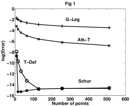
Fig. 1: Comparison of numerical solutions of Example 1,   $\lambda=0.1$.   

Example 2.

$$x(t)+{\lambda}\int^{T}_{0}k(t,s)x(s)ds=y(t),\ \ \ 0\leq t\leq T$$

where $y(t)=(1-\frac{{\lambda}sin^{2}(T)}{2}+{\lambda})sint+(\frac{T}{2}-t-\frac{sin(2T)}{4}){\lambda}cost,$  and

$$k(t,s)=sin(|t-s|)\\ =\left\{\begin{array}[]{cc}sin(t-s)&{\rm if}\ \ 0\leq s\leq t\\ sin(s-t)&{\rm if}\ \ t<s\leq\frac{\pi}{2}.\end{array}\right.$$

The analytical solution is $x(t)=sin(t)$. This kernel has discontinuities in the first order partial derivatives along the diagonal, $t=s.$ Again standard $Nystr{\ddot{o}}m$-type discretization methods fail to give high accuracy in this case. In the first experiment we take $T=\frac{\pi}{2}$  and $\lambda=-\frac{4}{\pi}.$ Our method shows the order of $10^{-14}$ accuracy with only 16 points in $[0,\frac{\pi}{2}]$ without any partitioning. The 2-step method of Deferred Approach to the Limit gives the accuracy of ${\it{O}}(10^{-14})$ with $n=256,$ but at much higher cost than our method, see Fig 2. The second part of Example 2 is to compare the composite rule described in Section 5 with the basic quadrature (53) of Section 4 when the length of the interval of integration, $[a,b]$, becomes increasingly large. Here $M$ denotes the number of subintervals in $[0,T]$ and $Mn$ stands for the total number of support points in the given interval $[0,T].$

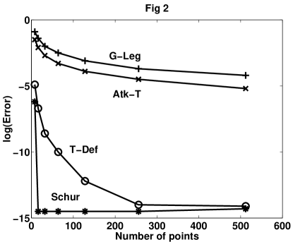
Fig. 2: Comparison of numerical solutions of Example 2.

Table 1 (  $T=200\pi,$   $\lambda=-\frac{4}{\pi}$  )

$M$	1	1	1	2	4	8
$Mn$	$256$	$512$	$1024$	$256$	$512$	$1024$
Error	$2.4e+01$	$3.0e-02$	CPUtime limit exceed	$1.2e+01$	$7.8e-02$	$2.2e-11$

Without partitioning, i.e. with $M=1$, we increase the number of support points from $n=128$ to $n=1024.$  For $n=512$ the accuracy is of order ${\it{O}}(10^{-2}),$  but for $n=1024$   the CPU time limit is exceeded. When the interval is partitioned into $8$ subintervals and $n=128$ i.e., the total number of points is $1024,$ the accuracy now is of order ${\it{O}}(10^{-11}).$
Example 3.

$$x(t)+\int^{1}_{-1}k(t,s)x(s)ds=y(t),\ \ \ -1\leq t\leq 1$$

where $y(t)=1-t^{2}+\frac{1}{1-t^{2}}(\arctan(t)-\arctan(-1))-\frac{1}{(1+t)(1+t^{2})},$ and

$$k(t,s)=\left\{\begin{array}[]{cc}\frac{1}{(1-t^{2})(1-s^{4})}&{\rm if}\ \ -1\leq s\leq t\\ \frac{-1}{(1-t^{4})(1-s^{2})}&{\rm if}\ \ \ \ t<s\leq 1.\end{array}\right.$$

The analytical solution is $x(t)=1-t^{2}$. Since this kernel has singularities along the boundaries of the square $[-1,1]\times[-1,1]$ methods based on the Trapezium rule are not applicable. Therefore we compare our algorithms of Section 1 and Section 3 with the $Nystr{\ddot{o}}m$-Gauss-Legendre discretization only. The algorithm of Section 1 shows the same accuracy of numerical solution as the Gauss-Legendre quadrature. The method of Section 3 gives ${\it{O}}(10^{-13})$ accuracy with $n=32$ points, whereas $Nystr{\ddot{o}}m$-Gauss-Legendre quadrature gives ${\it{O}}(10^{-3})$ with $n=256$ points.

Fig. 3: Comparison of numerical solutions of Example 3.

Example 4.

$$x(t)+\int^{1}_{-1}k(t,s)x(s)ds=y(t),\ \ \ -1\leq t\leq 1$$

where $y(t)=2(1-t^{2}+2t^{3})+(1+2t^{4})ln(t^{2}+t^{4})-ln(1+t^{2})-2t^{4}ln(1+t^{4}),$  and

$$k(t,s)=\left\{\begin{array}[]{cc}1/(t^{2}+s^{4})&{\rm if}\ \ -1\leq s\leq t\\ 1/(s^{2}+t^{4})&{\rm if}\ \ t<s\leq 1.\end{array}\right.$$

The analytical solution is $x(t)=4t^{3}$. The kernel $k(t,s)$ has a singularity at $(0,0)$. Also $y(t)$ is singular at $t=0$. Since Chebyshev points $cos(\frac{(2i-1)}{2N}\pi)$,  $i=1,2,...,n,$ are clustered towards the end points of interval $[-1,1],$ discretization formula (53) does not contain sufficient values of kernel near $(t,s)=(0,0)$. Therefore we partition $[-1,1]$ into $[-1,0]$ and $[0,1].$ The choice of $n=256$ Chebyshev points in each subinterval with the total of $n=512$ points gives ${\it O}(10^{-11})$ accuracy. For comparison the best accuracy of the Gauss-Legendre quadrature without partitions and with $n=512$ support points is ${\it{O}}(10^{-4})$ while the best accuracy of the algorithm of Section 2 without partitions is of ${\it O}(10^{-6}),$ see Fig 4.

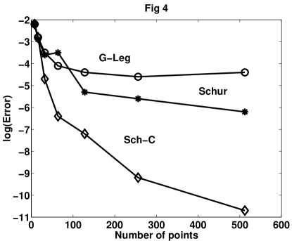
Fig. 4: Comparison of numerical solutions of Example 4.

7 Application to Non-Local Schroedinger Equations

In this section we demonstrate that the developed numerical technique is also applicable to problems other than integral equations, for example, to integro-differential equations. We chose here the radial Schroedinger equation which models the quantum mechanical interaction between particles represented by spherically symmetric potentials. These potentials are usually local, i.e., they depend only on the distance between the two particles, in which case the equation is a differential equation which is routinely solved in computational physics. However, if there are more than two particles present, then the potentials can become non-local and the differential Schroedinger equation becomes an integro-differential equation for the wave function $\psi,$

$$\frac{d^{2}\psi(r)}{dr^{2}}+{\kappa}^{2}\psi(r)=\int^{T}_{0}v(r,r^{\prime})\psi(r^{\prime})dr^{\prime},$$ (101)

which is defined for $0<r<\infty$, satisfies the condition $\psi(0)=0,$ and is bounded at infinity. It is assumed that $v(r,r^{\prime})$ is negligible for $r>T$ or $r^{\prime}>T,$ see e.g. [13]. Because it is numerically more difficult to solve the Schroedinger equation in the presence of a nonlocal potential, the latter is customarily replaced by an approximate local equivalent potential. There is, however, a renewed interest in the nonlocal equations, and a significant number of papers on this subject appeared in the past few years, (our database search returned over 50 related publications).

Using the technique of [8] it easy to show that (101) is equivalent to the following integral equation,

$$\psi(r) + \frac{cos(\kappa r)}{\kappa}\int^{r}_{0}sin(\kappa r^{\prime})\int^{T}_{0}v(r^{\prime},p)\psi(p)dpdr^{\prime}$$

$$+ \frac{sin(\kappa r)}{\kappa}\int^{T}_{r}cos(\kappa r^{\prime})\int^{T}_{0}v(r^{\prime},p)\psi(p)dpdr^{\prime}=sin({\kappa}r).$$

or

$$\psi(r)+\frac{cos(\kappa r)}{\kappa}\int^{T}_{0}k_{1}(r,r^{\prime})\psi(r^{\prime})dr^{\prime}+\frac{sin(\kappa r)}{\kappa}\int^{T}_{0}k_{2}(r,r^{\prime})\psi(r^{\prime})dr^{\prime}$$ (102)

$$=sin(\kappa r),$$

where

$$k_{1}(r,r^{\prime})=\int^{r}_{0}sin(\kappa p)v(p,r^{\prime})dp,\ \ \ k_{2}(r,r^{\prime})=\int^{T}_{r}cos(\kappa p)v(p,r^{\prime})dp.$$

We consider now the case when $v(p,r^{\prime})$ is $(p_{1},p_{2})$-semismooth, such that

$$v(p,r^{\prime})=\left\{\begin{array}[]{cc}v_{1}(p,r^{\prime})&{\rm if}\ \ 0\leq p\leq r^{\prime}\\ v_{2}(p,r^{\prime})&{\rm if}\ \ r^{\prime}\leq p\leq T.\end{array}\right.$$

In order to use the method which we developed in previous sections, we rewrite equation (102) as follows,

$$\psi(r)+\frac{c(r)}{\kappa}\int^{r}_{0}k_{1}(r,r^{\prime})\psi(r^{\prime})dr^{\prime}+\frac{c(r)}{\kappa}\int^{T}_{r}k_{1}(r,r^{\prime})\psi(r^{\prime})dr^{\prime}$$

$$+\frac{s(r)}{\kappa}\int^{r}_{0}k_{2}(r,r^{\prime})\psi(r^{\prime})dr^{\prime}+\frac{s(r)}{\kappa}\int^{T}_{r}k_{2}(r,r^{\prime})\psi(r^{\prime})dr^{\prime}=s(r),$$ (103)

where for notational convenience we abbreviate,  $c(r)=cos(\kappa r),s(r)=sin(\kappa r).$ We have

$$k_{1}(r,r^{\prime})=\left\{\begin{array}[]{cc}k_{11}(r,r^{\prime})&{\rm if}\ \ 0\leq r^{\prime}\leq r\\ k_{12}(r,r^{\prime})&{\rm if}\ \ 0\leq r\leq r^{\prime},\end{array}\right.$$

and

$$k_{2}(r,r^{\prime})=\left\{\begin{array}[]{cc}k_{21}(r,r^{\prime})&{\rm if}\ \ r^{\prime}\leq r\leq T\\ k_{22}(r,r^{\prime})&{\rm if}\ \ r\leq r^{\prime}\leq T,\end{array}\right.$$

where

$$k_{11}(r,r^{\prime}) = \int^{r^{\prime}}_{0}s(p)v_{1}(p,r^{\prime})dp+\int^{r}_{r^{\prime}}s(p)v_{2}(p,r^{\prime})dp,$$

$$= \int^{r^{\prime}}_{0}s(p)v_{1}(p,r^{\prime})dp+\int^{r}_{0}s(p)v_{2}(p,r^{\prime})dp-\int^{r^{\prime}}_{0}s(p)v_{2}(p,r^{\prime})dp,$$

$$k_{12}(r,r^{\prime}) = \int^{r}_{0}s(p)v_{1}(p,r^{\prime})dp$$

$$k_{21}(r,r^{\prime}) = \int^{T}_{r}c(p)v_{2}(p,r^{\prime})dp$$

$$k_{22}(r,r^{\prime}) = \int^{r^{\prime}}_{r}c(p)v_{1}(p,r^{\prime})dp+\int^{T}_{r^{\prime}}c(p)v_{2}(p,r^{\prime})dp,$$

$$= \int^{T}_{r}c(p)v_{1}(p,r^{\prime})dp-\int^{T}_{r^{\prime}}c(p)v_{1}(p,r^{\prime})dp+\int^{T}_{r^{\prime}}c(p)v_{2}(p,r^{\prime})dp.$$

Thus,

$$\psi(r)+\frac{c(r)}{\kappa}\int^{r}_{0}k_{11}(r,r^{\prime})\psi(r^{\prime})dr^{\prime}+\frac{c(r)}{\kappa}\int^{T}_{r}k_{12}(r,r^{\prime})\psi(r^{\prime})dr^{\prime}$$

$$+\frac{s(r)}{\kappa}\int^{r}_{0}k_{21}(r,r^{\prime})\psi(r^{\prime})dr^{\prime}+\frac{s(r)}{\kappa}\int^{T}_{r}k_{22}(r,r^{\prime})\psi(r^{\prime})dr^{\prime}=s(r),$$ (104)

Applying our quadrature to this equation we get,

$$[\ {\bf{I}}+\frac{T}{2\kappa}{\bf{D}}_{c}({\bf{W}}\circ{\bf{K}}_{11}+{\bf{V}}\circ{\bf{K}}_{12})+\frac{T}{2\kappa}{\bf{D}}_{s}({\bf{W}}\circ{\bf{K}}_{21}+{\bf{V}}\circ{\bf{K}}_{22})\ ]{\bar{\bf{\psi}}}={\bar{\bf{s}}},$$ (105)

where in more detail,

$${\bar{\bf{\psi}}} = [\psi(t_{0}),\psi(t_{1}),...,\psi(t_{n})]^{T},$$

$${\bf{D}}_{c} = diag(cos(\kappa t_{0}),cos(\kappa t_{1}),...,cos(\kappa t_{n})),$$

$${\bf{D}}_{s} = diag(sin(\kappa t_{0}),sin(\kappa t_{1}),...,sin(\kappa t_{n})),$$

$${\bf{D}}_{\sigma} = diag([1,...,1]{\bf{S}}_{L}{\bf{C}}^{-1}),$$

$${\bar{\bf{s}}} = [sin(\kappa t_{0}),sin(\kappa t_{1}),...,sin(\kappa t_{n})]^{T},$$

$${\bf{W}} = {\bf{C}}{\bf{S}}_{L}{\bf{C}}^{-1},\ \ \ {\bf{V}}={\bf{C}}{\bf{S}}_{R}{\bf{C}}^{-1},$$

$${\bf{K}}_{11} = (k_{11}(t_{i},t_{j}))^{n}_{i,j=0}$$

$$= \frac{T}{2}[diag({\bf{W}}{\bf{D}}_{s}({\bf{V}}_{1}-{\bf{V}}_{2}))+({\bf{W}}{\bf{D}}_{s}{\bf{V}}_{2})]$$

$${\bf{K}}_{12} = (k_{12}(t_{i},t_{j}))^{n}_{i,j=0}$$

$$= \frac{T}{2}({\bf{W}}{\bf{D}}_{s}{\bf{V}}_{1}),$$

$${\bf{K}}_{21} = (k_{21}(t_{i},t_{j}))^{n}_{i,j=0},$$

$$= \frac{T}{2}({\bf{V}}{\bf{D}}_{c}{\bf{V}}_{2})$$

$${\bf{K}}_{22} = (k_{22}(t_{i},t_{j}))^{n}_{i,j=0}$$

$$= \frac{T}{2}[({\bf{V}}{\bf{D}}_{c}{\bf{V}}_{1})+diag({\bf{V}}{\bf{D}}_{c}({\bf{V}}_{2}-{\bf{V}}_{1}))].$$

We illustrate now the obtained discretization with two examples. In the first example we use a prototype of the Yukawa potential, (e.g. [12], 23.c), which is simplified to a degree such that an analytic solution can be found. In our terminology this potential is semiseparable. We note once more that the case of this semi-separable potential could be treated more easily by the techniques already presented in [8], and we use it here only because the comparison with the analytic solution is possible.
Example 1. Let

$$v(p,r^{\prime})=\left\{\begin{array}[]{cc}\lambda e^{p-r^{\prime}}&{\rm if}\ \ 0\leq p\leq r^{\prime}\\ \lambda e^{r^{\prime}-p}&{\rm if}\ \ r^{\prime}\leq p\leq T.\end{array}\right.$$

It is easy to see that if $\psi(r)=e^{-r},$ then the right-hand side has the form,

$$y(r)=(1-\frac{3{\lambda}{\kappa}}{4})e^{-r}+\frac{3{\lambda}{\kappa}}{4}cos(r)-\frac{{\lambda}{\kappa}}{2}re^{-r}.$$

By comparing the analytical solution given above with the numerical solution of (105) at the discretization points, we get the following relative errors in the case of ${\lambda}=0.1,\ \ {\kappa}=1$   and  $T=20.$

$n$	16	32	64	128	256
$Error$	$1.2e+01$	$3.4e-07$	$8.1e-09$	$3.4e-09$	$6.0e-09$

In the second example we consider a more interesting case for which the techniques of [8] are not applicable. This time the non-locality is a prototype of the optical model Perey-Buck potential, (e.g. [6], Ch. V.2). In our terminology this potential is semi-smooth, but not semiseparable.
Example 2. Let

$$v(p,r^{\prime})=\frac{{\lambda}e^{-\frac{|r^{\prime}-p|}{A}}}{1+e^{-\frac{|r^{\prime}-p|}{A}}}=\left\{\begin{array}[]{cc}\frac{\lambda e^{\frac{p-r^{\prime}}{A}}}{1+e^{\frac{p-r^{\prime}}{A}}}&{\rm if}\ \ 0\leq p\leq r^{\prime}\\ \frac{\lambda e^{\frac{r^{\prime}-p}{A}}}{1+e^{\frac{r^{\prime}-p}{A}}}&{\rm if}\ \ r^{\prime}\leq p\leq T.\end{array}\right.$$

Solving (105) at $n$ shifted Chebyshev support points $t^{(n)}_{i},i=1,...,n,$ and $2n$ points $s^{(2n)}_{i},i=1,...,2n,$ we obtain numerical solutions ${\psi}^{(n)}(r)$ and ${\psi}^{(2n)}(r)$, respectively.

To get the values of ${\psi}^{(2n)}(r)$ at $t^{(n)}_{i},$ we follow the procedure described in the beginning of Section 6. The error $e_{n}$ is obtained by comparison of the solutions ${\psi}^{(n)}$  and ${\psi}^{(2n)}$  as follows,

$$e_{n}=||{\psi}^{(2n)}(t^{(n)}_{i})-{\psi}^{(n)}(t^{(n)}_{i})||_{\infty}/||{\psi}^{(2n)}(t^{(n)}_{i})||_{\infty}.$$

Here we take $\lambda=0.1$, $\kappa=1,$  $A=100,$  and  $T=20.$

$n$	8	16	32	64	128	256
$e_{n}$	$1.0e-0$	$1.2e-03$	$1.6e-09$	$7.7e-15$	$1.6e-14$	$4.8e-14$

We see that for this choice of $\lambda$ the matrix is well conditioned and the double precision accuracy is obtained with 64 points.

8 Summary and Conclusions

In this paper, which is one of a sequence treating integral equations, we describe a new method for solving integral equations for the case when kernel can be discontinuous along the main diagonal. It has the following advantages for a large class of such kernels: (i) for semismooth kernels it gives a much higher accuracy than it was ever possible with standard Gauss type quadrature rules; (ii) it is of comparable accuracy with Gauss type quadratures for smooth kernels; (iii) it exploits additional structure of the kernel such as a low semi-rank, or a displacement structure, for example, to allow for reduced complexity algorithms for the discretized equations. (iv) the numerical examples provided in the present study illustrate increased accuracy of our method compared to other more conventional methods.

Our method is also applicable to other problems, such as the computation of eigenvalues and eigenfunctions of integral and differential operators and solution of integro-differential equations.

Our method may find applications in quantum mechanical atomic and nuclear physics problems, where the requirement of indistinguishability of the electrons leads to non localities in the potential contained in the Schroedinger equation due to the presence of exchange terms. These, in turn, lead to integro-differential equations which are usually solved by iterative finite difference methods, or by orthogonal function expansion methods. We plan to compare our new method with some of the existing methods in future investigations on more realistic examples.

References

• [1] P.M. Anselone, Collectively Compact Operator Approximation Theory and Applications to Integral Equations, Prentice-Hall, Englewood Hills, 1971.
• [2] K.E. Atkinson, A Survey of Numerical Methods for the Solution of Fredholm Integral Equations of the Second Kind, SIAM, Philadelphia, 1976.
• [3] C.T.H. Baker, The Numerical Treatment of Integral Equations, Oxford University Press, 1977.
• [4] C.W. Clenshaw and A. R. Curtis, A method for numerical integration on an automatic computer, Numer. Math. 2, 197(1960).
• [5] L.M. Delves and J.L. Mohamed, Computational Methods for Integral Equations, Cambridge University Press, Cambridge, 1985.
• [6] H. Feshbach, Theoretical Nuclear Physics, Nuclear Physics, John Wiley and Sons, 1992.
• [7] I. Gohberg and I.A. Fel’dman, Convolution Equations and Projection Methods for Their Solution, Transl. Math. Monograph, Vol 41, American Mathematical Society, Providence, RI, 1974.
• [8] R.A Gonzales, J. Eisert, I. Koltracht, M. Neumann and G. Rawitscher, Integral Equation Method for the Continuous Spectrum Radial Schroedinger Equation, J. of Comput. Phys. 134, 134-149, 1997.
• [9] R.A Gonzales, S.-Y. Kang, I. Koltracht and G. Rawitscher, Integral Equation Method for Coupled Schroedinger Equations, J. of Comput. Phys. 153, 160(1999).
• [10] D. Gottlieb and S. Orszag, Numerical Analysis of Spectral Methods, SIAM, Philadelphia, 1977.
• [11] L. Greengard and V. Rokhlin, On the Numerical Solution of Two-Point Boundary Value Problems, Commun. Pure Appl. Math. 44, 419(1991).
• [12] R.H. Landau, Quantum Mechanics II, John Wiley and Sons, 1990.
• [13] N.F. Mott and H.S. Massey, The Theory of Atomic Collision, 3rd ed. Oxford, Clarendon 1965.
• [14] G.H. Rawitscher, B.D. Esry, E. Tiesinga, P. Burke, Jr. and I. Koltracht Comparison of Numerical Methods for the Calculation of Cold Atomic Collisions, Submitted to J. Chem. Phys.
• [15] L. Reichel, Fast Solution Methods for Fredholm Integral Equations of the Second Kind, Numer. Math. 57, 719(1989).
• [16] H.L. Royden, Real Analysis, 3-rd Edition, Macmillan Publishing Company, NY, 1989.