More Monotone Open Homogeneous Locally Connected Plane Continua

Abstract.

This paper constructs a continuous decomposition of the Sierpiński curve into acyclic continua one of which is an arc. This decomposition is then used to construct another continuous decomposition of the Sierpiński curve. The resulting decomposition space is homeomorphic to the continuum obtained from taking the Sierpiński curve and identifying two points on the boundary of one of its complementary domains. This outcome is shown to imply that there are continuum many topologically different one dimensional locally connected plane continua that are homogeneous with respect to monotone open maps.

1. Introduction

In a recent paper [P1998], J. R. Prajs remarks without proof that there are infinitely many topologically different locally connected plane continua that are homogeneous with respect to monotone open mappings. These spaces are described as two dimensional and monotone open equivalent to the Sierpiński curve. Here, using the construction techniques developed in [S1998] to prove that the Sierpiński curve is monotone open homogeneous, we prove that there are continuum many one dimensional locally connected plane continua that are monotone open homogeneous. A continuum, $X$, is monotone open homogeneous if for any two points, $x$ and $y$, in $X$ there is a monotone open map from $X$ onto $X$ so that $f(x)=y$. A monotone map is one with connected fibers and an open map is one that preserves open sets. By map we mean a continuous function. We say two continua, $X$ and $Y$, are monotone open equivalent if there is a monotone open map from $X$ onto $Y$ and vice versa.

This paper makes use of the fact that there is a continuous decomposition of the Sierpiński curve into acyclic continua, one of which is an arc lying in the boundary of the unbounded complementary domain, such that the decomposition space is homeomorphic to the Sierpiński curve. The details of the construction of such a decomposition are given in Section 3–5 of this paper and are almost identical to the continuous decomposition described in [S1998]; the only difference being that there in the final stage of the construction the decomposition elements are wrapped around a bounded complementary domain, while here the decomposition elements are stretched and bent in order to lie alongside an arc on the boundary of the unbounded complementary domain. This decomposition can be used to show that there is a continuous decomposition of the Sierpiński curve into acyclic continua so that the decomposition space is homeomorphic to the continuum which results from taking the Sierpiński curve and identifying two points on the boundary of a bounded complementary domain. Combining this result with those of [S1998], we get that this last continuum is monotone open equivalent to the Sierpiński curve and so is also monotone open homogeneous. A generalization of this result shows that there are continuum many locally connected plane continua that are monotone open homogeneous. This result, however, leaves open the question asked by J. Prajs on whether or not there might exist a nondegenerate locally connected plane continuum that is monotone open homogeneous but is not either a simple closed curve or monotone open equivalent to the Sierpiński curve.

2. Main Result

In this section we will assume the following theorem, which will be proved in the remaining sections of the paper. The proof of the theorem in Sections 3–5 in no way depends on the results in Section 2.

Theorem 2.1.

There exists a continuous decomposition of the Sierpiński curve into acyclic continua, one of which is an arc lying in the boundary of the unbounded complementary domain, such that the decomposition space is homeomorphic to the Sierpiński curve.

We will call a bounded complementary domain of the Sierpiński curve a hole. We will call the continuum that results from taking a Sierpiński curve and identifying $n$ points on the boundary of one hole of the curve a Sierpiński curve with one pinched hole with $n$ lobes. Notice that a Sierpiński curve with one pinched hole has one local cut point, which we will call the center of the pinched hole. Given a Sierpiński curve with one pinched hole we call the union of the complementary domains which have boundaries that intersect at the local cut point a pinched hole, while each such complementary domain is called a lobe of the pinched hole. We remark that using the same techniques that are used in [W1958] by G. T. Whyburn to prove that two $S$-curves are homeomorphic, we can prove that if we have two Sierpiński curves each with one pinched hole with $n$ lobes, then they are homeomorphic. We will also need the notion of a pinched hole with a pinched lobe. By a Sierpiński curve with one pinched hole with $n$ lobes one of which is pinched we mean the continuum that results from identifying two points of the boundary of a lobe of a pinched hole where neither of the points are the center of the pinched hole.

By the standard square Sierpiński curve, we mean the Sierpiński curve that results from removing open square holes from the unit square $[0,1]\times[0,1]$ in the standard way. Specifically, let $S_{1}=I\times I$ and $S_{2}$ be the continuum that results from dividing $S_{1}$ into $9$ identical squares and removing the interior of the center one. For $i\in\operatorname{\mathbb{Z}}^{+}$, we obtain $S_{i+1}$ by taking each of the $8^{(i-1)}$ squares that make up $S_{i}$ and dividing it into $9$ identical squares and then removing the interior of the center one. The standard square Sierpiński curve is $S=\cap^{\infty}_{i=1}S_{i}$.

Using Theorem 2.1 we are able to prove the following theorem:

Theorem 2.2.

Let $B$ be a Sierpiński curve with one pinched hole with two lobes. Then there is a continuous decomposition of the Sierpiński curve into acyclic continua so that the decomposition space is homeomorphic to $B$.

Proof.

Let $S$ be the standard square Sierpiński curve. From Theorem 2.1 there is a continuous decomposition $G_{1}$ of $S$ into acyclic continua one of which is an arc that without loss of generality we can assume is the left edge of $S$. We can also assume that $S/G_{1}$ is the Sierpiński curve $T(S)$ where $T:S\rightarrow{\operatorname{\mathbb{E}}}^{2}:(x,y)\mapsto(x,yx)$. In addition we would like to assume that the members of $G_{1}$ that lie along the right edge of $S$ are single points. To see that we can make this assumption without loss of generality consider the following argument. Let ${g:S\rightarrow S/G_{1}}$ be the natural map and consider the decomposition space $Z$ that results from collapsing to points all the members of $G_{1}$ that intersect the right edge of $S$. We will denote by $\phi$ this quotient map. Since the right edge of $S$ is a closed set and $g$ is a closed map it can be shown that $\phi$ is closed. Also since $g$, in addition to being closed, is monotone and open, the map $\pi^{\prime}:Z\rightarrow S/G_{1}$ defined by $\pi^{\prime}(z)=f(\phi^{-1}(z))$ is closed, monotone, and open. Finally, since $\phi$ is a homeomorphism on the boundary points of the complementary domains of $S$ it can be shown using results of [W1958] that $Z$ is homeomorphic to the Sierpiński curve. Now $\pi^{\prime}$ induces a continuous decomposition of $Z$ into acyclic continua so that in addition to one element of the decomposition lying along the boundary of the unbounded complementary domain there is another arc of the unbounded complementary domain that is the union of degenerate elements of the decomposition. Thus we can assume without loss of generality that the members of $G_{1}$ that lie along the right edge of $S$ are single points. Let $\pi_{1}$ be the quotient map from $S$ to $S/G_{1}$.

Let $G_{2}$ be a continuous decomposition of $S$ into acyclic continua with the quotient map $\pi_{2}$ so that $S/G_{2}=T^{\prime}(S)$ where $T^{\prime}:S\rightarrow{\operatorname{\mathbb{E}}}^{2}:{(x,y)\mapsto(x,y(1-x))}$; so that $\pi_{2}^{-1}((1,0))$ is the right edge of $S$; and so that $\pi_{2}$ is the identity on the left side of $S$. See Figure 1.

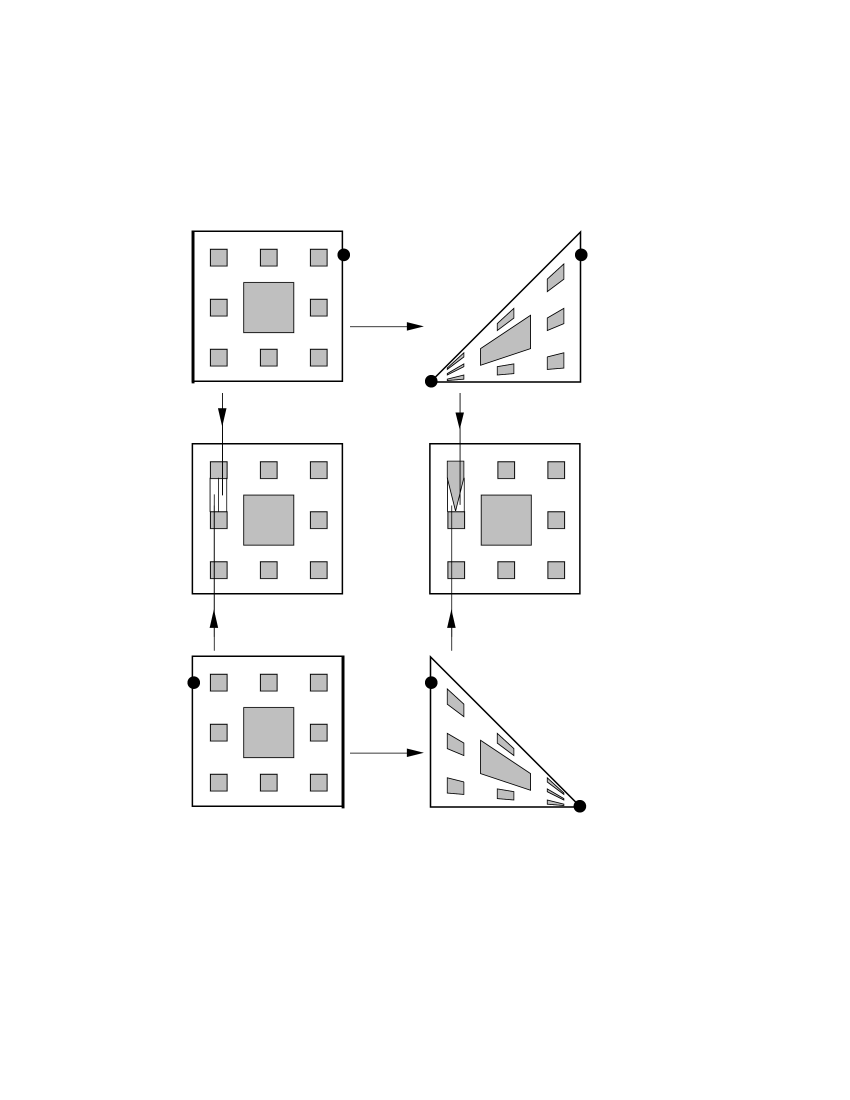
Figure 1. There is a monotone open map from $S$ to $B$.

Let $h_{1}:S\rightarrow([\frac{1}{6},\frac{2}{9}]\times[\frac{5}{9},\frac{7}{9}]):(x,y)\mapsto(\frac{1}{18}x+\frac{1}{6},\frac{2}{9}y+\frac{5}{9})$ and $h_{2}:S\rightarrow([\frac{1}{9},\frac{1}{6}]\times[\frac{5}{9},\frac{7}{9}]):(x,y)\mapsto(\frac{1}{18}x+\frac{1}{9},\frac{2}{9}y+\frac{5}{9})$. Denote by $S^{\prime}$ the Sierpiński curve that results from removing the rectangles $([\frac{1}{9},\frac{1}{6}]\times[\frac{5}{9},\frac{7}{9}])$ and $([\frac{1}{6},\frac{2}{9}]\times[\frac{5}{9},\frac{7}{9}])$ from $S$ and replacing them with $h_{2}(S)$ and $h_{1}(S)$ respectively. Denote by $B$ the Sierpiński curve with one pinched hole with two lobes that results from removing the rectangles $([\frac{1}{9},\frac{1}{6}]\times[\frac{5}{9},\frac{7}{9}])$ and $([\frac{1}{6},\frac{2}{9}]\times[\frac{5}{9},\frac{7}{9}])$ from $S$ and replacing them with $h_{2}(S/G_{2})$ and $h_{1}(S/G_{1})$ respectively. We can now define the map $f:{\operatorname{\mathbb{E}}}^{2}\rightarrow{\operatorname{\mathbb{E}}}^{2}$ as follows:

$$f(x,y)=\left\{\begin{array}[]{ll}h_{1}\circ\pi_{1}\circ h_{1}^{-1}(x,y)&\mbox{if $(x,y)\in([\frac{1}{6},\frac{2}{9}]\times[\frac{5}{9},\frac{7}{9}])$;}\\ h_{2}\circ\pi_{2}\circ h_{2}^{-1}(x,y)&\mbox{if $(x,y)\in([\frac{1}{9},\frac{1}{6}]\times[\frac{5}{9},\frac{7}{9}])$;}\\ (x,y)&\mbox{otherwise.}\end{array}\right.$$

Thus $f|S^{\prime}$ is a continuous function from $S^{\prime}$ onto $B$ which is monotone and open because $\pi_{1}$ and $\pi_{2}$ are monotone open maps. Therefore the theorem holds. ∎

Corollary 2.3.

Let $B$ be a Sierpiński curve with one pinched hole with $n$ lobes with $n\in\operatorname{\mathbb{Z}}^{+}$. Then there is a continuous decomposition of the Sierpiński curve into acyclic continua so that the decomposition space is homeomorphic to $B$.

The proof this corollary is very similar in style to the proof of Theorem 2.2; however, here we must repeat the construction described $n-1$ more times. In each of these constructions we collapse an arc that has one end point at the center of a pinched hole and another end point on the boundary of a different hole and avoids all other boundary points of holes.

Corollary 2.4.

Let $B$ be a Sierpiński curve with one pinched hole with $n$ lobes one of which is pinched where $n\in\operatorname{\mathbb{Z}}^{+}$. Then there is a continuous decomposition of the Sierpiński curve into acyclic continua so that the decomposition space is homeomorphic to $B$.

To prove this corollary we can use the techniques used in the proof of Theorem 2.2 to collapse an arc that has one end point on the boundary of a lobe (other than the center point of a pinched hole) and the other end point on the boundary of another hole and avoids all other boundary points of holes.

Theorem 2.5.

If $B$ is a Sierpiński curve with a pinched hole with two lobes, then there is a monotone open map from $B$ onto a Sierpiński curve.

Proof.

From the construction described in [S1998] we know that there is a monotone open map, $g$, from the Sierpiński curve, $S$, onto $S$ so that for some $p\in S$, $g^{-1}(p)$ is the boundary of a hole. Consider the identification $\phi$ of two points of $g^{-1}(p)$. Now $\phi$ is a closed map and it can be shown using techniques used in [W1958] that the image of $S$ under $\phi$ is homeomorphic to $B$. Let $h$ be homeomorphism from $B$ onto $\phi(S)$. Since $g$ is open and closed the map $g\circ\phi^{-1}\circ h$ is a monotone open map from $B$ to $S$. ∎

We now have the following two corollaries which can be proved as above.

Corollary 2.6.

If $B$ is a Sierpiński curve with a pinched hole with $n$ lobes, then there is a monotone open map from $B$ onto a Sierpiński curve.

Corollary 2.7.

If $B$ is a Sierpiński curve with a pinched hole with $n$ lobes one of which is pinched, then there is a monotone open map from $B$ onto a Sierpiński curve.

Now consider a Sierpiński curve with a sequence of pinched holes. Specifically, let $B_{0}$ be the standard square Sierpiński curve and for each $n\in\operatorname{\mathbb{Z}}^{+}$ let $B_{n}$ be a Sierpiński curve with one pinched hole with $n+1$ lobes so that the boundary of the unbounded component of the complement is the same as the boundary of the rectangle

$$\Bigl{[}\sum^{n-1}_{i=0}\Bigl{(}\frac{1}{3}\Bigr{)}^{i},\sum^{n}_{i=0}\Bigl{(}\frac{1}{3}\Bigr{)}^{i}\Bigr{]}\times\Bigl{[}0,\Bigl{(}\frac{1}{3}\Bigr{)}^{n}\Bigr{]}.$$

See Figure 2.

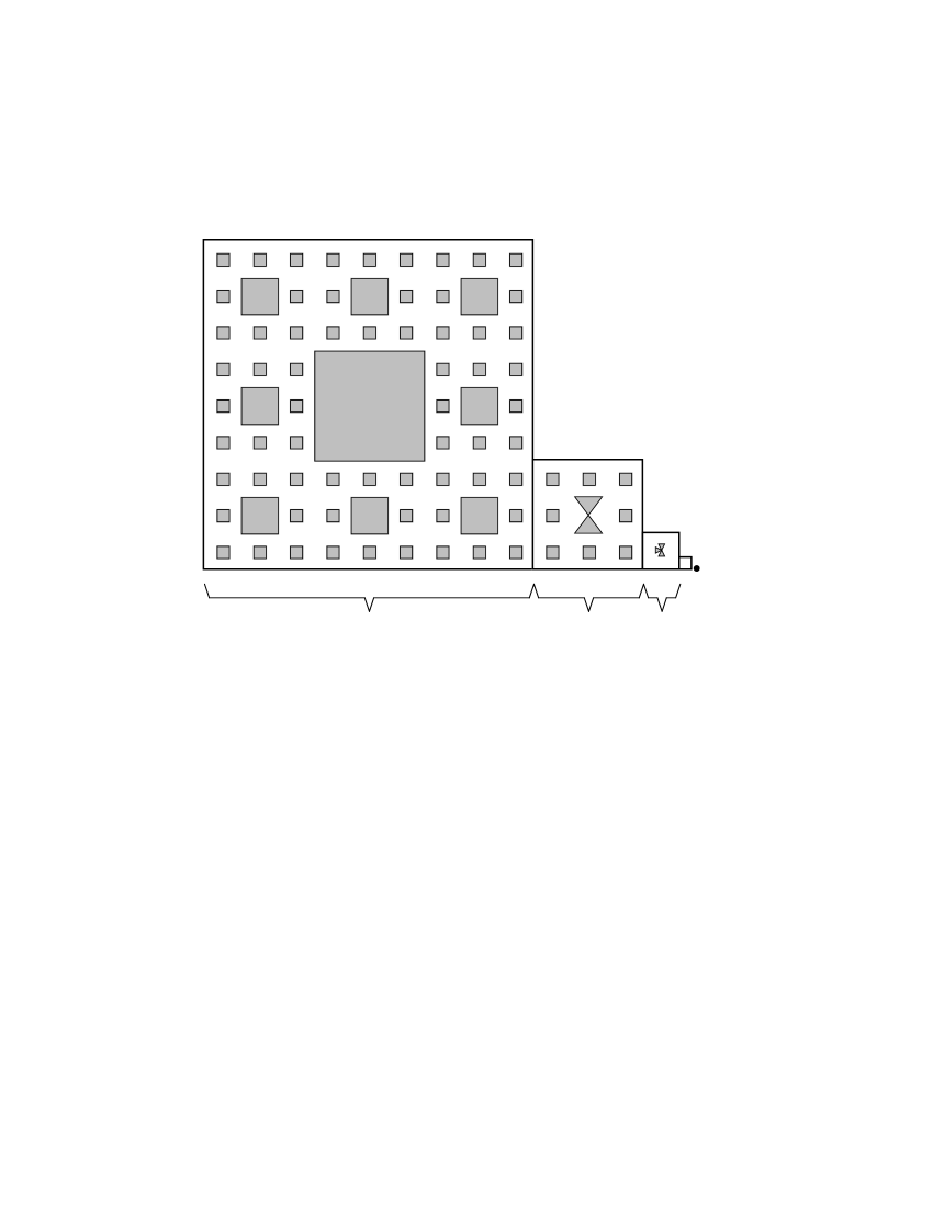
Figure 2. Figures like $B=\cup_{i=0}^{\infty}B_{i}\cup\{(\frac{3}{2},0)\}$ are monotone open homogeneous.

Let $B$ be the closure of $\cup B_{n}$. We will now show that $B$ is monotone open homogeneous. Let $S_{0}$ be the standard Sierpiński curve and $S_{n}$ be a Sierpiński curve with the same unbounded complementary domain as $B_{n}$. Let $S$ be the closure of $\cup S_{n}$. By Whyburn’s characterization of the Sierpiński curve [W1958] we know that $S$ is a Sierpiński curve. From Corollary 2.3 there is a monotone open map $f_{n}$ from $S_{n}$ onto $B_{n}$ for each non-negative integer. In fact there exists such a map $f_{n}$ that is the identity on the boundary of the unbounded complementary domain of $S_{n}$. Define $f:S\rightarrow B$ as follows:

$$f(x)=\left\{\begin{array}[]{ll}f_{n}(x)&\mbox{if $x\in S_{n}$;}\\ x&\mbox{otherwise.}\end{array}\right.$$

Now $f$ is continuous, monotone, and open. From Corollary 2.6 we can similarly construct a monotone open map $g$ from $B$ onto $S$. Thus $B$ is monotone open equivalent to $S$. Since $S$ is monotone open homogeneous [S1998] we have that $B$ is monotone open homogeneous.

Now consider $r\in[0,1]$ and let $0.b_{1}b_{2}b_{3}...$ be the binary representation of $r$. We can create a new continuum $B^{r}$ by either pinching or not pinching one of the lobes of the pinched hole of $B_{n}$ depending on whether or not $b_{n}$ is $0$ or $1$. For each $r\in[0,1]$ using corollaries 2.3, 2.4, 2.6, and 2.7 we can show that $B^{r}$ is monotone open equivalent to $S$ and so is monotone open homogeneous. Since $B^{r}$ is not homeomorphic to $B^{r^{\prime}}$ unless $r=r^{\prime}$, we have proved the following theorem.

Theorem 2.8.

There are continuum many topologically different locally connected plane continua that are monotone open homogeneous.

The remainder of the paper describes a construction that proves Theorem 2.1. This construction follows that described in [S1998] very closely and in fact, much is identical but is included here to simplify the reading of this paper. Note that J. Prajs has suggested [P1999] an alternate proof to Theorem 2.1 based on the fact that there is a continuous decomposition of the Sierpiński curve into pseudo-arcs and on a lemma about extending functions on Sierpiński curves.

3. Preliminaries and Overview of Construction

Before giving an overview of our construction we introduce the following notation. If $P$ is a collection of sets, then $P^{*}$ denotes the union of members of $P$. If $p$ is a set, then $\operatorname{st}^{1}(p,P)=\{p^{\prime}\in P:p^{\prime}\cap p\neq\emptyset\}$ and inductively $\operatorname{st}^{i+1}(p,P)=\operatorname{st}^{1}(\operatorname{st}^{i}(p,P)^{*},P)$. We abbreviate $\operatorname{st}^{1}(p,P)$ by $\operatorname{st}(p,P)$. If $U\subset{\operatorname{\mathbb{E}}}^{2}$, then by $U^{c}$ we mean the complement of $U$ with respect to ${\operatorname{\mathbb{E}}}^{2}$. We will use $\operatorname{Vert}(x)$ to denote the vertical line running through the point $(x,0)$ and $\operatorname{Horiz}(y)$ to denote a horizontal line running through the point $(0,y)$. If $U$ is a bounded subset of ${\operatorname{\mathbb{E}}}^{2}$ then we define $\operatorname{Width}(U)$ to be $\operatorname{lub}\{x|(x,y)\in U\}-\operatorname{glb}\{x|(x,y)\in U\}$. Similarly we define $\operatorname{Height}(U)$ to be $\operatorname{lub}\{y|(x,y)\in U\}-\operatorname{glb}\{y|(x,y)\in U\}$.

We will make use of the construction lemma, Lemma 7 in [S1995], which is originally due to Lewis and Walsh [L1978]. We will construct a sequence $\{Y_{n}\}_{n=1}^{\infty}$ of continua so that $Y_{n+1}\subset Y_{n}$ and so that $Y=\cap_{n=1}^{\infty}Y_{n}$ is the Sierpiński curve. We will set $Y_{0}={\operatorname{\mathbb{E}}}^{2}$ and $Y_{1}=D$ where $D$ is the rectangle $[\frac{1}{2},1]\times[0,2]$. We pick this particular rectangle to be compatible with [S1998]. We will denote by $E$ the left edge of $D$. While constructing $Y_{n}$, we will describe a partition $P_{n}$ of $Y_{n}$ into cells with nonoverlapping interiors along with a bending function $f_{n}$ on $D$. The cells $P_{n}$ will be constructed to satisfy the constraints imposed by Lemma 7 in [S1995] so that $G=\{\cap_{n=1}^{\infty}\operatorname{st}(p_{n},P_{n})^{*}:\cap_{n=1}^{\infty}p_{n}\neq\emptyset\mbox{ where }p_{n}\in P_{n}\}$ is a continuous decomposition of $Y$. All the members of $G$ that do not intersect $E$ will be nondegenerate and those that do intersect $E$ will be single points. From the functions $\{f_{n}\}_{n=1}^{\infty}$ we will construct a homeomorphism $F:(Y_{1}\backslash E)\rightarrow(Y_{1}\backslash E)$ that bends the elements of $G$ back and forth close to the left edge of $D$ thus creating a decomposition of $F(Y\backslash E)\cup E$; namely,

$$G^{\prime}=\{F(g)|g\in G\mbox{ and }g\cap E=\emptyset\}\cup\{E\}.$$

The functions $\{f_{n}\}_{n=1}^{\infty}$ will have been carefully defined so that the holes in $Y$ will not be stretched too much and so $F(Y\backslash E)\cup E$ will be the Sierpiński curve. The decomposition $G^{\prime}$ under the quotient topology will be shown to be homeomorphic to the Sierpiński curve.

Rather than describe the cells of $P_{n}$ directly, we first describe a partition $Q_{n}$ of a continuum $X_{n}$ into fairly simple cells with nonoverlapping interiors and then take $Y_{n}$ to be the image of $X_{n}$ under a homeomorphism $H_{n}$. The collection $P_{n}$ is obtained by applying the same homeomorphism $H_{n}$ to each of the cells $q_{n}\in Q_{n}$. In the construction, $X_{n}$ will be a continuum with finitely many complementary regions with disjoint boundaries that are simple closed curves.

The construction starts with $X_{1}=Y_{1}=D$ and proceeds inductively. Note that $E\subset\operatorname{Vert}(1/2)$. Assuming we are at stage $n$ of the construction, we are given the continuum $X_{n}\subset D$ and $\widehat{R}_{n}$, which is either a horizontal or vertical division of $D$. A vertical (resp. horizontal) division of $D$ is the collection $R=\{[\frac{1}{2}+(i-1)a,\frac{1}{2}+ia]\times[0,2]:i\in\{1,...,1/(2a)\}\}$ where $1/(2a)\in\operatorname{\mathbb{Z}}^{+}$ (resp. $R=\{[\frac{1}{2},1]\times[(i-1)a,ia]:i\in\{1,...,2/a\}\}$ where $2/a\in\operatorname{\mathbb{Z}}^{+}$). The mesh of $R$ is $a$ and each member of $R$ is called a strip of $R$.

We will call the bounded complementary regions of $X_{n}$ holes. We will be careful to insure that the outside edges of $X_{n}$ will coincide with the outside edges of $D$. We will also make sure that the boundary of $X_{n}$ is a finite number of disjoint simple closed curves and that the holes of $X_{n}$ are open squares with edges parallel to either the $x$-axis or the $y$-axis. For the continua $X_{n}$ that arise in the construction we use vertical boundary to mean the left and right edges of $D$ unioned with the vertical line segments that make up the left and right edges of the holes of $X_{n}$. The term horizontal boundary is used in a similarly manner.

We now give an overview of the construction at stage $n$. Given a vertical (respectively horizontal) division $\widehat{R}_{n}$ we refine it to obtain $R_{n}$. The common part of each strip of $R_{n}$ and $X_{n}$ is then partitioned into cells with nonoverlapping interiors to obtain the collection of cells $Q_{n}$. Once $Q_{n}$ is defined, a homeomorphism $h_{n}:D\rightarrow D$ is defined so that $\{h_{n}^{-1}(q_{n}):q_{n}\in Q_{n}\}$ is a collection of identical rectangles with nonoverlapping interiors whose union is $X_{n}$. We will define $h_{n}$ so that it will leave the boundary of $X_{n}$ invariant and will be the identity on the left edge of $D$. We then set $Y_{n}=h_{1}\circ\cdot\cdot\cdot\circ h_{n-1}(X_{n})$ and the collection $P_{n}$ is defined to be $\{h_{1}\circ\cdot\cdot\cdot\circ h_{n-1}(q_{n}):q_{n}\in Q_{n}\}$. The homeomorphism $h_{1}\circ\cdot\cdot\cdot\circ h_{n-1}$ will be denoted by $H_{n}$. To continue to stage $n+1$ we use $\{h_{n}^{-1}(q_{n}):q_{n}\in Q_{n}\}$ to define $\widehat{R}_{n+1}$, a horizontal (respectively vertical) division of $D$. Thus the construction alternates between working with horizontal and vertical divisions of $D$. Arbitrarily, we let $\widehat{R}_{n}$ be a vertical division when $n$ is odd and a horizontal division when $n$ is even. To continue to stage $n+1$ we must also define $X_{n+1}$. For some of the $q_{n}\in Q_{n}$ (exactly which ones will be made clear later) we define a small open $s_{n}$ by $s_{n}$ square hole, referred to as $w_{n}$, that will be centered in the rectangle $h_{n}^{-1}(q_{n})$. The parameter $s_{n}$ is a rational number which helps control the construction at stage $n$. We set $W_{n}=\{w_{n}:\exists q_{n}\in Q_{n}$ and $w_{n}$ is an open $s_{n}$ by $s_{n}$ square centered in $h_{n}^{-1}(q_{n})\}$. We will define $X_{n+1}$ to be $X_{n}\backslash W^{*}_{n}$. Thus $X_{n+1}=D\backslash(\cup_{i=1}^{n}W^{*}_{i})$.

Because we want the members of $G$ to have smaller and smaller diameters towards the left of edge of $D$, the left most cells $q_{n}\in Q_{n}$ will be rectangles; whereas the right most cells will be as described in [S1995]. More specifically, we define the sequence $t_{n}=1/2+(1/2)^{n+1}$ for $n\in\{0,1,2,...\}$ and constrain the construction of cells $Q_{n}$ at stage $n$ so that all cells to the left of $\operatorname{Vert}(t_{n+1})$ are simply rectangles and those to the right of $\operatorname{Vert}(t_{n})$ are of the two types described in [S1995]. Cells between $\operatorname{Vert}(t_{n+1})$ and $\operatorname{Vert}(t_{n})$ are called transition cells. Additionally, the construction is constrained at stage $n$ by five positive rational constants, $a_{n}$, $a^{\prime}_{n}$, $b_{n}$, $c_{n}$, and $s_{n}$ and a positive integer $k_{n}$. To facilitate our discussion of the application of these parameters we give an informal description of the cells $q_{n}\in Q_{n}$. At each stage there are four kinds of cells $q_{n}$ in $Q_{n}$: rectangular, transition, Type 1, and Type 2. Rectangular cells occur to the left of $\operatorname{Vert}(t_{n+1})$ and when $n$ is odd are $a_{n}$ by $d_{n}$ rectangles; i.e., they have width $a_{n}$ and height $d_{n}$. When $n$ is even they are $d_{n}$ by $a_{n}$ rectangles. Transition cells in $Q_{n}$ occur between $\operatorname{Vert}(t_{n+1})$ and $\operatorname{Vert}(t_{n})$ and are different in nature depending on whether we are building vertical cells ($n$ odd) or horizontal cells ($n$ even). If we are building vertical cells, then all the transition cells are trapezoids with their left and right vertical boundaries being parallel. These cells have the potential to be relatively tall. See Figure 3.

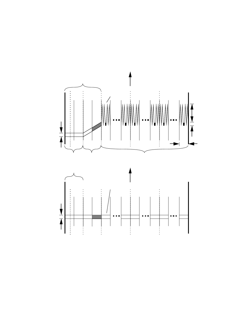
Figure 3. Cell types in a vertical division. The homeomorphism, $h^{-1}_{n}$, straightens the upper and lower boundaries of the cells.

If we are building horizontal cells, then all except the right most transition cells are $d_{n}$ by $a_{n}$ rectangles. The right most transition cells have a left boundary that is a straight line and a right boundary that is the left boundary of a Type 1 cell. See Figure 4.

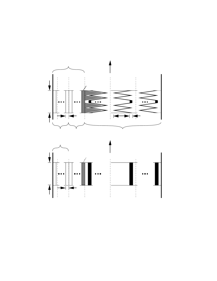
Figure 4. Various types of cells also occur in a horizontal division. The right most transition cell is shaded. No Type 2 cells are shown.

Type 1 cells are those that lie to the right of $\operatorname{Vert}(t_{n})$ that are not Type 2 cells. In general Type 2 cells are those that lie to the right of $\operatorname{Vert}(t_{n})$ and that lie along a hole $w_{n-1}\in W_{n-1}$. To be more specific we must consider the vertical and horizontal cases separately. When $n$ is odd, a Type 2 cell is a cell that either lies to the right of $\operatorname{Vert}(t_{n-5})$ and also lies along the vertical boundary of a hole $w_{n-1}\in W_{n-1}$ or lies between $\operatorname{Vert}(t_{n})$ and $\operatorname{Vert}(t_{n-5})$ and also shares a vertical boundary with another Type 2 cell. When $n$ is even, a Type 2 cell is one that lies to the right of $\operatorname{Vert}(t_{n-5})$ and also lies along the horizontal boundary of a hole $w_{n-1}\in W_{n-1}$. See Figure 5.

Figure 5. Type 2 cells occur alongside other Type 2 cells or alongside the holes $w_{n-1}\in W_{n-1}$ introduced in the previous iteration.

For vertical cells both Type 1 or Type 2 cells will consist of $k_{n}/2$ congruent pieces on the left joined by a rectangle of width $s_{n}$ to $k_{n}/2$ congruent pieces on the right. See Figure 6.

Figure 6. The two types of cells which occur to the right of $\operatorname{Vert}(t_{n})$ are Type 1 and Type 2 cells.

Such a cell will be symmetrical about a vertical line running through the center of the rectangle. Each of the $k_{n}$ pieces, which we call a cell-piece, will consist of two symmetrical parts called cell-points. Note that the width of a cell-piece is $(a_{n}-s_{n})/k_{n}$. In Type 1 cells the two cell-points of a cell-piece are congruent and “point” in the same direction. For a typical cell $q_{n}\in Q_{n}$ of Type 1 see Figure 6. Note that $a_{n}$ defines the width of $q_{n}$. The cell has a height of at least $c_{n}$ but less than $b_{n}+c_{n}$. The thickness; i.e., vertical transverse thickness, of the cell is limited by $b_{n}$. Horizontal cells are similar to vertical cells except they are rotated by ninety degrees.

For a typical vertical cell $q_{n}\in Q_{n}$ of Type 2 see Figure 6. Like Type 1 cells, $a_{n}$ defines the width of $q_{n}$ and the thickness of the cell is limited by $b_{n}$. In Type 2 cells, however, the two cell-points of a cell-piece will not in general be congruent nor will they “point” in the same direction. In addition the height of Type 2 cells can be greater than $c_{n}+b_{n}$ and in fact can have height greater than $2c_{n}+s_{n-1}$ where $s_{n-1}$ is the length of a side of the square holes in $W_{n-1}$. When a Type 2 cell lies along a hole in $W_{n-1}$, its cell-pieces are forced to extend at least $c_{n}/2$, but no more than $c_{n}+b_{n}$, beyond the hole. Note that, when $n$ is odd (respectively even), cells to the right of $\operatorname{Vert}(t_{n})$ that share a common vertical (respectively horizontal) boundary are congruent.

At stage $n$ the function $f_{n}$ will be defined so that eventually the elements of the decomposition that lie between $\operatorname{Vert}({t_{n-3}})$ and $\operatorname{Vert}({t_{n-4}})$ will be stretched vertically up close to the top edge of $D$ and down towards the bottom edge of $D$. Specifically, $f_{n}$ will be defined so that a horizontal line segment of length $a_{n}$ and lying between $\operatorname{Horiz}(2-a_{n})$ and $\operatorname{Horiz}(a_{n})$ and between $\operatorname{Vert}({t_{n-3}})$ and $\operatorname{Vert}({t_{n-4}})$ will be bent above $\operatorname{Horiz}(2-a_{n})$ and below $\operatorname{Horiz}(a_{n})$. For $n>3$ the function $f_{n}$ will be the identity to the right of $\operatorname{Vert}({t_{n-4}})$ and to the left of $\operatorname{Vert}({t_{n-3}})$. Between $\operatorname{Vert}(t_{n-3})$ and $\operatorname{Vert}(t_{n-4})$, $f_{n}$ is a homeomorphism from $[t_{n-3},t_{n-4}]\times[0,2]$ onto $[t_{n-3},t_{n-4}]\times[0,2]$ that maps vertical lines onto vertical lines and that is periodic in its first argument, the period being $a_{n}$. In addition $f_{n}$ between $\operatorname{Vert}(t_{n-3})$ and $\operatorname{Vert}(t_{n-4})$ satisfies the following constraints:

1. $f_{n}$ maps some point of the segment $[t_{n-3},t_{n-3}+\frac{a_{n}}{2}]\times\{a_{n}\}$ above $\operatorname{Horiz}(2-a_{n})$, and

2. $f_{n}$ maps some point of the segment $[t_{n-3}+\frac{a_{n}}{2},t_{n-3}+a_{n}]\times\{2-a_{n}\}$ below $\operatorname{Horiz}(a_{n})$.

See Figure 7.

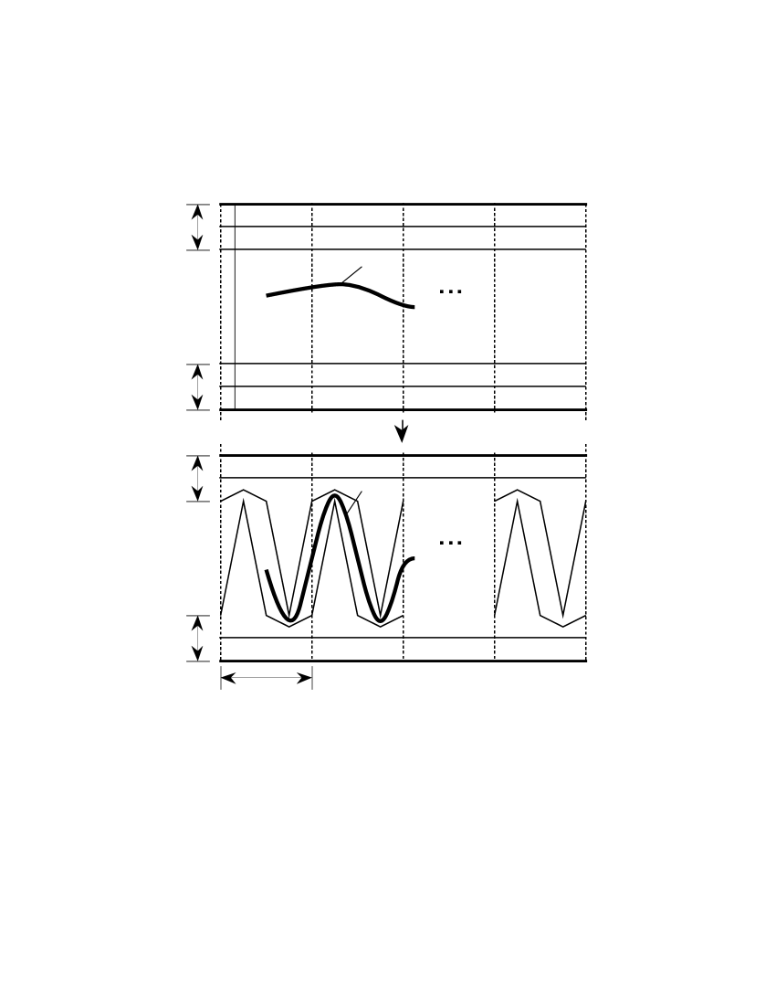
Figure 7. The definition of $f_{n}$.

We define ${f_{1}=f_{2}=f_{3}=\operatorname{Id}_{D}}$. Assuming that the sequence of functions $\{f_{n}\}_{n=1}^{\infty}$ has been defined we define ${F:(D\backslash E)\rightarrow(D\backslash E)}$ for every $x\in(D\backslash E)$ by the following equation when $x$ lies between $\operatorname{Vert}(t_{n})$ and $\operatorname{Vert}(t_{n-1})$:

$$F(x)=f_{n+3}\circ\cdot\cdot\cdot\circ f_{1}(x).$$

Thus $F$ is a homeomorphism. Once $f_{n}$ is defined we know how small the holes must be to keep them from getting stretched excessively by $f_{n}\circ f_{n-1}\circ\cdot\cdot\cdot\circ f_{1}$. We will only introduce these new holes to the right of $\operatorname{Vert}({t_{n-4}})$. See Figure 8.

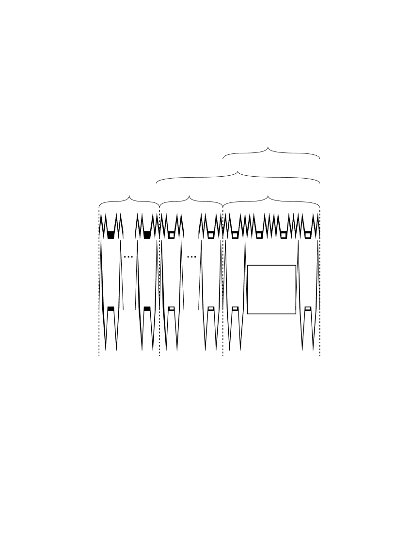
Figure 8. Holes are only introduced into cells in $Q_{n}$ to the right of $\operatorname{Vert}(t_{n-4})$.

4. The Construction

We now describe the construction in more detail. We assume we are at stage $n$ where $n>1$ and that we are given a division of $D$, $\widehat{R}_{n}$, and a continuum, $X_{n}\subset D$, which is essentially a rectangle minus a finite number of open squares with disjoint boundaries. The smallest holes; i.e., those removed during the last stage, will be those in $W_{n-1}$ and occur to the right of $\operatorname{Vert}(t_{n-5})$. To start, we refine $\widehat{R}_{n}$ to create $R_{n}$ letting $a_{n}=\operatorname{mesh}(\widehat{R}_{n})/4$ be the mesh of $R_{n}$. The size and position of the holes of $X_{n}$ will have been previously chosen carefully so that the edges of the holes will lie on the edges of the strips of $R_{n}$.

4.1. The Creation of $Q_{n}$

Our strategy in defining the cells of $Q_{n}$ will be to define a sequence of disjoint polygonal lines $\{L^{j}_{n}\}_{j=-1}^{m_{n}+1}$ which run horizontally across the vertical strips of $R_{n}$ when $n$ is odd and run vertically across the horizontal strips of $R_{n}$ when $n$ is even. When $L^{j}_{n}$ runs horizontally, then by $L^{j}_{n}(x)$ we will mean the $y$ such that $(x,y)\in L^{j}_{n}$. Similarly, when $L^{j}_{n}$ runs vertically, then $(L^{j}_{n}(y),y)\in L^{j}_{n}$. When $n$ is odd we will define the open cell $\widehat{q}_{i,j}$ for each $i\in 1,...,{\frac{1}{2a_{n}}}$ and $j\in 0,...,(m_{n}+1)$ as follows:

$$\widehat{q}_{i,j}=\{(x,y)\in D:(i-1)a_{n}<(x-\frac{1}{2})<ia_{n}\mbox{ and }L_{n}^{j-1}(x)<y<L_{n}^{j}(x)\}.$$

We define $Q_{n}$ to be the closure of the nonempty cells:

$$Q_{n}=\{\operatorname{Cl}(\widehat{q}_{i,j}):X_{n}\cap\widehat{q}_{i,j}\neq\emptyset\mbox{, }i\in 1,...,\frac{1}{2a_{n}}\mbox{ and }j\in 0,...,(m_{n}+1)\}.$$

When $n$ is even we define $Q_{n}$ in an analogous manner. Because our strategy for defining $\{L^{j}_{n}\}_{j=-1}^{m_{n}+1}$ is slightly different when $n$ is odd from when $n$ is even we discuss them separately.

4.1.1. $n$ is odd.

The lines $\{L^{j}_{n}\}_{j=-1}^{m_{n}+1}$ will be defined first between $\operatorname{Vert}(t_{n})$ and $\operatorname{Vert}(1)$, then between $\operatorname{Vert}(1/2)$ and $\operatorname{Vert}(t_{n+1})$, and finally between $\operatorname{Vert}(t_{n+1})$ and $\operatorname{Vert}(t_{n})$. Between $\operatorname{Vert}(t_{n})$ and $\operatorname{Vert}(1)$ we proceed as in [S1995]. Let $O_{n}$ be the ordinates of the top and bottom edges of the holes in $X_{n}$ along with $0$ and $2$. For $y\in O_{n}\backslash\{2\}$ we denote by $\operatorname{Nxt}(y)$ the least element of $O_{n}$ greater than $y$. Based on the same patterns as used in [S1995], we define for each $y\in O_{n}$ three polygonal lines: $\underline{M}^{y}_{n}$, $M^{y}_{n}$, $\overline{M}^{y}_{n}$. For each $y\in O_{n}\backslash\{2\}$ additional polygonal lines are added between $M^{y}_{n}$ and $M^{\operatorname{Nxt}(y)}_{n}$ so that

1. the resulting cells are like the Type 1 and Type 2 cells described above;

2. the number of rows of cells between $M^{y}_{n}$ and $M^{\operatorname{Nxt}(y)}_{n}$, which we will denote by $m_{y}$, is such that $(\operatorname{Nxt}(y)-y)/m_{y}$ is a constant, which we denote by $d_{n}$; and

3. the constant $d_{n}$ divides $2^{-(n+9)}$.

Details on how this is done are contained in [S1995]. We will in addition assume that $L^{0}_{n}(x)=\overline{M}^{0}_{n}(x)-b_{n}+d_{n}$ and that $L^{m_{n}}_{n}(x)=\underline{M}^{2}_{n}(x)+b_{n}-d_{n}$. Since $d_{n}<b_{n}$ this can be done by simply inserting these two additional polygonal lines where they are needed. Note that none of these polygonal lines intersect and so there is a natural order induced by where they intersect $\operatorname{Vert}(1)$. Let $m_{n}=2/d_{n}-2$. Reindex the lines in ascending order starting with $L^{-1}_{n}=0$ and ending with $L^{m_{n}+1}_{n}=2$.

For each $x\in[1/2,t_{n+1}]$ and for each $j\in\{-1,0,1,...,m_{n}+1\}$ we define $L^{j}_{n}(x)=(j+1)d_{n}$. For $x\in(t_{n+1},t_{n})$ we define

$$L^{j}_{n}(x)=\frac{L^{j}_{n}(t_{n})-L^{j}_{n}(t_{n+1})}{t_{n}-t_{n+1}}(x-t_{n+1})+L^{j}_{n}(t_{n+1}).$$

4.1.2. $n$ is even.

Again we define the polygonal lines between $\operatorname{Vert}(t_{n})$ and $\operatorname{Vert}(1)$ first. When $n>4$ we do this in two separate steps: first between $\operatorname{Vert}(t_{n-4})$ and $\operatorname{Vert}(1)$, and then between $\operatorname{Vert}(t_{n})$ and $\operatorname{Vert}(t_{n-4})$. We let $O_{n}$ be the abscissa of all the vertical boundaries of the holes in $X_{n}$ along with $t_{n-4}$ and $1$. Based on the same pattern as used in [S1995] we define for each $x\in O_{n}$ three polygonal lines: $\underline{M}^{x}_{n}$, $M^{x}_{n}$, $\overline{M}^{x}_{n}$. For all $x\in O_{n}\backslash\{1\}$ additional polygonal lines are added between $M^{x}_{n}$ and $M^{\operatorname{Nxt}(x)}_{n}$ so that

1. the resulting cells are like the Type 1 and Type 2 cells described above;

2. the number of columns of cells between $M^{x}_{n}$ and $M^{\operatorname{Nxt}(x)}_{n}$, which we will denote by $m_{x}$, is such that $(\operatorname{Nxt}(x)-x)/m_{x}$ is a constant, which we denote by $d_{n}$; and

3. the constant $d_{n}$ divides the following numbers $2^{-(n+9)}$, $(1-t_{n-4})$, $(t_{n-4}-t_{n})$, and $(t_{n}-1/2)$.

Let $m^{\prime}_{n}=((1-t_{n-4})/d_{n})-2$ and re-index these polygonal lines between $\operatorname{Vert}(1)$ and $\operatorname{Vert}(t_{n-4})$ starting on the right side with $L_{n}^{-1}=\operatorname{Vert}(1)$, and continuing left to $L_{n}^{m^{\prime}_{n}}=\overline{M}_{n}^{t_{n-4}}$ and $L_{n}^{m^{\prime}_{n}+1}=M_{n}^{t_{n-4}}$. Note that $M_{n}^{t_{n-4}}\neq\operatorname{Vert}(t_{n-4})$, that $M_{n}^{t_{n-4}}$ is just $\overline{M}^{t_{n-4}}_{n}$ shifted to the left by $b_{n}$, and that we are indexing the lines in reverse order with respect to that in [S1995]. We continue defining the polygonal lines between $\operatorname{Vert}(t_{n})$ and $\operatorname{Vert}(t_{n-4})$ by setting $L_{n}^{m^{\prime}_{n}+1+i}(y)=L_{m}^{m^{\prime}_{n}+1}(y)-i\cdot d_{n}$ for all $i\in\{1,2,...,(t_{n-4}-t_{n})/d_{n}\}$. Set $m^{\prime\prime}_{n}=m^{\prime}_{n}+(t_{n-4}-t_{n})/d_{n}$.

When $n\leq 4$ let $t^{\prime}=1-(a_{n-1}/2)$ and we again proceed in two separate steps: first between $\operatorname{Vert}(t^{\prime})$ and $\operatorname{Vert}(1)$, and then between $\operatorname{Vert}(t_{n})$ and $\operatorname{Vert}(t^{\prime})$. We let $O_{n}$ consist of $t^{\prime}$ and $1$. Based on the same pattern as used in [S1995] we define for each $x\in O_{n}$ three polygonal lines: $\underline{M}^{x}_{n}$, $M^{x}_{n}$, $\overline{M}^{x}_{n}$. For all $x\in O_{n}\backslash\{1\}$ additional polygonal lines are added between $M^{x}_{n}$ and $M^{\operatorname{Nxt}(x)}_{n}$ so that

1. the resulting cells are like the Type 1 cells described above;

2. the number of columns of cells between $M^{x}_{n}$ and $M^{\operatorname{Nxt}(x)}_{n}$, which we will denote by $m_{x}$, is such that $(\operatorname{Nxt}(x)-x)/m_{x}$ is a constant, which we denote by $d_{n}$; and

3. the constant $d_{n}$ divides the following numbers: $2^{-(n+9)}$, $a_{n-1}/2$, $(t^{\prime}-t_{n})$, and $(t_{n}-1/2)$.

Let $m^{\prime}_{n}=a_{n-1}/(2d_{n})-2$ and re-index these polygonal lines between $\operatorname{Vert}(1)$ and $\operatorname{Vert}(t^{\prime})$ starting on the right side with $L_{n}^{-1}=\operatorname{Vert}(1)$, and continuing left to $L_{n}^{m^{\prime}_{n}}=\overline{M}_{n}^{t^{\prime}}$ and $L_{n}^{m^{\prime}_{n}+1}=M_{n}^{t^{\prime}}$. We continue defining the polygonal lines between $\operatorname{Vert}(t_{n})$ and $\operatorname{Vert}(t^{\prime})$ by setting $L_{n}^{m^{\prime}_{n}+1+i}(y)=L_{m}^{m^{\prime}_{n}+1}(y)-i\cdot d_{n}$ for all $i\in\{1,2,...,(t^{\prime}-t_{n})/d_{n}\}$. Set $m^{\prime\prime}_{n}=m^{\prime}_{n}+(t^{\prime}-t_{n})/d_{n}$.

Once we have defined all the polygonal lines between $\operatorname{Vert}(t_{n})$ and $\operatorname{Vert}(1)$ we define the polygonal lines between $\operatorname{Vert}(1/2)$ and $\operatorname{Vert}(t_{n})$ by setting $L_{n}^{m^{\prime\prime}_{n}+1+i}(y)=t_{n}-i\cdot d_{n}$ for all $i\in\{1,2,...,(t_{n}-1/2)/d_{n}\}$. Set $m_{n}=m^{\prime\prime}_{n}+((t_{n}-1/2)/d_{n})$.

4.2. Definition of the Homeomorphisms

We define $h_{n}:D\rightarrow D$ to be a homeomorphism which maps vertical lines when $n$ is odd and horizontal lines when $n$ is even onto themselves each in a piecewise linear manner so that the preimage of the polygonal arcs $\{L^{j}_{n}\}_{j=-1}^{m_{n}+1}$ is a collection of parallel straight lines evenly spaced apart at the distance $d_{n}$. Thus $h^{-1}_{n}(Q_{n})$ is a collection of rectangles with disjoint interiors. Note that $h_{n}$ is the identity between $\operatorname{Vert}(1/2)$ and $\operatorname{Vert}(t_{n+1})$. Also, note that because of the way the polygonal arcs $\{L^{j}_{n}\}_{j=-1}^{m_{n}+1}$ were defined, $h_{n}$ maps the boundary of each hole of $X_{n}$ onto itself. Thus, if $w_{i}\in W_{i}$, then $h_{n}(\operatorname{Cl}(w_{i}))=\operatorname{Cl}(w_{i})$ for all $i<n$.

When $n$ is even there is another important result that follows from the way the polygonal arcs $\{L^{j}_{n}\}_{j=-1}^{m_{n}+1}$ are defined; namely, that $\operatorname{Width}(x,h_{n}(x))<2a_{n-1}$. This follows from the way the parameters $a_{n}$, $b_{n}$, $c_{n}$ are chosen and from the following observations. When $n>4$, then to the right of $\operatorname{Vert}(t_{n-4})$ both $h^{-1}_{n}(L^{i}_{n})$ and $L^{i}_{n}$ either intersect the same column of holes in $W_{n-1}$ or they are both between two columns of holes from $W_{n-1}$ that are spaced no further than $a_{n-1}$ apart. If $h_{n}^{-1}(L_{n}^{i})$ is to the left of $\operatorname{Vert}(t_{n-4})$, then $h_{n}^{-1}(L_{n}^{i})\cap L_{n}^{i}\neq\emptyset$. Similarly when $n\leq 4$, either $h_{n}^{-1}(L_{n}^{i})\cap L_{n}^{i}\neq\emptyset$ or both $h_{n}^{-1}(L_{n}^{i})$and $L_{n}^{i}$ are between $\operatorname{Vert}(1-a_{n-1}/2)$ and $\operatorname{Vert}(1)$.

As in the constructions described in [S1994, S1995] the map $h_{n}$ can cause a great deal of stretching of cells that lie along the horizontal edge of a hole (or $D$) when $n$ is odd or along a vertical edge of a hole (or $D$) when $n$ is even. If we are not careful, this stretching could potentially cause holes introduced at stage $n$ to be overly enlarged or to be too widely separated. In an approach analogous to that described in [S1994, S1995] we control where this stretching can occur in order to avoid problems. We force it to occur at a distance between $a^{\prime}_{n}/128$ and $a^{\prime}_{n}/64$ from the horizontal (vertical) boundary of $X_{n}$ when $n$ is odd (even). When $n$ is odd $h_{n}$ is the identity below than $\operatorname{Horiz}(a^{\prime}_{n}/128)$ and above $\operatorname{Horiz}(2-a^{\prime}_{n}/128)$. There is another place where $h_{n}$ can cause a great deal of stretching and that is among the transition cells. Note that in this case holes are only added to the transition cells at a much later stage and that then the exact amount of stretching is known and the holes can be made appropriately small and close together. We define $H_{n}$ to be $h_{1}\circ\cdot\cdot\cdot\circ h_{n-1}$ when $n>1$ and $H_{1}$ to be $\operatorname{Id}_{D}$. Thus $Y_{1}=H_{1}(X_{1})=D$ and $P_{1}=H_{1}(Q_{1})=Q_{1}$.

4.3. Preparation of the Next Stage

We will set

$$P_{n}=H_{n}(Q_{n})\mbox{\quad and \quad}Y_{n}=H_{n}(X_{n}).$$

To continue the construction, we set

$$W^{\prime}_{n}=\{w_{n}:\exists q_{n}\in Q_{n}\mbox{ and }w_{n}\mbox{ is an open }s_{n}\mbox{ by }s_{n}\mbox{ square centered in }h_{n}^{-1}(q_{n})\}.$$

We define $W_{1}=W_{2}=W_{3}=\emptyset$ and for $n>3$ we set

$$W_{n}=W^{\prime}_{n}\cap([t_{n-4},1]\times[0,2]).$$

Define

$$X_{n+1}=X_{n}\backslash W^{*}_{n}.$$

This definition of $X_{n+1}$ prevents us from removing any holes to the left of $\operatorname{Vert}(t_{n-4})$. The next division $\widehat{R}_{n+1}$ is derived from projecting the vertices of the rectangles $h^{-1}_{n}(Q_{n})$ onto the $y$-axis if $n$ is odd and onto the $x$-axis if $n$ is even. Note that $\operatorname{mesh}(\widehat{R}_{n+1})=d_{n}$.

5. The Specific Construction

We will now apply the construction to build the continuum $Y=\cap_{n=1}^{\infty}Y_{n}$ and the collection $G=\{\cap_{n=1}^{\infty}\operatorname{st}(p_{n},P_{n})^{*}:\cap_{n=1}^{\infty}p_{n}\neq\emptyset\mbox{ where }p_{n}\in P_{n}\}$ of subsets of $Y$. We first describe exactly how the parameters that control the construction are chosen. Assuming we are at stage $n$ the parameters are chosen in the order given below. The sequences $\{L_{i}\}_{i=-1}^{\infty}$ and $\{K_{i}\}_{i=-1}^{\infty}$ are used to control the size of the elements of the decomposition $G$.

1. Let $t_{n}={1/2}+(1/2)^{n+1}$ with $t_{0}=1$.

2. Let $a_{n}=a^{\prime}_{n-1}$ with $a_{1}=(1/2)^{33}$.

3. Let $c_{n}=a_{n-1}/9$ with $c_{1}=(1/2)^{25}$.

4. Let $L_{n}=a_{n}/24$ with $L_{0}=L_{-1}=1/128$.

5. Let $K_{n}=4L_{n}$.

6. Define $f_{n}$ as described above so that between $\operatorname{Vert}(t_{n-3})$ and $\operatorname{Vert}(t_{n-4})$ a horizontal line segment that lies between $\operatorname{Horiz}(a_{n})$ and $\operatorname{Horiz}(2-a_{n})$ that is of width $a_{n}$ gets bent above $\operatorname{Horiz}(2-a_{n})$ and below $\operatorname{Horiz}(a_{n})$. Note that $f_{1}=f_{2}=f_{3}=\operatorname{Id}_{D}$. As above define $F:(Y_{1}\backslash E)\rightarrow(Y_{1}\backslash E)$ by $F(x)=f_{n}\circ\cdot\cdot\cdot\circ f_{1}(x)$ if $x$ is between $\operatorname{Vert}(t_{n-3})$ and $\operatorname{Vert}(t_{n-4})$ for $n>3$.

7. Let $\delta_{n}>0$ so that

   1. $|x-x^{\prime}|<\delta_{n}\implies|H_{n}(x)-H_{n}(x^{\prime})|<L_{n}/2^{n+1}$, and

   2. $|x-x^{\prime}|<\delta_{n}\implies|f_{n}\circ\cdot\cdot\cdot\circ f_{1}\circ H_{n}(x)-f_{n}\circ\cdot\cdot\cdot\circ f_{1}\circ H_{n}(x^{\prime})|<(1/2)^{n+1}$.

8. Let $b_{n}>0$ be rational so that

   1. $b_{n}<\delta_{n}/4$,

   2. $b_{n}<a_{n}/(2k_{n-1})$ where $k_{0}=512$,

   3. $b_{n}<b_{n-1}(a_{n-1}-s_{n-1})/(4k_{n-1}(c_{n-1}+b_{n-1}))$ when $n>1$, and

   4. $b_{n}<a_{n}/2^{n+6}$.

9. Define $m_{n}$ and $d_{n}$ as in 4.1. Recall that we will have

   1. $d_{n}\mbox{ divides }(1/2)^{n+9}$ and $d_{n}\mbox{ divides }a_{n-1}/2$.

10. Define $h_{n}$ as in 4.2. Define $H_{n}=h_{1}\circ\cdot\cdot\cdot\circ h_{n-1}$ with $H_{1}=\operatorname{Id}_{D}$.

11. Let $a^{\prime}_{n}=d_{n}/4$ and $s_{n}=2a^{\prime}_{n}=d_{n}/2$.

12. Let $k_{n}$ be an integer so that

    1. $k_{n}\geq 512$,

    2. $4\mbox{ divides }k_{n}$, and

    3. $k_{n}>a_{n}/a^{\prime}_{n}$.

It can be shown as in [S1995] that at each stage $n$ we can pick $a_{n}$, $a^{\prime}_{n}$, $b_{n}$, $c_{n}$, $s_{n}$, and $k_{n}$ following the above constraints so that it is possible to continue the construction to stage $n+1$. We must also be able to show that

1. the continuum $Y=\cap_{n=1}^{\infty}Y_{n}$ is the Sierpiński curve;

2. the continuum $F(Y\backslash E)\cup E$ is the Sierpiński curve;

3. all members of $G$ except those that intersect the left edge of $D$ are nondegenerate;

4. the collection $G=\{\cap_{n=1}^{\infty}\operatorname{st}(p_{n},P_{n})^{*}:\cap_{n=1}^{\infty}p_{n}\neq\emptyset\mbox{ where }p_{n}\in P_{n}\}$ is a continuous decomposition of $Y$.

5. the collection $G^{\prime}=\{F(g)|g\in G\mbox{ and }g\cap E=\emptyset\}\cup\{E\}$ is a continuous decomposition of $F(Y\backslash E)\cup E$; and

6. the decomposition space $(F(Y\backslash E)\cup E)/G^{\prime}$ is homeomorphic to the Sierpiński curve.

We can show that 1–4 above hold in precisely the same way as they are shown in [S1995]. To show 5–6 we need the following lemma. It guarantees that every $g\in G$ will be bent and sufficiently stretched vertically by $F$.

Lemma 5.1.

Let $g\in G$ and let $n$ be the least integer such that $g$ is strictly to the right of $\operatorname{Vert}(t_{n+1})$. Let $g=\cap_{i=1}^{\infty}\operatorname{st}(p_{i},P_{i})^{*}$ where $p_{i}\in P_{i}$ for all $i\in\operatorname{\mathbb{Z}}^{+}$ and $\cap_{i=1}^{\infty}p_{i}\neq\emptyset$. Let $q_{i}=H^{-1}_{i}(p_{i})$ for all $i$. Assume $n>4$.

If $p_{n-1}\cap\operatorname{Vert}(t_{n+1})=\emptyset$, then there exists a trapezoid $T$ between $\operatorname{Vert}(t_{n+1})$ and $\operatorname{Vert}(t_{n-1})$ so that

1. $\operatorname{Width}(T)>a_{n+3}$,

2. if $(x,y)\in T$, then $a_{n+3}<y<2-a_{n+3}$,

3. every vertical line that intersects $T$ will intersect $g\cap T$;

and

if $p_{n-1}\cap\operatorname{Vert}(t_{n+1})\neq\emptyset$, then there exists a trapezoid $T$ between $\operatorname{Vert}(t_{n+1})$ and $\operatorname{Vert}(t_{n})$ so that

1. $\operatorname{Width}(T)>a_{n+4}$,

2. if $(x,y)\in T$, then $a_{n+4}<y<2-a_{n+4}$,

3. every vertical line that intersects $T$ will intersect $g\cap T$;

Proof.

Since $H_{n-1}=\operatorname{Id}_{D}$ to the left of $\operatorname{Vert}(t_{n-1})$ it can be shown that $p_{n-1}=q_{n-1}$ because of the definition of $n$. Since $p_{n-1}$ must be between $\operatorname{Vert}(t_{n+1})$ and $\operatorname{Vert}(t_{n-1})$, we know that for any $m\in\operatorname{\mathbb{Z}}^{+}$ there some point of $p_{n+m}$ that lies between $\operatorname{Vert}(t_{n+1})$ and $\operatorname{Vert}(t_{n-1})$. Thus for any $m\in\operatorname{\mathbb{Z}}^{+}$ we have that $q_{n+m}$ is strictly to the right of $\operatorname{Vert}(t_{n+2})$. (See, for example, the proof of Lemma 9 of [S1998]). Applying Claim C of [S1998] we have that for all $m\geq n$

$$p_{m+3} \subset \operatorname{st}(p_{m+4-1},P_{m+4-1})^{*}$$

$$\subset \sideset{}{{}_{\frac{12L_{m+2}+3K_{m+2}}{2^{m+4}}}}{\operatorname{N}}(g)$$

$$\subset \sideset{}{{}_{\frac{a_{m+2}}{2^{m+4}}}}{\operatorname{N}}(g).$$

First we assume that $p_{n-1}\cap\operatorname{Vert}(t_{n+1})=\emptyset$. If $g$ lies between $\operatorname{Horiz}(a_{n+3})$ and $\operatorname{Horiz}(2-a_{n+3})$, then we are done because it can be shown that $\operatorname{Width}(g)>a_{n+3}$. See, for example, the proof of Lemma 10 in [S1998]. So assume that there is a point $x\in g$ that is below $\operatorname{Horiz}(a_{n+3})$. The situation when there is a point $x\in g$ that is above $\operatorname{Horiz}(2-a_{n+3})$ is handled similarly.

Case $1$: Assume that $n$ is odd in addition to assuming $p_{n-1}\cap\operatorname{Vert}(t_{n+1})=\emptyset$. Since $g\subset\operatorname{st}(p_{n+1},P_{n+1})^{*}$ there is a $\widehat{p}_{n+1}\in\operatorname{st}(p_{n+1},P_{n+1})$ so that $x\in\widehat{p}_{n+1}$. Note that $\widehat{q}_{n+1}=H^{-1}_{n+1}(\widehat{p}_{n+1})$ is a horizontal cell since $n+1$ is even. Because of the way polygonal lines were defined, specifically that $L^{0}_{n}(x)=\overline{M}^{0}_{n}(x)-b_{n}+d_{n}$ and that $L^{m_{n}}(x)_{n}=\underline{M}^{2}_{n}+b_{n}-d_{n}$, we know that $h_{n}$ is the identity below $\operatorname{Horiz}(d_{n})$ and above $\operatorname{Horiz}(2-d_{n})$ between $\operatorname{Vert}(t_{n+1})$ and $\operatorname{Vert}(t_{n})$ and because of the way stretching is controlled near boundaries we know that $h_{n}$ is the identity below $\operatorname{Horiz}(a_{n+1}/128)$. Note that $h_{n-1}$ is the identity to the left of $\operatorname{Vert}(t_{n}+3d_{n-1})$. Thus since $x$ is below $horiline(a_{n+3})$, we have that $H^{-1}_{n+1}(x)$ and that $x\in\widehat{q}_{n+1}$. Let $\widehat{q}^{p}_{n+1}$ be a cell-piece of the cell $\widehat{q}_{n+1}$ that lies between $\operatorname{Horiz}(a_{n+1}/128)$ and $\operatorname{Horiz}(a_{n+1}/256)$. Such a cell-piece exists since $k_{n+1}\geq 512$ and the width of a cell-piece is $(a_{n+1}-s_{n+1})/k_{n+1}$. Let $\ell_{1}$ and $\ell_{2}$ be the horizontal lines that run along the top and bottom boundaries of $\widehat{q}^{p}_{n+1}$ respectively. Define $T^{\prime}$ to be the part of $\operatorname{st}(q_{n+1},Q_{n+1})^{*}$ that lies between $\ell_{1}$ and $\ell_{2}$. Notice that since $a_{n+3}<a_{n+1}/256$, $x$ is below $\ell_{2}$. See Figure 9.

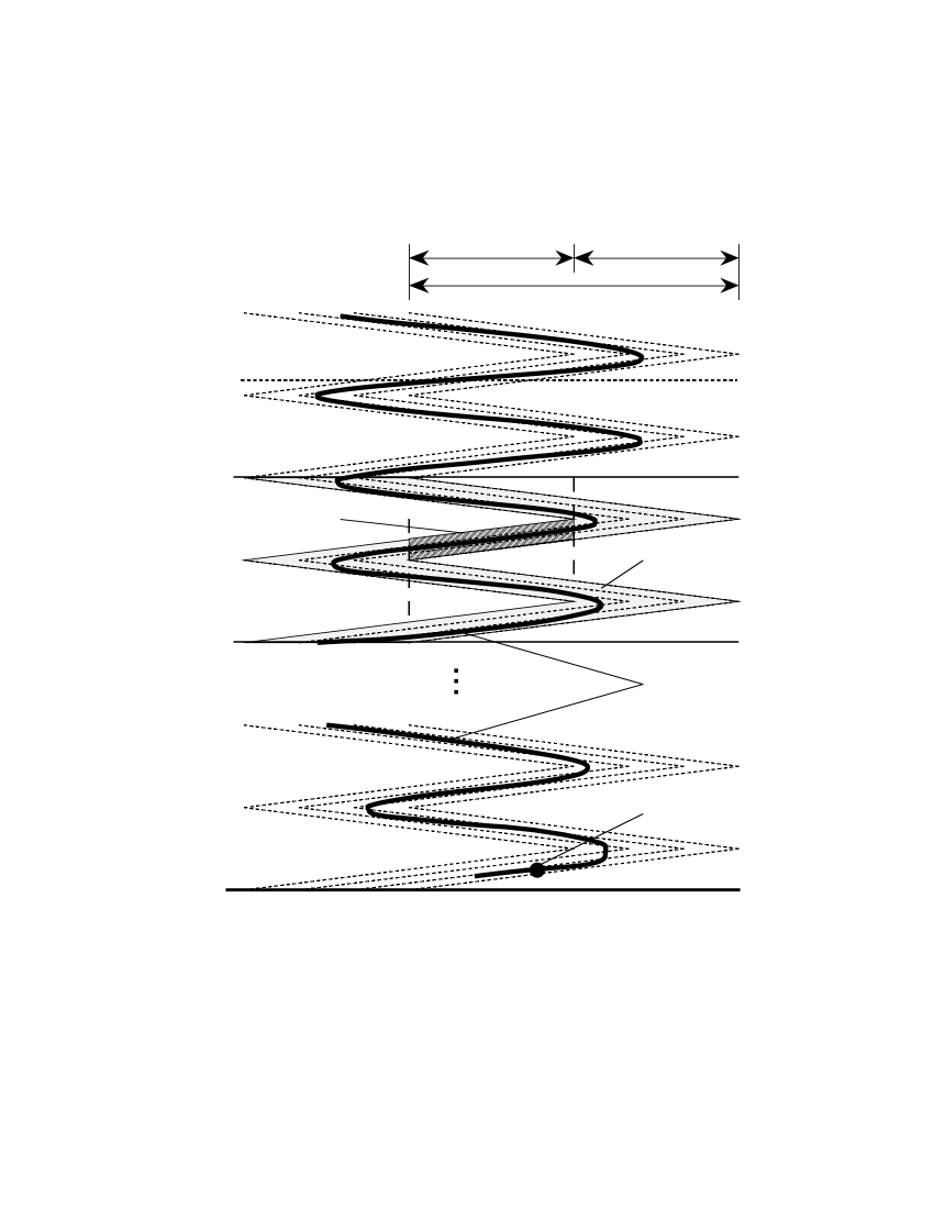
Figure 9. Case 1 of Lemma 5.1.

Now $H_{n+1}(T^{\prime})=H_{n-1}\circ h_{n-1}\circ h_{n}(T^{\prime})=T^{\prime}$, and $T^{\prime}\subset\operatorname{st}(p_{n+1},P_{n+1})^{*}$.

Consider $p_{n+3}$. There is $q^{\prime}_{n+2}\in\operatorname{st}(q_{n+2},Q_{n+2})$ so that $q_{n+3}$ crosses some cell-point of $q^{\prime}_{n+2}$. But $c_{n+2}=a_{n+1}/9>a_{n+1}/64$ so some point of $p_{n+3}$ lies above $\operatorname{Horiz}(a_{n+1}/64)$ and since $a_{n+2}/2^{n+2}<a_{n+1}/128$ we can conclude from Equation 5 that some point of $g$ lies above $\ell_{1}$. Therefore $g$ must lie along $T^{\prime}$ and “cross” one of the “cell points” of $T^{\prime}$. Now $c_{n+1}-3b_{n+2}>a_{n+3}$ so there exists a trapezoid $T\subset T^{\prime}$ that satisfies conditions 1–3.

Case $2$: Assume $n$ is even in addition to assuming $p_{n-1}\cap\operatorname{Vert}(t_{n+1})=\emptyset$. Consider $\widehat{p}_{n+2}\in\operatorname{st}(p_{n+2},P_{n+2})$ so that $x\in\widehat{p}_{n+2}$. Note that $\widehat{q}_{n+2}=H^{-1}_{n+2}(\widehat{p}_{n+2})$ is a horizontal cell. If $q^{\prime}_{n+2}\in\operatorname{st}(q_{n+2},Q_{n+2})$ then denote $H_{n+2}(q^{\prime}_{n+2})$ by $p^{\prime}_{n+2}$. Since $H_{n-2}$ is the identity to the left of $\operatorname{Vert}(t_{n-2})$ we have that $p^{\prime}_{n+2}=h_{n-1}\circ h_{n}\circ h_{n+1}(q^{\prime}_{n}+2)$. Now $h_{n+1}$ is the identity below $\operatorname{Horiz}(a_{n+2}/128)$. Also we know that $h_{n-1}$ is the identity below $\operatorname{Horiz}(d_{n-1})$ and to the left of $\operatorname{Vert}(t_{n-1})$. Recall that $d_{n-1}>a_{n+1}/128$. Finally, because $h_{n}$ maps horizontal lines onto horizontal lines and because the image under $h_{n}$ of any point of $\operatorname{st}(q_{n+2},Q_{n+2})$ is to the left of $\operatorname{Vert}(t_{n-1})$, we can conclude that $H_{n+2}(q^{\prime}_{n+2})=h_{n}(q^{\prime}_{n+2})$ and that $h^{-1}_{n}(x)\in\widehat{q}_{n+2}$ which is below $a_{n+3}$. Let $\widehat{q}^{p}_{n+2}$ be a cell-piece of the cell $\widehat{q}_{n+2}$ that lies between $\operatorname{Horiz}(a_{n+2}/128)$ and $\operatorname{Horiz}(a_{n+2}/256)$. Let $\ell_{1}$ and $\ell_{2}$ be the horizontal lines that run along the top and bottom boundaries of $\widehat{q}^{p}_{n+2}$ respectively. Define $T^{\prime}$ to be the part of $\operatorname{st}(q_{n+2},Q_{n+2})^{*}$ that lies between $\ell_{1}$ and $\ell_{2}$. Notice that since $a_{n+3}<a_{n+2}/256$, $x$ is below $\ell_{2}$ and that $H_{n+2}(T^{\prime})=h_{n}(T^{\prime})$. Again from Equation 5 and the fact that $c_{n+3}>a_{n+2}/64$ we can conclude that some point of $g$ lies above $\ell_{1}$ and that $g$ is forced to lie along the image under $h_{n}$ of a “cell-piece” of $T^{\prime}$. Because of the behavior of $h_{n}$ to the left of $\operatorname{Vert}(t_{n-1})$ we can find a trapezoid $T\subset h_{n}(T^{\prime})$ that satisfies conditions 1–3 of the lemma.

Now we will assume that $p_{n-1}\cap\operatorname{Vert}(t_{n+1})\neq\emptyset$. We also assume that there is a point $x\in g$ that is below $\operatorname{Horiz}(a_{n+4})$. The situation when $x$ is close to the top boundary of $D$ is handled similarly.

Case $1^{\prime}$: Assume that $n$ is odd in addition to assuming $p_{n-1}\cap\operatorname{Vert}(t_{n+1})\neq\emptyset$. Consider $\widehat{p}_{n+3}\in\operatorname{st}(p_{n+3},P_{n+3})$ so that $x\in\widehat{p}_{n+3}$. Note that $\widehat{q}_{n+3}=H^{-1}_{n+3}(\widehat{p}_{n+3})$ is a horizontal cell. If $q^{\prime}_{n+3}\in\operatorname{st}(q_{n+3},Q_{n+3})$ then denote $H_{n+3}(q^{\prime}_{n+3})$ by $p^{\prime}_{n+3}$. Since $H_{n}$ is the identity to the left of $\operatorname{Vert}(t_{n})$ we have that $p^{\prime}_{n+3}=h_{n}\circ h_{n+1}\circ h_{n+2}(q^{\prime}_{n}+3)$. As in Case 1 above we see that $h_{n+2}$ is the identity below $\operatorname{Horiz}(a_{n+3}/128)$. Also we know that $h_{n}$ is the identity below $\operatorname{Horiz}(d_{n})$ and to the left of $\operatorname{Vert}(t_{n})$. Finally because $h_{n+1}$ maps horizontal lines onto horizontal lines and because the image under $h_{n+1}$ of any point of $h_{n+2}(\operatorname{st}(q_{n+3},Q_{n+3}))$ is to the left of $\operatorname{Vert}(t_{n})$ we can conclude that $H_{n+3}(q^{\prime}_{n+3})=h_{n+1}(q^{\prime}_{n+3})$ and that $h^{-1}_{n+1}(x)\in\widehat{q}_{n+3}$ which is below $a_{n+4}$. Let $\widehat{q}^{p}_{n+3}$ be a cell-piece of the cell $\widehat{q}_{n+3}$ that lies between $\operatorname{Horiz}(a_{n+3}/128)$ and $\operatorname{Horiz}(a_{n+3}/256)$. Let $\ell_{1}$ and $\ell_{2}$ be the horizontal lines that run along the top and bottom boundaries of $\widehat{q}^{p}_{n+3}$ respectively. Define $T^{\prime}$ to be the part of $\operatorname{st}(q_{n+3},Q_{n+3})^{*}$ that lies between $\ell_{1}$ and $\ell_{2}$. Notice that since $a_{n+4}<a_{n+3}/256$, $x$ is below $\ell_{2}$, and that $H_{n+3}(T^{\prime})=h_{n+1}(T^{\prime})$. From Equation 5 and the fact that $c_{n+4}>a_{n+3}/64$ we can conclude that some point of $g$ lies above $\ell_{1}$ and that $g$ is forced to lie along the image under $h_{n+1}$ of a “cell-piece” of $T^{\prime}$. Because of the behavior of $h_{n+1}$ near $\operatorname{Vert}(t_{n+1})$ we can find a rectangle $T\subset h_{n+1}(T^{\prime})$ that satisfies conditions $1^{\prime}$–$3^{\prime}$ of the lemma.

Case $2^{\prime}$: Assume $n$ is odd in addition to assuming $p_{n-1}\cap\operatorname{Vert}(t_{n+1})\neq\emptyset$. Exactly as in Case 2 above. ∎

We now observe that because $G$ is a continuous decomposition and the elements of $G$ that intersect the left edge of $D$ are singletons, the elements of $G$ have smaller and smaller diameters as they get closer to $E$. Because of the definition of $F$ for each $g\in G$ with $g\cap E=\emptyset$ we have that $\operatorname{Width}(g)=\operatorname{Width}(F(g))$. Thus the elements $g^{\prime}\in G^{\prime}$ have a smaller and smaller width as they get closer and closer to $E$.

Lemma 5.2.

The collection $G^{\prime}=\{F(g):g\in G\mbox{ and }g\cap E=\emptyset\}\cup\{E\}$ is a continuous decomposition of $Y^{\prime}=F(Y\backslash E)\cup E$.

Proof.

Since we have that $G$ is a continuous decomposition of $Y$ and that $F|(Y\backslash E)$ is a homeomorphism, then $G^{\prime}$ must be continuous at every $g^{\prime}\in G^{\prime}$ except possibly when $g^{\prime}=E$. But the Lemma 5.1 guarantees that the elements of $G^{\prime}$ get bent along $E$ so $G^{\prime}$ is lower semicontinuous at $E$ and by the argument preceding this lemma we have that $G^{\prime}$ is upper semicontinuous at $E$. Thus $G^{\prime}$ is continuous at $E$ also. ∎

Lemma 5.3.

The set $Y^{\prime}/G^{\prime}$ is the Sierpiński curve.

Proof.

Let $\pi:Y^{\prime}\rightarrow Y^{\prime}/G^{\prime}$ be the natural projection. We know that $Y^{\prime}/G^{\prime}$ is locally connected because $Y^{\prime}$ is. Since $G^{\prime}$ is upper semicontinuous, we know that by adding the points of the compliment of $Y^{\prime}$, we get an upper semicontinuous decomposition of ${\operatorname{\mathbb{E}}}^{2}$ which we will call $G^{\prime\prime}$. Thus we extend $\pi$ to $\widehat{\pi}:{\operatorname{\mathbb{E}}}^{2}\rightarrow{\operatorname{\mathbb{E}}}^{2}/G^{\prime\prime}$. No member of $G^{\prime\prime}$ separates the plane so by R.L. Moore’s Theorem [D1986] we know that ${\operatorname{\mathbb{E}}}^{2}/G^{\prime\prime}$ is homeomorphic to the plane. Thus $Y^{\prime}/G^{\prime}$ is planar. By Corollary 13 in [S1998], we get that $(\widehat{\pi})|\operatorname{Cl}(U)$ is a homeomorphism for any $U$ a bounded component of $(Y^{\prime})^{c}$. Finally, if $V$ is the unbounded component of $(Y^{\prime})^{c}$, then $\widehat{\pi}(\operatorname{Bd}(V))$ is also a simple closed curve. Thus the images under $\widehat{\pi}$ of the boundaries of the components of $(Y^{\prime})^{c}$ are simple closed curves, are dense in $Y^{\prime}/G^{\prime}$, and have diameters that go to zero. Therefore $Y^{\prime}/G^{\prime}$ is homeomorphic to the Sierpiński curve by [W1958]. ∎

This proves Theorem 2.1.

References

- [D1986] R. J. Daverman, Decompositions of Manifolds, Academic Press, New York, 1986.
- [L1978] W. Lewis and J. J. Walsh, A continuous decomposition of the plane into pseudo-arcs, Houston J. Math., 4 (1978), 209–222.
- [P1998] J. R. Prajs, Continuous decompositions of Peano plane continua into pseudo-arcs, Fund. Math. 158 (1998), no. 1, 23–40.
- [P1999] J. R. Prajs, Private communication, 1999.
- [S1994] C. R. Seaquist, A new continuous cellular decomposition of the disk into non-degenerate elements, Top. Proc., 19 (1994), 249–276.
- [S1995] C. R. Seaquist, A continuous decomposition of the Sierpiński curve, Continua with the Houston Problem Book, Edited by H. Cook, W.T. Ingram, K. Kuperberg, A. Lelek, P. Minc, (Marcel Dekker, New York, 1995), 315–342.
- [S1998] C. R. Seaquist, Monotone homogeneity of the Sierpiński curve, Top. Proc., (To appear).
- [W1958] G. T. Whyburn, Topological characterization of the Sierpiński curve, Fund. Math., 45 (1958), 320–324.