A polytope related to empirical distributions, plane trees, parking functions, and the associahedron

Abstract

The volume of the $n$-dimensional polytope

$$\Pi_{n}({\mbox{\boldmath$x$}}):=\{{\mbox{\boldmath$y$}}\in\mathbb{R}^{n}:y_{i}\geq 0\mbox{ and }y_{1}+\cdots+y_{i}\leq x_{1}+\cdots+x_{i}\mbox{ for all }1\leq i\leq n\}$$

for arbitrary ${\mbox{\boldmath$x$}}:=(x_{1},\ldots,x_{n})$ with $x_{i}>0$ for all $i$ defines a polynomial in variables $x_{i}$ which admits a number of interpretations, in terms of empirical distributions, plane partitions, and parking functions. We interpret the terms of this polynomial as the volumes of chambers in two different polytopal subdivisions of $\Pi_{n}({\mbox{\boldmath$x$}})$. The first of these subdivisions generalizes to a class of polytopes called sections of order cones. In the second subdivision, the chambers are indexed in a natural way by rooted binary trees with $n+1$ vertices, and the configuration of these chambers provides a representation of another polytope with many applications, the associahedron.

Key words and phrases. plane tree, Catalan numbers, Steck determinant, uniform order statistics, Minkowski sum, Ehrhart polynomial, mixed lattice point enumerator, depth-first search, plane partition, associahedron

AMS 1991 subject classification. Primary: 52B12, Secondary: 06A07, 05C05,62G30

1 Introduction

The focal point of this paper is the $n$-dimensional polytope

$$\Pi_{n}({\mbox{\boldmath$x$}}):=\{{\mbox{\boldmath$y$}}\in\mathbb{R}^{n}:y_{i}\geq 0\mbox{ and }y_{1}+\cdots+y_{i}\leq x_{1}+\cdots+x_{i}\mbox{ for all }1\leq i\leq n\}$$

for arbitrary ${\mbox{\boldmath$x$}}:=(x_{1},\ldots,x_{n})$ with $x_{i}>0$ for all $i$. The $n$-dimensional volume

$$V_{n}({\mbox{\boldmath$x$}}):=\mathrm{Vol}(\Pi_{n}({\mbox{\boldmath$x$}}))$$

is a homogeneous polynomial of degree $n$ in the variables $x_{1},\ldots,x_{n}$, which we call the volume polynomial. This polynomial arises naturally in several different settings: in the calculation of probabilities derived from empirical distribution functions or the order statistics of $n$ independent random variables (see §2), and in the study of parking functions and plane partitions (see §5). See also Marckert and Chassaing [15] regarding similar connections between the theories of parking functions, empirical processes, and rooted trees.

Trivially, $V_{1}({\mbox{\boldmath$x$}})=x_{1}$. The formula

$$V_{2}({\mbox{\boldmath$x$}})=x_{1}x_{2}+{\textstyle\frac{1}{2}}x_{1}^{2}$$

has two natural interpretations by a subdivision of $\Pi_{2}({\mbox{\boldmath$x$}})$ into 2 pieces of areas $x_{1}x_{2}$ and ${\textstyle\frac{1}{2}}x_{1}^{2}$, as shown in Figure 1 for horizontal coordinate $x_{1}=1$ and vertical coordinate $x_{2}=2$.

Figure 1: $\Pi_{2}({\mbox{\boldmath$x$}})$ and its two subdivisions

The 5 terms of

$$V_{3}({\mbox{\boldmath$x$}})=x_{1}x_{2}x_{3}+{\textstyle\frac{1}{2}}x_{1}^{2}x_{2}+{\textstyle\frac{1}{2}}x_{1}x_{2}^{2}+{\textstyle\frac{1}{2}}x_{1}^{2}x_{3}+{\textstyle\frac{1}{6}}x_{1}^{3}$$ (1)

can be interpreted in two ways as the volumes determined by two different subdivisions of $\Pi_{3}({\mbox{\boldmath$x$}})$ into 5 chambers, as in the perspective diagrams of Figure 2 where $x_{i}=i$ for $i=1,2,3$, the first coordinate points out of the page, the second to the right and the third up, and the viewpoint is $(5,-2,4)$.

Figure 2: $\Pi_{3}({\mbox{\boldmath$x$}})$ and its two subdivisions

A central result of this paper is the general formula for the volume polynomial which we present in the following theorem. Section 2 offers a simple probabilistic proof of this theorem. We show in Section 4 how this argument can also be interpreted geometically by a subdivision of $\Pi_{n}({\mbox{\boldmath$x$}})$ into a collection of $n$-dimensional chambers, with the volume of each chamber corresponding to a term of the volume polynomial. This generalizes the subdivisions of $\Pi_{2}$ and $\Pi_{3}$ shown in the right hand panels of Figures  1 and 2. Technically, by a subdivision of $\Pi_{n}({\mbox{\boldmath$x$}})$ we mean a polytopal subdivision in the sense of Ziegler [39, p. 129], and we call the $n$-dimensional polytopes involved the chambers of the subdivision. The subdivision of $\Pi_{n}({\mbox{\boldmath$x$}})$ described in Section 4 is a specialization of a result presented in Section 3 in the general context of “sections of order cones”. Section 6 shows how the subdivisions shown in the left hand panels of Figures  1 and 2 can be generalized to arbitrary $n$. The chambers of this subdivision of $\Pi_{n}({\mbox{\boldmath$x$}})$ are indexed in a natural way by rooted binary plane trees with $n+1$ leaf vertices, and the configuration of these chambers provides a representation of another interesting polytope with many applications, known as the associahedron.

Theorem 1

For each $n=1,2,\ldots$,

$$V_{n}({\mbox{\boldmath$x$}})=\sum_{{{{\mbox{${\mbox{\scriptsize\boldmath$k$}}$}}}}\in K_{n}}\,\prod_{i=1}^{n}{x_{i}^{k_{i}}\over k_{i}!}=\frac{1}{n!}\sum_{{{{\mbox{${\mbox{\scriptsize\boldmath$k$}}$}}}}\in K_{n}}{n\choose k_{1},\dots,k_{n}}x_{1}^{k_{1}}\cdots x_{n}^{k_{n}},$$ (2)

where

$$K_{n}:=\{{\mbox{\boldmath$k$}}\in\mathbb{N}^{n}:\sum_{i=1}^{j}k_{i}\geq j\mbox{ \rm for all }1\leq i\leq n-1\mbox{ \em and }\sum_{i=1}^{n}k_{i}=n\}$$ (3)

with $\mathbb{N}:=\{0,1,2,\ldots\}$.

In particular, the number of nonzero coefficients in $V_{n}$ is the number of elements of $K_{n}$, which is well known to be the $n$th Catalan number $C_{n}$ (see e.g. [34, Exer. 6.19(w)] for a simple variant), the first few of which are $1,2,5,14,42,132,\ldots$:

$$\#K_{n}=C_{n}:={1\over n+1}{2n\choose n}.$$ (4)

Formula (2) should be compared with the following alternate formula, which as indicated in Section 2 can be read from a formula of Steck [36, 37] for the cumulative distribution function of the random vector of order statistics of $n$ independent random variables with uniform distribution on an interval:

$$V_{n}({\mbox{\boldmath$x$}})=\det\left[{1(j-i+1\geq 0)\over(j-i+1)!}\left(\sum_{h=1}^{i}x_{h}\right)^{j-i+1}\right]_{1\leq i,j\leq n}$$ (5)

where $\det\left[a_{ij}\right]_{1\leq i,j\leq n}$ denotes the determinant of the $n\times n$ matrix with entries $a_{ij}$, and $1(\cdots)$ equals $1$ if $\cdots$ and $0$ else. See [23] for an elementary probabilistic proof of (5). This formula allows the expansion of $V_{n}({\mbox{\boldmath$x$}})$ into monomial terms to be generated for arbitary $n$ by just few lines of Mathematica code.

Another formula of Steck [36, 37], with an elementary proof in [23], gives the number $\#(b,c)$ of $j\in\mbox{\msbm\char 90\relax}^{n}$ with $j_{1}<j_{2}<\cdots<j_{n}$ and $b_{i}<j_{i}<c_{i}$ for all $1\leq i\leq n$ for arbitrary $b,c\in\mbox{\msbm\char 90\relax}^{n}$ with $b_{1}\leq b_{2}\leq\cdots<b_{n}$ and $c_{1}\leq c_{2}\leq\cdots<c_{n}$:

$$\#(b,c)=\det\left[{1(j-i+1\geq 0,c_{i}-b_{j}>1)}{c_{i}-b_{j}+j-i-1\choose j-i+1}\right]_{1\leq i,j\leq n}.$$ (6)

We explain after the proof of Theorem 12 how these formulae (5) and (6) can be deduced from a result of MacMahon on the enumeration of plane partitions.

In Section 2 we deduce the following special evaluations of the volume polynomial from some well known results in the theory of empirical distributions: for $a,b\geq 0$

$$n!V_{n}(a,b,\ldots,b)=a(a+nb)^{n-1}$$ (7)

while for $n\geq 3$ and $a,b,c\geq 0$

$$n!V_{n}(a,\overbrace{b,\ldots,b}^{n-2\rm\,places},c)=a(a+nb)^{n-1}+na(c-b)(a+(n-1)b)^{n-2}$$ (8)

and for $n\geq 3$, $1\leq m\leq n-2$ and $a,b,c\geq 0$

$$n!V_{n}(a,\overbrace{b,\ldots,b,}^{n-m-1\rm\,places}c,\,\overbrace{0,\ldots,0}^{m-1\rm\,places})=a\,\sum_{j=0}^{m}{n\choose j}(c-(m+1-j)b)^{j}(a+(n-j)b)^{n-j-1}.$$ (9)

As we indicate in Section 5, these formulae read from the theory of empirical distributions have interesting combinatorial interpretations in terms of parking functions and plane partitions.

2 Uniform Order Statistics and Empirical Distribution Functions

Let $(U_{n,i},1\leq i\leq n)$ be the order statistics of $n$ independent uniform $(0,1)$ variables $U_{1},U_{2},\ldots,U_{n}$. That is to say, $U_{n,1}\leq U_{n,2}\leq\cdots\leq U_{n,n}$ are the ranked values of the $U_{i},1\leq i\leq n$. Because the random vectors $(U_{n,j},1\leq j\leq n)$ and $(1-U_{n,n+1-j},1\leq j\leq n)$ have the same uniform distribution with constant density $n!$ on the simplex

$$\{{\mbox{\boldmath$u$}}\in\mathbb{R}^{n}:0\leq u_{1}\leq\cdots\leq u_{n}\leq 1\}$$ (10)

for arbitrary vectors $r$ and $s$ in this simplex there are the formulae

$$P(U_{n,j}\leq s_{j}\mbox{ for all }1\leq j\leq n)=n!\,V_{n}(x_{1},\ldots,x_{n})\mbox{ where }x_{j}:=s_{j}-s_{j-1}$$ (11)

where $s_{0}:=0$ and

$$P(U_{n,j}\geq r_{j}\mbox{ for all }1\leq j\leq n)=n!\,V_{n}(x_{1},\ldots,x_{n})\mbox{ where }x_{j}:=r_{n+2-j}-r_{n+1-j}$$ (12)

where $r_{n+1}:=1$. Thus the probability

$$P_{n}({\mbox{\boldmath$r$}},{\mbox{\boldmath$s$}}):=P(r_{j}\leq U_{n,j}\leq s_{j}\mbox{ for all }1\leq j\leq n)$$ (13)

can be evaluated in terms of $V_{n}$ if either ${\mbox{\boldmath$r$}}={\mbox{\boldmath$0$}}$ or ${\mbox{\boldmath$s$}}={\mbox{\boldmath$1$}}$. See [30, §9.3] for a review of results involving these probabilities, including various recursion formulae which are useful for their computation.

Proof of Theorem 1. By homogeneity of $V_{n}$, it suffices to prove the formula when $s_{n}\leq 1$. Fix $x$ and consider the probability (11). For $1\leq i\leq n+1$ let $N_{i}$ denote the number of $U_{n,i}$ that fall in the interval $(s_{i-1},s_{i}]$, with the conventions $s_{0}=0$ and $s_{n+1}=1$:

$$N_{i}:=\sum_{i=1}^{n}1(s_{i-1}<U_{n,j}\leq s_{i})=\sum_{i=1}^{n}1(s_{i-1}<U_{j}\leq s_{i}).$$ (14)

The second expression for $N_{i}$ shows that the random vector $(N_{i},1\leq i\leq n+1)$ has the multinomial distribution with parameters $n$ and $(x_{1},\ldots,x_{n},x_{n+1})$ for $x_{i}:=s_{i}-s_{i-1}$, meaning that for each vector of $n+1$ nonnegative integers $(k_{i},1\leq i\leq n+1)$ with $\sum_{i=1}^{n+1}k_{i}=n$, we have

$$P(N_{i}=k_{i},1\leq i\leq n+1)=n!\prod_{i=1}^{n+1}{{x_{i}}^{k_{i}}\over k_{i}!}.$$ (15)

By definition of the $U_{n,j}$ and (14), the events $(U_{n,j}\leq s_{j})$ and $(\Sigma_{i=1}^{j}N_{i}\geq j)$ are identical. Thus

$$P(U_{n,j}\leq s_{j}\mbox{ for all }1\leq j\leq n)=P(\Sigma_{i=1}^{j}N_{i}\geq j\mbox{ for all }1\leq j\leq n)$$

$$=\sum_{{{{\mbox{${\mbox{\scriptsize\boldmath$k$}}$}}}}\in K_{n}}P(N_{i}=k_{i},1\leq i\leq n,N_{n+1}=0)=n!\,\sum_{{{{\mbox{${\mbox{\scriptsize\boldmath$k$}}$}}}}\in K_{n}}\prod_{i=1}^{n}{{x_{i}}^{k_{i}}\over k_{i}!}$$

by application of (15) with $k_{n+1}=0$. Compare the result of this calculation with (11) to obtain (2). $\Box$

It is easily seen that the decomposition of the event (11) considered in the above argument corresponds to a polytopal subdivision of $\Pi_{n}({\mbox{\boldmath$x$}})$ which for $n=2$ and $n=3$ is that shown in the right hand panels of Figures  1 and 2. See Section 4 for further discussion of this subdivision of $\Pi_{n}({\mbox{\boldmath$x$}})$.

The following corollary of Theorem 1 spells out two more probabilistic interpretations of $V_{n}$.

Corollary 2

Let $(N_{i},1\leq i\leq n+1)$ be a random vector with multinomial distribution with parameters $n$ and $(p_{1},\ldots,p_{n+1})$, as if $N_{i}$ is the number of times $i$ appears in a sequence of $n$ independent trials with probability $p_{i}$ of getting $i$ on each trial for $1\leq i\leq n+1$, where $\sum_{i=1}^{n+1}p_{i}=1$. Then

$$P(\Sigma_{j=1}^{i}N_{j}\geq i\mbox{ for all }1\leq i\leq n)=n!\,V_{n}(p_{1},p_{2},\ldots,p_{n}).$$ (16)

and

$$P(\Sigma_{j=1}^{i}N_{j}<i\mbox{ for all }1\leq i\leq n)=n!\,V_{n}(p_{n+1},p_{n},\ldots,p_{2}).$$ (17)

Proof.  The first formula is read from the previous proof of (2). The second is just the first applied to $(\widehat{N}_{1},\ldots,\widehat{N}_{n+1}):=(N_{n+1},\ldots,N_{1})$ instead of $(N_{1},\ldots,N_{n+1})$, because

$$\sum_{i=1}^{j}\widehat{N}_{i}=\sum_{i=1}^{j}N_{n+2-i}=n-\sum_{i=1}^{n+1-j}N_{i}$$

so that

$$\sum_{i=1}^{j}\widehat{N}_{i}\geq j\mbox{ iff }\sum_{i=1}^{n+1-j}N_{i}<n+1-j,$$

and hence the event that $\sum_{i=1}^{j}\widehat{N}_{i}\leq j$ for all $1\leq j\leq n$ is identical to the event that $\sum_{i=1}^{m}N_{i}<m$ for all $1\leq m\leq n$. $\Box$

Let

$$F_{n}(t):={1\over n}\sum_{i=1}^{n}1(U_{i}\leq t)={1\over n}\sum_{i=1}^{n}1(U_{n,i}\leq t)$$

be the usual empirical distribution function associated with the uniform random sample $U_{1},\ldots,U_{n}$. So $F_{n}$ rises by a step of $1/n$ at each of the sample points. It is well known [30] that for any for continuous increasing functions $f$ and $g$, the probability

$$P(f(t)\leq F_{n}(t)\leq g(t)\mbox{ for all }t)$$

equals $P_{n}({\mbox{\boldmath$r$}},{\mbox{\boldmath$s$}})$ as in (13) where $r$ and $s$ are easily expressed in terms of values of the inverse functions of $f$ and $g$ at $i/n$ for $0\leq i\leq n$. As an example, Daniels [3] discovered the remarkable fact that for $0\leq p\leq 1$ the probability that the empirical distribution function does not cross the line joining $(0,0)$ to $(p,1)$ equals $1-p$, no matter what $n=1,2,\ldots$:

$$P(F_{n}(t)\leq t/p\mbox{ for all }0\leq t\leq 1)=1-p$$ (18)

which can be rewritten as

$$P(U_{n,i}\geq ip/n\mbox{ for all }1\leq i\leq n)=1-p.$$ (19)

As observed in [24, Chapter X], Daniels’ formula (18) can be understood without calculation by an argument which gives the stronger result of Tákacs [38, Theorem 13.1] that this formula holds with $F_{n}$ replaced by $F$ for any random right-continuous non-decreasing step function $F$ with cyclically exchangeable increments and $F(0)=0$ and $F(1)=1$. Essentially, this is a continuous parameter form of the ballot theorem. Many other proofs of Daniels’ formula are known: see [30, §9.1] and papers cited there. The form (19) of Daniels’ formula is equivalent via (12) to

$$n!V_{n}(1-p,p/n,\ldots,p/n)=1-p$$ (20)

for $0\leq p\leq 1$. By homogeneity of $V_{n}$, this amounts to the identity (7) of polynomials in two variables $a$ and $b$.

Pyke [25, Lemma 1] found the following formula: for all real $b$ and $x$ with

$$0\leq b\leq 1\mbox{ and }0\leq nb-x\leq 1,$$ (21)

$$P\left(\max_{1\leq i\leq n}(bi-U_{n,i})\leq x\right)=(1+x-nb)\sum_{j=0}^{\lfloor x/a\rfloor}{n\choose j}(jb-x)^{j}(1+x-jb)^{n-j-1}.$$ (22)

As indicated in [30, p. 354, Exercise 2], this formula gives an expression for the probability that the empirical cumulative distribution function based on a sample of $n$ independent uniform $(0,1)$ variables crosses an arbitrary straight line through the unit square. See [30, §9.1] for proof of an equivalent of (22), various related results, and further references. The identity in distribution

$$(U_{n,i},1\leq i\leq n)\mbox{$\ \stackrel{{\scriptstyle d}}{{=}}$ }(1-U_{n,n+1-i},1\leq i\leq n)$$

shows that the probability in (22) equals

$$P(U_{n,i}\leq 1+x-nb+b(i-1)\mbox{ for all }1\leq i\leq n)$$ (23)

which according to (11) is equal in turn to

$$n!V_{n}(x_{1},\ldots,x_{n})\mbox{ for }x_{i}=\left\{\begin{array}[]{lll}1+x-nb&&\mbox{ if }i=1\\ b&&\mbox{ if }2\leq i<n-\lfloor x/a\rfloor+1\\ (n-i+2)b-x&&\mbox{ if }i=n-\lfloor x/a\rfloor+1\\ 0&&\mbox{ if }i>n-\lfloor x/a\rfloor+1.\end{array}\right.$$ (24)

For $a:=1+x-nb$ and $b$ subject to (21), that is $0<a\leq 1$ and $0\leq b\leq 1$, the above discussion gives us equality of (22) and (24) with $x=a+nb-1$. In particular, provided $0\leq x<a$ there is only a term for $j=0$ in (22), so the equality of (22) and (24) reduces to (7). Similarly, for $a\leq x<2a$ there are only terms for $j=0$ and $j=1$ in (22). For $n\geq 3$ this allows us to deduce (8) from (22) first for $a,b,c>0$ with $a+(n-2)b+c=1$ and $c<b$, thence as an identity of polynomials in $a,b,c$. Similarly, for $n\geq 3$ and $1\leq m\leq n-2$ when $\lfloor{x/a}\rfloor=m$ we obtain the identity (9) of polynomials in $a,b,c$.

According to Steck [36, 37], for ${\mbox{\boldmath$r$}},{\mbox{\boldmath$s$}}$ in the simplex (10) there is the following determinantal formula for $P_{n}({\mbox{\boldmath$r$}},{\mbox{\boldmath$s$}})$ as in (13):

$$P_{n}({\mbox{\boldmath$r$}},{\mbox{\boldmath$s$}})=n!\,\det\left[{1(j-i+1\geq 0)\over(j-i+1)!}\,(s_{i}-r_{j})^{j-i+1}_{+}\right]_{1\leq i,j\leq n}.$$ (25)

The special case of (5) when $s_{n}\leq 1$ can be read from (11), (13) and the special case of (25) with ${\mbox{\boldmath$r$}}={\mbox{\boldmath$0$}}$ and $s$ the vector of partial sums of $x$. The general case of (5) follows by homogeneity of $V_{n}$ from the special case, with $x_{i}$ replaced by $x_{i}/\sigma$ for arbitrary $\sigma\geq\sum_{i=1}^{n}x_{i}$. See also Niederhausen [22], where probabilities of the form (25) are expressed in terms of Sheffer polynomials.

3 Sections of order cones

We will obtain some results for a class of polytopes we call “sections of order cones” and then show in the next section how these results apply directly to $\Pi_{n}({\mbox{\boldmath$x$}})$. Let $P$ be a partial ordering of the set $\{\alpha_{1},\dots,\alpha_{p}\}$, such that if $\alpha_{i}<\alpha_{j}$ then $i<j$. A linear extension of $P$ is an order-preserving bijection $\pi:P\rightarrow[p]=\{1,2,\dots,p\}$, so if $z<z^{\prime}$ in $P$ then $\pi(z)<\pi(z^{\prime})$. We will identify $\pi$ with the permutation (written as a word) $a_{1}\cdots a_{p}$ of $[p]$ defined by $\pi(\alpha_{a_{i}})=i$. In particular, the identity permutation $12\cdots p$ is a linear extension of $P$. Let ${\cal L}(P)$ denote the set of linear extensions of $P$. Given $\pi=a_{1}\cdots a_{p}\in{\cal L}(P)$ define ${\cal A}_{\pi}$ to be the set of all order-preserving maps $f:P\rightarrow\mathbb{R}$ such that

$$\begin{array}[]{c}f(\alpha_{a_{1}})\leq f(\alpha_{a_{2}})\leq\cdots\leq f(\alpha_{a_{p}})\\[-0.20004pt] f(\alpha_{a_{j}})<f(\alpha_{a_{j+1}}),\ \mathrm{if}\ a_{j}>a_{j+1}.\end{array}$$

A basic property of order-preserving maps $f:P\rightarrow\mathbb{R}$ is given by the following theorem, which is equivalent to [32, Lemma 4.5.3(a)].

Theorem 3

The set of all order-preserving maps $f:P\rightarrow\mathbb{R}$ is a disjoint union of the sets ${\cal A}_{\pi}$ as $\pi$ ranges over ${\cal L}(P)$.

For instance, if $P$ is given by Figure 3 then the order-preserving maps $f:P\rightarrow\mathbb{R}$ are partitioned by the following seven conditions

$$\begin{array}[]{ccccccccccc}f(\alpha_{1})&\leq&f(\alpha_{2})&\leq&f(\alpha_{3})&\leq&f(\alpha_{4})&\leq&f(\alpha_{5})&\leq&f(\alpha_{6})\\[1.00006pt] f(\alpha_{1})&\leq&f(\alpha_{2})&\leq&f(\alpha_{3})&\leq&f(\alpha_{5})&<&f(\alpha_{4})&\leq&f(\alpha_{6})\\[1.00006pt] f(\alpha_{1})&\leq&f(\alpha_{3})&<&f(\alpha_{2})&\leq&f(\alpha_{4})&\leq&f(\alpha_{5})&\leq&f(\alpha_{6})\\[1.00006pt] f(\alpha_{1})&\leq&f(\alpha_{3})&<&f(\alpha_{2})&\leq&f(\alpha_{5})&<&f(\alpha_{4})&\leq&f(\alpha_{6})\\[1.00006pt] f(\alpha_{1})&\leq&f(\alpha_{3})&\leq&f(\alpha_{5})&<&f(\alpha_{2})&\leq&f(\alpha_{4})&\leq&f(\alpha_{6})\\[1.00006pt] f(\alpha_{2})&<&f(\alpha_{1})&\leq&f(\alpha_{3})&\leq&f(\alpha_{4})&\leq&f(\alpha_{5})&\leq&f(\alpha_{6})\\[1.00006pt] f(\alpha_{2})&<&f(\alpha_{1})&\leq&f(\alpha_{3})&\leq&f(\alpha_{5})&<&f(\alpha_{4})&\leq&f(\alpha_{6})\end{array}$$

Figure 3: A partially ordered set

Define the order cone ${\cal C}(P)$ of the poset $P$ to be the set of all order-preserving maps $f:P\rightarrow\mathbb{R}_{\geq 0}$. Thus ${\cal C}(P)$ is a pointed polyhedral cone in the space $\mathbb{R}^{P}$. Assume now that $P$ has a unique maximal element $\hat{1}$, and let $t_{1}<\cdots<t_{n}=\hat{1}$ be a chain $C$ in $P$. (With a little more work we could relax the assumption that $C$ is a chain. The condition that $t_{n}=\hat{1}$ entails no real loss of generality since we can just adjoin a $\hat{1}$ to $P$ and include it in $C$.) Let $x_{1},\dots,x_{n}$ be nonnegative real numbers. Set $u_{i}=x_{1}+\cdots+x_{i}$ and ${\mbox{\boldmath$u$}}=(u_{1},\dots,u_{n})$. Let $W_{{\mbox{\boldmath$u$}}}$ denote the subspace of $\mathbb{R}^{P}$ defined by $f(t_{i})=u_{i}$ for $1\leq i\leq n$. Define the order cone section ${\cal C}_{C}(P,{\mbox{\boldmath$u$}})$ to be the intersection ${\cal C}(P)\cap W_{{{\mbox{${\mbox{\scriptsize\boldmath$u$}}$}}}}$, restricted to the coordinates $P-C$. (The restriction to the coordinates $P-C$ merely deletes constant coordinates and has no effect on the geometric and combinatorial structure of ${\cal C}(P)\cap W_{{{\mbox{${\mbox{\scriptsize\boldmath$u$}}$}}}}$.) Equivalently, ${\cal C}_{C}(P,{\mbox{\boldmath$u$}})$ is the set of all order-preserving maps $f:P-C\rightarrow\mathbb{R}_{\geq 0}$ such that the extension of $f$ to $P$ defined by $f(t_{i})=u_{i}$ remains order-preserving. Note that ${\cal C}_{C}(P,{\mbox{\boldmath$u$}})$ is bounded since for all $s\in P-C$ and all $f\in{\cal C}_{C}(P,{\mbox{\boldmath$u$}})$ we have $0\leq f(s)\leq u_{n}$. Thus ${\cal C}_{C}(P,{\mbox{\boldmath$u$}})$ is a convex polytope contained in $\mathbb{R}^{P-C}$. Moreover, $\dim{\cal C}_{C}(P,{\mbox{\boldmath$u$}})=|P-C|$ provided each $x_{i}>0$ (or in certain other situations, such as when no element of $P-C$ is greater than $t_{1}$).

There is an alternative way to view the polytope ${\cal C}_{C}(P,{\mbox{\boldmath$u$}})$. Let ${\cal P}_{1},\dots,{\cal P}_{n}$ be convex polytopes (or just convex bodies) in the same ambient space $\mathbb{R}^{m}$, and let $x_{1},\dots,x_{n}\in\mathbb{R}_{\geq 0}$. Define the Minkowski sum (or more accurately, Minkowski linear combination)

$$x_{1}{\cal P}_{1}+\cdots+x_{n}{\cal P}_{n}=\{x_{1}X_{1}+\cdots+x_{n}X_{n}\,:\,X_{i}\in{\cal P}_{i}\}.$$

Then ${\cal Q}=x_{1}{\cal P}_{1}+\cdots+x_{n}{\cal P}_{n}$ is a convex polytope that was first investigated by Minkowski (at least for $m\leq 3$) and whose study belongs to the subject of integral geometry (e.g., [29]). In particular, the $m$-dimensional volume of ${\cal Q}$ has the form

$$\mathrm{Vol}({\cal Q})=\sum_{{a_{1}+\cdots+a_{n}=m\atop a_{i}\in\mathbb{N}}}{m\choose a_{1},\dots,a_{n}}V({\cal P}_{1}^{a_{1}},\dots,{\cal P}_{n}^{a_{n}})x_{1}^{a_{1}}\cdots x_{n}^{a_{n}},$$

where $V({\cal P}_{1}^{a_{1}},\dots,{\cal P}_{n}^{a_{n}})\in\mathbb{R}_{\geq 0}$. These numbers are known as the mixed volumes of the polytopes ${\cal P}_{1},\dots,{\cal P}_{n}$ and have been extensively investigated.

Now suppose that ${\cal P}_{1},\dots,{\cal P}_{n}$ are integer polytopes (i.e., their vertices have integer coordinates) in $\mathbb{R}^{m}$, and let $x_{1},\dots,x_{n}\in\mathbb{N}$. Given any integer polytope ${\cal P}\subset\mathbb{R}^{m}$, write

$$N({\cal P})=\#({\cal P}\cap\mathbb{Z}^{m}),$$

the number of integer points in ${\cal P}$. Then we call $N(x_{1}{\cal P}_{1}+\cdots+x_{n}{\cal P}_{n})$, regarded as a function of $x_{1},\dots,x_{n}\in\mathbb{N}$, the mixed lattice point enumerator of ${\cal P}_{1},\dots,{\cal P}_{n}$. It was shown by McMullen [16] (see also [17][18] for two related survey articles) that $N(x_{1}{\cal P}_{1}+\cdots+x_{n}{\cal P}_{n})$ is a polynomial in $x_{1},\dots,x_{n}$ (with rational coefficients) of total degree at most $m$. Moreover, the terms of degree $m$ are given by Vol$(x_{1}{\cal P}_{1}+\cdots+x_{n}{\cal P}_{n})$. Hence the coefficients of the terms of degree $m$ are nonnegative, but in general the coefficients of $N(x_{1}{\cal P}_{1}+\cdots+x_{n}{\cal P}_{n})$ may be negative. In the special case $n=1$, the mixed lattice point enumerator $N(x{\cal P})$ is called the Ehrhart polynomial of the integer polytope ${\cal P}$ and is denoted $i({\cal P},x)$. An introduction to Ehrhart polynomials appears in [32, pp. 235–241].

Define the order polytope ${\cal O}(P)$ of the finite poset $P$ to be the set of all order-preserving maps $f:P\rightarrow[0,1]=\{x\in\mathbb{R}\,:\,0\leq x\leq 1\}$. Thus ${\cal O}(P)$ is a convex polytope in $\mathbb{R}^{P}$ of dimension $|P|$. The basic properties of order polytopes are developed in [31].

Theorem 4

Given $P$, $C$, and $u$ as above, so $u_{i}=x_{1}+\cdots+x_{i}$, let

$$P_{i}=\{s\in P-C\,:\,s\not<t_{i-1}\}$$

(with $P_{1}=P-C$). Regard the order polytope ${\cal O}(P_{i})$ as lying in $\mathbb{R}^{P-C}$ by setting coordinates indexed by elements of $(P-C)-P_{i}$ equal to $0$. Then

$${\cal C}_{C}(P,{\mbox{\boldmath$u$}})=x_{1}{\cal O}(P_{1})+x_{2}{\cal O}(P_{2})+\cdots+x_{n}{\cal O}(P_{n}).$$

Proof.  We can regard ${\cal O}(P_{i})$ as the set of order preserving maps $f:P-C\rightarrow[0,1]$ such that $f(s)=0$ if $s<t_{i-1}$. From this it is clear that every element of $x_{1}{\cal O}(P_{1})+x_{2}{\cal O}(P_{2})+\cdots+x_{n}{\cal O}(P_{n})$ is an order-preserving map $g:P-C\rightarrow\mathbb{R}_{\geq 0}$ such that the extension of $g$ to $P$ defined by $g(t_{i})=x_{1}+\cdots+x_{i}$ remains order-preserving. Hence

$${\cal C}_{C}(P,{\mbox{\boldmath$u$}})\supseteq x_{1}{\cal O}(P_{1})+x_{2}{\cal O}(P_{2})+\cdots+x_{n}{\cal O}(P_{n}).$$

For the converse, we may assume (by deleting elements of $P$ if necessary) that each $x_{i}>0$. let $f\in{\cal C}_{C}(P,{\mbox{\boldmath$u$}})$. Let $s\in P_{C}$ and define $g_{1}(s)=f(s)$ and $f_{1}(s)=\min(1,x_{1}^{-1}g_{1}(s))$. Set

$$g_{2}(s)=g_{1}(s)-x_{1}f_{1}(s)=\max(g_{1}(s)-x_{1},0).$$

Now let $f_{2}(s)=\min(1,x_{2}^{-1}g_{2}(s))$ and set

$$g_{3}(s)=g_{2}(s)-x_{2}f_{2}(s)=\max(g_{2}(s)-x_{2},0).$$

Continuing in this way gives functions $f_{1},f_{2},\dots,f_{n}$, for which it can be checked that $f_{i}\in{\cal O}(P_{i})$ and

$$f=x_{1}f_{1}+\cdots+x_{n}f_{n},$$

so

$${\cal C}_{C}(P,{\mbox{\boldmath$u$}})\subseteq x_{1}{\cal O}(P_{1})+x_{2}{\cal O}(P_{2})+\cdots+x_{n}{\cal O}(P_{n}).$$

$\Box$

We now want to give a formula for the number of integer points in ${\cal C}_{C}(P,{\mbox{\boldmath$u$}})$, which by Theorem 4 is just the mixed lattice point enumerator of the polytopes ${\cal O}(P_{i})$. Let $C$ be the chain $t_{1}<\cdots<t_{n}=\hat{1}$ as above. Given $\pi=a_{1}\cdots a_{p}\in{\cal L}(P)$, write $h_{i}(\pi)$ for the height of $t_{i}$ in $\pi$, i.e., $t_{i}=\pi^{-1}(a_{h_{i}(\pi)})$. Thus $1\leq h_{1}(\pi)<\cdots<h_{n}(\pi)=p$. Also write

$$d_{i}(\pi)=\#\{j\,:\,h_{i-1}(\pi)\leq j<h_{i}(\pi),\ a_{j}>a_{j+1}\},$$

where we set $h_{0}(\pi)=0$ and $a_{0}=0$. Thus $d_{i}(\pi)$ is the number of descents of $\pi$ appearing between $h_{i-1}(\pi)$ and $h_{i}(\pi)$. Recall (e.g., [32, §1.2]) that the number of ways to choose $j$ objects with repetition from a set of $k$ objects is given by

$$\left({k\choose j}\right)={k+j-1\choose j}=\frac{k(k+1)\cdots(k+j-1)}{j!}.$$ (26)

Regarding $\left(\left({k\atop j}\right)\right)$ as a polynomial in $k\in\mathbb{Z}$, note that $\left(\left({k\atop j}\right)\right)=0$ for $-j+1\leq k\leq 0$.

Theorem 5

We have

$$N({\cal C}_{C}(P,{\mbox{\boldmath$u$}}))=\sum_{\pi\in{\cal L}(P)}\prod_{i=1}^{n-1}\left({x_{i}-d_{i}(\pi)+1\choose h_{i}(\pi)-h_{i-1}(\pi)-1}\right).$$ (27)

Proof.  Fix $\pi=a_{1}\cdots a_{p}\in{\cal L}(P)$. Write $h_{i}=h_{i}(\pi)$ and $d_{i}=d_{i}(\pi)$. Let $f:P\rightarrow\mathbb{R}$ be an order-preserving map such that (a) $f\in{\cal A}_{\pi}$, (b) $f(t_{i})=u_{i}=x_{1}+\cdots+x_{i}$, and (c) the restriction $f|_{P-C}$ of $f$ to $P-C$ satisfies $f|_{P-C}\in{\cal C}_{C}(P,{\mbox{\boldmath$u$}})$. If we write $c_{i}=f(\alpha_{a_{i}})$, then for fixed $\pi$ it follows from Theorem 3 that the integer points $f|_{P-C}\in{\cal C}_{C}(P,{\mbox{\boldmath$u$}})$, where $f$ satisfies (a) and (b), are given by

$$0\leq c_{1}\leq c_{2}\leq\cdots\leq c_{h_{1}}=x_{1}\leq c_{h_{1}+1}\leq\cdots\leq c_{h_{2}}=x_{1}+x_{2}$$

$$\qquad\leq\cdots\leq c_{p}=x_{1}+\cdots+x_{n}$$ (28)

$$c_{j}<c_{j+1}\ \mbox{if}\ a_{j}>a_{j+1}.$$ (29)

Let $\alpha,\beta,m\in\mathbb{N}$ and $0\leq j_{1}<j_{2}<\cdots<j_{q}\leq m$. Elementary combinatorial reasoning shows that the number of integer vectors $(r_{1},\dots,r_{m})$ satisfying

$$\alpha=r_{0}\leq r_{1}\leq\cdots\leq r_{m}\leq r_{m+1}=\alpha+\beta$$

$$r_{j_{i}}<r_{j_{i}}+1\ \mbox{for}\ 1\leq i\leq q$$

is equal to $\left(\left({\beta-q+1\atop m}\right)\right)$. Hence the number of integer sequences satisfying (28) and (29) is given by

$$\left({x_{1}-d_{1}+1\choose h_{1}-1}\right)\left({x_{2}-d_{2}+1\choose h_{2}-h_{1}-1}\right)\cdots\left({x_{n}-d_{n}+1\choose h_{n}-h_{n-1}-1}\right).$$

Summing over all $\pi\in{\cal L}(P)$ yields (27). $\Box$

Example 6

Let $P$ be given by Figure 3, and let $t_{1}=\alpha_{1}$, $t_{2}=\alpha_{3}$, and $t_{3}=\alpha_{6}$. The conditions in equation (3) become in the notation of the above proof as follows:

$$0\leq c_{1}=x_{1}\leq c_{2}\leq c_{3}=x_{1}+x_{2}\leq c_{4}\leq c_{5}\leq c_{6}=x_{1}+x_{2}+x_{3}$$

$$0\leq c_{1}=x_{1}\leq c_{2}\leq c_{3}=x_{1}+x_{2}\leq c_{4}<c_{5}\leq c_{6}=x_{1}+x_{2}+x_{3}$$

$$0\leq c_{1}=x_{1}\leq c_{2}=x_{1}+x_{2}<c_{3}\leq c_{4}\leq c_{5}\leq c_{6}=x_{1}+x_{2}+x_{3}$$

$$0\leq c_{1}=x_{1}\leq c_{2}=x_{1}+x_{2}<c_{3}\leq c_{4}<c_{5}\leq c_{6}=x_{1}+x_{2}+x_{3}$$

$$0\leq c_{1}=x_{1}\leq c_{2}=x_{1}+x_{2}\leq c_{3}<c_{4}\leq c_{5}\leq c_{6}=x_{1}+x_{2}+x_{3}$$

$$0\leq c_{1}<c_{2}=x_{1}\leq c_{3}=x_{1}+x_{2}\leq c_{4}\leq c_{5}\leq c_{6}=x_{1}+x_{2}+x_{3}$$

$$0\leq c_{1}<c_{2}=x_{1}\leq c_{3}=x_{1}+x_{2}\leq c_{4}<c_{5}\leq c_{6}=x_{1}+x_{2}+x_{3},$$

yielding

$$N({\cal C}_{C}(P,{\mbox{\boldmath$u$}}))=\left({x_{2}+1\choose 1}\right)\left({x_{3}+1\choose 2}\right)+\left({x_{2}+1\choose 1}\right)\left({x_{3}\choose 2}\right)+\left({x_{3}\choose 3}\right)$$

$$\quad+\left({x_{3}-1\choose 3}\right)+\left({x_{3}\choose 3}\right)+\left({x_{1}\choose 1}\right)\left({x_{3}+1\choose 2}\right)+\left({x_{1}\choose 1}\right)\left({x_{3}\choose 2}\right).$$

We mentioned earlier that the terms of highest degree (here of degree $|P-C|$) of $N(x_{1}{\cal P}_{1}+\cdots+x_{n}{\cal P}_{n})$ are given by Vol$(x_{1}{\cal P}_{1}+\cdots+x_{n}{\cal P}_{n})$. Hence we obtain from Theorem 5 the following result.

Corollary 7

The volume of ${\cal C}_{C}(P,{\mbox{\boldmath$u$}})$ is given by

$$\mathrm{Vol}({\cal C}_{C}(P,{\mbox{\boldmath$u$}}))=\sum_{\pi\in{\cal L}(P)}\prod_{i=1}^{n}\frac{x_{i}^{h_{i}(\pi)-h_{i-1}(\pi)}}{(h_{i}(\pi)-h_{i-1}(\pi))!}.$$ (30)

Thus if $m=|P-C|$ then the mixed volume $m!\cdot V({\cal O}(P_{1})^{a_{1}},\dots,{\cal O}(P_{n})^{a_{n}})$ is equal to the number of linear extensions $\pi\in{\cal L}(P)$ such that $t_{i}$ has height $a_{1}+\cdots+a_{i}$ in $\pi$, for $1\leq i\leq n$.

The case $n=2$ of Corollary 7 (or equivalently the case $n=1$ where $t_{1}$ can be any element of $P$, not just the top element) appears in [31, (16)].

The product of two polytopes ${\cal P}\in\mathbb{R}^{p}$ and ${\cal Q}\in\mathbb{R}^{q}$ is defined to be their cartesian product ${\cal P}\times{\cal Q}\in\mathbb{R}^{p+q}$. If $\bar{L}({\cal P})$ denotes the poset of nonempty faces of ${\cal P}$, then $\bar{L}({\cal P}\times{\cal Q})=\bar{L}({\cal P})\times\bar{L}({\cal Q})$ (see Ziegler [39, pp. 9–10]). If ${\cal P}$ is a $d$-simplex, then $\bar{L}({\cal P})$ is just a boolean algebra of rank $d$ with the minimum element removed. Moreover, the product of $n$ one-dimensional simplices is combinatorially equivalent (even affinely equivalent) to a $d$-cube. If $\pi=a_{1}\cdots a_{p}\in{\cal L}_{P}$, then define $\Lambda_{\pi}$ to be the subset of ${\cal C}_{C}(P,{\mbox{\boldmath$u$}})$ given by equation (28). Thus when each $x_{i}>0$ we have that $\Lambda_{\pi}$ is a product of simplices of dimensions $h_{1}-1$, $h_{2}-h_{1}-1,\dots,h_{p}-h_{1}-1$, and

$$\mathrm{Vol}(\Lambda_{\pi})=\prod_{i=1}^{n}\frac{x_{i}^{h_{i}(\pi)-h_{i-1}(\pi)}}{(h_{i}(\pi)-h_{i-1}(\pi))!}.$$

Moreover, the $\Lambda_{\pi}$’s form the chambers of a polyhedral decomposition $\Omega_{C}(P,{\mbox{\boldmath$u$}})$ of ${\cal C}_{C}(P,{\mbox{\boldmath$u$}})$. We regard $\Omega_{C}(P,{\mbox{\boldmath$u$}})$ as the set of all faces of the $\Lambda_{\pi}$’s (including the $\Lambda_{\pi}$’s themselves), partially ordered by inclusion. Note that the formula (30) corresponds to an explicit decomposition of ${\cal C}_{C}(P,{\mbox{\boldmath$u$}})$ into “nice” pieces (products of simplices) whose volumes are the terms in (30).

Our next result concerns the combinatorial structure of the decomposition of ${\cal C}_{C}(P,{\mbox{\boldmath$u$}})$ into the chambers $\Lambda_{\pi}$. First we review some information from [31, §5] about the cone ${\cal C}(P)$ of all order-preserving maps $f:P\rightarrow\mathbb{R}_{\geq 0}$. (The paper [31] actually deals with the order complex ${\cal O}(P)$ rather than the cone ${\cal C}(P)$, but this does not affect our arguments.) Recall (e.g., [32, p. 100]) that an order ideal $I$ of $P$ is a subset of $P$ such that if $t\in I$ and $s<t$, then $s\in I$. The poset (actually a distributive lattice) of all order ideals of $P$, ordered by inclusion, is denoted $J(P)$. Given a chain $K:\emptyset=I_{0}<I_{1}<\cdots<I_{k}=P$ in $J(P)$, define ${\cal C}_{K}(P)$ to consist of all $f:P\rightarrow\mathbb{R}_{\geq 0}$ satisfying

$$0\leq f(I_{1})\leq f(I_{2}-I_{1})\leq\cdots\leq f(I_{k}-I_{k-1}),$$ (31)

where $f(S)$ denotes the common value of $f$ at all the elements of the subset $S$ of $P$. Clearly ${\cal C}_{K}(P)$ is a $k$-dimensional cone in $\mathbb{R}^{P}$. It is not hard to see that the set $\Omega(P)=\{{\cal C}_{K}(P)\,:\,K\mbox{ is a chain in }J(P)\mbox{ containing }\emptyset\mbox{ and }P\}$ is a triangulation of ${\cal C}(P)$. The chambers (maximal faces) of $\Omega(P)$ consist of the cones

$$0\leq f(\alpha_{a_{1}})\leq\cdots\leq f(\alpha_{a_{p}}),$$

where $\pi=a_{1}\cdots a_{p}\in{\cal L}(P)$. Moreover, ${\cal C}_{K}(P)$ is an interior face of $\Omega(P)$ (i.e., does not lie on the boundary) if and only if each subset $I_{i}-I_{i-1}$ of equation (31) is an antichain, i.e., no two distinct elements of $I_{i}-I_{i-1}$ are comparable. Such chains of $J(P)$ are called Loewy chains. Let $\Omega^{\circ}(P)$ denote the set of interior faces of $\Omega(P)$ regarded as a partially ordered set under inclusion. Thus $\Omega^{\circ}(P)$ is isomorphic to the set of Loewy chains of $J(P)$, ordered by inclusion. Similarly, we let $\Omega_{C}^{\circ}(P,{\mbox{\boldmath$u$}})$ denote the set of interior faces of the polyhedral decomposition $\Omega_{C}(P,{\mbox{\boldmath$u$}})$.

Theorem 8

Let $W_{{{\mbox{${\mbox{\scriptsize\boldmath$u$}}$}}}}$ denote the subspace of $\mathbb{R}^{P}$ given by $f(t_{i})=u_{i}$, $1\leq i\leq n$. Define a map $\phi:\Omega^{\circ}(P)\rightarrow\Omega_{C}^{\circ}(P,{\mbox{\boldmath$u$}})$ by letting $\phi({\cal C}_{K}(P))$ equal $\phi{}_{K}(P)\cap W_{{{\mbox{${\mbox{\scriptsize\boldmath$u$}}$}}}}$ restricted to the coordinates $P-C$. Then $\phi$ is an isomorphism of posets.

Proof.  Let (31) define an interior face ${\cal C}_{K}(P)$ of ${\cal C}(P)$, so $\emptyset=I_{0}<I_{1}<\cdots<I_{k}=P$ is a Loewy chain. Thus each set $I_{j}-I_{j-1}$ contains at most one element of the chain $C:\,t_{1}<\cdots<t_{n}$. Let $t_{i}\in I_{j_{i}}-I_{j_{i}-1}$. (In particular, $j_{n}=k$ since $t_{n}=\hat{1}$.) Then $\phi({\cal C}_{K}(P))$ is defined by the equations

$$\begin{array}[]{c}0\leq f(I_{1})\leq f(I_{2}-I_{1})\leq\cdots\leq f(I_{j_{1}}-I_{j_{1}-1})=u_{1}\\[-0.20004pt] \ \ \leq f(I_{j_{1}+1}-I_{j_{1}})\leq\cdots\leq f(I_{j_{2}}-I_{j_{2}-1})=u_{2}\leq\cdots\leq f(I_{k}-I_{k-1})=u_{n}.\end{array}$$

It follows immediately that $\phi$ is a bijection, and that two Loewy chains $K$ and $K^{\prime}$ satisfy $K\subseteq K^{\prime}$ if and only if $\phi({\cal C}_{K}(P))\subseteq\phi({\cal C}_{K^{\prime}}(P))$. Hence $\phi$ is a poset isomorphism. $\Box$

The point of Theorem 8 is that it gives a simple combinatorial description (namely, the poset $\Omega^{\circ}(P)$, which is isomorphic to the set of Loewy chains of $J(P)$ under inclusion) of the geometrically defined poset $\Omega_{C}^{\circ}(P,{\mbox{\boldmath$u$}})$. Note that $\Omega^{\circ}(P)$ depends only on $P$, not on the chain $C$.

4 $\Pi_{n}({\mbox{\boldmath$x$}})$ as a section of an order cone

In this section we will apply the theory developed in the previous section to $\Pi_{n}({\mbox{\boldmath$x$}})$. Let us say that two integer polytopes ${\cal P}\subset\mathbb{R}^{k}$ and ${\cal Q}\subset\mathbb{R}^{m}$ are integrally equivalent if there is an affine transformation $\varphi:\mathbb{R}^{k}\rightarrow\mathbb{R}^{m}$ whose restriction to ${\cal P}$ is a bijection $\varphi:{\cal P}\rightarrow{\cal Q}$, and such that if aff denotes affine span, then $\varphi$ restricted to $\mathbb{Z}^{k}\cap\mathrm{aff}({\cal P})$ is a bijection $\varphi:\mathbb{Z}^{k}\cap\mathrm{aff}({\cal P})\rightarrow\mathbb{Z}^{m}\cap\mathrm{aff}({\cal Q})$. It follows that ${\cal P}$ and ${\cal Q}$ have the same combinatorial type and the same “integral structure,” and hence the same volume, Ehrhart polynomial, etc.

Now let $i$ denote an $i$-element chain, and let $Q_{n}={\mbox{\boldmath$2$}}\times{\mbox{\boldmath$n$}}$, the product of a two-element chain with an $n$-element chain. We regard the elements of $Q_{n}$ as $\alpha_{1},\dots,\alpha_{2n}$ with $\alpha_{1}<\cdots<\alpha_{n}$, $\alpha_{n+1}<\cdots<\alpha_{2n}$, and $\alpha_{i}<\alpha_{n+i}$ for $1\leq i\leq n$. Let $t_{i}=\alpha_{n+i}$, and let $C$ be the chain $t_{1}<\cdots<t_{n}$. As in the previous section let $x_{1},\dots,x_{n}\geq 0$, and set $u_{i}=x_{1}+\cdots+x_{i}$. The polytope ${\cal C}_{C}(Q_{n},{\mbox{\boldmath$u$}})\subset\mathbb{R}^{Q_{n}-C}\cong\mathbb{R}^{n}$ thus by definition is given by the equations

$$0\leq f_{1}\leq\cdots\leq f_{n}$$

$$f_{i}\leq u_{i},\ 1\leq i\leq n.$$

Let $y_{i}=f_{i}-f_{i-1}$ (with $f_{0}=0$). Then the above equations become

$$y_{i}\geq 0,\ 1\leq i\leq n$$

$$y_{1}+\cdots+y_{i}\leq x_{1}+\cdots+x_{n}.$$

These are just the equations for $\Pi_{n}({\mbox{\boldmath$x$}})$. The transformation $y_{i}=f_{i}-f_{i-1}$ induces an integral equivalence between ${\cal C}_{C}(Q_{n},{\mbox{\boldmath$u$}})$ and $\Pi_{n}({\mbox{\boldmath$u$}})$. Hence the results of the above section, when specialized to $P=Q_{n}$, are directly applicable to $\Pi_{n}({\mbox{\boldmath$x$}})$.

Theorem 4 expresses ${\cal C}_{C}(P,{\mbox{\boldmath$u$}})$ as a Minkowski linear combination of order polytopes ${\cal O}(P_{i})$. In the present situation, where $P={\mbox{\boldmath$2$}}\times{\mbox{\boldmath$n$}}$, the poset $P_{i}$ is just the chain $\alpha_{i}<\alpha_{i+1}<\cdots<\alpha_{n}$. The order polytope ${\cal O}(P_{i})$ is defined by the conditions

$$f_{1}=\cdots=f_{i-1}=0,\ \ 0\leq f_{i}\leq\cdots\leq f_{n}\leq 1.$$

This is just a simplex of dimension $n-i+1$ with vertices $(0^{j},1^{n-j})$, $i-1\leq j\leq n$, where $(0^{j},1^{n-j})$ denotes a vector of $j$ 0’s followed by $n-j$ 1’s. Switching to the $y$ coordinates (i.e., $y_{i}=f_{i}-f_{i-1}$) yields the following result.

Theorem 9

Let $\tau_{i}$ be the $(n-i+1)$-dimensional simplex in $\mathbb{R}^{n}$ defined by

$$\begin{array}[]{c}y_{1}=\cdots=y_{i-1}=0\\ y_{i}\geq 0,\dots,y_{n}\geq 0\\ y_{i}+\cdots+y_{n}\leq 1,\end{array}$$

with vertices $(0^{j-1},1,0^{n-j})$ for $i\leq j\leq n$, and $(0,0,\dots,0)$. Then

$$\Pi_{n}({\mbox{\boldmath$x$}})=x_{1}\tau_{1}+x_{2}\tau_{2}+\cdots+x_{n}\tau_{n}.$$

Consider the set ${\cal L}(Q_{n})$ of linear extensions of $Q_{n}$. A linear extension $\pi=a_{1}\dots a_{2n}\in{\cal L}(Q_{n})$ is uniquely determined by the positions of $n+1,\dots,2n$ (since $1,\dots,n$ must appear in increasing order). If $a_{j_{i}}=n+i$ for $1\leq i\leq n$, then $1\leq j_{1}<\cdots<j_{n}=2n$ and $j_{i}\geq 2i$. The number of such sequences is just the Catalan number $C_{n}=\frac{1}{n+1}{2n\choose n}$ (see e.g. [34, Exercise 6.19(t)], which is a minor variation). If we set $k_{i}=j_{i}-j_{i-1}$ (with $j_{0}=0$), then the sequences ${\mbox{\boldmath$k$}}=(k_{1},\dots,k_{n})$ are just those of equation (3). Moreover, in the linear extension $a_{1}\cdots a_{2n}$ there are no descents to the left of $n+1$, and there is exactly one descent between $n+i$ and $n+i+1$ provided that $k_{i+1}-k_{i}\geq 2$. (If $k_{i+1}-k_{i}=1$ then there are no descents between $n+i$ and $n+i+1$.) By Theorem 5 we conclude

$$N(\Pi_{n}({\mbox{\boldmath$x$}}))=\sum_{{{{\mbox{${\mbox{\scriptsize\boldmath$k$}}$}}}}\in K_{n}}\left({x_{1}+1\choose k_{1}}\right)\prod_{i=2}^{n}\left({x_{i}\choose k_{i}}\right),$$ (32)

where $K_{n}$ is given by (3). Taking terms of highest degree yields Theorem 1. Thus we have obtained an explicit decomposition of $\Pi_{n}({\mbox{\boldmath$x$}})$ into products of simplices whose volumes are the terms in (2). (A completely different such decomposition will be given in Section 6.) Moreover, Theorem 8 gives the combinatorial structure of the interior faces of this decomposition.

Note. Equation (32) was obtained independently by Ira Gessel (private communication) by a different method.

Figure 4: The poset $Q_{3}={\mbox{\boldmath$2$}}\times{\mbox{\boldmath$3$}}$

Let us illustrate the above discussion with the case $n=3$. The poset $Q_{3}$ is shown in Figure 4. The linear extensions of $Q_{3}$ are given as follows, with the elements $4,5,6$ corresponding to the chain $C$ shown in boldface:

$$\begin{array}[]{l}123{\mbox{\boldmath$4$}}{\mbox{\boldmath$5$}}{\mbox{\boldmath$6$}}\\ 12{\mbox{\boldmath$4$}}3{\mbox{\boldmath$5$}}{\mbox{\boldmath$6$}}\\ 12{\mbox{\boldmath$4$}}{\mbox{\boldmath$5$}}3{\mbox{\boldmath$6$}}\\ 1{\mbox{\boldmath$4$}}23{\mbox{\boldmath$5$}}{\mbox{\boldmath$6$}}\\ 1{\mbox{\boldmath$4$}}2{\mbox{\boldmath$5$}}3{\mbox{\boldmath$6$}}\end{array}$$

Hence the points $(y_{1},y_{2},y_{3})\in\Pi_{3}({\mbox{\boldmath$x$}})$ are decomposed into the sets

$$\begin{array}[]{c}0\leq y_{1}\leq y_{2}\leq y_{3}\leq x_{1}\\ 0\leq y_{1}\leq y_{2}\leq x_{1}<y_{3}\leq x_{1}+x_{2}\\ 0\leq y_{1}\leq y_{2}\leq x_{1}\leq x_{1}+x_{2}<y_{3}\leq x_{1}+x_{2}+x_{3}\\ 0\leq y_{1}\leq x_{1}<y_{2}\leq y_{3}\leq x_{1}+x_{2}\\ 0\leq y_{1}\leq x_{1}<y_{2}\leq x_{1}+x_{2}<y_{3}\leq x_{1}+x_{2}+x_{3},\end{array}$$ (33)

yielding

$$N(\Pi_{3}({\mbox{\boldmath$x$}}))=\left({x_{1}+1\choose 3}\right)+\left({x_{1}+1\choose 2}\right)\left({x_{2}\choose 1}\right)+\left({x_{1}+1\choose 2}\right)\left({x_{3}\choose 1}\right)$$

$$\qquad+\left({x_{1}+1\choose 1}\right)\left({x_{2}\choose 2}\right)+\left({x_{1}+1\choose 1}\right)\left({x_{2}\choose 1}\right)\left({x_{3}\choose 1}\right).$$

Theorem 8 allows us to describe the incidence relations among the faces of the decomposition of $\Pi_{3}({\mbox{\boldmath$x$}})$ whose chambers are the closures of the five sets in equation (33). The lattice $J(Q_{3})$ of order ideals of $Q_{3}$ has five maximal chains. This lattice is shown in Figure 5, with elements labeled $a,b,\dots,j$. The elements $a,b,i,j$ appear in every Loewy chain of $J(Q_{3})$ and can be ignored. The simplicial complex of chains of $J(P)$ (with $a,b,i,j$ removed) is shown in Figure 6(a). The Loewy chains correspond to the interior faces, of which five have dimension 2, five have dimension 1, and one has dimension 0. Figure 6 shows the “dual complex” of the interior faces. This gives the incidence relations among the five chambers of the decomposition of $\Pi_{3}({\mbox{\boldmath$x$}})$ into five products of simplices obtained from $\Omega_{C}^{\circ}(P,{\mbox{\boldmath$u$}})$ by the change of coordinates $y_{i}=f_{i}-f_{i-1}$ discussed above. For a picture, see the second subdivision of $\Pi_{3}({\mbox{\boldmath$x$}})$ in Figure 2.

Figure 5: The lattice $J(Q_{3})$ of order ideals of $Q_{3}$

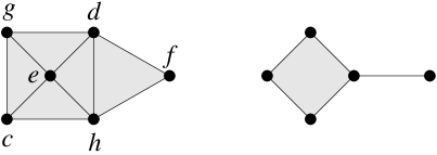
Figure 6: The order complex of $J(Q_{3})$ with $a,b,i,j$ omitted, and the interior face dual complex

We mentioned earlier that in general the coefficients of the mixed lattice point enumerator $N(x_{1}{\cal P}_{1}+\cdots+x_{n}{\cal P}_{n})$ may be negative. The polytope $\Pi_{n}({\mbox{\boldmath$x$}})$ is an exception, however, and in fact satisfies a slightly stronger property.

Corollary 10

The polynomial $N(\Pi_{n}(x_{1}-1,x_{2},\dots,x_{n}))$ has nonnegative coefficients.

Proof.  Immediate from equation (32), since the polynomial $\left(\left({t\atop i}\right)\right)$ has nonnegative coefficients. $\Box$

Note. One can also think of ${\cal C}_{C}(Q_{n},{\mbox{\boldmath$u$}})$ as the “polytope of fractional shapes contained in the shape $(u_{n},u_{n-1},\dots,u_{1})$.” In general, let $\lambda=(\lambda_{1},\dots,\lambda_{n})$ be a partition, i.e., $\lambda_{i}\in\mathbb{N}$ and $\lambda_{1}\geq\cdots\geq\lambda_{n}$, which we also call a shape. We say that a shape $\mu=(\mu_{1},\dots,\mu_{n})$ is contained in $\lambda$ if $\mu_{i}\leq\lambda_{i}$ for all $i$. (This partial ordering on shapes defines Young’s lattice [32, Exer. 3.63]. Additional properties of Young’s lattice may be found in various places in [34].) If we relax the conditions that the $\lambda_{i}$’s are integers but only require them to be real (with $\lambda_{1}\geq\cdots\geq\lambda_{n}\geq 0$), then we can think of $\lambda$ as a “fractional shape.” Thus ${\cal C}_{C}(Q_{n},{\mbox{\boldmath$u$}})$ just consists of the fractional shapes contained in the shape $(u_{n},u_{n-1},\dots,u_{1})$.

5 Connections with parking functions and plane partitions.

There are two additional interpretations of the volume and lattice point enumerator of $\Pi_{n}({\mbox{\boldmath$x$}})$ that we wish to discuss. The first concerns the subject of parking functions, originally defined by Konheim and Weiss [9]. A parking function of length $n$ may be defined as a sequence $(a_{1},\dots,a_{n})$ of positive integers whose increasing rearrangement $b_{1}\leq\cdots\leq b_{n}$ satisfies $b_{i}\leq i$. For the reason for the terminology “parking function,” as well as additional results and references, see [34, Exercise 5.49]. A basic result of Konheim and Weiss is that the number of parking functions of length $n$ is $(n+1)^{n-1}$.

Write $\mathrm{park}(n)$ for the set of all parking functions of length $n$. For ${\mbox{\boldmath$x$}}=(x_{1},\dots,x_{n})\in\mathbb{N}^{n}$ define an $x$-parking function to be a sequence $(a_{1},\dots,a_{n})$ of positive integers whose decreasing rearrangement $b_{1}\leq\cdots\leq b_{n}$ satisfies $b_{i}\leq x_{1}+\cdots+x_{i}$. Thus an ordinary parking function corresponds to the case ${\mbox{\boldmath$x$}}=(1,1,\dots,1)$. Let $P_{n}({\mbox{\boldmath$x$}})$ denote the number of $x$-parking functions. Note that $P_{n}({\mbox{\boldmath$x$}})=0$ if $x_{1}=0$.

Theorem 11

$$P_{n}({\mbox{\boldmath$x$}})=\sum_{(a_{1},\dots,a_{n})\in\mathrm{park}(n)}x_{a_{1}}\cdots x_{a_{n}}=n!V_{n}({\mbox{\boldmath$x$}})$$ (34)

Proof.  Given $(a_{1},\dots,a_{n})\in\mathrm{park}(n)$, replace each $i$ by an integer in the set $\{x_{1}+\cdots+x_{i-1}+1,\dots,x_{1}+\cdots+x_{i}\}$. The number of ways to do this is given by the middle expression in (34), and every $x$-parking function is obtained exactly once in this way. This yields the first equality. The second equality follows from the expansion (2) of $V_{n}({\mbox{\boldmath$x$}})$, since a parking function is obtained by choosing ${\mbox{\boldmath$k$}}\in K_{n}$, forming a sequence with $k_{i}$ $i$’s, and permuting its elements in ${n\choose k_{1},\dots,k_{n}}$ ways. $\Box$

Take $x_{i}=1$ for all $i$ in (34) and apply (7) for $a=b=1$ to recover the result of [9] that the number of parking functions of length $n$ is $(n+1)^{n-1}$. We note that formula (7) can be given a simple combinatorial proof generalizing the proof of Pollak [5, p. 13] for the case of ordinary parking functions; see [33, p. 10] for the case $a=b$. We note that Theorem 11 also gives enumerative interpretations of formulae (8) and (9). Presumably these formulae too could be derived combinatorially in the setting of parking functions, but we will not attempt that here.

An interesting special case of Theorem 11 arises when we take $x_{i}=q^{i-1}$ for some $q>0$. In this case we have

$$n!\,V_{n}(1,q,q^{2},\dots,q^{n-1})=\sum_{(a_{1},\dots,a_{n})\in\mathrm{park}(n)}q^{a_{1}+\cdots+a_{n}-n}.$$

It follows from a result of Kreweras [11] (see also [34, Exer. 5.49(c)]) that also

$$n!\,V_{n}(1,q,q^{2},\dots,q^{n-1})=q^{{n\choose 2}}I_{n}(1/q),$$

where $I_{n}(q)$ is the inversion enumerator of labeled trees.

We can generalize equation (7) by giving a simple product formula for the Ehrhart polynomial $i(\Pi_{n}({\mbox{\boldmath$x$}}),r)$ of $\Pi_{n}({\mbox{\boldmath$x$}})$ in the case ${\mbox{\boldmath$x$}}=(a,b,b,\dots,b)$ (see Theorem 13). First we need to discuss another way to interpret $N(\Pi_{n}({\mbox{\boldmath$x$}}))$.

Let $\lambda=(\lambda_{1},\dots,\lambda_{\ell})$ be a partition, so $\lambda_{i}\in\mathbb{N}$ and $\lambda_{1}\geq\cdots\geq\lambda_{\ell}\geq 0$. A plane partition of shape $\lambda$ and largest part at most $m$ is an array $\pi=\left(\pi_{ij}\right)$ of integers $1\leq\pi_{ij}\leq m$, defined for $1\leq i\leq\ell$ and $1\leq j\leq\lambda_{i}$, which is weakly decreasing in rows and columns. For instance, the plane partitions of shape $(2,1)$ and largest part at most $2$ are given by

$$\begin{array}[]{lclclclcl}11&&21&&22&&21&&22\\[-3.00003pt] 1&&1&&1&&2&&2\end{array},$$

where we only display the positive parts $\pi_{ij}>0$. Basic information on plane partitions may be found in [34, §§7.20–7.22]. If ${\mbox{\boldmath$x$}}=(x_{1},\dots,x_{n})$ $\,\in\mathbb{N}^{n}$ then set

$${\mbox{\boldmath$u$}}=(u_{1},\dots,u_{n})=(x_{1},x_{1}+x_{2},\cdots,x_{1}+\cdots+x_{n})$$

and write $\tilde{{\mbox{\boldmath$u$}}}=(u_{n},\dots,u_{1})$, so that $\tilde{{\mbox{\boldmath$u$}}}$ is a partition.

Theorem 12

Let ${\mbox{\boldmath$x$}}\in\mathbb{N}^{n}$. Then $N(\Pi_{n}({\mbox{\boldmath$x$}}))$ is equal to the number of plane partitions of shape $\tilde{{\mbox{\boldmath$u$}}}$ and largest part at most $2$.

Proof.  If $(y_{1},\dots,y_{n})\in\Pi_{n}({\mbox{\boldmath$x$}})\cap\mathbb{Z}^{n}$, then define the plane partition $\pi$ of shape $u$ to have $y_{1}+\cdots+y_{i}$ 2’s in row $n+1-i$ and the remaining entries equal to 1. This sets up a bijection between the integer points in $\Pi_{n}({\mbox{\boldmath$x$}})$ and the plane partitions of shape $\tilde{{\mbox{\boldmath$u$}}}$ and largest part at most 2. $\Box$

Note. Because of the connection given by Theorem 12 between integer points in $\Pi_{n}({\mbox{\boldmath$x$}})$ and plane partitions, a number of results concerning $\Pi_{n}({\mbox{\boldmath$x$}})$ appear already (sometimes implicitly) in the plane partition literature. In particular, consider the determinantal formula (6) of Steck. Let $j^{\prime}_{i}=j_{i}-i$, $b^{\prime}_{i}=b_{i}-i+1$, and $c^{\prime}_{i}=c_{i}-i-1$. We are then counting sequences $j^{\prime}_{1}\leq j^{\prime}_{2}\leq\cdots\leq j^{\prime}_{n}$ satisfying $b^{\prime}_{i}\leq j^{\prime}_{i}\leq c^{\prime}_{i}$. If $b^{\prime}_{i}>b^{\prime}_{i+1}$ then we can replace $b^{\prime}_{i+1}$ by $b^{\prime}_{i}$ without affecting the sequences $j^{\prime}_{1}\leq\cdots\leq j^{\prime}_{n}$ being counted. Similarly if $c^{\prime}_{i}>c^{\prime}_{i+1}$ we can replace $c^{\prime}_{i}$ with $c^{\prime}_{i+1}$. Moreover, clearly the number of sequences being counted is not changed by adding a fixed integer $k$ to each $b^{\prime}_{i}$ and $c^{\prime}_{i}$. Hence it costs nothing to assume that $0\leq b^{\prime}_{1}\leq\cdots\leq b^{\prime}_{n}$ and $0\leq c^{\prime}_{1}\leq\cdots\leq c^{\prime}_{n}$ (with $b^{\prime}_{i}\leq c^{\prime}_{i}$). Let $\lambda=(c^{\prime}_{n},\dots,c^{\prime}_{1})$ and $\mu=(b^{\prime}_{n},\dots,b^{\prime}_{1})$. Then $\lambda$ and $\mu$ are partitions, and $\mu\subseteq\lambda$ in the sense of containment of diagrams (see [34, §7.2]). Let $Y$ denote the poset (actually a distributive lattice) of all partitions of all nonnegative integers, ordered by diagram containment. The lattice $Y$ is just Young’s lattice mentioned above. In terms of Young’s lattice, we see that that the number $\#(b,c)$ of equation (6) is just the number of elements $(j^{\prime}_{n},\dots,j^{\prime}_{1})$ in the interval $[\mu,\lambda]$ of $Y$. Alternatively, $\#(b,c)$ is the number of multichains $\mu=\lambda^{0}\leq\lambda^{1}\leq\lambda^{2}=\lambda$ of length two in the interval $[\mu,\lambda]$ of $Y$. Kreweras [10, §2.3.7] gives a determinantal formula for the number of multichains of any fixed length $k$ in the interval $[\mu,\lambda]$. (See also [32, Exer. 3.63].) Such a multichain is easily seen to be equivalent to a plane partition of shape $\lambda/\mu$ with largest part at most $k$. When specialized to $k=2$, Kreweras’ formula becomes precisely our equation (25). Moreover, the special case $\mu=\emptyset$ of Kreweras’ formula was already known to MacMahon (put $x=1$ in the implied formula for $GF(p_{1}p_{2}\cdots p_{m};n)$ in [14, p. 243]). By Theorem 12 the number of elements of the interval $[\emptyset,\lambda]$ is just $N(\Pi_{n}({\mbox{\boldmath$x$}}))$, where $\lambda$ is the partition $\tilde{{\mbox{\boldmath$u$}}}$ of Theorem 12. Hence in some sense MacMahon already knew a determinantal formula for $N(\Pi_{n}({\mbox{\boldmath$x$}}))$ and thus also (by taking leading coefficients of $N(\Pi_{n}(r{\mbox{\boldmath$x$}}))$ regarded as a polynomial in $r$) for the volume $V_{n}({\mbox{\boldmath$x$}})$.

Theorem 13

Let $a,b\in\mathbb{N}$ and ${\mbox{\boldmath$x$}}=(a,b,b,\dots,b)\in\mathbb{N}^{n}$. Then the Ehrhart polynomial $i(\Pi_{n}({\mbox{\boldmath$x$}}))$ is given by

$$i(\Pi_{n}({\mbox{\boldmath$x$}}),r)=\frac{1}{n!}(ra+1)(r(a+nb)+2)(r(a+nb)+3)\cdots(r(a+nb)+n).$$ (35)

In particular, the number $N(\Pi_{n}({\mbox{\boldmath$x$}}))$ of integer points in $\Pi_{n}({\mbox{\boldmath$x$}})$ satisfies

$$N(\Pi_{n}({\mbox{\boldmath$x$}}))=\frac{1}{n!}(a+1)(a+nb+2)(a+nb+3)\cdots(a+nb+n).$$

First proof. The theorem is simply a restatement of a standard result in the subject of ballot problems and lattice path enumeration, going back at least to Lyness [13], and with many proofs. A good discussion appears in [19, §§1.4–1.6]. See also [20, §1.3, Lemma 3B].

Second proof. We give a proof different from the proofs alluded to above, because it has the virtue of generalizing to give Theorem 14 below. The polytope $r\Pi_{n}({\mbox{\boldmath$x$}})$ is just $\Pi_{n}(r{\mbox{\boldmath$x$}})$. Hence by Theorem 12 $i(\Pi_{n}({\mbox{\boldmath$x$}}),r)$ is just the number of plane partitions of shape $r{\mbox{\boldmath$u$}}$ and largest part at most 2. Identify the partition $u$ with its diagram, consisting of all pairs $(i,j)$ with $1\leq i\leq n$ and $1\leq j\leq\tilde{u}_{i}=a+(n-i)b$. Define the content $c(s)$ of $s=(i,j)\in\tilde{{\mbox{\boldmath$u$}}}$ by $c(s)=j-i$ (see [34, p. 373]). An explicit formula for the number of plane partitions of shape $u$ and any bound on the largest part was first obtained by Proctor and is discussed in [34, Exer. 7.101] (as well as a generalization due to Krattenthaler). Proctor’s formula for the case at hand gives

$$i(\Pi_{n}({\mbox{\boldmath$x$}}),r)=\prod_{{s=(i,j)\in r\tilde{{{{\mbox{${\mbox{\tiny\boldmath$u$}}$}}}}}\atop n+c(s)\leq r\tilde{u}_{i}}}\frac{1+n+c(s)}{n+c(s)}\ \prod_{{s=(i,j)\in r\tilde{{{{\mbox{${\mbox{\tiny\boldmath$u$}}$}}}}}\atop n+c(s)>r\tilde{u}_{i}}}\frac{rb+1+n+c(s)}{n+c(s)}.$$

When all the factors of the above products are written out, there is considerable cancellation. The only denominator factors that survive are those indexed by $(i,1)$, $1\leq i\leq n$, yielding the denominator $n!$. The surviving numerator factors are $ra+1$ (indexed by $(n,ra)$) and $r(a+nb)+k$, $2\leq k\leq n$ (indexed by $(1,r(a+(n-1)b)-n+k)$), the last $n-1$ squares in the first row of $\tilde{{\mbox{\boldmath$u$}}}$). $\Box$

Note from (35) that the leading coefficient of $i(\Pi_{n}({\mbox{\boldmath$x$}}),r)$ (and hence the volume $V_{n}({\mbox{\boldmath$x$}})$ of $\Pi_{n}({\mbox{\boldmath$x$}})$) is given by $a(a+nb)^{n-1}$, agreeing with equation (7).

There is a straightforward generalization of Theorems 12 and 13 involving plane partitions of shape $u$ with largest part at most $m+1$ (instead of just $m+1=2$). Given ${\mbox{\boldmath$x$}}\in\mathbb{N}^{n}$ as before, let $\Pi_{n}^{m}({\mbox{\boldmath$x$}})\subset\mathbb{R}^{nm}$ be the polytope of all $n\times m$ matrices $\left(y_{ij}\right)$ satisfying $y_{ij}\geq 0$ and

$$v_{i1}\leq v_{i2}\leq\cdots\leq v_{im}\leq x_{1}+\cdots+x_{i},$$

for $1\leq i\leq n$, where

$$v_{ij}=y_{i1}+y_{i2}+\cdots+y_{ij}.$$

Thus $\Pi_{n}^{1}({\mbox{\boldmath$x$}})=\Pi_{n}({\mbox{\boldmath$x$}})$. Then the proof of Theorem 12 carries over mutatis mutandis to show that $N(\Pi_{n}^{m}({\mbox{\boldmath$x$}}))$ is the number of plane partitions of shape $\tilde{{\mbox{\boldmath$u$}}}$ and largest part at most $m+1$. The result of Proctor mentioned above gives an explicit formula for this number when ${\mbox{\boldmath$x$}}=(a,b,b,\dots,b)$. Replacing $x$ by $r{\mbox{\boldmath$x$}}$ and computing the leading coefficient of the resulting polynomial in $r$ gives a formula for the volume $V_{n}^{m}({\mbox{\boldmath$x$}})$ of $\Pi_{n}^{m}({\mbox{\boldmath$x$}})$. This computation is similar to that in the proof of Theorem 13, though the details are more complicated. We merely state the result here without proof. Is there a direct combinatorial proof similar to the proofs of Theorem 13 (the case $m=1$ of Theorem 14) appearing in [19] and [20]?

Theorem 14

Let ${\mbox{\boldmath$x$}}=(a,b,b,\dots,b)\in\mathbb{N}^{n}$. Then

$$(nm)!\,V_{n}^{m}({\mbox{\boldmath$x$}})=1!\,2!\,\cdots m!\,f^{\langle m^{n}\rangle}(n+m)^{n-1}(n+m-1)^{n-2}\cdots(n+1)^{n-m},$$

where $f^{\langle m^{n}\rangle}$ denotes the number of standard Young tableaux of shape $\langle m^{n}\rangle=$ $(m,m,\dots,m)$ ($n$ $m$’s in all), given explicitly by the “hook-length formula” [34, Cor. 7.21.6].

There is a further generalization of the polytope $\Pi_{n}({\mbox{\boldmath$x$}})$ which deserves mention. Let ${\mbox{\boldmath$x$}}=(x_{1},\dots,x_{n})\in\mathbb{R}_{\geq 0}^{n}$ and ${\mbox{\boldmath$z$}}=(z_{1},\dots,z_{n})\in\mathbb{R}_{\geq 0}^{n}$, with $v_{i}=z_{1}+\cdots+z_{i}\leq x_{1}+\cdots+x_{i}=u_{i}$. Let $\Pi_{n}({\mbox{\boldmath$z$}},{\mbox{\boldmath$x$}})$ be the polytope of all points $(y_{1},\dots,y_{n})\in\mathbb{R}^{n}$ satisfying

$$y_{i}\geq 0,\ \mbox{for}\ 1\leq i\leq n$$

$$v_{i}\leq y_{1}+\cdots+y_{i}\leq u_{i}.$$

Thus $\Pi_{n}({\mbox{\boldmath$x$}})=\Pi_{n}({\mbox{\boldmath$0$}},{\mbox{\boldmath$x$}})$. Much of the theory of $\Pi_{n}({\mbox{\boldmath$x$}})$ extends to $\Pi_{n}({\mbox{\boldmath$z$}},{\mbox{\boldmath$x$}})$. Rather than enter into the details here, we simply illustrate with the case $n=2$ how the polyhedral decomposition of $\Pi_{n}({\mbox{\boldmath$x$}})$ with chambers $\Lambda_{\pi}$ extends to $\Pi_{n}({\mbox{\boldmath$z$}},{\mbox{\boldmath$x$}})$. In general, the chambers $\Lambda_{\pi}$ of a decomposition of $\Pi_{n}({\mbox{\boldmath$z$}},{\mbox{\boldmath$x$}})$ into a product of simplices will be obtained from linear extensions $\pi=a_{1}a_{2}\cdots a_{3n}$ of ${\mbox{\boldmath$3$}}\times{\mbox{\boldmath$n$}}$. Let the elements of ${\mbox{\boldmath$3$}}\times{\mbox{\boldmath$n$}}$ be $\alpha_{1},\dots,\alpha_{3n}$ with $\alpha_{1}<\cdots<\alpha_{n}$, $\alpha_{n+1}<\cdots<\alpha_{2n}$, $\alpha_{2n+1}<\cdots<\alpha_{3n}$, and $\alpha_{i}<\alpha_{n+i}<\alpha_{2n+i}$ for $1\leq i\leq n$. Then $\pi$ corresponds to the chamber

$$0\leq f(\alpha_{1})\leq\cdots\leq f(\alpha_{3n}),$$ (36)

where

$$f(\alpha_{i})=\left\{\begin{array}[]{rl}v_{i},&\mbox{if}\ 1\leq i\leq n\\ y_{1}+\cdots+y_{i-n},&\mbox{if}\ n+1\leq i\leq 2n\\ u_{i-2n},&\mbox{if}\ 2n+1\leq i\leq 3n.\end{array}\right.$$

There is one important difference between this decomposition and the analogous one for $\Pi_{n}({\mbox{\boldmath$x$}})$, namely, in the present case some of the chambers $\Lambda_{\pi}$ will actually be empty and should be ignored. (Of course $\Lambda_{\pi}$ isn’t really a chamber if it’s empty.) The question of which are empty will depend on the relative order of the numbers $u_{1},\dots,u_{n}$ and $v_{1},\dots,v_{n}$. In the “generic” case when each $x_{i}>0$ and $z_{i}>0$ there are $C_{n}$ (a Catalan number) relative orderings of the $u_{i}$’s and $v_{i}$’s (since $u_{1}<\cdots<u_{n}$, $v_{1}<\cdots<v_{n}$, and $v_{i}\leq u_{i}$). More generally, we can change some of the $\leq$ signs in equation (36) to $<$ signs, in accordance with the descents of the corresponding linear extension $\pi$, so that we obtain a decomposition of $\Pi_{n}({\mbox{\boldmath$z$}},{\mbox{\boldmath$x$}})$ into pairwise disjoint cells from which we can compute the lattice point enumerator $N(\Pi_{n}({\mbox{\boldmath$z$}},{\mbox{\boldmath$x$}}))$.

Let us illustrate the above discussion in the case $n=2$. The linear extensions of ${\mbox{\boldmath$3$}}\times{\mbox{\boldmath$2$}}$, using the labeling just described, are given by

$$\begin{array}[]{l}1\,2\,3\,4\,5\,6\\ 1\,2\,3\,5\,4\,6\\ 1\,3\,2\,4\,5\,6\\ 1\,3\,2\,5\,4\,6\\ 1\,3\,5\,2\,4\,6\end{array}.$$

Thus the following sets (possibly empty) give a decomposition of $\Pi_{n}({\mbox{\boldmath$z$}},{\mbox{\boldmath$x$}})$ into pairwise disjoint cells:

$$\begin{array}[]{l}0\leq v_{1}\leq v_{2}\leq y_{1}\leq y_{1}+y_{2}\leq u_{1}\leq u_{2}\\ 0\leq v_{1}\leq v_{2}\leq y_{1}\leq u_{1}<y_{1}+y_{2}\leq u_{2}\\ 0\leq v_{1}\leq y_{1}<v_{2}\leq y_{1}+y_{2}\leq u_{1}\leq u_{2}\\ 0\leq v_{1}\leq y_{1}<v_{2}\leq u_{1}<y_{1}+y_{2}\leq u_{2}\\ 0\leq v_{1}\leq y_{1}\leq u_{1}<v_{2}\leq y_{1}+y_{2}\leq u_{2}.\end{array}$$

The first four cells are nonempty provided $v_{2}\leq u_{1}$, while the last cell is nonempty provided $v_{2}>u_{1}$. Hence we read off that

$$N(\Pi_{n}({\mbox{\boldmath$z$}},{\mbox{\boldmath$x$}}))=\left\{\begin{array}[]{rl}A,&x_{1}\geq z_{1}+z_{2}\\ \left(\left({x_{1}-z_{1}+1\atop 1}\right)\right)\left(\left({x_{1}+x_{2}-z_{1}-z_{2}+1\atop 1}\right)\right),&x_{1}<z_{1}+z_{2},\end{array}\right.$$

where

$$A=\left({x_{1}-z_{1}-z_{2}+1\choose 2}\right)+\left({x_{1}-z_{1}-z_{2}+1\choose 1}\right)\left({x_{2}\choose 1}\right)$$

$$\qquad+\left({z_{2}\choose 1}\right)\left({x_{1}-z_{1}-z_{2}+1\choose 1}\right)+\left({z_{2}\choose 1}\right)\left({x_{2}\choose 1}\right).$$

6 A subdivision of $\Pi_{n}({\mbox{\boldmath$x$}})$ connected with the associahedron

In this section we describe a polyhedral subdivison $(\hat{\Pi}_{n}({\mbox{\boldmath$k$}};{\mbox{\boldmath$x$}}),\ {\mbox{\boldmath$k$}}\in K_{n})$ of $\Pi_{n}({\mbox{\boldmath$x$}})$ different from the subdivision discussed in Section 3. This subdivision is closely related to a convex polytope known as the associahedron, defined as follows. Let $E_{n+2}$ be a convex $(n+2)$-gon. A polygonal decomposition of $E_{n+2}$ consists of a set of diagonals of $E_{n+2}$ that do not cross in their interiors. Hence the maximal polygonal decompositions are the triangulations, and contain exactly $n-1$ diagonals. Let $\mathrm{dec}(E_{n+2})$ denote the poset of all polygonal decompositions of $E_{n+2}$, ordered by inclusion, with a top element $\hat{1}$ adjoined. It was first shown by C. W. Lee [12] and M. Haiman [7] that $\mathrm{dec}(E_{n+2})$ is the face lattice of an $(n-1)$-dimensional convex polytope ${\cal A}_{n}$, known as the associahedron or Stasheff polytope. (Earlier Stasheff [35] defined the dual of the associahedron as a simplicial complex and constructed a geometric realization as a convex body but not as a polytope.) A vast generalization is discussed in [6, Ch. 7]. For some further information see [34, Exer. 6.33].

We next give a somewhat different description of the associahedron (or more precisely, of its face lattice) that is most convenient for our purposes. A fan in $\mathbb{R}^{m}$ is a (finite) collection $F$ of pointed polyhedral cones (with vertices at the origin) satisfying the two conditions:

• If ${\cal C},{\cal C}^{\prime}\in{\mbox{\boldmath$F$}}$ then ${\cal C}\cap{\cal C}^{\prime}$ is a face (possibly consisting of just the origin) of ${\cal C}$ and ${\cal C}^{\prime}$.

• If ${\cal C}\in{\mbox{\boldmath$F$}}$ and ${\cal C}^{\prime}$ is a face of ${\cal C}$, then ${\cal C}^{\prime}\in{\mbox{\boldmath$F$}}$.

A fan $F$ is called complete if $\bigcup_{{\cal C}\in{{{\mbox{${\mbox{\scriptsize\boldmath$F$}}$}}}}}=\mathbb{R}^{m}$.

We will define a fan whose chambers are indexed by plane binary trees with $n$ internal vertices. The definition of a plane tree may be found for instance in [32, Appendix]. The key point is that the subtrees of any vertex are linearly ordered $T_{1},\dots,T_{k}$, indicated in drawing the tree (with the root on the bottom) by placing the subtrees in the order $T_{1},\dots,T_{k}$ from left to right. A binary plane tree is a plane tree for which each vertex $v$ has zero or two subtrees. In the latter case we call the vertex an internal vertex. Otherwise $v$ is a leaf or endpoint. We will always regard plane trees as being drawn with the root at the bottom.

Let $T$ be a plane binary tree with $n$ internal vertices (so $n+1$ leaves). The number of such trees is the Catalan number $C_{n}$ [34, 6.19(d)]. Do a depth-first search through $T$ (as defined e.g. in [34, pp. 33–34]) and label the internal vertices $1,2,\dots,n$ in the order they are first encountered from above. Equivalently, every internal vertex is greater than those in its left subtree, and smaller than those in its right subtree. We call this labeling of the internal vertices of $T$ the binary search labeling. Figure 7 gives an example when $n=4$. Let $y_{1},\dots,y_{n-1}$ denote the coordinates in $\mathbb{R}^{n-1}$. If the internal vertex $i$ of $T$ (using the labeling just defined) is covered by $j$ and $i<j$, then associate with the pair $(i,j)$ the inequality

$$y_{i+1}+y_{i+2}+\cdots+y_{j}\leq 0,$$ (37)

while if $i>j$ then associate with $(i,j)$ the inequality

$$y_{j+1}+y_{j+2}+\cdots+y_{i}\geq 0.$$ (38)

We get a system of $n-1$ homogeneous linear inequalities that define a simplicial cone ${\cal C}_{T}$ in $\mathbb{R}^{n-1}$. For example, the inequalities corresponding to the tree of Figure 7 are given by

$$y_{2} \leq 0$$

$$y_{2}+y_{3} \geq 0$$

$$y_{4} \geq 0.$$

Figure 7: A plane tree with the binary search labeling of its internal vertices

It is not hard to check that these $C_{n}$ cones, as $T$ ranges over all plane binary trees with $n$ internal vertices, form the chambers of a complete fan ${\mbox{\boldmath$F$}}\!_{n}$ in $\mathbb{R}^{n-1}$. For instance, Figure 8 shows the fan ${\mbox{\boldmath$F$}}\!_{3}$.

Figure 8: The fan ${\mbox{\boldmath$F$}}\!_{3}$

Theorem 15

The face poset $P({\mbox{\boldmath$F$}}\!_{n})$ of the fan ${\mbox{\boldmath$F$}}\!_{n}$, with a top element $\hat{1}$ adjoined, is isomorphic to the dual $\mathrm{dec}(E_{n+2})^{*}$ of the face lattice of the associahedron ${\cal A}_{n+2}$.

Proof.  The face lattice of a complete fan is completely determined by the incidences between the chambers and extreme rays. (See [32, Exer. 3.12] for a stronger statement.) The chambers of ${\mbox{\boldmath$F$}}\!_{n}$ have already been described in terms of plane binary trees. There is a well-known bijection between plane binary trees on $2n+1$ vertices and triangulations of a convex $(n+2)$-gon $E_{n+2}$. This bijection is explained for instance in [34, Cor. 6.2.3]. In particular, to define the bijection we first need to fix an edge $\varepsilon$ of $E_{n+2}$, called the root edge. We hope that Figure 9 will make this bijection clear; see the previous reference for further details. Thus we have a bijection between the chambers ${\cal C}$ of ${\mbox{\boldmath$F$}}\!_{n}$ and the triangulations of the convex $(n+2)$-gon $E_{n+2}$.

We now describe the extreme rays $R$ of ${\mbox{\boldmath$F$}}\!_{n}$. We can describe $R$ uniquely by specifying one nonzero point on $R$. We will index these points by the diagonals $D$ of a convex $(n+2)$-gon $E_{n+2}$. Label the vertices of $E_{n+2}$ as $0,1,\dots,n+1$ clockwise beginning with one vertex of $\varepsilon$ and ending with the other. Let $e_{i}$ denote the unit coordinate vector corresponding to the coordinate $y_{i}$ in the space $\mathbb{R}^{n-1}$ with coordinates $y_{2},\dots,y_{n}$. Given the diagonal $D$ between vertices $i<j$ of $E_{n+2}$, associate a point $p_{D}\in\mathbb{R}^{n-1}$ as follows:

$$p_{D}=\left\{\begin{array}[]{rl}e_{j},&\mbox{if}\ i=0\\ -e_{i+1},&\mbox{if}\ j=n+1\\ e_{j}-e_{i+1},&\mbox{otherwise}.\end{array}\right.$$

We claim that the ray $\{\alpha p_{D}\,:\,\alpha\in\mathbb{R}_{\geq 0}\}$ is the extreme ray of ${\mbox{\boldmath$F$}}\!_{n}$ that is the intersection of all the chambers of ${\mbox{\boldmath$F$}}\!_{n}$ corresponding to the triangulations of $E_{n+2}$ that contain $D$. From this claim the proof of the theorem follows (using the fact that ${\mbox{\boldmath$F$}}\!_{n}$ is a simplicial fan, i.e., every face is a simplicial cone).

Consider first the diagonal $D$ with vertices 0 and $j$. Let $\Upsilon$ be a triangulation of $E_{n+2}$ containing $D$. The internal vertices of $T$ corresponding to the regions (triangles) of the triangulation $\Upsilon$. Because of our procedure for labeling the internal vertices of a plane binary tree $T$, it follows that the labels of the internal vertices “above” $D$ (i.e., on the opposite side of $D$ as the root edge $\varepsilon$) will be $1,2,\dots,j-1$, while the internal vertices below $D$ will be labeled $j,j+1,\dots,n$. (See Figure 9 for an example with $n=8$. The diagonal $D$ in question is labeled $D_{1}$ and connects vertex 0 to vertex $j=6$. The plane binary tree $T$ is drawn with dashed lines.) Consider the internal edges of $T$ that give rise (via equations (37) and (38)) to chambers whose equations involve $y_{j}$. No such edge can appear below $D$, since $j$ is the least vertex label appearing below $D$. Similarly no such edge can appear above $D$, since only vertices less than $j$ appear above $D$. Hence such an edge must cross $D$. The top (farthest from the root) vertex $a$ of this edge is $<j$, while the bottom vertex $b$ is $\geq j$. Hence the chamber equation is given by $y_{a+1}+y_{a+2}+\cdots+y_{b}\geq 0$, where $a<j$ and $b\geq j$. Hence the point $e_{j}$ lies on this chamber, and so the ray through $e_{j}$ is the intersection of the chambers corresponding to triangulations containing $D$.

Figure 9: A triangulated 10-gon and the corresponding plane binary tree $T$

A completely analogous argument holds for the diagonal $D$ with vertices $i$ and $n+1$.

Finally suppose that $D$ has vertices $i,j$ where $0<i<j<n+1$. The internal vertices of $T$ appearing above $D$ will be labeled $i+1,i+2,\dots,j-1$, while the remaining vertex labels appear below $D$. (See Figure 9, where the diagonal $D$ in question is labeled $D_{2}$, and where $i=2$ and $j=6$.) Consider an internal edge of $T$ whose vertex labels are $a$ and $b$ where $a\leq i$ and $i+1\leq b<j$. These are precisely the edges whose corresponding chamber equation (either $y_{a+1}+y_{a+2}+\cdots+y_{b}\geq 0$ or $y_{a+1}+y_{a+2}+\cdots+y_{b}\leq 0$) involves $y_{i+1}$ but not $y_{j}$. Since $b$ appears above $D$ and $a$ below, the chamber equation is in fact $y_{a+1}+y_{a+2}+\cdots+y_{b}\leq 0$. In particular, the point $e_{j}-e_{i+1}$ lies on the chamber. Similarly, consider an internal edge of $T$ whose labels are $a$ and $b$ where $i+1\leq a<j$ and $j\leq b$. These are precisely the edges whose corresponding chamber equation (again either $y_{a+1}+y_{a+2}+\cdots+y_{b}\geq 0$ or $y_{a+1}+y_{a+2}+\cdots+y_{b}\leq 0$) involves $y_{j}$ but not $y_{i+1}$. Since $b$ appears below $D$ and $a$ above, the chamber equation is in fact $y_{a+1}+y_{a+2}+\cdots+y_{b}\geq 0$. In particular, the point $e_{j}-e_{i+1}$ lies on the chamber. Every other chamber equation either involves neither $y_{i+1}$ nor $y_{j}$, or else involves both (with a coefficient 1). Hence $e_{i+1}-e_{j}$ lies on every chamber corresponding to a triangulation containing $D$, so the intersection of these chambers is the ray containing $e_{j}-e_{i+1}$. This completes the proof of the claim, and with it the theorem. $\Box$

The connection between $\Pi_{n}({\mbox{\boldmath$x$}})$ and the fan ${\mbox{\boldmath$F$}}\!_{n}$ is provided by the concept of a plane tree with edge lengths. If we associate with each edge $e$ of the plane tree $T$ a positive real number $\ell(e)$, then we call the pair $(T,\ell)$ a plane tree with edge lengths. Such a tree can be drawn by letting the length of each edge $e$ be $\ell(e)$.

Now fix a real number $s>0$, which will be the sum of the edge lengths of a plane tree. Let ${\mbox{\boldmath$x$}}=(x_{1},\dots,x_{n})\in\mathbb{R}_{+}^{n}$ with $\sum x_{i}<s$. Let ${\mbox{\boldmath$y$}}=(y_{1},\dots,y_{n})\in\mathbb{R}_{+}^{n}$ with $y_{1}+\cdots+y_{i}\leq x_{1}+\cdots+x_{i}$ for $1\leq i\leq n$. We associate with the pair $({\mbox{\boldmath$x$}},{\mbox{\boldmath$y$}})$ a plane tree with edge lengths $\varphi({\mbox{\boldmath$x$}},{\mbox{\boldmath$y$}})=(\bar{T},\ell)$ as follows. Start at the root and traverse the tree in preorder (or depth-first order) [34, pp. 33–34]. First go up a distance $x_{1}$, then down a distance $y_{1}$, then up a distance $x_{2}$, then down a distance $y_{2}$, etc. After going down a distance $y_{n}$, complete the tree by going up a distance $x_{n+1}=s-x_{1}-\cdots-x_{n}$ and then down a distance $y_{n+1}=s-y_{1}-\cdots-y_{n}$. Generically we obtain a planted plane binary tree with edge lengths, i.e, the root has degree one (or one child), and all other internal vertices have degree two. Figure 10 shows the planted plane binary tree with edge lengths associated with $s=16$ and ${\mbox{\boldmath$x$}}=(6,2,7)$, ${\mbox{\boldmath$y$}}=(1,4,3)$. If $\bar{T}$ is a planted plane tree, then we let $T$ denote the tree obtained by “unplanting” (uprooting?) $\bar{T}$, i.e., remove from $\bar{T}$ the root and its unique incident edge $e$ (letting the other vertex of $e$ become the root of $T$).

Figure 10: A planted plane binary tree with edge lengths

Fix the sequence ${\mbox{\boldmath$x$}}=(x_{1},\dots,x_{n})$ with $\sum x_{i}<s$. For a plane binary tree $T$ (without edge lengths) with $n$ internal vertices (and hence $n+1$ leaves), define $\Delta_{T}=\Delta_{T}({\mbox{\boldmath$x$}})$ to be the set of all ${\mbox{\boldmath$y$}}=(y_{1},\dots,y_{n})\in\mathbb{R}_{+}^{n}$ such that $\varphi({\mbox{\boldmath$x$}},{\mbox{\boldmath$y$}})=(\bar{T},\ell)$ for some $\ell$. Let ${\cal T}_{n}$ denote the set of plane binary trees with $n$ internal vertices. Let $T\in{\cal T}_{n}$ with the binary search labeling of its internal vertices as defined earlier in this section. We now define a sequence ${\mbox{\boldmath$k$}}(T)=(k_{1},\dots,k_{n})\in\mathbb{N}^{n}$ as follows: (1) $k_{i}=0$ if the left child of vertex $i$ is an internal vertex. (2) If the left child of vertex $i$ is an endpoint, then let $k_{i}$ be the largest integer $r$ for which there is a chain $i=j_{1}<j_{2}<\cdots<j_{r}$ of internal vertices such that $j_{h}$ is a left child of $j_{h+1}$ for $1\leq h\leq r-1$. For instance, if $T$ is the tree of Figure 11 then ${\mbox{\boldmath$k$}}(T)=(2,3,0,1,0,1,0,2,0)$.

Figure 11: A plane binary tree $T$ with ${\mbox{\boldmath$k$}}(T)=(2,3,0,1,0,1,0,2,0)$

Lemma 16

The map $T\mapsto{\mbox{\boldmath$k$}}(T)$ is a bijection from ${\cal T}_{n}$ to the set $K_{n}$ defined by equation (3).

Proof.  Let ${\mbox{\boldmath$k$}}(T)=(k_{1},\dots,k_{n})$. The chains $i=j_{1}<j_{2}<\cdots<j_{r}$ described above partition the internal vertices of $T$, so $\sum k_{i}=n$. Since $k_{j_{2}}=\cdots=k_{j_{r}}=0$, it follows that $k_{h+1}+k_{h+2}+\cdots+k_{n}\leq n-h$ for $0\leq h\leq n-1$. Hence $k_{1}+\cdots+k_{h}\geq h$, so ${\mbox{\boldmath$k$}}(T)\in K_{n}$.

It remains to show that given ${\mbox{\boldmath$k$}}=(k_{1},\dots,k_{n})\in K_{n}$, there is a unique $T\in{\cal T}_{n}$ such that ${\mbox{\boldmath$k$}}(T)={\mbox{\boldmath$k$}}$. We can construct the subtree of internal vertices of $T$ as follows. Let $T_{1}$ be defined by starting at the root and making $k_{1}-1$ steps to the left. (Each step is from a vertex to an adjacent vertex.) Hence we have $k_{1}$ vertices in all, and we are located at the vertex furthest from the root. Suppose that $T_{i}$ has been constructed for $i<n$, and that we are located at vertex $v_{i}$. If $k_{i+1}>0$, then move one step to the right and $k_{i+1}-1$ steps to the left, yielding the tree $T_{i+1}$ and the vertex $v_{i+1}$ at which we are located. If $k_{i+1}=0$, then move down the tree (toward the root) until we have traversed exactly one edge in a southeast direction. This gives the tree $T_{i+1}=T_{i}$ and a new present location $v_{i+1}$. Let $T=T_{n}$. It is easily checked that the definition of $K_{n}$ ensures that $T$ is defined (and, though not really needed here, that $v_{n}$ is the root vertex) and ${\mbox{\boldmath$k$}}(T)={\mbox{\boldmath$k$}}$. Since there are $C_{n}=\frac{1}{n+1}{2n\choose n}$ plane binary trees with $n$ internal vertices and since $\#K_{n}=C_{n}$, it follows that the map $T\mapsto{\mbox{\boldmath$k$}}(T)$ is a bijection as claimed. (It is also easy to see directly that $T$ is unique, i.e., if ${\mbox{\boldmath$k$}}(T)={\mbox{\boldmath$k$}}(T^{\prime})$ then $T=T^{\prime}$.) $\Box$

Now given $t\in\mathbb{R}_{+}$, let $\sigma_{k}(t)$ denote the $k$-dimensional simplex of points $(t_{1},\dots,t_{k})$ satisfying $0\leq t_{1}\leq t_{2}\leq\cdots\leq t_{k}\leq t$. Thus

$$\mathrm{Vol}(\sigma_{k}(t))=\frac{t^{k}}{k!}.$$

By convention $\sigma_{0}(t)$ is just a point, with Vol$(\sigma_{0}(t))=1$. We can now state the main result of this section.

Theorem 17

(a) The sets $\Delta_{T}({\mbox{\boldmath$x$}})$, for $T\in{\cal T}_{n}$, form the maximal faces (chambers) of a polyhedral decomposition $\Gamma_{n}$ of $\Pi_{n}({\mbox{\boldmath$x$}})$.

(b) Let ${\mbox{\boldmath$k$}}(T)=(k_{1},\dots,k_{n})$, where $T\in{\cal T}_{n}$. Then $\Delta_{T}({\mbox{\boldmath$x$}})$ is integrally equivalent (as defined at the beginning of Section 4) to the product $\sigma_{k_{1}}(x_{1})\times\cdots\times\sigma_{k_{n}}(x_{n})$, so in particular

$$\mathrm{Vol}(\Delta_{T}({\mbox{\boldmath$x$}}))=\frac{x_{1}^{k_{1}}}{k_{1}!}\cdots\frac{x_{n}^{k_{n}}}{k_{n}!}.$$

(c) The interior face complex $\Gamma_{n}^{\circ}$ of $\Gamma_{n}$ is combinatorially equivalent to the dual associahedron, i.e., the set of interior faces of $\Gamma_{n}$, ordered by inclusion, in isomorphic to the face lattice of the dual associahedron.

Proof of (a). The construction of the plane tree with edge lengths $\varphi({\mbox{\boldmath$x$}},{\mbox{\boldmath$y$}})=(\bar{T},\ell)$ is defined if and only if ${\mbox{\boldmath$y$}}\in\Pi_{n}({\mbox{\boldmath$x$}})$. Since generically $\varphi({\mbox{\boldmath$x$}},{\mbox{\boldmath$y$}})$ is a planted plane binary tree, it follows that the sets $\Delta_{T}({\mbox{\boldmath$x$}})$, $T\in{\cal T}_{n}$, form the chambers of a polyhedral decomposition of $\Pi_{n}({\mbox{\boldmath$x$}})$. $\Box$

Proof of (b). Let $\varphi({\mbox{\boldmath$x$}},{\mbox{\boldmath$y$}})=(\bar{T},\ell)$ as above. Call a vertex $v$ of $\bar{T}$ a left leaf if it is a leaf (endpoint) and is the left child of its parent. Similarly a right edge is an edge that slants to the right as we move away from the root. Let $P(v)$ be the path from the left leaf $v$ toward the root that terminates after the first right edge is traversed (or terminates at the root if there is no such right edge). Let $c(v)$ be the label of the (internal) vertex covered by $v$. Then the length of the path $P(v)$ is just $x_{c(v)}$. If $c(v)=i$, then exactly $k_{i}$ of the paths $P(u)$ end at the path $P(v)$. Suppose that these paths are $P(u_{1}),\dots,P(u_{k_{i}})$ where $u_{1}<\cdots<u_{k_{i}}$. Then the paths $P(u_{j})$ intersect the path $P(v)$ in the order $P(u_{1}),\dots,P(u_{k_{i}})$ from the bottom up. Hence for each $i$ with $k_{i}>0$, we can independently place on a path of length $x_{i}$ the $k_{i}$ points that form the bottoms of the paths $P(u_{j})$. The placement of these points defines a point in a simplex integrally equivalent to $\sigma_{k_{i}}(x_{i})$, so $\Delta_{T}({\mbox{\boldmath$x$}})$ is integrally equivalent to $\sigma_{k_{1}}(x_{1})\times\cdots\times\sigma_{k_{n}}(x_{n})$ as claimed. $\Box$

Example 18

Let $\bar{T}$ be the planted plane binary tree of Figure 12. On the path of length $x_{1}$ from the root $r$ to $v_{1}$ we can place vertices $1$ and $3$ in bijection with the points of the simplex $0\leq t_{3}\leq t_{1}\leq x_{1}$ of volume $x_{1}^{2}/2$. On the path of length $x_{2}$ from 1 to $v_{2}$ we can place vertex $2$ in bijection with the points of the simplex $0\leq t_{2}\leq x_{2}$, of volume $x_{2}$. Finally on the path of length $x_{4}$ from $3$ to $v_{3}$ we can place vertices $4,5,6$ in bijection with the points of the simplex $0\leq t_{6}\leq t_{5}\leq t_{4}\leq x_{4}$, of volume $x_{4}^{3}/6$. Hence $\Delta_{T}$ is integrally equivalent to the product $\sigma_{2}(x_{1})\times\sigma_{1}(x_{2})\times\sigma_{3}(x_{4})$, of volume $x_{1}^{2}x_{2}x_{4}^{3}/2!\,1!\,3!$.

Figure 12: A planted plane binary tree

It is easy to make the integral equivalence between $\Delta_{T}$ and $\sigma_{k_{1}}(x_{1})\times\cdots\times\sigma_{k_{n}}(x_{n})$ completely explicit. For instance, in the above example $t_{3}$ is the distance between vertices $r$ and 3, so

$$t_{3}=x_{1}-y_{1}+x_{2}-y_{2}+x_{3}-y_{3}.$$

Similarly,

$$t_{1}=x_{1}-y_{1}.$$

Now $t_{2}$ is the distance between vertices 1 and 2, so

$$t_{2}=x_{2}-y_{2}.$$

In the same way we obtain

$$t_{6} = x_{4}-y_{y}+x_{5}-y_{5}+x_{6}-y_{6}$$

$$t_{5} = x_{4}-y_{4}+x_{5}-y_{5}$$

$$t_{4} = x_{4}-y_{4}.$$

Proof of (c). Let $\varphi({\mbox{\boldmath$x$}},{\mbox{\boldmath$y$}})=(\bar{T},\ell)$. Then the height (or distance from the root) of vertex $i$ is just $x_{1}+\cdots+x_{i}-y_{1}-\cdots-y_{i}=u_{i}-v_{i}$. Hence if vertex $i$ is covered by $j$ then $u_{i}-v_{i}<u_{j}-v_{j}$. If $i<j$ we get the equation

$$(y_{i+1}-x_{i+1})+\cdots+(y_{j}-x_{j})\leq 0,$$ (39)

while if $i>j$ we get

$$(y_{j+1}-x_{j+1})+\cdots+(y_{i}-x_{i})\geq 0.$$ (40)

Thus these equations, together with $y_{i}\geq 0$ and $y_{1}+\cdots+y_{i}\leq x_{1}+\cdots+x_{i}$, determine $\bar{\Delta}_{T}$.

Note that if we replace each $y_{k}$ by $y_{k}-x_{k}$ in the inequalities (37) and (38) defining the chambers of the fan ${\mbox{\boldmath$F$}}\!_{n}$ of Theorem 15, then we obtain precisely the inequalities (39) and (40). From this we conclude the following. Given ${\mbox{\boldmath$x$}}=(x_{1},\dots,x_{n})\in\mathbb{R}_{\geq 0}^{n}$, translate the fan ${\mbox{\boldmath$F$}}\!_{n}$ so that the center of the translated fan $\widetilde{{\mbox{\boldmath$F$}}}\!_{n}$ is at $(x_{2},\dots,x_{n})$. Add a new $y_{1}$ axis and lift $\widetilde{{\mbox{\boldmath$F$}}}\!_{n}$ into $\mathbb{R}^{n}$, giving a “nonpointed fan” (i.e., a decomposition of $\mathbb{R}^{n}$ satisfying the definition of a fan except that the cones are nonpointed) which we denote by $\widetilde{{\mbox{\boldmath$F$}}}\!_{n}\times\mathbb{R}$. (Thus each cone ${\cal C}\in\widetilde{{\mbox{\boldmath$F$}}}\!_{n}$ lifts to the nonpointed cone ${\cal C}\times\mathbb{R}$.) Finally intersect each chamber (maximal cone) ${\cal C}\times\mathbb{R}$ of $\widetilde{{\mbox{\boldmath$F$}}}\!_{n}\times\mathbb{R}$ with the polytope $\Pi_{n}({\mbox{\boldmath$x$}})$. Then the polytopes ${\cal C}\cap\Pi_{n}({\mbox{\boldmath$x$}})$ are just the chambers $\hat{\Pi}({\mbox{\boldmath$k$}};{\mbox{\boldmath$x$}})$ of the polyhedral decomposition ${\cal P}_{n}$ of $\Pi_{n}({\mbox{\boldmath$x$}})$. Moreover, the interior faces of this decomposition are just the intersections of arbitrary cones in $\widetilde{{\mbox{\boldmath$F$}}}\!_{n}\times\mathbb{R}$ with $\Pi_{n}({\mbox{\boldmath$x$}})$. Hence the interior face poset of ${\cal P}_{n}$ is isomorphic to the face poset of the fan ${\mbox{\boldmath$F$}}\!_{n}$, which by Theorem 15 is the face lattice of the dual associahedron. $\Box$

Notes.

The decomposition of $\Pi_{n}({\mbox{\boldmath$x$}})$ given by Theorem 15 is fundamentally different (i.e., has a different combinatorial type) than that of Theorem 8. For instance, when $n=3$ Figure 6 shows that the interior face dual complex described by Theorem 8 is not a decomposition of a convex polytope, unlike the situation in Theorem 15. In that case when $n=3$ the interior face dual complex is just a solid pentagon. The two subdivisions fo $\Pi_{3}({\mbox{\boldmath$x$}})$ are shown explicitly in Figure 2.

We are grateful to Victor Reiner for pointing out to us that Theorem 15 is related to the construction of the associahedron appearing in the papers [12] and [26], and that a $B_{n}$-analogue of this construction appears in [1, §3]. Note that the proof of Theorem 15 shows that the extreme rays of the fan ${\mbox{\boldmath$F$}}\!_{n}$ are the vectors $e_{i}$ and $-e_{i}$ for $1\leq i\leq n-1$, and $e_{i}-e_{j}$ for $1\leq i<j\leq n-1$. As pointed out to us by Reiner, it follows from [12] that we can rescale these vectors (i.e., multiply them by suitable positive real numbers) so that their convex hull is combinatorially equivalent (as defined in the next section) to the dual associahedron ${\cal A}_{n+2}^{*}$.

Some of the results of this section can be interpreted probabilistically in terms of the kind of random plane tree with edge lengths derived from a Brownian excursion by Neveu and Pitman [21]. It was in fact by consideration of such random trees that we were first led to the formula (2) for the volume polynomial, with the geometric interpretation provided by Theorem 17.

7 The face structure of $\Pi_{n}({\mbox{\boldmath$x$}})$

In this section we determine the structure of the faces of $\Pi_{n}({\mbox{\boldmath$x$}})$, i.e., a description of the lattice of faces of $\Pi_{n}({\mbox{\boldmath$x$}})$ (ordered by inclusion). This description will depend on the “degeneracy” of $\Pi_{n}({\mbox{\boldmath$x$}})$, i.e., for which $i$ we have $x_{i}=0$. Thus let $u_{i}=x_{1}+\cdots+x_{i}$ as usual, and define integers $1\leq a_{1}<a_{2}<\cdots<a_{k}=n$ by

$$u_{1}=\cdots=u_{a_{1}}<u_{a_{1}+1}=\cdots=u_{a_{2}}<\cdots<u_{a_{k-1}+1}=\cdots=u_{a_{k}}.$$

We say that two convex polytopes are combinatorially equivalent or have the same combinatorial type if they have isomorphic face lattices.

Theorem 19

Let $a_{1},\dots,a_{k}$ be as above, and set $b_{i}=a_{i}-a_{i-1}$ (with $a_{0}=0$). Assume (without loss of generality) that $x_{1}>0$. Then $\Pi_{n}({\mbox{\boldmath$x$}})$ is combinatorially equivalent to a product $\sigma_{b_{1}}\times\cdots\times\sigma_{b_{k}}$, where $\sigma_{j}$ denotes a $j$-simplex. In particular, if each $x_{i}>0$ then $\Pi_{n}({\mbox{\boldmath$x$}})$ is combinatorially equivalent to an $n$-cube.

Proof.  For $1\leq i\leq k$, let ${\cal S}_{i}=\{C_{i0},C_{i1},\dots,C_{i,b_{i}}\}$ denote the set of the following $b_{i}+1$ conditions $C_{ij}$ on a point $y\in\Pi_{n}({\mbox{\boldmath$x$}})$:

$$\begin{array}[]{rc}\mbox{($C_{i0}$)}&y_{a_{i-1}+1}=y_{a_{i-1}+2}=\cdots=y_{a_{i}}=0\\[3.00003pt] \mbox{($C_{i1}$)}&y_{a_{i-1}+1}=u_{i},\ y_{a_{i-1}+2}=y_{a_{i-1}+3}=\cdots=y_{a_{i}}=0\\[3.00003pt] \mbox{($C_{i2}$)}&y_{a_{i-1}+2}=u_{i},\ y_{a_{i-1}+1}=y_{a_{i-1}+3}=\cdots=y_{a_{i}}=0\\ &\cdots\\[3.00003pt] \mbox{($C_{i,b_{i}}$)}&y_{a_{i}}=u_{i},\ y_{a_{i-1}+1}=y_{a_{i-1}+2}=\cdots=y_{a_{i}-1}=0.\end{array}$$

Note that each of the conditions $C_{ij}$ consists of $b_{i}$ chambers of $\Pi_{n}({\mbox{\boldmath$x$}})$; we regard $C_{ij}$ as being the set of these chambers. Let $S_{i}$ denote any subset of ${\cal S}_{i}$, and let $\cap S_{i}=\bigcap_{C\in S_{i}}C$. A little thought shows that we can find a point $y\in\Pi_{n}({\mbox{\boldmath$x$}})$ lying on all the chambers in each $\cap S_{i}$, but not lying on any other chamber of $\Pi_{n}({\mbox{\boldmath$x$}})$. Moreover, no point of $\Pi_{n}({\mbox{\boldmath$x$}})$ can lie on any other collection of chambers of $\Pi_{n}({\mbox{\boldmath$x$}})$ but on no additional chambers.

From the above discussion it follows that $\Pi_{n}({\mbox{\boldmath$x$}})$ is combinatorially equivalent to a product of simplices of dimensions $b_{1},\dots,b_{k}$, as desired. In particular, $\Pi_{n}({\mbox{\boldmath$x$}})$ has $(b_{1}+1)(b_{2}+1)\cdots(b_{k}+1)$ vertices $v$, obtained by choosing $0\leq j_{i}\leq b_{i}$ for each $i$ and defining $v$ to be the intersection of the chambers in all the $C_{ij_{i}}$’s. $\Box$

Although $\Pi_{n}({\mbox{\boldmath$x$}})$ is combinatorial equivalent to a product of simplices, it is not the case that $\Pi_{n}({\mbox{\boldmath$x$}})$ is affinely equivalent to such a product. For instance, Figure 1 shows $\Pi_{2}(x_{1},x_{2})$ when $x_{1},x_{2}>0$. We see that $\Pi_{2}(x_{1},x_{2})$ is a quadrilateral and hence combinatorially equivalent to a square. However, $\Pi_{2}(x_{1},x_{2})$ is not a parallelogram and hence not affinely equivalent to a square. Similarly Figure 2 shows that $\Pi_{3}(x_{1},x_{2},x_{3})$ is combinatorially equivalent but not affinely equivalent to a 3-cube when each $x_{i}>0$.

References

[1]
H. Burgiel and V. Reiner.
Two signed associahedra.
New York J. Math. (electronic), 4:83–95, 1998.
[2]
E. Csáki and G. Tusnády.
On the number of intersections and the ballot theorem.
Periodica Math. Hungarica., 2:5 – 13, 1972.
[3]
H. E. Daniels.
The statistical theory of the strength of bundles of thread.
Proc. Roy. Soc. London Ser. A, 183:405–435, 1945.
[4]
W. Feller.
An Introduction to Probability Theory and its
Applications, Vol. 2.
Wiley, 1966.
[5]
D. Foata and J. Riordan.
Mappings of acyclic and parking functions.
aequationes math., 10:10–22, 1974.
[6]
I. M. Gelfand, M. M. Kapranov, and A. V. Zelevinsky.
Discriminants, Resultants, and Multidimensional
Determinants.
Birkhäuser, Boston, Basel and Berlin, 1994.
[7]
M. Haiman.
Constructing the associahedron.
Unpublished handwritten manuscript.
[8]
N.L. Johnson, S. Kotz, and N. Balakrishnan.
Discrete Multivariate Distributions.
Wiley, New York, 1997.
[9]
A. G. Konheim and B. Weiss.
An occupancy discipline and applications.
SIAM J. Applied Math., 14:1266–1274, 1966.
[10]
G. Kreweras.
Sur une classe de problèmes de dénombrement liès
au treillis des partitions des entiers.
Cahiers du BURO, no. 6.
Institut de Statistique de L’Univ. Paris, 1965.
[11]
G. Kreweras.
Une famille de polynômes ayant plusieurs propriétés
énumeratives.
Period. Math. Hungar., 11:309–320, 1980.
[12]
C. W. Lee.
The associahedron and triangulations of the -gon.
Europ. J. Combinatorics, 10:551–560, 1989.
[13]
R. C. Lyness.
Al Capone and the death ray.
Math. Gaz., 25:283–287, 1941.
[14]
P. A. MacMahon.
Combinatory Analysis, vols. 1,2.
Chelsea, New York, 1960.
[15]
J. F. Marckert and Ph. Chassaing.
Parking functions, empirical processes, and the width of rooted
labeled trees.
Preprint available via http://www.iecn.u-nancy.fr/chassain//theme.html, 1999.
[16]
P. McMullen.
Valuations and Euler-type relations on certain classes of
convex polytopes.
Proc. London Math. Soc. (3) 35:113–135 (1977).
[17]
P. McMullen.
Valuations and dissections.
In Handbook of Convex Geometry, Vol. A, B, pages
933–988, North-Holland, Amsterdam, 1993.
[18]
P. McMullen and R. Schneider.
Valuations on convex bodies.
in Convexity and Its Applications, pages 170–247,
Birkhäuser, Basel and Boston, Mass., 1983.
[19]
S. G. Mohanty.
Lattice Path Counting and Applications.
Academic Press, New York, 1979.
[20]
T. V. Narayana.
Lattice Path Combinatorics with Statistical
Applications, Mathematical Expositions No. 23.
University of Toronto Press, Toronto, 1979.
[21]
J. Neveu and J. Pitman.
Renewal property of the extrema and tree property of a
one-dimensional Brownian motion.
In Séminaire de Probabilités XXIII, pages 239–247.
Springer, 1989.
Lecture Notes in Math. 1372.
[22]
H. Niederhausen.
Sheffer polynomials for computing exact Kolmogorov-Smirnov and
Rényi type distributions.
The Annals of Statistics, 9:923 – 944, 1981.
[23]
E. J. G. Pitman.
Simple proofs of Steck’s determinantal expressions for
probabilities in the Kolmogorov and Smirnov tests.
Bull. Austral. Math. Soc., 7:227–232, 1972.
[24]
E. J. G. Pitman.
Some Basic Theory for Statistical Inference.
Chapman and Hall, London, 1979.
[25]
R. Pyke.
The supremum and infimum of the Poisson process.
Ann. Math. Statist., 30:568–576, 1959.
[26]
V. Reiner and G. M. Ziegler.
Coxeter-associahedra.
Mathematika, 41:364–393, 1994.
[27]
H. Robbins.
A one-sided confidence interval for an unknown distribution
function.
Ann. Math. Stat., 25:409, 1954.
[28]
H. Ruben.
On the evaluation of Steck’s determinant for rectangle
probabilities of uniform order statistics.
Communications in Statistics, Part A – Theory and Methods,
5:535 – 543, 1976.
[29]
R. Schneider.
Convex Bodies: The Brunn-Minkowski Theory.
Encyclopedia of Mathematics and Its Applications 44,
Cambridge University Press, Cambridge, 1993.
[30]
G. R. Shorack and J. A. Wellner.
Empirical processes with applications to statistics.
John Wiley & Sons, New York, 1986.
[31]
R. P. Stanley.
Two poset polytopes.
Discrete Comput. Geom., 1:9–23 1986.
[32]
R. P. Stanley.
Enumerative Combinatorics, Vol I.Wadsworth & Brooks/Cole, Monterey, California, 1986.
Second printing, Cambridge University Press, New York and
Cambridge, 1997.
[33]
R. P. Stanley.
Parking functions and noncrossing partitions
Electronic J. Combinatorics 4:R20, 1997.
[34]
R. P. Stanley.
Enumerative Combinatorics, vol. 2.
Cambridge University Press, New York and Cambridge, 1999.
[35]
J. D. Stasheff.
Homotopy associativity of -spaces.
Trans. Amer. Math. Soc., 108:275–292, 1963.
[36]
G. P. Steck.
The Smirnov two sample tests as rank tests.
Ann. Math. Statist., 40:1449 – 1466, 1969.
[37]
G. P. Steck.
Rectangle probabilities for uniform order statistics and the
probability that the empirical distribution function lies between two
distribution functions.
Ann. Math. Statist., 42:1 – 11, 1971.
[38]
L. Takács.
Combinatorial Methods in the Theory of Stochastic Processes.
Robert E. Kreiger Publ. Co., Huntington, New York, 1977.
[39]
G. M. Ziegler.
Lectures on Polytopes.
Springer-Verlag, New York and Berlin, 1995.