Gauge Theoretic Invariants ofDehn Surgeries on Knots

Abstract

New methods for computing a variety of gauge theoretic invariants for homology 3–spheres are developed. These invariants include the Chern–Simons invariants, the spectral flow of the odd signature operator, and the rho invariants of irreducible $SU(2)$ representations. These quantities are calculated for flat $SU(2)$ connections on homology 3–spheres obtained by $1/k$ Dehn surgery on $(2,q)$ torus knots. The methods are then applied to compute the $SU(3)$ gauge theoretic Casson invariant (introduced in [5]) for Dehn surgeries on $(2,q)$ torus knots for $q=3,5,7$ and $9$.

57M27 53D12, 58J28, 58J30

$\cal G\mskip-2.0mu$eometry & $\cal T\!\!$opology $\cal G$$\cal G$$\cal G$$\cal G$$\cal G$$\cal G$$\cal G$$\cal G$$\cal G$$\cal G$$\cal G$$\cal G$$\cal G$$\cal G$$\cal G$$\cal T$$\cal T$$\cal T$$\cal T$$\cal T$$\cal T$$\cal T$$\cal T$$\cal T$$\cal T$$\cal T$$\cal T$$\cal T$$\cal T$$\cal T$Volume 5 (2001) 143–226Published: 21 March 2001

Email: URL:

Abstract

AMS Classification numbers Primary: 

Secondary: 

Keywords 

Proposed: Tomasz Mrowka Received: 20 September 1999Seconded: Ronald Fintushel, Ronald Stern Accepted: 7 March 2001

1 Introduction

The goal of this article is to develop new methods for computing a variety of gauge theoretic invariants for 3–manifolds obtained by Dehn surgery on knots. These invariants include the Chern–Simons invariants, the spectral flow of the odd signature operator, and the rho invariants of irreducible $SU(2)$ representations. The rho invariants and spectral flow considered here are different from the ones usually studied in $SU(2)$ gauge theory in that they do not come from the adjoint representation on $su(2)$ but rather from the canonical representation on ${\mathbb{C}}^{2}$. Their values are necessary to compute the $SU(3)$ Casson invariant $\lambda_{SU(3)}$ defined in [5]. The methods developed here are used together with results from [4] to calculate $\lambda_{SU(3)}$ for a number of examples.

Gathering data on the $SU(3)$ Casson invariant is important for several reasons. First, in a broad sense it is unclear whether $SU(n)$ gauge theory for $n>2$ contains more information than can be obtained by studying only $SU(2)$ gauge theory. Second, as more and more combinatorially defined 3–manifold invariants have recently emerged, the task of interpreting these new invariants in geometrically meaningful ways has become ever more important. In particular, one would like to know whether or not $\lambda_{SU(3)}$ is of finite type. Our calculations here show that $\lambda_{SU(3)}$ not a finite type invariant (see Theorem 6.16).

The behavior of the finite type invariants under Dehn surgery is well understood (in some sense it is built into their definition), but their relationship to the fundamental group is not so clear. For example, it is unknown whether the invariants vanish on homotopy spheres. The situation with the $SU(3)$ Casson invariant is the complete opposite. It is obvious from the definition that $\lambda_{SU(3)}$ vanishes on homotopy spheres, but its behavior under Dehn surgery is subtle and not well understood.

In order to better explain the results in this paper, we briefly recall the definition of the $SU(3)$ Casson invariant $\lambda_{SU(3)}(X)$ for integral homology spheres $X$. It is given as the sum of two terms. The first is a signed count of the conjugacy classes of irreducible $SU(3)$ representations, and the second, which is called the correction term, involves only conjugacy classes of irreducible $SU(2)$ representations.

To understand the need for a correction term, recall Walker’s extension of the Casson invariant to rational homology spheres [32]. Casson’s invariant for integral homology spheres counts (with sign) the number of irreducible $SU(2)$ representations of $\pi_{1}X$ modulo conjugation. Prior to the count, a perturbation may be required to achieve transversality, but the assumption that $H_{1}(X;{\mathbb{Z}})=0$ guarantees that the end result is independent of the choice of perturbation. The problem for rational homology spheres is that the signed count of irreducible $SU(2)$ representations depends in a subtle way on the perturbation. To compensate, Walker defined a correction term using integral symplectic invariants of the reducible (ie, abelian) representations. This correction term can alternatively be viewed as a sum of differences between the Maslov index and a nonintegral term [8] or as a sum of $U(1)$ rho invariants [28].

In [5], the objects of study are ${\mathbb{Z}}$–homology spheres, but the representations are taken in $SU(3)$. As in the $SU(2)$ case there are no nontrivial abelian representations, but inside the $SU(3)$ representation variety there are those that reduce to $SU(2).$ This means that simply counting (with sign) the irreducible $SU(3)$ representations will not in general yield a well-defined invariant, and in [5] is a definition for the appropriate correction term involving a difference of the spectral flow and Chern–Simons invariants of the reducible flat connections. In the simplest case, when the $SU(2)$ moduli space is regular as a subspace of the $SU(3)$ moduli space, this quantity can be interpreted in terms of the rho invariants of Atiyah, Patodi and Singer [3] for flat $SU(2)$ connections (see Theorem 6.7, for instance).

Neither the spectral flow nor the Chern–Simons invariants are gauge invariant, and as a result they are typically only computed up to some indeterminacy. Our goal of calculating $\lambda_{SU(3)}$ prevents us from working modulo gauge, and this technical point complicates the present work. In overcoming this obstacle, we establish a Dehn surgery type formula (Theorem 5.7) for the rho invariants in ${\mathbb{R}}$ (as opposed to the much simpler ${\mathbb{R}}/{\mathbb{Z}}$–valued invariants).

The main results of this article are formulas which express the ${\mathbb{C}}^{2}$–spectral flow (Theorem 5.4), the Chern–Simons invariants (Theorem 5.5), and the rho invariants (Theorem 5.7) for 3–manifolds $X$ obtained by Dehn surgery on a knot in terms of simple invariants of the curves in ${\mathbb{R}}^{2}$ parameterizing the $SU(2)$ representation variety of the knot complement. The primary tools include a splitting theorem for the ${\mathbb{C}}^{2}$–spectral flow adapted for our purposes (Theorem 3.9) and a detailed analysis of the spectral flow on a solid torus (Section 5). These results are then applied to Dehn surgeries on torus knots, culminating in the formulas of Theorem 6.14, Theorem 6.15, Table 3, and Table 4 giving the ${\mathbb{C}}^{2}$–spectral flow, the Chern–Simons invariants, the rho invariants, and the $SU(3)$ Casson invariants for homology spheres obtained by surgery on a $(2,q)$ torus knot.

Theorem 5.7 can also be viewed as a small step in the program of extending the results of [15]. There, the rho invariant is shown to be a homotopy invariant up to path components of the representation space. More precisely, the difference in rho invariants of homotopy equivalent closed manifolds is a locally constant function on the representation space of their fundamental group. Our method of computing rho invariants differs from others in the literature in that it is a cut–and–paste technique rather than one which relies on flat bordisms or factoring representations through finite groups.

Previous surgery formulas for computing spectral flow require that the dimension of the cohomology of the boundary manifold be constant along the path of connections (see, eg [20]). This restriction had to be eliminated in the present work since we need to compute the spectral flow starting at the trivial connection, where this assumption fails to hold. Our success in treating this issue promises to have other important applications to cut–and–paste methods for computing spectral flow.

The methods used in this article are delicate and draw on a number of areas. The tools we use include the seminal work of Atiyah–Patodi–Singer on the eta invariant and the index theorem for manifolds with boundary [3], analysis of $SU(2)$ representation spaces of knot groups following [26], the infinite dimensional symplectic analysis of spectral flow from [29], and the analysis of the moduli of stable parabolic bundles over Riemann surfaces from [4]. We have attempted to give an exposition which presents the material in bite-sized pieces, with the goal of computing the gauge theoretic invariants in terms of a few easily computed numerical invariants associated to $SU(2)$ representation spaces of knot groups.

AcknowledgementsThe authors would like to thank Stavros Garoufalidis for his strengthening of Theorem 6.16 and Ed Miller for pointing out a mistake in an earlier version of Proposition 2.15. HUB and PAK were partially supported by grants from the National Science Foundation (DMS-9971578 and DMS-9971020). CMH was partially supported by a Research Grant from Swarthmore College. HUB would also like to thank the Mathematics Department at Indiana University for the invitation to visit during the Fall Semester of 1998.

2 Preliminaries

2.1 Symplectic linear algebra

We define symplectic vector spaces and Lagrangian subspaces in the complex setting.

Definition 2.1.

Suppose $(V,\langle\,\cdot\,,\cdot\,\rangle)$ is a finite-dimensional complex vector space with positive definite Hermitian inner product.

1. A symplectic structure is defined to be a skew-Hermitian nondegenerate form $\omega\co V\times V\to{\mathbb{C}}$ such that the signature of $i\omega$ is zero. Namely, $\omega(x,y)=-\overline{\omega(y,x)}$ for all $x,y\in V$ and $0=\omega(x,\cdot\,)\in V^{*}\Leftrightarrow x=0.$

2. An almost complex structure is an isometry $J\co V\to V$ with $J^{2}=-\operatorname{Id}$ so that the signature of $iJ$ is zero.

3. $J$ and $\omega$ are compatible if $\omega(x,y)=\langle x,Jy\rangle$ and $\omega(Jx,Jy)=\omega(x,y).$

4. A subspace $L\subset V$ is Lagrangian if $\omega(x,y)=0$ for all $x,y\in L$ and $\dim L=\frac{1}{2}\dim V.$

We shall refer to $(V,\langle\,\cdot\,,\cdot\,\rangle,J,\omega)$ as a Hermitian symplectic space with compatible almost complex structure.

We use the same language for the complex Hilbert spaces $L^{2}(\Omega^{0+1+2}_{\Sigma}\otimes{\mathbb{C}}^{2})$ of differential forms on a Riemannian surface $\Sigma$ with values in ${\mathbb{C}}^{2}.$ The definitions in the infinite-dimensional setting are given below.

A Hermitian symplectic space can be obtained by complexifying a real symplectic space and extending the real inner product to a Hermitian inner product. The symplectic spaces we consider will essentially be of this form, except that we will usually tensor with ${\mathbb{C}}^{2}$ instead of ${\mathbb{C}}$.

In our main application (calculating ${\mathbb{C}}^{2}$–spectral flow), the Hermitian symplectic spaces we consider are of the form $U\otimes_{\mathbb{R}}{\mathbb{C}}^{2}$ for a real symplectic vector space $U$. In most cases $U=H^{0+1+2}(\Sigma;{\mathbb{R}})$ with the symplectic structure given by the cup product. Furthermore, many of the Lagrangians we will encounter are of a special form; they are “induced” from certain Lagrangians in $U\otimes_{\mathbb{R}}{\mathbb{C}}$. For the rest of this subsection we investigate certain algebraic properties of this special situation.

Suppose, then, that $(U,(\,\cdot\,,\cdot\,),J,\omega)$ is a real symplectic vector space with compatible almost complex structure. Construct the complex symplectic vector space

$$V=U\otimes_{\mathbb{R}}{\mathbb{C}}$$

with compatible almost complex structure as follows. Define $\omega$ on $V$ by setting

$$\omega(u_{1}\otimes z_{1},u_{2}\otimes z_{2})=z_{1}\bar{z}_{2}\,\omega(u_{1},u_{2}).$$

Similarly, define a Hermitian inner product $\langle\,\cdot\,,\cdot\,\rangle$ and a compatible almost complex structure $J$ by setting

$$\langle u_{1}\otimes z_{1},u_{2}\otimes z_{2}\rangle=z_{1}\bar{z}_{2}(u_{1},u_{2})\quad\text{and}\quad J(u\otimes z)=(Ju)\otimes z.$$

It is a simple matter to verify that the conditions of Definition 2.1 hold and from this it follows that $(V,\langle\,\cdot\,,\cdot\,\rangle,J,\omega)$ is a Hermitian symplectic space with compatible almost complex structure. Furthermore, $V$ admits an involution $V\to V$ given by conjugation: $\overline{u\otimes z}\mapsto u\otimes\bar{z}.$

Now consider

$$W=U\otimes_{\mathbb{R}}{\mathbb{C}}^{2}=V\otimes_{\mathbb{C}}{\mathbb{C}}^{2}.$$

Extending $\omega,J$ and $\langle\,\cdot\,,\cdot\,\rangle$ to $W$ in the natural way, it follows that $W$ is also a Hermitian symplectic space with compatible almost complex structure. Given a linearly independent subset $\{u_{1},\ldots,u_{n}\}$ of $U,$ then it follows that the set $\{u_{1}\otimes e_{1},u_{1}\otimes e_{2},\ldots,u_{n}\otimes e_{1},u_{n}\otimes e_{2}\}$ is linearly independent in $W$, where $\{e_{1},e_{2}\}$ denotes the standard basis for ${\mathbb{C}}^{2}.$ In later sections, it will be convenient to adopt the following notation:

$$\operatorname{span}_{{\mathbb{C}}^{2}}\{u_{1},\ldots,u_{n}\}:=\operatorname{span}\{u_{1}\otimes e_{1},u_{1}\otimes e_{2},\ldots,u_{n}\otimes e_{1},u_{n}\otimes e_{2}\}.$$ (2.1)

2.2 The signature operator on a 3–manifold with boundary

Next we introduce the two first order differential operators which will be used throughout this paper. These depend on Riemannian metrics and orientation. We adopt the sign conventions for the Hodge star operator and the formal adjoint of the de Rham differential for a $p$–form on an oriented Riemannian $n$–manifold whereby

$$*^{2}=(-1)^{p(n-p)},\ \ d^{*}=(-1)^{n(p+1)+1}*d*.$$

The Hodge star operator is defined by the formula $a\wedge*b=(a,b)\ dvol,$ where $(\,\cdot\,,\,\cdot\,)$ denotes the inner product on forms induced by the Riemannian metric and $dvol$ denotes the volume form, which depends on a choice of orientation. To distinguish the star operator on the 3–manifold from the one on the 2–manifold, we denote the former by $\star$ and the latter by $*$.

Every principal $SU(2)$ bundle over a 2 or 3–dimensional manifold is trivial. For that reason we work only with trivial bundles $P=X\times SU(2)$ and thereby identify connections with $su(2)$–valued 1–forms in the usual way. Given a 3–manifold $Y$ with nonempty boundary $\Sigma$, we choose compatible trivializations of the principal $SU(2)$ bundle over $Y$ and its restriction to $\Sigma$. We will generally use upper case letters such as $A$ for connections on the 3–manifold and lower case letters such as $a$ for connections on the boundary surface.

Given an $SU(2)$ connection $A\in\Omega^{1}_{X}\otimes su(2)$ and an $SU(2)$ representation $V$, we associate to $A$ the covariant derivative

$$d_{A}\co\Omega^{p}_{X}\otimes V\to\Omega^{p+1}_{X}\otimes V,~{}~{}d_{A}=d+A.$$

The two representations that arise in this paper are the canonical representation of $SU(2)$ on ${\mathbb{C}}^{2}$ and the adjoint representation of $SU(2)$ on its Lie algebra $su(2)$.

The first operator we consider is the twisted de Rham operator $S_{a}$ on the closed oriented Riemannian 2–manifold $\Sigma$.

Definition 2.2.

For an $SU(2)$ connection $a\in\Omega^{1}_{\Sigma}\otimes su(2)$, define the twisted de Rham operator $S_{a}$ to be the elliptic first order differential operator

$$S_{a}\co\Omega^{0+1+2}_{\Sigma}\otimes{\mathbb{C}}^{2}\longrightarrow\Omega^{0+1+2}_{\Sigma}\otimes{\mathbb{C}}^{2}$$

$$S_{a}(\alpha,\beta,\gamma)=(*d_{a}\beta,-*d_{a}\alpha-d_{a}*\gamma,d_{a}*\beta).$$

This operator is self-adjoint with respect to the $L^{2}$ inner product on $\Omega^{0+1+2}_{\Sigma}\otimes{\mathbb{C}}^{2}$ given by the formula

$$\langle(\alpha_{1},\beta_{1},\gamma_{1}),(\alpha_{2},\beta_{2},\gamma_{2})\rangle=\int_{\Sigma}(\alpha_{1}\wedge*\alpha_{2}+\beta_{1}\wedge*\beta_{2}+\gamma_{1}\wedge*\gamma_{2}),$$

where the notation for the Hermitian inner product in the fiber ${\mathbb{C}}^{2}$ has been suppressed.

It is convenient to introduce the almost complex structure

$$J\co\Omega^{0+1+2}_{\Sigma}\otimes{\mathbb{C}}^{2}\longrightarrow\Omega^{0+1+2}_{\Sigma}\otimes{\mathbb{C}}^{2}$$

defined by

$$J(\alpha,\beta,\gamma)=(-*\gamma,*\beta,*\alpha).$$

Clearly $J^{2}=-\operatorname{Id}$ and $J$ is an isometry of $L^{2}(\Omega^{0+1+2}_{\Sigma}\otimes{\mathbb{C}}^{2})$. To avoid confusion later, we point out that changing the orientation of $\Sigma$ does not affect the $L^{2}$ inner product but does change the sign of $J$.

With this almost complex structure, the Hilbert space $L^{2}(\Omega^{0+1+2}_{\Sigma}\otimes{\mathbb{C}}^{2})$ becomes an infinite-dimensional Hermitian symplectic space, with symplectic form defined by $\omega(x,y)=\langle x,Jy\rangle$. Recall (see, eg, [29, 21]) that a closed subspace $\Lambda\subset L^{2}(\Omega^{0+1+2}_{\Sigma}\otimes{\mathbb{C}}^{2})$ is called a Lagrangian if $\Lambda$ is orthogonal to $J\Lambda$ and $\Lambda+J\Lambda=L^{2}(\Omega^{0+1+2}_{\Sigma}\otimes{\mathbb{C}}^{2})$ (equivalently $J\Lambda=\Lambda^{\perp}$). More generally a closed subspace $V$ is called isotropic if $V$ is orthogonal to $JV$.

The other operator we consider is the odd signature operator $D_{A}$ on a compact, oriented, Riemannian 3–manifold $Y,$ with or without boundary.

Definition 2.3.

For an $SU(2)$ connection $A\in\Omega^{1}_{Y}\otimes su(2)$, define the odd signature operator $D_{A}$ on $Y$ twisted by $A$ to be the formally self-adjoint first order differential operator

$$D_{A}\co\Omega^{0+1}_{Y}\otimes{\mathbb{C}}^{2}\longrightarrow\Omega^{0+1}_{Y}\otimes{\mathbb{C}}^{2}$$

$$D_{A}(\sigma,\tau)=(d_{A}^{*}\tau,d_{A}\sigma+\star d_{A}\tau).$$

We wish to relate the operators $D_{A}$ and $S_{a}$ in the case when $Y$ has boundary $\Sigma$ and $a=A|_{\Sigma}$. The easiest way to avoid confusion arising from orientation conventions is to first work on the cylinder $[-1,1]\times\Sigma$. So assume that $\Sigma$ is an oriented closed surface with Riemannian metric and that $[-1,1]\times\Sigma$ is given the product metric and the product orientation ${\mathcal{O}}_{[-1,1]\times\Sigma}=\{du,{\mathcal{O}}_{\Sigma}\}$. Thus $\partial([-1,1]\times\Sigma)=(\{1\}\times\Sigma)\cup-(\{-1\}\times\Sigma)$ using the outward normal first convention.

Assume further that $a\in\Omega^{1}_{\Sigma}\otimes su(2)$ and $A=\pi^{*}a\in\Omega^{1}_{[-1,1]\times\Sigma}\otimes su(2)$, the pullback of $a$ by the projection

$$\pi\co[-1,1]\times\Sigma\to\Sigma.$$

In other words,

$$d_{A}=d_{a}+du\wedge\tfrac{\partial}{\partial u},$$

where $u$ denotes the $[-1,1]$ coordinate.

Denote by $\widetilde{\Omega}^{0+1+2}_{[-1,1]\times\Sigma}$ the space of forms on the cylinder with no $du$ component and define

$$\Phi\co\Omega^{0+1}_{[-1,1]\times\Sigma}\otimes{\mathbb{C}}^{2}\longrightarrow\widetilde{\Omega}^{0+1+2}_{[-1,1]\times\Sigma}\otimes{\mathbb{C}}^{2}$$

$$\Phi(\sigma,\tau)=(i_{u}^{*}(\sigma),i_{u}^{*}(\tau),*i_{u}^{*}(\tau\lrcorner\tfrac{\partial}{\partial u})),$$

where $i_{u}\co\Sigma\hookrightarrow[-1,1]\times\Sigma$ is the inclusion at $u$ and $\lrcorner$ denotes contraction. The following lemma is well known and follows from a straightforward computation.

Lemma 2.4.

$\Phi\circ D_{A}=J\circ(S_{a}+{\scriptstyle\tfrac{\partial}{\partial u}})\circ\Phi$.

The analysis on the cylinder carries over to a general 3–manifold with boundary $\Sigma$ given an identification of the collar of the boundary with $I\times\Sigma$. In the terminology of Nicolaescu’s article [29], the generalized Dirac operator $D_{A}$ is neck compatible and cylindrical near the boundary provided the connection is in cylindrical form in a collar.

We are interested in decompositions of closed, oriented 3–manifolds $X$ into two pieces $Y\cup_{\Sigma}Z$. Eventually $\Sigma$ will be a torus and $Y$ will be a solid torus, but for the time being $Y$ and $Z$ can be any 3–manifolds with boundary $\Sigma$. Fix an orientation preserving identification of a tubular neighborhood of $\Sigma$ with $[-1,1]\times\Sigma$ so that $\{-1\}\times\Sigma$ lies in the interior of $Y$ and $\{1\}\times\Sigma$ lies in the interior of $Z$. We identify $\Sigma$ with $\{0\}\times\Sigma$. As oriented boundaries, $\Sigma=\partial Y=-\partial Z$ using the outward normal first convention.

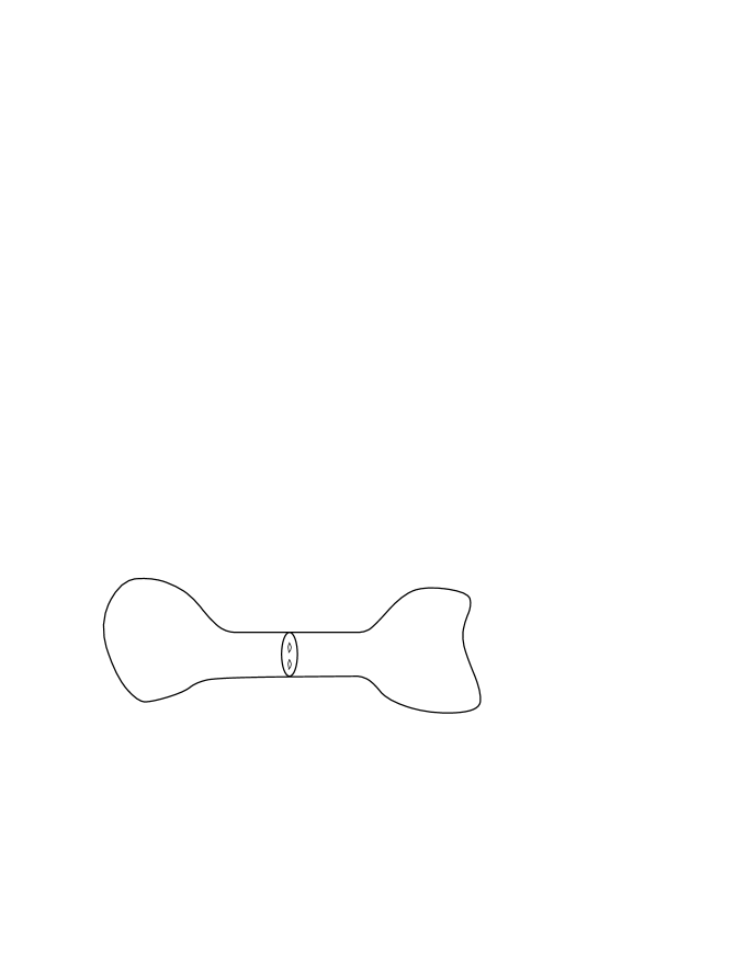
$Y$                                            $Z$

$\Sigma$

Figure 1: The split 3–manifold $X$

To stretch the collar of $\Sigma$, we introduce the notation

$$Y^{R} = Y\cup([0,R]\times\Sigma)$$

$$Z^{R} = Z\cup([-R,0]\times\Sigma)$$

for all $R\geq 1$. We also define $Y$ and $Z$ with infinite collars attached:

$$Y^{\infty} = Y\cup([0,\infty)\times\Sigma)$$

$$Z^{\infty} = Z\cup((-\infty,0]\times\Sigma).$$

Notice that since $\Phi\circ D_{A}=J\circ(S_{a}+{\frac{\partial}{\partial u}})\circ\Phi$, the operator $D_{A}$ has natural extensions to $Y^{R}$, $Z^{R}$, $Y^{\infty}$, and $Z^{\infty}$.

2.3 The spaces P⁺ and P^-

In this section we identify certain subspaces of the $L^{2}$ forms on $\Sigma$ associated to the operators $S_{a}$ and $D_{A}$. We first consider $L^{2}$ solutions to $D_{A}(\sigma,\tau)=0$ on $Y^{\infty}$ and $Z^{\infty}$. Since $S_{a}$ is elliptic on the closed surface $\Sigma$, its spectrum is discrete and each eigenspace is a finite-dimensional space of smooth forms.

Suppose $(\sigma,\tau)\in\Omega^{0+1}_{Y^{\infty}}\otimes{\mathbb{C}}^{2}$ is a solution to $D_{A}(\sigma,\tau)=0$ on $Y^{\infty}$. Following [3], write $\Phi(\sigma,\tau)=\sum c_{\lambda}(u)\phi_{\lambda}$ along $[0,\infty)\times\Sigma,$ where $\phi_{\lambda}\in\Omega^{0+1+2}_{\Sigma}\otimes{\mathbb{C}}^{2}$ is an eigenvector of $S_{a}$ with eigenvalue $\lambda.$ Since $\Phi\circ D_{A}=J\circ(S_{a}+\tfrac{\partial}{\partial u})\circ\Phi$, it follows by hypothesis that

$$0 = (S_{a}+\tfrac{\partial}{\partial u})(\Phi(\sigma,\tau))$$ (2.2)

$$= \sum_{\lambda}(\lambda c_{\lambda}+\tfrac{\partial c_{\lambda}}{\partial u})\phi_{\lambda}$$

hence

$$c_{\lambda}(u)=e^{-\lambda u}b_{\lambda}$$

for some constants $b_{\lambda}$. Thus $(\sigma,\tau)\in L^{2}(\Omega^{0+1}_{Y^{\infty}}\otimes{\mathbb{C}}^{2})$ if and only if $c_{\lambda}(u)=0$ for all $\lambda\leq 0.$

This implies that there is a one-to-one correspondence, given by restricting from $Y^{\infty}$ to $Y$, between the $L^{2}$ solutions to $D_{A}(\sigma,\tau)=0$ on $Y^{\infty}$ and the solutions to $D_{A}(\sigma,\tau)=0$ on $Y$ whose restriction to the boundary $\Sigma$ lie in the positive eigenspace $P^{+}_{a}\subset L^{2}(\Omega^{0+1+2}_{\Sigma}\otimes{\mathbb{C}}^{2})$ of $S_{a}$, defined by

$$P^{+}_{a}=\operatorname{span}_{L^{2}}\{\phi_{\lambda}\mid\lambda>0\}.$$

Recalling that $\Sigma=\partial Y=-\partial Z$, we obtain a similar one-to-one correspondence between the space of $L^{2}$ solutions to $D_{A}(\sigma,\tau)=0$ on $Z^{\infty}$ and the space of solutions to $D_{A}(\sigma,\tau)$ on $Z$ whose restriction to the boundary $\Sigma$ lie in the negative eigenspace $P^{-}_{a}\subset L^{2}(\Omega^{0+1+2}_{\Sigma}\otimes{\mathbb{C}}^{2})$ of $S_{a}$, defined by

$$P^{-}_{a}=\operatorname{span}_{L^{2}}\{\phi_{\lambda}\mid\lambda<0\}.$$

The spectrum of $S_{a}$ is symmetric and $J$ preserves the kernel of $S_{a}$ since $S_{a}J=-JS_{a}$. In fact, $J$ restricts to an isometry $J\co P^{+}_{a}\longrightarrow P^{-}_{a}$. The eigenspace decomposition of $S_{a}$ determines the orthogonal decomposition into closed subspaces

$$L^{2}(\Omega^{0+1+2}_{\Sigma}\otimes{\mathbb{C}}^{2})=P^{+}_{a}\oplus\ker S_{a}\oplus P^{-}_{a}.$$ (2.3)

The spaces $P^{\pm}_{a}$ are isotropic subspaces and are Lagrangian if and only if $\ker S_{a}=0$. Since $\Sigma$ bounds the 3–manifold $Y$ and the operator $D_{A}$ is defined on $Y$, it is not hard to see that the signature of the restriction of $iJ$ to $\ker S_{a}$ is zero. Hence $\ker S_{a}$ is a finite-dimensional sub-symplectic space of $L^{2}(\Omega^{0+1+2}_{\Sigma}\otimes{\mathbb{C}}^{2})$. The restrictions of the complex structure $J$ and the inner product to $\ker S_{a}$ depend on the Riemannian metric, whereas the symplectic structure $\omega(x,y)=\langle x,Jy\rangle$ depends on the orientation but not on the metric.

An important observation is that if $L\subset\ker S_{a}$ is any Lagrangian subspace, then $P^{+}_{a}\oplus L$ and $P^{-}_{a}\oplus L$ are infinite-dimensional Lagrangian subspaces of $L^{2}(\Omega^{0+1+2}_{\Sigma}\otimes{\mathbb{C}}^{2})$.

If $a\in\Omega^{1}_{\Sigma}\otimes su(2)$ is a flat connection, that is, if the curvature 2–form $F_{a}=da+a\wedge a$ is everywhere zero, then the kernel of $S_{a}$ consists of harmonic forms, ie, $S_{a}(\alpha,\beta,\gamma)=0$ if and only if $d_{a}\alpha=d_{a}\beta=d_{a}^{*}\beta=d_{a}^{*}\gamma=0$. The Hodge and de Rham theorems identify $\ker S_{a}$ with the cohomology group $H^{0+1+2}(\Sigma;{\mathbb{C}}^{2}_{a})$, where ${\mathbb{C}}^{2}_{a}$ denotes the local coefficient system determined by the holonomy representation of the flat connection $a$. Under this identification, the induced symplectic structure on $H^{0+1+2}(\Sigma;{\mathbb{C}}^{2}_{a})$ agrees with the direct sum of the symplectic structures on $H^{0+2}(\Sigma;{\mathbb{C}}^{2}_{a})$ and $H^{1}(\Sigma,{\mathbb{C}}^{2}_{a})$ given by the negative of the cup product. This is because the wedge products of differential forms induces the cup product on de Rham cohomology, and because of the formula

$$\omega(x,y)=\langle x,Jy\rangle=-\int_{\Sigma}x\wedge y=-(x\cup y)[\Sigma],$$

where the forms $x$ and $y$ are either both are 1–forms or 0– and 2–forms, respectively. In this formula, we have suppressed the notation for the complex inner product on ${\mathbb{C}}^{2}$ for the forms as well as in the cup product. Notice that $H^{0}(\Sigma;{\mathbb{C}}^{2}_{a})$ and $H^{2}(\Sigma;{\mathbb{C}}^{2}_{a})$ are Lagrangian subspaces of $H^{0+2}(\Sigma;{\mathbb{C}}^{2}_{a})$.

2.4 Limiting values of extended L² solutions and Cauchy data spaces

Our next task is to identify the Lagrangian of limiting values of extended $L^{2}$ solutions, and its infinite-dimensional generalization, the Cauchy data spaces, in the case when $A$ is a flat connection in cylindrical form on a 3–manifold $Y$ with boundary $\Sigma$.

Atiyah, Patodi and Singer define the space of limiting values of extended $L^{2}$ solutions to $D_{A}\phi=0$ to be a certain finite-dimensional Lagrangian subspace

$$L_{Y,A}\subset\ker S_{a},$$

where $a$ denotes the restriction of $A$ to the boundary. We give a brief description of this subspace and refer to [3, 20] for further details.

First we define the Cauchy data spaces; these will be crucial in our later analysis. We follow [29] closely; our terminology is derived from that article. In [6] it is shown that there is a well-defined, injective restriction map

$$r\co\ker\left(D_{A}\co L^{2}_{\frac{1}{2}}(\Omega^{0+1}_{Y}\otimes{\mathbb{C}}^{2})\to L^{2}_{-{\frac{1}{2}}}(\Omega^{0+1}_{Y}\otimes{\mathbb{C}}^{2})\right)\longrightarrow L^{2}(\Omega^{0+1+2}_{\Sigma}\otimes{\mathbb{C}}^{2}).$$ (2.4)

Unique continuation for the operator $D_{A}$ (which holds for any generalized Dirac operator) implies that $r$ is injective.

Definition 2.5.

The image of $r$ is a closed, infinite-dimensional Lagrangian subspace of $L^{2}(\Omega^{0+1+2}_{\Sigma}\otimes{\mathbb{C}}^{2})$. It is called the Cauchy data space of the operator $D_{A}$ on $Y$ and is denoted

$$\Lambda_{Y,A}.$$

Thus the Cauchy data space is the space of restrictions to the boundary of solutions to $D_{A}(\sigma,\tau)=0$. It is shown in [29] that $\Lambda_{Y,A}$ varies continuously with the connection $A$.

Definition 2.6.

The limiting values of extended $L^{2}$ solutions is defined as the symplectic reduction of $\Lambda_{Y,A}$ with respect to the isotropic subspace $P^{+}_{a}$, the positive eigenspace of $S_{a}$. Precisely,

$$L_{Y,A}=\operatorname{proj}_{\ker S_{a}}\left(\Lambda_{Y,A}\cap(P^{+}_{a}\oplus\ker S_{a})\right)=\frac{\Lambda_{Y,A}\cap(P^{+}_{a}\oplus\ker S_{a})}{\Lambda_{Y,A}\cap P^{+}_{a}}\subset\ker S_{a}.$$

This terminology comes from [3], where the restriction $r$ is used to identify the space of $L^{2}$ solutions of $D_{A}(\sigma,\tau)=0$ on $Y^{\infty}$ with the subspace $\Lambda_{Y,A}\cap P^{+}_{a}$, and the space of extended $L^{2}$ solutions with $\Lambda_{Y,A}\cap(P^{+}_{a}\oplus\ker S_{a})$. Thus $L_{Y,A}$ is the symplectic reduction of the extended $L^{2}$ solutions:

$$L_{Y,A}=\frac{\Lambda_{Y,A}\cap(P^{+}_{a}\oplus\ker S_{a})}{\Lambda_{Y,A}\cap P^{+}_{a}}\cong{\frac{\hbox{Extended }\ L^{2}\ \hbox{solutions}}{L^{2}\ \hbox{solutions}}}$$ (2.5)

We now recall a result of Nicolaescu on the “adiabatic limit” of the Cauchy data spaces [29]. To avoid some technical issues, we make the assumption $\Lambda_{Y,A}\cap P^{+}=0$; in the terminology of [29], this means that 0 is a non-resonance level for $D_{A}$ acting on $Y$. This assumption does not hold in general, but it does hold in all the cases considered in this article.

To set this up, replace $Y$ by $Y^{R}$ and extend $D_{A}$ to $Y^{R}$. This determines a continuous family $\Lambda^{R}_{Y,A}=\Lambda_{Y^{R},A}$ of Lagrangian subspaces of $L^{2}(\Omega^{0+1+2}_{\Sigma}\otimes{\mathbb{C}}^{2})$ by Lemma 3.2 of [14]. The corresponding subspace $L_{Y,A}^{R}$ of limiting values of extended $L^{2}$ solutions is independent of $R$.

Nicolaescu’s theorem asserts that as $R\to\infty$, $\Lambda^{R}_{Y,A}$ limits to a certain Lagrangian. Our assumption that 0 is a non-resonance level ensures that its limit is $L_{Y,A}\oplus P^{-}_{a}$. Recall from Equation (2.3) that $L^{2}(\Omega^{0+1+2}_{\Sigma}\otimes{\mathbb{C}}^{2})$ is decomposed into the orthogonal sum of $P^{+}_{a}$, $P^{-}_{a}$, and $\ker S_{a}$. Notice also that the definition of $L_{Y,A}$ in Equation (2.5) shows that it is independent of the collar length, ie, that

$$\hbox{proj}_{\ker S_{a}}\left(\Lambda^{R}_{Y,A}\cap(P^{+}_{a}\oplus\ker S_{a})\right)$$

is independent of $R$. This follows easily from the eigenspace decomposition of $S_{a}$ in Equation (2.2).

We now state Nicolaescu’s adiabatic limit theorem [29], as sharpened in [14].

Theorem 2.7 (Nicolaescu).

Assume that $\Lambda_{Y,A}\cap P^{+}_{a}=0$ (equivalently assume that there are no $L^{2}$ solutions to $D_{A}(\sigma,\tau)=0$ on $Y^{\infty}$). Let $L_{Y,A}\subset\ker S_{a}$ denote the limiting values of extended $L^{2}$ solutions. Then

$$\lim_{R\to\infty}\Lambda^{R}_{Y,A}=L_{Y,A}\oplus P^{-}_{a},$$

with convergence in the gap topology on closed subspaces, and moreover the path of Lagrangians

$$t\mapsto\begin{cases}\Lambda^{1/(1-t)}_{Y,A}&t<1\\ L_{Y,A}\oplus P^{-}_{a}&t=1\end{cases}$$

is continuous for $t\in[0,1]$ in the gap topology on closed subspaces.

Next we introduce some notation for the extended $L^{2}$ solutions. Although we use the terminology of extended $L^{2}$ solutions and limiting values from [3], it is more convenient for us to use the characterization of these solutions in terms of forms on $Y$ with $P^{+}_{a}\oplus\ker S_{a}$ boundary conditions.

Definition 2.8.

Let $\widetilde{V}_{A}$ be the space of extended $L^{2}$ solutions to $D_{A}(\sigma,\tau)=0$. This is defined by setting

$$\widetilde{V}_{A}=\{(\sigma,\tau)\in\Omega_{Y}^{0+1}\otimes{\mathbb{C}}^{2}\mid D_{A}(\sigma,\tau)=0\hbox{ and }r(\sigma,\tau)\in P^{+}_{a}\oplus\ker S_{a}\}.$$

Define also the limiting value map $p\co\widetilde{V}_{A}\longrightarrow\ker S_{a}$ by setting $p(\sigma,\tau)=\hbox{proj}_{\ker S_{a}}(r(\sigma,\tau))$ for $(\sigma,\tau)\in\widetilde{V}_{A}$, where $r$ is the restriction map of Equation (2.4). Notice that $p(\widetilde{V}_{A})=L_{Y,A}$. The choice of terminology is explained by Equation (2.5).

Let $\Theta$ denote the trivial connection on $Y$ and $\theta$ the trivial connection on $\Sigma=\partial Y.$ Let $\Lambda_{Y}=\Lambda_{Y,\Theta}$ and $L_{Y}=L_{Y,\Theta}$. The following theorem identifies $L_{Y},$ the limiting values of extended $L^{2}$ solutions to $D_{\Theta}(\sigma,\tau)=0$ on $Y$. Since $\theta$ is the trivial connection on $\Sigma$, $\ker S_{\theta}$ can be identified with the (untwisted) cohomology $H^{0+1+2}(\Sigma;{\mathbb{C}}^{2})$.

Theorem 2.9.

Suppose $Y$ is a compact, oriented, connected 3–manifold with connected boundary $\Sigma$. Let $\Theta$ be the trivial connection on $Y$ and $\theta$ the trivial connection on $\Sigma$. Identify $\ker S_{\theta}$ with $H^{0+1+2}(\Sigma;{\mathbb{C}}^{2})$ using the Hodge theorem. Then the space of the limiting values of extended $L^{2}$ solutions decomposes as

$$L_{Y}=H^{0}(\Sigma;{\mathbb{C}}^{2})\oplus\operatorname{Im}\left(H^{1}(Y;{\mathbb{C}}^{2})\to H^{1}(\Sigma;{\mathbb{C}}^{2})\right).$$

ProofProposition 4.2 of [20] says that if $D_{\Theta}(\sigma,\tau)=0$ and $(\sigma,\tau)$ has boundary conditions in $P^{+}_{\theta}\oplus\ker S_{\theta}$ (ie, if $(\sigma,\tau)\in\widetilde{V}$), then $d_{\Theta}\sigma=0$, $d_{\Theta}\tau=0$ and $d^{*}_{\Theta}\tau=0$. Regularity of solutions to this elliptic boundary problem ensures that $\sigma$ and $\tau$ are smooth forms.

If $r(\sigma,\tau)=(\alpha,\beta,\gamma)$, then $\alpha\in\Omega^{0}_{\Sigma}\otimes{\mathbb{C}}^{2}$ is a closed form whose cohomology class equals the restriction of the cohomology class on $Y$ represented by $\sigma$. Similarly $\beta\in\Omega^{1}_{\Sigma}\otimes{\mathbb{C}}^{2}$ represents the restriction of the cohomology class of $\tau$ to $\Sigma$. Since the projection to harmonic forms does not change the cohomology class of a closed form,

$$p(\tilde{V}) \subset \operatorname{Im}(H^{0+1}(Y;{\mathbb{C}}^{2})\to H^{0+1}(\Sigma;{\mathbb{C}}^{2}))\oplus H^{2}(\Sigma,{\mathbb{C}}^{2})$$

$$= H^{0}(\Sigma;{\mathbb{C}}^{2})\oplus\operatorname{Im}(H^{1}(Y;{\mathbb{C}}^{2})\to H^{1}(\Sigma;{\mathbb{C}}^{2}))\oplus H^{2}(\Sigma;{\mathbb{C}}^{2}).$$

All of $H^{0}(\Sigma;{\mathbb{C}}^{2})$ is contained in $p(\tilde{V})$, since constant 0–forms on $\Sigma$ extend over $Y$, and if $\sigma$ is a constant $0$ form on $Y$ then $(\sigma,0)\in\tilde{V}$ because its restriction to the boundary lies in $\ker S_{\theta}$. This implies that

$$p(\tilde{V})\subset H^{0}(\Sigma;{\mathbb{C}}^{2})\oplus\operatorname{Im}(H^{1}(Y;{\mathbb{C}}^{2})\to H^{1}(\Sigma;{\mathbb{C}}^{2})).$$

Since $p(\tilde{V})$ is Lagrangian, it is a half dimensional subspace of $H^{0+1+2}(\Sigma,{\mathbb{C}}^{2})$. Poincaré duality and the long exact sequence of the pair $(Y,\Sigma)$ show that $H^{0}(\Sigma;{\mathbb{C}}^{2})\oplus\operatorname{Im}(H^{1}(Y;{\mathbb{C}}^{2})\to H^{1}(\Sigma;{\mathbb{C}}^{2}))$ has the same dimension, so they are equal.

Suppose $A$ is a flat connection on $Y$ with restriction $a=A|_{\Sigma}.$ Denote the kernel of the limiting value map by $K_{A}=\ker(p\co\widetilde{V}_{A}\longrightarrow\ker S_{a})$. By definition, $K_{A}$ is the kernel of $D_{A}$ on $Y$ with $P^{+}$ boundary conditions, but it can be characterized in several other useful ways. The eigenvalue expansion of Equation (2.2) implies that every form in $K_{A}$ extends to an exponentially decaying $L^{2}$ solution to $D_{A}(\sigma,\tau)=0$ on $Y^{\infty}$. Moreover, the restriction map $r$ of Equation (2.4) sends $K_{A}$ injectively to $P^{+}_{a}$ by unique continuation, and $r(K_{A})=\Lambda_{Y,A}\cap P^{+}_{a}$. For more details, see the fundamental articles of Atiyah, Patodi, and Singer [3] and the book [6].

Suppose that $(\sigma,\tau)\in K_{A}$. Then Proposition 4.2 of [20] implies that $d_{A}\sigma=0$, $d_{A}\tau=0$ and $d_{A}^{*}\tau=0$. Since $A$ is an $SU(2)$ connection, we have that

$$d\langle\sigma,\sigma\rangle=\langle d_{A}\sigma,\sigma\rangle+\langle\sigma,d_{A}\sigma\rangle=0$$

pointwise. Thus the pointwise norm of $\sigma$ is constant. Since $\sigma$ extends to an $L^{2}$ form on $Y^{\infty}$, $\sigma=0$. Also $\tau$ is an $L^{2}$ harmonic 1–form on $Y^{\infty}$. In [3] it is shown that if $A$ is a flat connection then the space of $L^{2}$ harmonic 1–forms on $Y^{\infty}$ is isomorphic to

$$\operatorname{Im}\left(H^{1}(Y,\Sigma;{\mathbb{C}}^{2}_{A})\to H^{1}(Y;{\mathbb{C}}^{2}_{A})\right),$$

the image of the relative cohomology in the absolute. Hence there is a short exact sequence

$$0\to\operatorname{Im}\left(H^{1}(Y,\Sigma;{\mathbb{C}}^{2}_{A})\to H^{1}(Y;{\mathbb{C}}^{2}_{A})\right)\longrightarrow\widetilde{V}_{A}\longrightarrow L_{Y,A}\to 0.$$

More generally, for any subspace $Q\subset\ker S_{a}$, restricting $p$ to $\widetilde{V}_{A}\cap(P^{+}_{a}\oplus Q)$, one obtains the following very useful proposition.

Proposition 2.10.

Suppose that $A$ is a flat connection on a 3–manifold $Y$ with boundary $\Sigma$. Let $a$ be the restriction of $A$ to $\Sigma$. If $Q\subset\ker S_{a}$ is any subspace (not necessarily Lagrangian), then there is a short exact sequence

$$0\to\operatorname{Im}\left(H^{1}(Y,\Sigma;{\mathbb{C}}^{2}_{A})\to H^{1}(Y;{\mathbb{C}}^{2}_{A})\right)\longrightarrow\ker D_{A}(P^{+}_{a}\oplus Q)\smash{\mathop{\longrightarrow}\limits^{p}}L_{Y,A}\cap Q\to 0,$$

where $\ker D_{A}(P^{+}_{a}\oplus Q)$ consists of solutions to $D_{A}(\sigma,\tau)=0$ whose restrictions to the boundary lie in $P^{+}_{a}\oplus Q$.

If $Q=0$, then this gives the isomorphisms

$$\Lambda_{Y,A}\cap P^{+}_{a}\cong K_{A}\cong\operatorname{Im}\left(H^{1}(Y,\Sigma;{\mathbb{C}}^{2}_{A})\to H^{1}(Y;{\mathbb{C}}^{2}_{A})\right).$$

2.5 Spectral flow and Maslov index conventions

If $D_{t},\ t\in[0,1]$ is a 1–parameter family of self-adjoint operators with compact resolvents and with $D_{0}$ and $D_{1}$ invertible, the spectral flow $SF(D_{t})$ is the algebraic number of eigenvalues crossing from negative to positive along the path. For precise definitions, see [3] and [10]. In case $D_{0}$ or $D_{1}$ is not invertible, we adopt the $(-\varepsilon,-\varepsilon)$ convention to handle zero eigenvalues at the endpoints.

Definition 2.11.

Given a continuous 1–parameter family of self-adjoint operators with compact resolvents $D_{t},\ t\in[0,1]$, choose $\varepsilon>0$ smaller than the modulus of the largest negative eigenvalue of $D_{0}$ and $D_{1}$. Then the spectral flow $SF(D_{t})$ is defined to be the algebraic intersection number in $[0,1]\times{\mathbb{R}}$ of the track of the spectrum

$$\{(t,\lambda)\mid\ t\in[0,1],\ \lambda\in\hbox{Spec}(D_{t})\}$$

and the line segment from $(0,-\varepsilon)$ to $(1,-\varepsilon)$. The orientations are chosen so that if $D_{t}$ has spectrum $\{n+t\mid n\in{{\mathbb{Z}}}\}$ then $SF(D_{t})=1$.

The proof of the following proposition is clear.

Proposition 2.12.

With the convention set above, the spectral flow is additive with respect to composition of paths of operators. It is an invariant of homotopy rel endpoints of paths of self-adjoint operators. If $\dim\ker D_{t}$ is constant, then $SF(D_{t})=0.$

We will apply this definition to families of odd signature operators obtained from paths $A_{t}$ of $SU(2)$ connections. Suppose $A_{t}$ is a path of $SU(2)$ connections on the closed 3–manifold $X$ for $0\leq t\leq 1$. We denote by $SF(A_{t};X)$ the spectral flow of the family of odd signature operators $D_{A_{t}}$ on $\Omega^{0+1}_{X}\otimes{\mathbb{C}}^{2}.$ Since the space of all connections is contractible, the spectral flow $SF(A_{t};X)$ depends only on the endpoints $A_{0}$ and $A_{1}$ and we shall occasionally adopt the notation $SF(A_{0},A_{1};X)$ to emphasize this point.

We next introduce a compatible convention for the Maslov index [12]. A good reference for these ideas is Nicolaescu’s article [29]. Let $H$ be a symplectic Hilbert space with compatible almost complex structure $J$. A pair of Lagrangians $(L,M)$ in $H$ is called Fredholm if $L+M$ is closed and both $\dim(L\cap M)$ and $\operatorname{codim}(L+M)$ are finite. We will say that two Lagrangians are transverse if they intersect trivially.

Consider a continuous path $(L_{t},M_{t})$ of Fredholm pairs of Lagrangians in $H$. Here, continuity is measured in the gap topology on closed subspaces. If $L_{i}$ is transverse to $M_{i}$ for $i=0,1$, then the Maslov index $\operatorname{Mas}(L_{t},M_{t})$ is the number of times the two Lagrangians intersect, counted with sign and multiplicity. We choose the sign so that if $(L,M)$ is a fixed Fredholm pair of Lagrangians such that $e^{sJ}L$ and $M$ are transverse for all $0\neq s\in[-\varepsilon,\varepsilon]$, then $\operatorname{Mas}(e^{\varepsilon(2t-1)J}L,M)=\dim(L\cap M)$. A precise definition is given in [29] and more general properties of the Maslov index are detailed in [9, 25].

Extending the Maslov index to paths where the pairs at the endpoints are not transverse requires more care. We use $e^{sJ}$, the 1–parameter group of symplectic transformations associated to $J$, to make them transverse. If $L$ and $M$ are any two Lagrangians, then $e^{sJ}L$ and $M$ are transverse for all small nonzero $s$. By [18], the set of Fredholm pairs is open in the space of all pairs of Lagrangians. Hence, if $(L,M)$ is a Fredholm pair, then so is $(e^{sJ}L,M)$ for all $s$ small.

Definition 2.13.

Given a continuous 1–parameter family of Fredholm pairs of Lagrangians $(L_{t},M_{t}),\ t\in[0,1],$ choose $\varepsilon>0$ small enough that

1. $e^{sJ}L_{i}$ is transverse to $M_{i}$ for $i=0,1$ and $0<s\leq\varepsilon$, and

2. $(e^{sJ}L_{t},M_{t})$ is a Fredholm pair for all $t\in[0,1]$ and all $0\leq s\leq\varepsilon$.

Then define the Maslov index of the pair $(L_{t},M_{t})$ to be the Maslov index of $(e^{\varepsilon J}L_{t},M_{t})$.

The proof of the following proposition is easy.

Proposition 2.14.

With the conventions set above, the Maslov index is additive with respect to composition of paths. It is an invariant of homotopy rel endpoints of paths of Fredholm pairs of Lagrangians. Moreover, if $\dim(L_{t}\cap M_{t})$ is constant, then $\operatorname{Mas}(L_{t},M_{t})=0$.

For 1–parameter families of Lagrangians $(L_{t},M_{t})$ which are transverse except at one of the endpoints, the Maslov index $\operatorname{Mas}(L_{t},M_{t})$ is often easy to compute.

Proposition 2.15.

Let $(L_{t},M_{t}),\ t\in[0,1],$ be a continuous 1–parameter family of Fredholm pairs of Lagrangians which are transverse for $t\neq 0.$ Suppose $s\co{\mathbb{R}}\to{\mathbb{R}}$ is a smooth function with $s(0)=0$ and $s^{\prime}(0)\neq 0.$ Choose $\delta>0$ so that $s(t)$ is strictly monotone on $[0,\delta]$ and $\varepsilon>0$ with $\varepsilon<|s(\delta)|$ and $\varepsilon<|s(-\delta)|.$ Suppose further that, for all $-\varepsilon\leq r\leq\varepsilon$ and all $0\leq t\leq\delta,$ the pair $(e^{rJ}L_{t},M_{t})$ satisfies

$$\dim(e^{rJ}L_{t}\cap M_{t})=\begin{cases}\dim(L_{0}\cap M_{0})&\text{if }r=s(t)\\ 0&\text{otherwise.}\end{cases}$$

Then

$$\operatorname{Mas}(L_{t},M_{t})=\begin{cases}-\dim(L_{0}\cap M_{0})&\text{if }s^{\prime}(0)>0\\ 0&\text{if }s^{\prime}(0)<0.\end{cases}$$

ProofWrite

$$\operatorname{Mas}(L_{t},M_{t})=\operatorname{Mas}(L_{t},M_{t};\ 0\leq t\leq\delta)+\operatorname{Mas}(L_{t},M_{t};\ \delta\leq t\leq 1).$$

Since $L_{t}$ and $M_{t}$ are transverse for $t\in[\delta,1]$, it follows that

$$\operatorname{Mas}(L_{t},M_{t};\ \delta\leq t\leq 1)=0.$$

The convention for dealing with non-transverse endpoints now applies to show that

$$\operatorname{Mas}(L_{t},M_{t})=\operatorname{Mas}(L_{t},M_{t};\ 0\leq t\leq\delta)=\operatorname{Mas}(e^{\varepsilon J}L_{t},M_{t};\ 0\leq t\leq\delta).$$

If $s^{\prime}(0)<0,$ then $s(t)$ is monotone decreasing on $[0,\delta]$ and the hypotheses imply that $e^{\varepsilon J}L_{t}$ and $M_{t}$ are transverse for $t\in[0,\delta]$. Hence $\operatorname{Mas}(L_{t},M_{t})=0$ as claimed.

On the other hand, if $s^{\prime}(0)>0,$ then we write

$$\operatorname{Mas}(e^{\varepsilon J}L_{t},M_{t};\ 0\leq t\leq\delta) = \operatorname{Mas}(e^{\varepsilon(1-2t)J}L_{0},M_{0};\ 0\leq t\leq 1)$$

$$+\operatorname{Mas}(e^{-\varepsilon J}L_{t},M_{t};\ 0\leq t\leq\delta)$$

$$+\operatorname{Mas}(e^{\varepsilon(2t-1)J}L_{\delta},M_{\delta};\ 0\leq t\leq 1).$$

Since $s(t)$ is now monotone increasing on $[0,\delta]$, the hypotheses imply that $e^{-\varepsilon J}L_{t}$ and $M_{t}$ are transverse for $t\in[0,\delta]$. Furthermore, by choosing $\varepsilon$ smaller, if necessary, we can assume that $e^{\varepsilon(2t-1)J}L_{\delta}$ and $M_{\delta}$ are transverse for all $t\in[0,1]$. Hence

$$\operatorname{Mas}(L_{t},M_{t}) = \operatorname{Mas}(e^{\varepsilon(1-2t)J}L_{0},M_{0})$$

$$= -\operatorname{Mas}(e^{\varepsilon(2t-1)J}L_{0},M_{0})=-\dim(L_{0},M_{0})$$

by our sign convention. RemarkThere is a similar result for pairs $(L_{t},M_{t})$ which are transverse for $t\neq 1$. If $s(t)$ is a smooth function satisfying the analogous conditions, namely that $s(1)=0,\ s^{\prime}(1)\neq 0$ and

$$\dim(e^{rJ}L_{t}\cap M_{t})=\begin{cases}\dim(L_{1}\cap M_{1})&\text{if }r=s(t)\\ 0&\text{otherwise,}\end{cases}$$

then

$$\operatorname{Mas}(L_{t},M_{t})=\begin{cases}\dim(L_{1}\cap M_{1})&\text{if }s^{\prime}(1)<0\\ 0&\text{if }s^{\prime}(1)>0.\end{cases}$$

The details of the proof are left to the reader.

2.6 Nicolaescu’s decomposition theorem for spectral flow

The spectral flow and Maslov index are related by the following result of Nicolaescu, which holds in the more general context of neck compatible generalized Dirac operators. The following is the main theorem of [29], as extended in [12], stated in the context of the odd signature operator $D_{A}$ on a 3–manifold.

Theorem 2.16.

Suppose $X$ is a 3–manifold decomposed along a surface $\Sigma$ into two pieces $Y$ and $Z$, with $\Sigma$ oriented so that $\Sigma=\partial Y=-\partial Z$. Suppose $A_{t}$ is a continuous path of $SU(2)$ connections on $X$ in cylindrical form in a collar of $\Sigma$. Let $\Lambda_{Y}(t)=\Lambda_{Y,A_{t}}$ and $\Lambda_{Z}(t)=\Lambda_{Z,A_{t}}$ be the Cauchy data spaces associated to the restrictions of $D_{A_{t}}$ to $Y$ and $Z.$ Then $(\Lambda_{Y}(t),\Lambda_{Z}(t))$ is a Fredholm pair of Lagrangians and

$$SF(A_{t};X)=\operatorname{Mas}(\Lambda_{Y}(t),\Lambda_{Z}(t)).$$

There is also a theorem for manifolds with boundary, see [30, 13]. This requires the introduction of boundary conditions. The following is not the most general notion, but suffices for our exposition. See [6, 25] for a more detailed analysis of elliptic boundary conditions.

Definition 2.17.

Let $D_{A}$ be the odd signature operator twisted by a connection $A$ on a 3–manifold $Y$ with non-empty boundary $\Sigma$. A subspace $\widetilde{P}\subset L^{2}(\Omega^{0+1+2}_{\Sigma}\otimes{\mathbb{C}}^{2})$ is called a self-adjoint Atiyah–Patodi–Singer (APS) boundary condition for $D_{A}$ if $\widetilde{P}$ is a Lagrangian subspace and if, in addition, $\widetilde{P}$ contains all the eigenvectors of the tangential operator $S_{a}$ which have sufficiently large positive eigenvalue as a finite codimensional subspace. In other words, there exists a positive number $q$ so that

$$\{\phi_{\lambda}\mid S_{a}(\phi_{\lambda})=\lambda\phi_{\lambda}\hbox{ and }\lambda>q\}\subset\widetilde{P}$$

with finite codimension.

Lemma 2.18.

Suppose that $X=Y\cup_{\Sigma}Z$ and $A_{0}$, $A_{1}$ are $SU(2)$ connections in cylindrical form on the collar of $\Sigma$ as above. Let $\widetilde{P}_{0}$ (resp. $\widetilde{P}_{1}$) be a self-adjoint APS boundary condition for $D_{A_{0}}$ (resp. $D_{A_{1}}$) restricted to $Y$.

Then

$$(\Lambda_{Y,A_{0}},\Lambda_{Z,A_{1}}),\ (\Lambda_{Y,A_{0}},\widetilde{P}_{1}),\ (J\widetilde{P}_{0},\Lambda_{Z,A_{1}}),\ \text{ and }(J\widetilde{P}_{0},\widetilde{P}_{1})$$

are Fredholm pairs.

ProofLet $S_{a_{0}}$ and $S_{a_{1}}$ denote the tangential operators of $D_{A_{0}}$ and $D_{A_{1}}$. It is proved in [6] that

1. The $L^{2}$–orthogonal projections to $\Lambda_{Y,A_{0}}$ and $\Lambda_{Y,A_{1}}$ are zeroth–order pseudo-differential operators whose principal symbols are just the projections onto the positive eigenspace of the principal symbols of $S_{a_{0}}$ and $S_{a_{1}}$, respectively.

2. If $Q_{0}$ and $Q_{1}$ denote the $L^{2}$–orthogonal projections to the positive eigenspans of $S_{a_{0}}$ and $S_{a_{1}}$, respectively, then $Q_{0}$ and $Q_{1}$ are zeroth–order pseudo-differential operators whose principal symbols are also the projections onto the positive eigenspaces of the principal symbols of $S_{a_{0}}$ and $S_{a_{1}}$.

From the definition one sees that the difference $S_{a_{0}}-S_{a_{1}}$ is a zeroth order differential operator, and in particular the principal symbols of $S_{a_{0}}$ and $S_{a_{1}}$ coincide. Hence

$$\sigma(Q_{0})=\sigma(Q_{1})=\sigma(\text{proj}_{\Lambda_{Y,A_{0}}})=\sigma(\text{proj}_{\Lambda_{Y,A_{1}}}),$$

where $\sigma$ denotes the principal symbol. Moreover, $Q_{i}$ and the projection to $\widetilde{P}_{i}$ differ by a finite-dimensional projection. This implies that the projections to $\Lambda_{Y,A_{0}}$, $\Lambda_{Y,A_{1}}$, $\widetilde{P}_{0}$, and $\widetilde{P}_{1}$ are compact perturbations of $Q_{0}$. The lemma follows from this and the fact that viewed from the “$Z$ side,” the roles of the positive and negative spectral projections are reversed.

It follows from the results of [3] (see also [6]) that restricting the domain of $D_{A}$ to $r^{-1}(\widetilde{P})\subset L^{2}_{1}(\Omega^{0+1}_{Y}\otimes{\mathbb{C}}^{2})$ yields a self-adjoint elliptic operator. Moreover, unique continuation for solutions to $D_{A}(\sigma,\tau)=0$ shows that the kernel of $D_{A}$ on $Y$ with APS boundary conditions $\widetilde{P}$ is mapped isomorphically by the restriction map $r$ to $\Lambda_{Y,A}\cap\widetilde{P}$.

A generalization of Theorem 2.16, which is also due to Nicolaescu (see [30] and [12]), states the following.

Theorem 2.19 (Nicolaescu).

Suppose $Y$ is a 3–manifold with boundary $\Sigma.$ If $A_{t}$ is a path of connections on $Y$ in cylindrical form near $\Sigma$ and $\widetilde{P}_{t}$ is a continuous family of self-adjoint APS boundary conditions, then the spectral flow $SF(A_{t};Y;\widetilde{P}_{t})$ is well defined and

$$SF(A_{t};Y;\widetilde{P}_{t})=\operatorname{Mas}(\Lambda_{Y}(t),\widetilde{P}_{t}).$$

3 Splitting the spectral flow for Dehn surgeries

In this paper, the spectral flow theorems described in the previous section will be applied to homology 3–spheres $X$ obtained by Dehn surgery on a knot, so $X$ is decomposed as $X=Y\cup_{\Sigma}Z$ where $Y=D^{2}\times S^{1}$ and $\Sigma=\partial Y$ is the 2–torus. In our examples, $Z$ will be the complement of a knot in $S^{3}$, but the methods work just as well for knot complements in other homology spheres.

This section is devoted to proving a splitting theorem for ${\mathbb{C}}^{2}$–spectral flow of the odd signature operator for paths of $SU(2)$ connections with certain properties. In the end, the splitting theorem expresses the spectral flow as a sum of two terms, one involving $Z$ and the other involving $Y$.

3.1 Decomposing X along a torus

We make the following assumptions, which will hold for the rest of this article.

1. The surface $\Sigma$ is the torus

   $$T=S^{1}\times S^{1}=\{(e^{ix},e^{iy})\},$$

   oriented so that the 1–forms $dx$ and $dy$ are ordered as $\{dx,dy\}$ and with the product metric, where the unit circle $S^{1}\subset{\mathbb{C}}$ is given the standard metric. The torus $T$ contains the two curves

   $$\mu=\{(e^{ix},1)\}\quad\text{and}\quad\lambda=\{(1,e^{iy})\},$$

   and $\pi_{1}(T)$ is the free abelian group generated by these two loops.

2. The 3–manifold $Y$ is the solid torus

   $$Y=D^{2}\times S^{1}=\{(re^{ix},e^{iy})\mid 0\leq r\leq 1\},$$

   oriented so that $drdxdy$ is a positive multiple of the volume form when $r>0$. The fundamental group $\pi_{1}(Y)$ is infinite cyclic generated by $\lambda$ and the curve $\mu$ is trivial in $\pi_{1}Y$ since it bounds the disc $D^{2}\times\{1\}$. There is a product metric on $Y$ such that a collar neighborhood of the boundary may be isometrically identified with $[-1,0]\times T$ and $\partial Y=\{0\}\times T$. The form $dy$ is a globally defined 1–form on $Y$, whereas the form $dx$ is well-defined off the core circle of $Y$ (ie, the set where $r=0$).

3. The 3–manifold $Z$ is the complement of an open tubular neighborhood of a knot in a homology sphere. Moreover, we assume that the identification of $T$ with $\partial Z$ takes the loop $\lambda$ to a null-homologous loop in $Z$.

   There is a metric on $Z$ such that a collar neighborhood of the boundary may be isometrically identified with $[0,1]\times T$. As oriented manifolds, $\partial Z=-\{0\}\times T$. The form $dx$ on $\partial Z$ extends to a closed 1–form on $Z$ generating the first cohomology $H^{1}(Z;{\mathbb{R}})$ which we continue to denote $dx$.

4. The closed 3–manifold $X=Y\cup_{T}Z$ is a homology sphere. The metric on $X$ is compatible with those on $Z$ and $Y$ and $T$ is identified with the set $\{0\}\times T$ in the neck.

3.2 Connections in normal form and the moduli space of T

Flat connections on the torus play a central role here, and in this subsection we describe a 2–parameter family of flat connections on the torus and discuss its relation to the flat moduli space.

For notational convenience, we identify elements of $SU(2)$ with unit quaternions via

$$\begin{pmatrix}\alpha&\beta\\ -\bar{\beta}&\bar{\alpha}\end{pmatrix}\leftrightarrow\alpha+\beta j$$

where $\alpha,\beta\in{\mathbb{C}}$ satisfy $|\alpha|^{2}+|\beta|^{2}=1$. The Lie algebra $su(2)$ is then identified with the purely imaginary quaternions

$$\begin{pmatrix}ix&y+iz\\ -y+iz&-ix\end{pmatrix}\leftrightarrow xi+yj+zk$$

for $x,y,z\in{\mathbb{R}}$.

With these notational conventions, the action of $su(2)$ on ${\mathbb{C}}^{2}$ can be written in the form

$$(ix+jy+kz)\cdot(v_{1}e_{1}+v_{2}e_{2})=(ixv_{1}+(y+iz)v_{2})e_{1}-((y-iz)v_{1}+ixv_{2})e_{2}.$$

In particular,

$$xi\cdot(v_{1}e_{1}+v_{2}e_{2})=ixv_{1}e_{1}-ixv_{2}e_{2}.$$ (3.1)

This corresponds to the standard inclusion $U(1)\subset SU(2)$ sending $\alpha\in U(1)$ to ${\rm diag}(\alpha,\alpha^{-1})\in SU(2)$. On the level of Lie algebras, this is the inclusion $u(1)\subset su(2)$ sending $ix$ to ${\rm diag}(ix,-ix)$.

Definition 3.1.

For $(m,n)\in{\mathbb{R}}^{2}$, let $a_{m,n}=-midx-nidy$ and define the connections in normal form on $T$ to be the set

$${\mathcal{A}}_{\rm nf}(T)=\{a_{m,n}\mid(m,n)\in{\mathbb{R}}^{2}\}.$$

An $SU(2)$ connection $A$ on $Z$ or $Y$ is said to be in normal form along the boundary if it is in cylindrical form on the collar neighborhood of $T$ and its restriction to the boundary is in normal form.

Notice that if $a=a_{m,n},$ then $\operatorname{hol}_{a}(\mu)=e^{2\pi im}$ and $\operatorname{hol}_{a}(\lambda)=e^{2\pi in}$. The relevance of connections in normal form is made clear by the following proposition, which follows from a standard gauge fixing argument. We will call a connection diagonal if its connection 1–form takes values in the diagonal Lie subalgebra $u(1)\subset su(2)$.

Proposition 3.2.

Any flat $SU(2)$ connection on $T$ is gauge equivalent to a diagonal connection. Moreover, any flat diagonal $SU(2)$ connection on $T$ is gauge equivalent via a gauge transformation $g\co T\to U(1)\subset SU(2)$ to a connection in normal form, and the normal form connection is unique if $g$ is required to be homotopic to the constant map $\operatorname{id}\co T\to\{\operatorname{id}\}\subset U(1)$.

We will introduce a special gauge group for the set of connections in normal form in Section 4.1, but for now note that any constant gauge transformation of the form $\cos(s)j+\sin(s)k$ acts on ${\mathcal{A}}_{\rm nf}(T)$ by sending $a_{m,n}$ to $a_{-m,-n}$. Alternatively, one can view this as interchanging the complex conjugate eigenvalues of the $SU(2)$ matrices in the holonomy representation.

For any manifold $X$ and compact Lie group $G$, denote by ${\mathfrak{R}}_{G}(X)$ the space of conjugacy classes of representations $\rho\co\pi_{1}X\to G,$ ie,

$${\mathfrak{R}}_{G}(X)=\mbox{Hom}(\pi_{1}X,G)/\mbox{conjugation},$$

and denote by ${\mathfrak{M}}_{G}(X)$ the space of flat connections on principal $G$–bundles over $X$ modulo gauge transformations of those bundles. In all cases considered here, $G=SU(n),\ n=2,3$ and $\dim X\leq 3$, so all $G$–bundles over $X$ are necessarily trivial. The association to each flat connection its holonomy representation provides a homeomorphism

$$\operatorname{hol}\co{\mathfrak{M}}_{G}(X)\stackrel{{\scriptstyle\cong}}{{\longrightarrow}}{\mathfrak{R}}_{G}(X),$$

so we will use whichever interpretation is convenient.

By identifying ${\mathcal{A}}_{\rm nf}(T)$ with ${\mathbb{R}}^{2}$, the moduli space ${\mathfrak{M}}_{SU(2)}(T)$ of flat connections (modulo the full gauge group) can be identified with the quotient of ${\mathbb{R}}^{2}$ by the semidirect product of ${\mathbb{Z}}/2$ with ${\mathbb{Z}}^{2}$, where ${\mathbb{Z}}/2$ acts by reflections through the origin and ${\mathbb{Z}}^{2}$ acts by translations. The quotient map is a branched covering. Indeed, setting $f(m,n)=[\operatorname{hol}_{a_{m,n}}\co\pi_{1}T\to SU(2)]$ for $(m,n)\in{\mathbb{R}}^{2}$ defines the branched covering map

$$f\co{\mathbb{R}}^{2}\to{\mathfrak{R}}_{SU(2)}(T).$$ (3.2)

Since the connection 1–form of any $a\in{\mathcal{A}}_{\rm nf}(T)$ takes values in $u(1)\subset su(2)$, the twisted cohomology splits

$$H^{0+1+2}(T;{\mathbb{C}}^{2}_{a})=H^{0+1+2}(T;{\mathbb{C}}_{\hat{a}})\oplus H^{0+1+2}(T;{\mathbb{C}}_{-\hat{a}}),$$

where $\pm\hat{a}$ are the $u(1)$ connections given by the reduction of the bundle. Similarly, the de Rham operator splits as

$$S_{a}=S_{\hat{a}}\oplus S_{-\hat{a}},$$ (3.3)

where $S_{\pm\hat{a}}\co\Omega^{0+1+2}_{T}\otimes{\mathbb{C}}\to\Omega^{0+1+2}_{T}\otimes{\mathbb{C}}$ are the de Rham operators associated to the $u(1)$ connections $\pm\hat{a}$.

We leave the following cohomology calculations to the reader. (See Equation (2.1) for the definition of $\operatorname{span}_{{\mathbb{C}}^{2}}$.)

1. The flat connection $a_{m,n}\in{\mathcal{A}}_{\rm nf}(T)$ is gauge equivalent to the trivial connection if and only if $(m,n)\in{\mathbb{Z}}^{2}$. Moreover,

   $$H^{0+1+2}(T;{\mathbb{C}}^{2}_{a})=\begin{cases}0&\text{if $(m,n)\not\in{\mathbb{Z}}^{2}$,}\\ \operatorname{span}_{{\mathbb{C}}^{2}}\{1,dx,dy,dxdy\}&\text{if $(m,n)=(0,0)$.}\end{cases}$$ (3.4)

2. If $A$ is a flat $SU(2)$ connection on $Y$ in normal form along the boundary (so $A|_{T}=a_{m,n}=-midx-nidy$ with $m\in{\mathbb{Z}}$), then $A$ is gauge equivalent to the trivial connection if and only if $n\in{\mathbb{Z}}$. Moreover,

   $$H^{0+1}(Y;{\mathbb{C}}^{2}_{A})=\begin{cases}0&\text{if $n\not\in{\mathbb{Z}}$,}\\ \operatorname{span}_{{\mathbb{C}}^{2}}\{1,dy\}&\text{if $n=0$}\end{cases}$$ (3.5)

3. For the trivial connection $\Theta$ on $Z$, the coefficients are untwisted and $H^{0+1}(Z;{\mathbb{C}}^{2})=\operatorname{span}_{{\mathbb{C}}^{2}}\{1,dx\}$.

In terms of the limiting values of extended $L^{2}$ solutions, these computations together with Theorem 2.9 give the following result.

Proposition 3.3.

The spaces of limiting values of extended $L^{2}$ solutions for the trivial connection on $Y$ and $Z$ are $L_{Y}=\operatorname{span}_{{\mathbb{C}}^{2}}\{1,\ dy\}$ and $L_{Z}=\operatorname{span}_{{\mathbb{C}}^{2}}\{1,dx\}$ respectively.

3.3 Extending connections in normal form on T over Y

The main technical difficulty in the present work has at its core the special nature of the trivial connection. We begin by specifying a 2–parameter family of connections on $Y$ near $\Theta$ which extend the connections on normal form on $T$. We will use these connections to build paths of connections on $X$ which start at the trivial connection and, at first, move away in a specified way that is independent of $Z$ and $Y$ except through the homological information in the identification of their boundaries (which determine our coordinates on $T$).

Choose once and for all a smooth non-decreasing cutoff function $q\co[0,1]\to[0,1]$ with $q(r)=0$ for $r$ near $0$ and $q(r)=1$ for $r$ near enough to $1$ that $(re^{ix},e^{iy})$ lies in the collar neighborhood of $T$.

For each point $(m,n)\in{\mathbb{R}}^{2}$, let $A_{m,n}$ be the connection in normal form on the solid torus $Y$ whose value at the point $(re^{ix},e^{iy})$ is

$$A_{m,n}(re^{ix},e^{iy})=-q(r)midx-nidy.$$ (3.6)

This can be thought of as a $U(1)$ connection, or as an $SU(2)$ connection using quaternionic notation. Notice that $A_{m,n}$ is flat if and only if $m=0$, and in general is flat away from an annular region in the interior of $Y$.

3.4 Paths of connections on X and adiabatic limits at ${\Theta}$

Suppose $X$ is a homology 3–sphere decomposed as $X=Y\cup_{T}Z.$ For the rest of this section, we will suppose that $A_{t},\ t\in[0,1]$ is a continuous path of $SU(2)$ connections on $X$ satisfying the following properties:

1. $A_{0}=\Theta$, the trivial connection on $X$, and $A_{1}$ is a flat connection on $X$.

2. The restriction of $A_{t}$ to the neck is a path of cylindrical normal form connections

   $$A_{t}|_{[-1,1]\times T}=a_{m_{t},n_{t}}$$

   for some piecewise smooth path $(m_{t},n_{t})$ in ${\mathbb{R}}^{2}$ with $(m_{t},n_{t})\not\in{\mathbb{Z}}^{2}$ for $0<t\leq 1$.

3. There exists a small number $\delta>0$ such that, for $0<t\leq\delta$,

   1. $(m_{t},n_{t})=(t,0)$,

   2. $A_{t}|_{Z}=-tidx$ and $A_{t}|_{Y}=-q(r)tidx$, and

   3. $\Delta_{Z}(e^{i2\pi t})\neq 0,$ where $\Delta_{Z}$ denotes the Alexander polynomial of $Z$.

Most of the time we will assume that the restriction of $A_{t}$ to $Z$ is flat for all $t$, but this is not a necessary hypothesis in Theorem 3.9. This extra bit of generality can be useful in contexts when the space ${\mathfrak{R}}_{SU(2)}(Z)$ is not connected.

The significance of the condition involving the Alexander polynomial is made clear by the following lemma and corollary.

Lemma 3.4.

If $A_{t}$ is a path of connections satisfying conditions 1–3 above and if $\delta>0$ is the constant in condition 3, then $H^{1}(Z,T;{\mathbb{C}}^{2}_{A_{t}})=0$ for $0\leq t\leq\delta$.

Sketch of ProofFor $A_{0}=\Theta,$ the trivial connection, this follows from the long exact sequence in cohomology of the pair $(Z,T)$ for $t=0$. Using the Fox calculus to identify the Alexander matrix with the differential on 1–cochains in the infinite cyclic cover of $Z$ proves the lemma for $0<t\leq\delta$. A very similar computation is carried out in [26].

Corollary 3.5.

With the same hypotheses as above, the $L^{2}$ kernel of $D_{A_{t}}$ on $Z^{\infty}$ is trivial for $0\leq t\leq\delta$. Equivalently, letting $\Lambda_{Z}(t)=\Lambda_{Z,A_{t}}$, then for $0\leq t\leq\delta$,

$$\Lambda_{Z}(t)\cap P^{-}_{a_{t}}=0.$$

Furthermore, letting $\Lambda^{R}_{Z}(t)=\Lambda_{Z^{R},A_{t}}$,

$$\lim_{R\to\infty}\Lambda^{R}_{Z}(t)=\begin{cases}L_{Z}\oplus P^{+}_{\theta}&\text{if $t=0$}\\ P^{+}_{a_{t}}&\text{if $0<t\leq\delta$.}\end{cases}$$

ProofThe first claim follows immediately from Proposition 2.10 applied to $Z$ with $K=0$. (The orientation conventions, as described in Section 2.3 explain why $P^{-}$ is used instead of $P^{+}$.) In the terminology of [29], this means that $0$ is a non-resonance level for $D_{A_{t}}$ for $0\leq t\leq\delta$. Applying Theorem 2.7, Theorem 2.9, and Equation (3.4) gives the second claim.

3.5 Harmonic limits of positive and negative eigenvectors

In this section, we investigate some limiting properties of the eigenvectors of $S_{a}$ where $a$ ranges over a neighborhood of the trivial connection $\theta$ in the space of connections in normal form on $T$.

Let $s\in{\mathbb{R}}$ be a fixed number. (Throughout this subsection, $s$ is a fixed angle. In Theorem 3.8, the value $s=0$ is used.) Consider the path of connections

$$a_{t}=-t\cos(s)idx-t\sin(s)idy$$

for $0\leq t\leq\delta$. Notice that $a_{t}$ is a path of connections in normal form approaching the trivial connection $\theta$ and the angle of approach is $s$.

The path of operators $S_{a_{t}}$ is an analytic (in $t$) path of elliptic self-adjoint operators. It follows from the results of analytic perturbation theory that $S_{a_{t}}$ has a spectral decomposition with analytically varying eigenvectors and eigenvalues (see [18, 23]). By Equation (3.4) we have

$$\dim(\ker S_{a_{t}})=\begin{cases}8&\text{if $t=0$}\\ 0&\text{if $0<t\leq\delta$}\end{cases}$$

and

$$\ker S_{\theta}=\operatorname{span}_{{\mathbb{C}}^{2}}\{1,\ dx,\ dy,\ dxdy\}.$$

Since the spectrum of $S_{a_{t}}$ is symmetric, it follows that for $t>0$ there are four linearly independent positive eigenvectors and four negative eigenvectors of $S_{a_{t}}$ whose eigenvalues limit to $0$ as $t\to 0^{+}$, ie, the eigenvectors limit to (untwisted) ${\mathbb{C}}^{2}$–valued harmonic forms. More precisely, there exist 4–dimensional subspaces $K^{+}_{s}$ and $K^{-}_{s}$ of $\ker S_{\theta}$ so that

$$\lim_{t\to 0^{+}}P^{+}_{a_{t}}=K^{+}_{s}\oplus P^{+}_{\theta}\quad\text{and}\quad\lim_{t\to 0^{+}}P^{-}_{a_{t}}=K^{-}_{s}\oplus P^{-}_{\theta}.$$

In particular, the paths of Lagrangians

$$t\mapsto\begin{cases}K^{+}_{s}\oplus P^{+}_{\theta}&\hbox{ if }t=0\\ P^{+}_{a_{t}}&\hbox{ if }0<t\leq 1\\ \end{cases}\quad\text{ and }\quad t\mapsto\begin{cases}K^{-}_{s}\oplus P^{-}_{\theta}&\hbox{ if }t=0\\ P^{-}_{a_{t}}&\hbox{ if }0<t\leq 1\\ \end{cases}$$

are continuous.

The finite-dimensional Lagrangian subspace $K^{+}_{s}$ will be used to extend the boundary conditions $P^{+}_{a}$ to a continuous family of boundary conditions up to $\theta$. Similarly, $K^{-}_{s}$ will be used to extend the boundary conditions $P^{-}_{a}$. The next proposition gives a useful description of these spaces.

Proposition 3.6.

Define the 1–form $\xi_{s}=-\cos(s)idx-\sin(s)idy.$ Consider the family of connections on $T$ given by $a_{t}=t\xi_{s}$ for $t\in[0,\delta]$. If $K^{+}_{s}$ and $K^{-}_{s}$ are defined as above, then

$$K^{+}_{s} = \operatorname{span}\{(1-*\xi_{s})\otimes e_{1},\ (\xi_{s}-dxdy)\otimes e_{1},$$

$$\qquad(1+*\xi_{s})\otimes e_{2},\ (-\xi_{s}-dxdy)\otimes e_{2}\},$$

$$K^{-}_{s} = \operatorname{span}\{(1+*\xi_{s})\otimes e_{1},\ (\xi_{s}+dxdy)\otimes e_{1},$$

$$\qquad(1-*\xi_{s})\otimes e_{2},\ (-\xi_{s}+dxdy)\otimes e_{2}\}.$$

ProofRecalling the way a diagonal connection acts on the two factors of ${\mathbb{C}}^{2}$ from Equation (3.1), we can decompose $K^{\pm}_{s}$ into $K^{\pm}_{s}=\hat{K}^{\pm}_{s}\oplus\hat{K}^{\pm}_{-s}$ where $\hat{K}^{\pm}_{s}$ is the space of harmonic limits of the operator $S_{\hat{a}_{t}}$ in Equation (3.3).

Now

$$S_{\hat{a}_{t}}(\alpha,\beta,\gamma)=S_{\theta}(\alpha,\beta,\gamma)+t\Psi_{s}(\alpha,\beta,\gamma),$$

where $\Psi_{s}(\alpha,\beta,\gamma)=(*(\xi_{s}\beta),-*(\xi_{s}\alpha)-\xi_{s}(*\gamma),\xi_{s}(*\beta)).$ A direct computation shows that $\Psi_{s}(1,-*\xi_{s},0)=(1,-*\xi_{s},0)$ and $\Psi_{s}(0,\xi_{s},-dxdy)=(0,\xi_{s},-dxdy)$. Since $-\hat{a}_{t}=-\xi_{s}$, it follows that

$$\{(1-*\xi_{s})\otimes e_{1},\ (\xi_{s}-dxdy)\otimes e_{1},(1+*\xi_{s})\otimes e_{2},\ (-\xi_{s}-dxdy)\otimes e_{2}\}\subset K^{+}_{s}.$$

The first formula then follows since both sides are 4–dimensional subspaces of $\ker S_{\theta}$.

The result for $K^{-}_{s}$ can also be computed directly. Alternatively, it can obtained from the result for $K^{+}_{s}$ by applying $J,$ using the fact that $S_{a}J=-JS_{a}$ and so $K^{-}_{s}=JK^{+}_{s}$.

Comparing these formulas for $K^{+}_{s}$ and $K^{-}_{s}$ with that for $L_{Z}$ from Proposition 3.3 yields the following important corollary.

Corollary 3.7.

For $s=\tfrac{\pi}{2}$ or $\tfrac{3\pi}{2}$, $\dim K^{\pm}_{s}\cap L_{Z}=2$ and for $s=0$ or $\pi$, $\dim K^{\pm}_{s}\cap L_{Y}=2$. For values of $s$ other than those specified, the intersections are trivial.

Next, we present an example which, though peripheral to the main thrust of this article, shows that extreme care must be taken when dealing with paths of adiabatic limits of Cauchy data spaces. For the sake of argument, suppose that we could replace the path of Cauchy data spaces with the path of the adiabatic limits of the Cauchy data spaces. This would reduce all the Maslov indices from the infinite dimensional setting to a finite dimensional one. This would lead to a major simplification in computing the spectral flow; for example, one would be able to prove Theorem 3.9 by just stretching the neck of $T$ and reducing to finite dimension.

The next theorem shows that this is not the case because, as suggested by Nicolaescu in [29], there may exist paths of Dirac operators on a manifold with boundary for which the corresponding paths of adiabatic limits of the Cauchy data spaces are not continuous. Corollary 3.5 and Proposition 3.6 provide a specific example of this phenomenon, confirming Nicolaescu’s prediction.

Theorem 3.8.

Let $A_{t}$, $0\leq t\leq\delta$ be the path of connections on $Z$ specified in Section 3.4. The path of operators $D_{A_{t}},t\in[0,\delta]$ is a continuous (even analytic) path of formally self-adjoint operators for which the adiabatic limits of the Cauchy data spaces are not continuous in $t$ at $t=0$.

ProofWe use $\Lambda^{R}_{Z}(t)$ to denote the Lagrangian $\Lambda_{Z^{R},A_{t}}$. Corollary 3.5 shows that the adiabatic limit of the Cauchy data spaces $\Lambda^{R}_{Z}(t)$ is $P^{+}_{a_{t}}$ when $0<t\leq\delta$ and $L_{Z}\oplus P^{+}_{\theta}$ when $t=0$. Since $K^{+}_{0}$ is transverse to $L_{Z}$, the adiabatic limits are not continuous in $t$ at $t=0$, ie,

$$\lim_{t\to 0^{+}}\left(\lim_{R\to\infty}\Lambda^{R}_{Z}(t)\right)=\lim_{t\to 0^{+}}P^{+}_{a_{t}}=K^{+}_{0}\oplus P^{+}_{\theta}\neq L_{Z}\oplus P^{+}_{\theta}=\lim_{R\to\infty}\Lambda^{R}_{Z}(0).$$ ∎

3.6 Splitting the spectral flow

We now state the main result of this section, a splitting formula for the spectral flow $SF(A_{t};X)$ of the family $D_{A_{t}}$ when $X$ is decomposed as $X=Y\cup_{T}Z$. We will use the machinery developed in [14]. The technique of that article is perfectly suited to the calculation needed here. In particular, Theorem 3.9 expresses the spectral flow of the odd signature operator on $X$ from the trivial connection in terms of the spectral flow on $Y$ and $Z$ between nontrivial connections. This greatly reduces the complexity of the calculation of spectral flow on the pieces.

In order to keep the notation under control, we make the following definitions. Given a path $A_{t}$ of connections on $X$ satisfying conditions 1–3 of Subsection 3.4, define the three paths $\xi,\eta,$ and $\sigma$ in ${\mathbb{R}}^{2}$ with the property that $\xi\cdot\eta=(m_{t},n_{t})$ (here $\cdot$ denotes the composition of paths):

1. $\xi$ is the straight line from $(0,0)$ to $(\delta,0)$.

2. $\eta$ is the remainder of $(m_{t},n_{t})$, ie, it is the path from $(\delta,0)$ to $(m_{1},n_{1})$ given by $(m_{t},n_{t})$ for $\delta\leq t\leq 1.$

3. $\sigma$ is the small quarter circle centered at the origin from $(\delta,0)$ to $(0,\delta)$. Thus $\sigma_{t}=(\delta\cos({\frac{t\pi}{2}}),\delta\sin({\frac{t\pi}{2}})).$

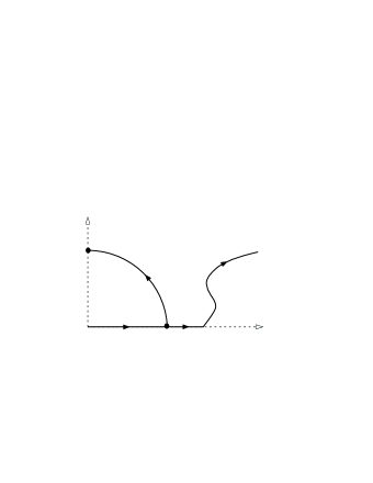
$(0,\delta)$                                    $(m_{t},n_{t})$                                                      $\sigma$                                               $\xi$          $\eta$                                                     $(\delta,0)$

Figure 2: The paths $\xi,\eta,$ and $\sigma$

We have paths of connections $A_{\xi}$ and $A_{\eta}$ on $X$ associated to $\xi$ and $\eta$. Here, $A_{\xi}$ is the path of connections on $X$ given by $A_{t}$ for $0\leq t\leq\delta$, and $A_{\eta}$ is the path of connections on $X$ given by $A_{t}$ for $\delta\leq t\leq 1.$ In addition, using the construction of Subsection 3.3, we can associate to $\sigma$ a path of connections $A_{\sigma}$ on $Y$ using the formula

$$A_{\sigma}(t)=-q(r)\delta\cos(t)idx-\delta\sin(t)idy,\quad t\in[0,\tfrac{\pi}{2}].$$

Theorem 3.9.

Given a path $A_{t}$ of connections satisfying conditions 1–3 of Subsection 3.4, consider the paths $\xi,\eta,$ and $\sigma$ defined above and the associated paths of connections $A_{\xi}(t),A_{\eta}(t),$ and $A_{\sigma}(t)$. Denote by $\bar{\sigma}\cdot\eta$ the path from $(0,\delta)$ to $(m_{1},n_{1})$ which traces $\sigma$ backwards and then follows $\eta$, and denote by $A_{\bar{\sigma}\cdot\eta}$ the corresponding path of connections on $Y$. The spectral flow of $D_{A_{t}}$ on $X$ splits according to the decomposition $X=Y\cup_{T}Z$ as

$$SF(A_{t};X)=SF(A_{\bar{\sigma}\cdot\eta}(t);Y;P^{+})+SF(A_{\eta}(t);Z;P^{-})-2.$$ (3.7)

The proof of Theorem 3.9 is somewhat difficult and has been relegated to the next subsection. The impatient reader is invited to skip ahead.

Section 4 contains a general computation of spectral flow on the solid torus. Regarding the other term, there are effective methods for computing the spectral flow on the knot complement when the restriction of $A_{t}$ to $Z$ is flat for all $t$ (see [16, 20, 21, 22, 24]). For example, the main result of [16] shows that after a homotopy of $A_{\eta}(t)$ rel endpoints, one can assume that the paths $m_{t}$ and $n_{t}$ are piecewise analytic. The results of [21], combined with those of [22], can then be used to determine $SF(A_{\eta}(t);Z;P^{-})$. The essential point is that the spectral flow along a path of flat connections on $Z$ is a homotopy invariant calculable in terms of Massey products on the twisted cohomology of $Z$.

3.7 Proof of Theorem 3.9

Applying Theorem 2.16 shows that the spectral flow is given by the Maslov index, ie, that

$$SF(A_{t};X)=\operatorname{Mas}(\Lambda_{Y}(t),\Lambda_{Z}(t)).$$

Since the Maslov index is additive with respect to composition of paths and is invariant under homotopy rel endpoints, we prove (3.7) by decomposing $\Lambda_{Y}(t)$ and $\Lambda_{Z}(t)$ into 14 paths. That is, we define paths $M_{i}$ and $N_{i}$ of Lagrangians for $i=1,\ldots,14$ so that $\Lambda_{Y}(t)$ and $\Lambda_{Z}(t)$ are homotopic to the composite paths $M_{1}\cdots M_{14}$ and $N_{1}\cdots N_{14},$ respectively. We will then use the results of the previous section to identify $\operatorname{Mas}(M_{i},N_{i})$ for $i=1,\ldots,14$. The situation is not as difficult as it first appears, as most of the terms vanish. Nevertheless, introducing all the terms helps separate the contributions of $Y$ and $Z$ to the spectral flow.

Let $a_{\xi},a_{\eta}$ and $a_{\sigma}$ denote the paths of connections on $T$ obtained by restricting $A_{\xi},A_{\eta}$ and $A_{\sigma}.$ In order to define $M_{i}$ and $N_{i},$ we need to choose a path ${\mathcal{L}}_{t}$ of finite-dimensional Lagrangians in $\ker S_{\theta}$ with the property that ${\mathcal{L}}_{0}=L_{Z}$ and ${\mathcal{L}}_{1}=K^{+}_{0}$. A specific path ${\mathcal{L}}_{t}$ will be given later, but it should be emphasized that the end result is independent of that particular choice.

We are ready to define the 14 paths $(M_{i},N_{i})$ of pairs of infinite-dimensional Lagrangians. In each case Lemma 2.18 shows these to be Fredholm pairs, so that their Maslov indices are defined.

1. Let $M_{1}$ be the constant path at the Lagrangian $\Lambda_{Y}(0)$ and $N_{1}$ be the path which stretches $\Lambda^{R}_{Z}$ to its adiabatic limit. Thus, using Corollary 3.5, we have

   $$N_{1}(t)=\begin{cases}\Lambda^{1/(1-t)}_{Z}(0)&\text{if $0\leq t<1$},\\ L_{Z}\oplus P^{+}_{\theta}&\text{if $t=1$}.\end{cases}$$

   Theorem 2.7 shows that $N_{1}$ is continuous and it follows from Lemma 2.18 that $(M_{1}(t),N_{1}(t)$ form a Fredholm pair for all $t$.

   Since $\Lambda_{Y}(0)\cap\Lambda^{R}_{Z}(0)\cong H^{0+1}(X;{\mathbb{C}}^{2})$ is independent of the length of the collar $R$, it follows that $\dim(M_{1}(t)\cap N_{1}(t))=2$ for $0\leq t<1$. At $t=1$, we have

   $$M_{1}(1)\cap N_{1}(1)=\Lambda_{Y}\cap(L_{Z}\oplus P^{+}_{\theta})=L_{Y}\cap L_{Z}$$

   by Proposition 2.10, since $H^{1}(Y,T;{\mathbb{C}}^{2})=0$. Since $\dim(L_{Y}\cap L_{Z})=2$, it follows by Proposition 2.14 that $\operatorname{Mas}(M_{1},N_{1})=0.$

2. Let $M_{2}$ be the constant path at the Lagrangian $\Lambda_{Y}(0)$. Let $N_{2}(t)={\mathcal{L}}_{t}\oplus P^{+}_{\theta}.$ We claim that $\operatorname{Mas}(M_{2},N_{2})=\operatorname{Mas}(L_{Y},{\mathcal{L}}_{t}).$

   To see this, notice that $M_{2}$ is homotopic rel endpoints to the composite of 3 paths, the first stretches $\Lambda_{Y}(0)$ to its adiabatic limit $P_{\theta}^{-}\oplus L_{Y}$, the second is the constant path at $P_{\theta}^{-}\oplus L_{Y}$, and the third is the reverse of the first, starting at the adiabatic limit $P_{\theta}^{-}\oplus L_{Y}$ and returning to $\Lambda_{Y}(0)$.

   The path $N_{2}$ is homotopic rel endpoints to the composite of 3 paths, the first is constant at ${\mathcal{L}}_{0}\oplus P_{\theta}^{+}$, the second is ${\mathcal{L}}_{t}\oplus P_{\theta}^{+}$, and the third is constant at ${\mathcal{L}}_{1}\oplus P_{\theta}^{+}$.

   Using homotopy invariance and additivity of the Maslov index, we can write $\operatorname{Mas}(M_{2},N_{2})$ as a sum of three terms. The first term is zero since $\Lambda_{Y}^{R}(0)\cap({\mathcal{L}}_{0}\oplus P_{\theta}^{+})$ has dimension equal to $\dim(L_{Y}\cap{\mathcal{L}}_{0})$ for all $R$ by Proposition 2.10, and this also equals the dimension of

   $$(\lim_{R\to\infty}\Lambda^{R}_{Y}(0))\cap({\mathcal{L}}_{0}\oplus P_{\theta}^{+})=(P_{\theta}^{-}\oplus L_{Y})\cap({\mathcal{L}}_{0}\oplus P_{\theta}^{+}).$$

   Since the dimension of the intersections is constant, the Maslov index vanishes. Similarly the third term is zero. This leaves the second term, which equals

   $$\operatorname{Mas}(P_{\theta}^{-}\oplus L_{Y},{\mathcal{L}}_{t}\oplus P_{\theta}^{+})=\operatorname{Mas}(L_{Y},{\mathcal{L}}_{t}).$$

3. Let $M_{3}$ be the path $\Lambda_{Y}(t)$ for $0\leq t\leq\delta\$ (this is the path of Lagrangians associated to $A_{\xi}$ on $Y$). Let

   $$N_{3}(t)=\begin{cases}K^{+}_{0}\oplus P^{+}_{\theta}&\hbox{ if }t=0\\ P^{+}_{a_{\xi}(t)}&\hbox{ if }0<t\leq 1.\\ \end{cases}$$

   That $N_{3}$ is continuous in $t$ was shown in the previous subsection.

4. Let $M_{4}$ be the path $\Lambda_{Y,A_{\sigma}(t)}$ and $N_{4}$ the path $P^{+}_{a_{\sigma}(t)}.$

Lemma 3.10.

$\operatorname{Mas}(M_{3}\cdot M_{4},N_{3}\cdot N_{4})=\operatorname{Mas}(L_{Y},K^{+}_{t\pi/2})$.

ProofLet $\zeta$ be the vertical line from $(0,0)$ to $(0,\delta)$ and observe that the path $\xi\cdot\sigma$ is homotopic to $\zeta$. Denote by $A_{\zeta}(t)$ the associated path of flat connections on $Y$ with connection 1–form given by $-t\delta\,idy$ (this is just the path $A_{0,t\delta})$. Then $M_{3}\cdot M_{4}$ is homotopic rel endpoints to $M_{3}^{\prime}\cdot M_{4}^{\prime},$ where $M_{3}^{\prime}$ is the constant path $\Lambda_{Y}(0)$ and $M_{4}^{\prime}(t)=\Lambda_{Y,A_{\zeta}(t)}$. Similarly, $N_{3}\cdot N_{4}$ is homotopic to $N_{3}^{\prime}\cdot N_{4}^{\prime}$, where

$$N_{3}^{\prime}(t)=K^{+}_{{t\pi}/{2}}\oplus P^{+}_{\theta},$$

$$N_{4}^{\prime}(t)=\begin{cases}K^{+}_{\pi/2}\oplus P^{+}_{\theta}&\text{for $t=0$}\\ P^{+}_{a_{\zeta}(t)}&\text{for $0<t\leq 1$,}\end{cases}$$

and $a_{\zeta}(t)$ denotes the restriction of $A_{\zeta}(t)$ to $T.$

Decomposing $M_{3}^{\prime}$ and $N_{3}^{\prime}$ further into three paths as in step 2 (the proof that Mas$(M_{2},N_{2})=$Mas$(L_{Y},{\mathcal{L}}_{t})$), we see that $\operatorname{Mas}(M_{3}^{\prime},N_{3}^{\prime})=\operatorname{Mas}(L_{Y},K^{+}_{t\pi/2})$.

Next, Proposition 2.10 together with the cohomology computation of Equation (3.5) shows that $M_{4}^{\prime}(0)\cap N_{4}^{\prime}(0)$ is isomorphic to $L_{Y}\cap K^{+}_{\pi/2}$, but Corollary 3.7 shows that the latter intersection is zero. Another application of Proposition 2.10 together with Equation (3.5) shows that $M_{4}^{\prime}(t)\cap N_{4}^{\prime}(t)=0$ for positive $t$. Hence $M_{4}(t)$ and $N_{4}(t)$ are transverse for all $t$ so that Mas$(M_{4}^{\prime},N_{4}^{\prime})=0$. The proof now follows from additivity of the Maslov index under composition of paths.

1. Let $(M_{5},N_{5})$ be $(M_{4},N_{4})$ run backwards, so $M_{5}(t)=\Lambda_{Y,A_{\bar{\sigma}}(t)}$ and $N_{5}(t)=P^{+}_{a_{\bar{\sigma}}(t)}$.

2. Let $M_{6}(t)=\Lambda_{Y,A_{\eta}(t)}$ and $N_{6}(t)=P^{+}_{a_{\eta}(t)}$.

Theorem 2.19 shows that

$$\operatorname{Mas}(M_{5}\cdot M_{6},N_{5}\cdot N_{6})=SF(A_{\bar{\sigma}\cdot\eta}(t);Y;P^{+}),$$ (3.8)

the advantage being that now both endpoints of $A_{\bar{\sigma}\cdot\eta}$ refer to nontrivial flat connections on $Y$. In the next section we will explicitly calculate this integer in terms of homotopy invariants of the path $\bar{\sigma}\cdot\eta$.

1. Let $M_{7}$ be the path obtained by stretching $\Lambda^{R}_{Y}(1)$ to its adiabatic limit. Since $a_{1},$ the restriction of $A_{1}$ to $T^{2},$ is a nontrivial flat connection, ${\lim_{R\to\infty}}\Lambda^{R}_{Y}(1)=P^{-}_{a_{1}}$. This follows from Corollary 3.5 applied to $Y$, or directly by combining Theorem 2.7, Proposition 2.10 and Equation (3.5).

   Let $N_{7}$ be the constant path $P^{+}_{a_{1}}$. An argument similar to the one used in step 1 shows that $\operatorname{Mas}(M_{7},N_{7})=0.$

2. Let $M_{8}(t)=P^{-}_{a_{\eta}(1-t)}$ and $N_{8}(t)=P^{+}_{a_{\eta}(1-t)}$ (this is just $N_{6}$ run backwards). Observe that since $M_{8}(t)$ and $N_{8}(t)$ are transverse for all $t$, $\operatorname{Mas}(M_{8},N_{8})=0.$

3. Let

   $$M_{9}(t)=\begin{cases}P^{-}_{a_{\xi}(1-t)}&\hbox{ if }0\leq t<1\\ K^{-}_{0}\oplus P^{-}_{\theta}&\hbox{ if }t=1\end{cases}$$

   and

   $$N_{9}(t)=\begin{cases}P^{+}_{a_{\xi}(1-t)}&\text{for $t<1$}\\ K^{+}_{0}\oplus P^{+}_{\theta}&\text{for $t=1$}.\end{cases}$$

   Now $N_{9}$ is just $N_{3}$ run backwards, and it is not difficult to see that $M_{9}(t)$ and $N_{9}(t)$ are transverse for all $t$, hence $\operatorname{Mas}(N_{9},M_{9})=0.$

4. Let $M_{10}$ be the constant path at $K^{-}_{0}\oplus P^{-}_{\theta}$ and let $N_{10}$ be $N_{2}$ run backwards, ie, $N_{2}(t)={\mathcal{L}}_{1-t}\oplus P^{+}_{\theta}.$ Thus, $\operatorname{Mas}(M_{10},N_{10})=\operatorname{Mas}(K^{-}_{0},{\mathcal{L}}_{1-t})$.

5. Let $M_{11}$ be the constant path at $K^{-}_{0}\oplus P^{-}_{\theta}$ and $N_{11}$ be $N_{1}$ run backwards, ie,

   $$N_{11}(t)=\begin{cases}L_{Z}\oplus P^{+}_{\theta}&\text{if $t=0$}\\ \Lambda^{1/t}_{Z}(0)&\text{if $t>0$.}\end{cases}$$

   Propositions 2.10 and 3.6 and Corollary 3.5 show that $M_{11}(t)$ is transverse to $N_{11}(t)$ for all $t$, hence $\operatorname{Mas}(M_{11},N_{11})=0.$

6. Let $M_{12}$ be $M_{9}$ run backwards, ie,

   $$M_{12}(t)=\begin{cases}K^{-}_{0}\oplus P^{-}_{\theta}&\hbox{ if }t=0\\ P^{-}_{a_{\xi}(t)}&\hbox{ if }0<t\leq 1.\end{cases}$$

   Let $N_{12}(t)=\Lambda_{Z,A_{\xi}(t)}$. Since the restriction of $A_{\xi}(t)$ to $Z$ is flat, Proposition 2.10 shows that $M_{12}(t)$ is transverse to $N_{12}(t)$ for all $t$. Hence $\operatorname{Mas}(M_{12},N_{12})=0.$

7. Let $M_{13}(t)=P^{-}_{a_{\eta}(t)}$ (ie, $M_{8}$ run backwards) and let $N_{13}(t)=\Lambda_{Z,A_{\eta}(t)}$. Theorem 2.19 then implies that

   $$\operatorname{Mas}(M_{13},N_{13})=SF(A_{\eta}(t);Z;P^{-}),$$

   the spectral flow on $Z$.

8. Let $M_{14}$ be $M_{7}$ run in reverse and $N_{14}$ the constant path at $\Lambda_{Z,A_{1}}$. An argument like the one in step 1 (but simpler since $\ker S_{a_{1}}=0$) shows that $M_{14}(t)\cap N_{14}(t)\cong H^{0+1}(X;{\mathbb{C}}^{2}_{A_{1}})$ for all $t$. This implies that $\operatorname{Mas}(M_{14},N_{14})=0.$

We leave it to the reader to verify that the terminal points of $M_{i}$ and $N_{i}$ agree with the initial points of $M_{i+1}$ and $N_{i+1}$ for $i=1,\ldots,13,$ and that $M_{1}\cdots M_{14}$ and $N_{1}\cdots N_{14}$ are homotopic rel endpoints to $\Lambda_{Y}(t)$ and $\Lambda_{Z}(t)$, respectively. Thus

$$SF(A_{t};M)=\operatorname{Mas}(M_{1}\cdots M_{14},N_{1}\cdots N_{14})=\sum_{i=1}^{14}\operatorname{Mas}(M_{i},N_{i}).$$

The arguments above show that $\operatorname{Mas}(M_{i},N_{i})=0$ for $i=1,7,8,9,11,12,$ and $14.$ Moreover, by Equation (3.8) and step 13, we see that

$$\operatorname{Mas}(M_{5}\cdot M_{6},N_{5}\cdot N_{6}) = SF(A_{\bar{\sigma}\cdot\eta}(t);Y;P^{+}),\hbox{ and}$$

$$\operatorname{Mas}(M_{13},N_{13}) = SF(A_{\eta}(t);Z;P^{-}).$$

To finish the proof of Theorem 3.9, it remains to show that the sum of the remaining terms

$$\operatorname{Mas}(M_{2},N_{2})+\operatorname{Mas}(M_{3}\cdot M_{4},N_{3}\cdot N_{4})+\operatorname{Mas}(M_{10},N_{10})$$

equals $-2$. By Step 2, Lemma 3.10, and Step 10, these summands equal $\operatorname{Mas}(L_{Y},{\mathcal{L}}_{t})$, $\operatorname{Mas}(L_{Y},K^{+}_{t\pi/2})$ and $\operatorname{Mas}(K^{-}_{0},{\mathcal{L}}_{1-t})$, respectively.

Define the path ${\mathcal{L}}_{t}$ to be

$${\mathcal{L}}_{t} = \operatorname{span}\{(1,\ (1-t)idx+tidy,0)\otimes e_{1},\ (1,\ (t-1)idx-tidy,0)\otimes e_{2},$$ (3.9)

$$\quad\quad\ (1-t,\ -idx,-\ tdxdy)\otimes e_{1},\ (1-t,\ idx,-\ tdxdy)\otimes e_{2}\}.$$

Lemma 3.11.

For the path ${\mathcal{L}}_{t}$ in Equation (3.9),

1. $\operatorname{Mas}(L_{Y},{\mathcal{L}}_{t})=0.$

2. $\operatorname{Mas}(L_{Y},K^{+}_{t\pi/2})=-2.$

3. $\operatorname{Mas}(K^{-}_{0},{\mathcal{L}}_{1-t})=0.$

ProofProposition 3.6 and Equation (3.9) imply that $K^{-}_{0}$ and ${\mathcal{L}}_{t}$ are transverse for $0\leq t\leq 1$. Hence $\operatorname{Mas}(K^{-}_{0},{\mathcal{L}}_{1-t})=0$. This proves claim (iii).

Next consider claim (ii). Corollary 3.7 implies that $\dim(L_{Y}\cap K^{+}_{t\pi/2})=0$ for $0<t\leq 1$. An exercise in linear algebra shows that, for small $s>0$, $\dim(e^{sJ}L_{Y}\cap K^{+}_{t\pi/2})=0$ unless $\tan(t\pi/2)=\tan(2s)$, and for this $t$ (which is positive and close to 0) the intersection has dimension 2. Apply Proposition 2.15 with $s(t)=t\pi/4$ to conclude that $\operatorname{Mas}(L_{Y},K^{+}_{t\pi/2})=-2.$

Finally, consider claim (i). It is easily verified that

$$\dim(L_{Y}\cap{\mathcal{L}}_{t})=\begin{cases}2&\text{if $t=0,1$,}\\ 0&\text{if $0<t<1$.}\end{cases}$$

A direct calculation shows further that $e^{sJ}L_{Y}\cap{\mathcal{L}}_{t}\neq 0$ if and only if

$$0=(1+\sin 2s)t^{2}+(1-\sin 2s)\,t+\sin 2s,$$ (3.10)

in which case $\dim(e^{sJ}L_{Y}\cap{\mathcal{L}}_{t})=2.$ We will apply Proposition 2.15 to the intersection of $L_{Y}$ and ${\mathcal{L}}_{t}$ at $t=0$ and the ‘reversed’ result to the intersection at $t=1$ (cf. the remark immediately following the proof of Proposition 2.15). The solutions $t=t(s)$ to (3.10) are the two functions

$$t_{\pm}(s)=\frac{1}{2}\pm\frac{1}{2}\sqrt{\frac{1+3\sin 2s}{1-\sin 2s}}.$$

Notice that $t_{+}(0)=1$ and $t^{\prime}_{+}(0)>0$ and $t_{-}(0)=0$ and $t_{-}^{\prime}(0)<0.$ Apply Proposition 2.15 to $s_{-}(t)$ at $t=0$, and also apply its reversed result to $s_{+}(t)$ at $t=1$, where $s_{\pm}$ denote the inverse functions of $t_{\pm}$. It follows that $\operatorname{Mas}(L_{Y},{\mathcal{L}}_{t};\ 0\leq t\leq\delta)=0$ and $\operatorname{Mas}(L_{Y},{\mathcal{L}}_{t};\ 1-\delta\leq t\leq 1)=0.$

4 Spectral flow on the solid torus

In this section, we carry out a detailed analysis of connections on the solid torus $Y$ and show how to compute the spectral flow between two nontrivial flat connections on $Y$. We reduce the computation to an algebraic problem by explicitly constructing the Cayley graph associated to the gauge group using paths of connections.

4.1 An SU(2) gauge group for connections on Y in normal form on T

We begin by specifying certain groups of gauge transformations which leave invariant the spaces of connections on $T$ and $Y$ which are in normal form (on $T$ or along the collar). We will identify $SU(2)$ with the 3–sphere $S^{3}$ of unit quaternions, and we identify the diagonal subgroup with $S^{1}\subset S^{3}$.

Define $\tilde{\alpha},\tilde{\beta}\co T\to S^{1}$ by the formulas

$$\tilde{\alpha}(e^{ix},e^{iy})=e^{ix},\ \ \tilde{\beta}(e^{ix},e^{iy})=e^{iy}.$$

Let $H$ be the abelian group generated by $\tilde{\alpha}$ and $\tilde{\beta}$, which act on ${\mathcal{A}}_{\rm nf}(T)$ by

$$\tilde{\alpha}\cdot a_{m,n}=a_{m+1,n},\ \ \tilde{\beta}\cdot a_{m,n}=a_{m,n+1}.$$

Let ${\mathcal{A}}_{\rm nf}(Y)$ denote the space of connections on $Y$ which are in normal form on the collar (cf. Definition 3.1),

$${\mathcal{A}}_{\rm nf}(Y)=\{A\in\Omega^{1}_{Y}\otimes su(2)\mid A|_{[-1,0]\times T}\text{ is cylindrical and in normal form}\}.$$

Let $r\co{\mathcal{A}}_{\rm nf}(Y)\to{\mathcal{A}}_{\rm nf}(T)$ denote the restriction map. We define the gauge group

$${\mathcal{G}}_{\rm nf}=\{\text{smooth maps }g\co Y\to S^{3}\mid g|_{[-1,0]\times T}=\pi^{*}h\text{ for some }h\in H\},$$

where $\pi\co[-1,0]\times T\to T$ is projection. It is clear that, for $g\in{\mathcal{G}}_{\rm nf}$ with $g|_{T}=h$, we have the commutative diagram

$$\begin{CD}{\mathcal{A}}_{\rm nf}(Y)@>{g}>{}>{\mathcal{A}}_{\rm nf}(Y)\\ @V{r}V{}V@V{}V{r}V\\ {\mathcal{A}}_{\rm nf}(T)@>{}>{h}>{\mathcal{A}}_{\rm nf}(T).\\ \end{CD}$$

To clarify certain arguments about homotopy classes of paths, it is convenient to replace the map $r\co{\mathcal{A}}_{\rm nf}(Y)\to{\mathcal{A}}_{\rm nf}(T)$ with the map $Q\co{\mathcal{A}}_{\rm nf}(Y)\to{\mathbb{R}}^{2}$ defined by

$$Q(A)=(m,n)\text{ where }A|_{T}=a_{m,n}.$$

The identity component ${\mathcal{G}}_{\rm nf}^{0}\subset{\mathcal{G}}_{\rm nf}$ is a normal subgroup, and we denote the quotient by $G={\mathcal{G}}_{\rm nf}/{\mathcal{G}}_{\rm nf}^{0}$.

Recalling the orientation on $Y$ from Section 3.1 and using the orientation of $S^{3}$ given by the basis $\{i,j,k\}$ for $T_{1}S^{3}$, we note that each $g\in{\mathcal{G}}$ has a well-defined degree, since $H_{3}(S^{3},S^{1};{\mathbb{Z}})={\mathbb{Z}}$, and this degree remains well-defined on $G$.

Lemma 4.1.

Let $g,g^{\prime}\in{\mathcal{G}}_{\rm nf}$. Then $g$ is homotopic to $g^{\prime}$ (ie, they represent the same element of $G$) if and only if $(g|_{T})=(g^{\prime}|_{T})$ and $\deg(g)=\deg(h)$.

ProofThis is a simple application of obstruction theory that we leave to the reader.

It follows from Lemma 4.1 that the restriction map descends to a map $P\co G\to H$ which is onto, since $\pi_{1}(S^{3})=\pi_{2}(S^{3})=0$. Set $K=\ker P\cong{\mathbb{Z}}$, where the last isomorphism is given by the degree.

Lemma 4.2.

The kernel of $P\co G\to H$ is central.

ProofSuppose $k\in K$ and $g\in G$. After a homotopy, we may assume that there is a 3–ball $B^{3}$ contained in the interior of $Y$ such that $k|_{Y-B^{3}}=1$ and $g|_{B^{3}}=1$. It follows directly from this that $gk=kg$.

Using the cutoff function $q(r)$ from Equation (3.6), we define $\alpha,\beta,\gamma\in G$ as follows (we make the definitions in ${\mathcal{G}}_{\rm nf}$ but they should be reduced mod ${\mathcal{G}}^{0}_{\rm nf}$):

1. $\alpha(re^{ix},w)=q(r)e^{ix}+\sqrt{1-(q(r))^{2}}j.$

2. $\beta(re^{ix},w)=w$,

3. $\gamma(z,w)=\hbox{ a generator of }K\hbox{ with }\deg(\gamma)=1.$

It will be useful to denote by $\bar{\alpha}$ the map

$$\bar{\alpha}(re^{ix},w)=re^{ix}+\sqrt{1-r^{2}}j,$$

which is not in ${\mathcal{G}}_{\rm nf}$ but is homotopic rel boundary to $\alpha$ and has a simpler formula. Using $\bar{\alpha}$ will simplify the computation of degrees of maps involving $\alpha$. Observe that

$$\begin{array}[]{lll}P(\alpha)=\tilde{\alpha}&\hbox{and}&\deg(\alpha)=0\\ P(\beta)=\tilde{\beta}&\hbox{and}&\deg(\beta)=0\\ P(\gamma)=1&\hbox{and}&\deg(\gamma)=1.\end{array}$$

Now $[\alpha,\gamma]=[\beta,\gamma]=1$, hence $G$ is a central extension of $H$ by $K$:

$$0\longrightarrow K\longrightarrow G\longrightarrow H\longrightarrow 0.$$

Such extensions are classified by elements of $H^{1}(H;{\mathbb{Z}}),$ and to determine the cocycle corresponding to our extension, we just need to calculate which element of $K$ is represented by the map $[\alpha,\beta]$. This amounts to calculating the degree of this map.

Lemma 4.3.

$[\alpha,\beta]=\gamma^{-2}$.

ProofSet $h=[\alpha,\beta].$ Clearly, $h\in\ker(P)$, so we just need to calculate its degree. It is sufficient to compute the degree of $\bar{h}=[\bar{\alpha},\beta]$, since it is homotopic to $h$ rel boundary. Using the coordinates $(re^{ix},e^{iy})$ for $Y$ and writing quaternions as $A+jB$ for $A,B\in{\mathbb{C}},$ we compute that

$$\bar{h}(re^{ix},e^{iy})=r^{2}+(1-r^{2})e^{-2iy}+jr\sqrt{1-r^{2}}e^{-ix}(1-e^{-2iy}).$$

To determine the degree of $\bar{h}$, consider the value $k\in S^{3}$ which we will prove is a regular value. Solving $\bar{h}(re^{ix},e^{iy})=k$ yields the two solutions $r={\frac{1}{\sqrt{2}}}$, $x={\frac{\pi}{2}}$, $y={\frac{\pi}{2}}\hbox{ or }{\frac{3\pi}{2}}$. Applying the differential $d\bar{h}$ to the oriented basis $\{\frac{\partial}{\partial r},{\frac{\partial}{\partial x}},{\frac{\partial}{\partial y}}\}$ for the tangent space of $Y$ and then translating back to $T_{1}(S^{3})$ by right multiplying by $-k$ gives the basis $\{-2\sqrt{2}k,i,i+j\}$ of $S^{3}$, which is negatively oriented compared to $\{i,j,k\}$. Since the computation gives this answer for both inverse images of $k$, it follows that $\deg(h)=-2$, which proves the claim.

We have now established the structure of $G$. Every element $g\in G$ can be expressed uniquely as $g=\alpha^{a}\beta^{b}\gamma^{c}$ where $a,b,c\in{\mathbb{Z}}$. Furthermore, with respect to this normal form, multiplication can be computed as follows:

$$(\alpha^{a_{1}}\beta^{b_{1}}\gamma^{c_{1}})(\alpha^{a_{2}}\beta^{b_{2}}\gamma^{c_{2}})=\alpha^{a_{1}+a_{2}}\beta^{b_{1}+b_{2}}\gamma^{2b_{1}a_{2}+c_{1}+c_{2}}$$

The next result determines the degree of any element in normal form.

Theorem 4.4.

$\deg(\alpha^{a}\beta^{b}\gamma^{c})=c-ab$.

ProofWe begin by computing the degree of $\alpha^{a}\beta^{b}$. Let $f_{a}\co D^{2}\times S^{1}\to S^{3}$ be the map

$$f_{a}(re^{ix},e^{iy})=\alpha(r^{|a|}e^{iax},e^{iby})=r^{|a|}e^{iax}+\sqrt{1-r^{2|a|}}j.$$

Then $f_{a}$ is homotopic rel boundary to $\bar{\alpha}^{a}$ using Lemma 4.1 since they agree on the boundary and both have degree $0$ (they factor through the projection to $D^{2}$).

The degree of $\alpha^{a}\cdot\beta^{b}$ equals the degree of $f_{a}\cdot\beta^{b}$, since $\alpha^{a}$ is homotopic to $f_{a}$.

But $f_{a}\cdot\beta^{b}$ factors as the composite of the map

$$D^{2}\times S^{1}\longrightarrow D^{2}\times S^{1}$$

$$(re^{ix},e^{iy})\mapsto(r^{|a|}e^{iax},e^{iby})$$

and the map

$$D^{2}\times S^{1}\longrightarrow S^{3}$$

$$(z,w)\mapsto\bar{\alpha}(z,w)\beta(z,w).$$

The first map is a product of a branched cover of degree $a$ and a cover of degree $b$ and so has degree $ab$. The second restricts to a homeomorphism of the interior of the solid torus with $S^{3}-S^{1}$ which can easily be computed to have degree $-1$. Thus $\alpha^{a}\beta^{b}$ has degree $-ab$.

To finish proving the theorem, we need to calculate the effect of multiplying by $\gamma$. For any $g\in{\mathcal{G}}$, we can arrange by homotopy that $\gamma$ is supported in a small 3-ball while $g$ is constant in the same 3-ball. It is then clear that for all $g\in G$, $\deg(g\gamma)=\deg(g)+1$.

4.2 The ${{\mathbb{C}}^{2}}$–spectral flow on Y

Suppose that $A_{t}\in{\mathcal{A}}_{\rm nf}(Y)$ is a path between the flat connections $A_{0}$ and $A_{1}$ on $Y$. We will present a technique for computing $SF(A_{t};Y;P^{+}),$ the spectral flow of the odd signature operator

$$D_{A_{t}}\co\Omega^{0+1}_{Y}\otimes{\mathbb{C}}^{2}\longrightarrow\Omega^{0+1}_{Y}\otimes{\mathbb{C}}^{2}$$

on $Y$ with $P^{+}$ boundary conditions. We assume that for all $t$, $Q(A_{t})\in{\mathbb{R}}^{2}-{\mathbb{Z}}^{2}$. This implies that $P^{+}_{a_{t}}$ varies continuously in $t,$ where $a_{t}$ denotes the restriction of $A_{t}$ to $T$ [23]. Moreover the exact sequence in Proposition 2.10 shows that the kernels of $D_{A_{0}}$ and $D_{A_{1}}$ with $P^{+}$ boundary conditions are zero.

Lemma 4.5.

Let $Y_{1}$ and $Y_{2}$ be solid tori, and let $X=Y_{1}\cup Y_{2}$ be the lens space obtained by gluing $\partial Y_{1}$ to $\partial Y_{2}$ using an orientation reversing isometry $h\co\partial Y_{1}\to\partial Y_{2}$. Let $A_{t}$ be a path in ${\mathcal{A}}_{\rm nf}(Y_{1})$ and $B_{t}$ a path in ${\mathcal{A}}_{\rm nf}(Y_{2})$ so that $h^{*}(B_{t}|_{\partial Y_{2}})=A_{t}|_{\partial Y_{1}}$. Assume that $Q(A_{t})\in{\mathbb{R}}^{2}-{\mathbb{Z}}^{2}$ and that $A_{0},A_{1},B_{0},B_{1}$ are flat. Then

$$SF(A_{t}\cup B_{t};X)=SF(A_{t};Y_{1};P^{+})+SF(B_{t};Y_{2};P^{+}).$$

ProofWrite $T=\partial Y_{1}$ and let $a_{t}=A_{t}|_{T}$. The cohomology computation (3.4) shows that $H^{0+1+2}(T;{\mathbb{C}}^{2}_{a_{t}})=0$ for all $t$. Hence $\ker S_{a_{t}}=0$ for all $t$. Also, the computation (3.5) shows that $H^{0+1}(Y_{1};{\mathbb{C}}^{2}_{A_{i}})=\ker D_{A_{i}}(P^{+})=0$ for $i=0,1$ and that $H^{0+1}(Y_{1};{\mathbb{C}}^{2}_{B_{i}})=\ker D_{B_{i}}(P^{+})=0$ for $i=0,1.$

The lemma now follows from the splitting theorem for spectral flow of Bunke (Corollary 1.25 of [7]). For a simple proof using the methods of this article see [14].

Lemma 4.6.

Suppose $A_{t}$ and $B_{t}$ are two paths in ${\mathcal{A}}_{\rm nf}(Y)$ such that $A_{i}$ and $B_{i}$ are flat for $i=0,1$. Suppose further that the paths $Q(A_{t})$ and $Q(B_{t})$ miss the integer lattice ${\mathbb{Z}}^{2}\subset{\mathbb{R}}^{2}$ for all $t\in[0,1].$ If $A_{i}=g_{i}\cdot B_{i}$ for $i=0,1$ where $g_{i}\in{\mathcal{G}}_{\rm nf}^{0}$ and if the paths $Q(A_{t})$ and $Q(B_{t})$ are homotopic rel endpoints in ${\mathbb{R}}^{2}-{\mathbb{Z}}^{2}$, then $SF(A_{t};Y;P^{+})=SF(B_{t};Y;P^{+})$.

ProofFirst, note that a path of the form $g_{t}A$, where $g_{t}$ is a path in ${\mathcal{G}}$, has spectral flow zero, because the eigenvalues are all constant. (This follows from the fact that the operators in the path are all conjugate.) Hence we may assume that $A_{i}=B_{i}$ for $i=0,1$ (if not, add a path of the form $g_{t}A_{i}$ to each end of $B_{t}$ bringing the endpoints together). Now, using the fact that ${\mathcal{A}}_{\rm nf}(Y)$ is a bundle over ${\mathcal{A}}_{\rm nf}(T)$ with contractible fiber, it is easy to see that the homotopy between $Q(A_{t})$ and $Q(B_{t})$ can be lifted to one between $A_{t}$ and $B_{t}$ which will, of course, avoid $Q^{-1}({\mathbb{Z}}^{2})$. Finally, homotopic paths of operators have the same spectral flow, proving the lemma.

Based on this lemma, we may now state precisely the question we wish to answer: Given a path of connections $A_{t}$ in ${\mathcal{A}}_{\rm nf}(Y)$ between two flat connections such that $Q(A_{t})$ avoids ${\mathbb{Z}}^{2}\subset{\mathbb{R}}^{2}$, how can one calculate $SF(A_{t};Y;P^{+})$ from $A_{0}$, $A_{1}$, and the image $Q(A_{t})$ in ${\mathbb{R}}^{2}-{\mathbb{Z}}^{2}$?

The following lemmas serve as our basic computational tools in what follows.

Lemma 4.7.

Suppose $X$ is a closed oriented 3–manifold and $g\co X\to SU(2)$ is a gauge transformation. If $A_{0}$ is any $SU(2)$ connection on $X$, and $A_{t}$ is any path of connections from $A_{0}$ to $A_{1}=g\cdot A_{0}=gA_{0}g^{-1}-dg~{}g^{-1}$, then

$$SF({A_{t}};X)=-2\deg(g).$$

ProofRecall that we are using the $(-\varepsilon,-\varepsilon)$ convention for computing spectral flows. The claim follows from a standard application of the Index Theorem. See for example the appendix to [24].

Lemma 4.8.

Let $A$ be any connection in ${\mathcal{A}}_{\rm nf}(Y)$ with $Q(A)\in{\mathbb{R}}^{2}-{\mathbb{Z}}^{2}$ and let $g\in{\mathcal{G}}_{\rm nf}$ be a gauge transformation which is $1$ on the collar neighborhood of the boundary $T$. If $A_{t}$ is any path in ${\mathcal{A}}_{\rm nf}(Y)$ from $A$ to $g\cdot A$ which is constant on $T$ (eg, the straight line from $A$ to $g\cdot A$), then $SF(A_{t};Y;P^{+})=-2\deg(g)$.

ProofConsider a path $B_{t}$ of connections on the double $D(Y)$ of $Y$ which is constant at $A$ on one side and is $A_{t}$ on the other side, and the gauge transformation $h$ which is $g$ on one side and the identity on the other. Then $B_{1}=hB_{0}$, and $\deg(h)=\deg(g)$. Lemma 4.7 shows that $SF(B_{t};D(Y))=-2\deg(g)$. Now apply Lemma 4.5.

Since we are interested in paths between flat connections, we begin by analyzing the components of orbits of flat connections in ${\mathcal{A}}_{\rm nf}(Y)/{\mathcal{G}}_{\rm nf}^{0}$. First, note that all the flat connections in ${\mathcal{A}}_{\rm nf}(Y)$ project to ${\mathbb{Z}}\times{\mathbb{R}}$ under $Q\co{\mathcal{A}}_{\rm nf}(Y)\to{\mathbb{R}}^{2}$. Set $\tilde{J}$ equal to the open vertical line segment $\tilde{J}=\{(0,t)\mid 0<t<1\}\subset{\mathbb{R}}^{2}$.

A natural choice of gauge representatives for $Q^{-1}(\tilde{J})$ is the path of connections $J=\{-tidy\mid 0<t<1\}\subset{\mathcal{A}}_{\rm nf}(Y)$. The connection $-tidy$ is a flat connection on $Y$ whose holonomy sends $\mu$ to $1$ and $\lambda$ to $e^{2\pi it}$. Note that the spectral flow of any path $A_{t}$ whose image modulo ${\mathcal{G}}_{\rm nf}^{0}$ lies in $J$ is 0, since $\ker D_{A_{t}}$ is constantly zero.

The set of all flat orbits in ${\mathcal{A}}_{\rm nf}(Y)/{\mathcal{G}}_{\rm nf}^{0}$ not containing any gauge transformations of the trivial connection may be expressed as $\bigcup_{g\in G}(g\cdot J)$. For every nontrivial $g\in G$, $g\cdot J$ is disjoint from $J$. This can be seen by considering the action of $P(g)$ on $J$, and using Lemma 4.8 above. The reader is encouraged to visualize the orbit of $J$ under $G$ as consisting of ${\mathbb{Z}}$ homeomorphic copies of $J$ sitting above each translate $(p,q)+\tilde{J}$ in ${\mathbb{R}}^{2}$, where $p$ and $q$ are integers.

We will now build a graph $\Gamma$ with one vertex corresponding to each component of $G\cdot J$. Note that these vertices are also in one-to-one correspondence with $G$. Next, we will construct some directed edges with $J$ as their initial point. Actually, for specificity, we will think of their initial point as being $c_{0}=-{\tfrac{1}{2}}idy$ of $J$.

Let $E_{\alpha}$ be the straight line path of connections from $c_{0}$ to $\alpha\cdot c_{0}$. We construct a corresponding (abstract) edge in $\Gamma$ from $J$ to $\alpha J$, which we also denote by $E_{\alpha}$. Now for all $g\in G$, construct another edge $gE_{\alpha}$ from $g\cdot J$ to $g\alpha J$, which one should think of as corresponding to the path $gE_{\alpha}$ in ${\mathcal{A}}_{\rm nf}(Y)$. Thus every vertex of $\Gamma$ serves as the initial point of one $\alpha$–edge and the terminal point of another.

Next we construct a path $E_{\beta}$ in ${\mathcal{A}}_{\rm nf}(Y)$ from $c_{0}$ to $\beta c_{0}$. We cannot use the straight line because its image in ${\mathbb{R}}^{2}$ hits the integer lattice, so instead we define $E_{\beta}$ to be the path in ${\mathcal{A}}_{\rm nf}(Y)$ given by

$$A_{t}=-\tfrac{1}{2}q(r)\cos t\ idx-(1+\tfrac{1}{2}\sin t)\ idy,\ \ -\tfrac{\pi}{2}\leq t\leq\tfrac{\pi}{2},$$

where $q(r)$ is the radial bump function in Equation (3.6). Thus $Q(E_{\beta})$ is the semicircle $(\tfrac{1}{2}\cos t,1+\tfrac{1}{2}\sin t)$, $t\in[-\tfrac{\pi}{2},\tfrac{\pi}{2}]$. (As before, it is only the homotopy class of the path $E_{\beta}$ in $Q^{-1}({\mathbb{R}}^{2}-{\mathbb{Z}}^{2})$ rel endpoints that is important.) For each $g\in G$, build an edge $gE_{\beta}$ in $\Gamma$ from $g\cdot J$ to $g\beta\cdot J$ corresponding to the path of connections $gE_{\beta}$.

Finally, construct a path of connections $E_{\gamma}$ in ${\mathcal{A}}_{\rm nf}(Y)$ from $c_{0}$ to $\gamma c_{0}$ such that $Q(E_{\gamma})$ is the constant path in ${\mathbb{R}}^{2}$ at $(0,\frac{1}{2})$. A straight-line path would be acceptable in this case. Once again, for each $g\in G$, define an edge $gE_{\gamma}$ in $\Gamma$ from $g\tilde{J}$ to $g\gamma\tilde{J}$. The resulting graph $\Gamma$ is isomorphic to the Cayley graph of $G$, defined with respect to right multiplication by the generators $\{\alpha,\beta,\gamma\}$.

Notice that we have also constructed a 1–dimensional graph in ${\mathcal{A}}_{\rm nf}(Y)$ the image of which in ${\mathcal{A}}_{\rm nf}(Y)/{\mathcal{G}}_{\rm nf}^{0}$ is invariant under $G$; this will provide us with a complete (up to homotopy and gauge transformation in ${\mathcal{G}}_{\rm nf}^{0}$) collection of paths of connections in ${\mathcal{A}}_{\rm nf}(Y)$ connecting components of the flat connections in $Q^{-1}({\mathbb{R}}^{2}-{\mathbb{Z}}^{2})$.

The next step is to associate to each edge of $\Gamma$ an integer, which will give the spectral flow of the odd signature operator $D_{A}$ on the solid torus $Y$ with $P^{+}$ boundary conditions along the corresponding path of connections in ${\mathcal{A}}_{\rm nf}(T)$. Of course, the integer associated to the path $gE_{\alpha}$ is independent of $g\in G$ since the gauge transformation $g$ induces a relation of conjugacy between $D_{A}$ and $D_{g\cdot A}$ for each $A$ in the path. An analogous fact holds for the edges $E_{\beta}$ and $E_{\gamma}$, as well. So we just need to find three integers $k_{\alpha}$, $k_{\beta}$, and $k_{\gamma}$, one for each class of edges.

Theorem 4.9.

These constants have values $k_{\alpha}=2$, $k_{\beta}=-2$, and $k_{\gamma}=-2$.

ProofThe value of $k_{\gamma}$ is calculated to be $-2$ in Lemma 4.8, so we turn our attention to calculating $k_{\alpha}$ and $k_{\beta}$.

Let $Y_{1}$ and $Y_{2}$ be two solid tori with the same orientations. For $i=1,2,$ set $T_{i}=\partial Y_{i}$ with coordinates $x_{i},y_{i}$ and let $\mu_{i}$, $\lambda_{i}$, $dx_{i}$, and $dy_{i}$ denote the loops and forms on $Y_{i}$. Glue $Y_{1}$ to $Y_{2}$ by the homeomorphism of $T_{1}$ with $T_{2}$ which identifies $(e^{ix_{1}},e^{iy_{1}})$ with $(e^{i(x_{2}+y_{2})},e^{i(2x_{2}+y_{2})})$. Since this map is orientation reversing, we may give $Y_{1}\cup Y_{2}$ the orientation of both $Y_{1}$ and $Y_{2}$. Let $A_{1,t}$ denote the path of connections on $Y_{1}$ corresponding to $E_{\alpha}$. When restricted to $T_{1}$, these connections are given by the straight line, ie, $A_{1,t}|_{T_{1}}=-tidx_{1}-\frac{1}{2}idy_{1}$.

We now need to construct a path of connections on $Y_{2}$ which is compatible along $T_{2}$ with $A_{1,t}|_{T}$. Pulling the connections $A_{1,t}|_{T_{1}}$ back to $T_{2}$ by the above formula gives a path

$$a_{t}=-(t+1)idx_{2}-(t+\frac{1}{2})idy_{2}$$

of connections on $T_{2}$. Under the identification ${\mathcal{A}}_{\rm nf}(T_{2})\cong{\mathbb{R}}^{2}$, this is the straight line from $(1,\frac{1}{2})$ to $(2,\frac{3}{2})$. Now define the path $B_{t}$ in ${\mathcal{A}}_{\rm nf}(Y_{2})$ by first following the path $\alpha E_{\beta}$ from $\alpha c_{0}$ to $\alpha\beta c_{0}$, and then the path $\alpha\beta E_{\alpha}$ from $\alpha\beta c_{0}$ to $\alpha\beta\alpha c_{0}$. Note that $B_{t}$ runs from $\alpha c_{0}$ to $\alpha\beta\alpha c_{0}$, and that $Q(B_{t})$ is a path which is homotopic rel endpoints in ${\mathbb{R}}^{2}-{\mathbb{Z}}^{2}$ to the straight line from $(1,\frac{1}{2})$ to $(2,\frac{3}{2})$. Hence we may define a path $A_{2,t}$ in ${\mathcal{A}}_{\rm nf}(Y_{2})$ which is homotopic rel endpoints to $B_{t}$ in $Q^{-1}({\mathbb{R}}^{2}-{\mathbb{Z}}^{2})\subset{\mathcal{A}}_{\rm nf}(Y_{2})$ and has the property that $Q(A_{2,t})=(t+1,t+\frac{1}{2})$. By Lemma 4.6, $B_{t}$ and $A_{2,t}$ have the same spectral flow.

Consider the path of connections $A_{t}$ on $Y_{1}\cup Y_{2}$ defined to be $A_{1,t}$ on $Y_{1}$ and $A_{2,t}$ on $Y_{2}$. Note that $A_{1}=gA_{0}$, where $g$ is a gauge transformation on $Y_{1}\cup Y_{2}$ equal to $\alpha$ on $Y_{1}$ and equal to $\alpha\beta$ on $Y_{2}$. Since $\deg(\alpha)=0$ and $\deg(\alpha\beta)=-1$ by Theorem 4.4, it follows that $\deg(g)=-1$. Hence $SF(A_{t};Y_{1}\cup Y_{2})=2$ by Lemma 4.7. On the other hand, by Lemma 4.5,

$$SF(A_{t};Y_{1}\cup Y_{2})=SF(A_{1,t};Y_{1};P^{+})+SF(A_{2,t};Y_{2};P^{+})=2k_{\alpha}+k_{\beta}.$$

This gives the linear equation $2=2k_{\alpha}+k_{\beta}$.

Repeating this process, we glue $Y_{1}$ to $Y_{2}$ by the homeomorphism of $T_{1}$ with $T_{2}$ which identifies $(e^{ix_{1}},e^{iy_{1}})$ with $(e^{i(x_{2}+2y_{2})},e^{i(2x_{2}+3y_{2})})$. This gives another equation which can be used to solve for $k_{\alpha}$ and $k_{\beta}$. Pulling back the same path of connections $A_{1,t}|_{T_{1}}$ to $T_{2}$ using the new gluing map, we obtain

$$a_{t}=-(t+1)idx_{2}-(2t+\tfrac{3}{2})idy_{2},$$

which under the identification ${\mathcal{A}}_{\rm nf}(T_{2})\cong{\mathbb{R}}^{2}$ is the line segment from $(1,\frac{3}{2})$ to $(2,\frac{7}{2})$. We define the path $B_{t}$ in ${\mathcal{A}}_{\rm nf}(T_{2})$ by first following the path $\alpha\beta E_{\beta}$ from $\alpha\beta c_{0}$ to $\alpha\beta^{2}c_{0}$, then $\alpha\beta^{2}E_{\beta}$ from $\alpha\beta^{2}c_{0}$ to $\alpha\beta^{3}c_{0}$, then $\alpha\beta^{3}E_{\alpha}$ from $\alpha\beta^{3}c_{0}$ to $\alpha\beta^{3}\alpha c_{0}=\alpha\beta^{2}\gamma^{2}\alpha\beta c_{0}$ (the last equality is by the relation $[\alpha,\beta]=\gamma^{-2}$).

So, $B_{t}$ is a path in ${\mathcal{A}}_{\rm nf}(Y_{2})$ from $\alpha\beta c_{0}$ to $\alpha\beta^{2}\gamma^{2}(\alpha\beta c_{0})$ with the property that $Q(B_{t})$ is homotopic rel endpoints to the straight line from $(1,\frac{3}{2})$ to $(2,\frac{7}{2})$ in ${\mathbb{R}}^{2}-{\mathbb{Z}}^{2}$. Hence, as before, define a path $A_{2,t}$ in ${\mathcal{A}}_{\rm nf}(Y_{2})$ which is homotopic rel endpoints to $B_{t}$ in $Q^{-1}({\mathbb{R}}^{2}-{\mathbb{Z}}^{2})$ and has $Q(A_{2,t})=(1+t,\frac{3}{2}+2t)$. Note that $SF(A_{2,t};Y_{2};P^{+})=k_{\alpha}+2k_{\beta}$ while, as before, $SF(A_{1,t};Y_{1};P^{+})=k_{\alpha}$. Gluing together $A_{1,t}$ on $Y_{1}$ and $A_{2,t}$ on $Y_{2}$, we obtain a path $A_{t}$ of connections on $Y_{1}\cup Y_{2}$. Note that $A_{1}=gA_{0}$, where $g$ is the union of $\alpha$ on $Y_{1}$ and $\alpha\beta^{2}\gamma^{2}$ on $Y_{2}$. Since $\deg(g)=\deg(\alpha)+\deg(\alpha\beta^{2}\gamma^{2})=0$ by Theorem 4.4, it follows that $SF(A_{t};Y_{1}\cup Y_{2})=0$. On the other hand, Lemma 4.5 says

$$SF(A_{t};Y_{1}\cup Y_{2})=SF(A_{1,t};Y_{1};P^{+})+SF(A_{2,t};Y_{2};P^{+})=2k_{\alpha}+2k_{\beta},$$

which yields the equation $0=2k_{\alpha}+2k_{\beta}$.

Solving these two equations shows that $k_{\alpha}=2$ and $k_{\beta}=-2$ and completes the proof of the theorem.

5 Dehn surgery techniques for computing gauge theoretic invariants

In this section, we apply the results from Sections 3 and 4 to develop formulas for a variety of gauge theoretic invariants of flat connections on Dehn surgeries $X=Y\cup_{T}Z.$ Given a path of flat connections on $Z$ whose initial point is the trivial connection and whose terminal point extends flatly over $X$, we extend this to a path $A_{t}$ of connections on $X$ such that $A_{0}=\Theta$ and $A_{1}$ is flat. We then apply Theorem 3.9 and the results of Subsection 4.2 to derive a general formula for the ${\mathbb{C}}^{2}$–spectral flow along this path. We also give a formula for the Chern–Simons invariant of $A_{1}$ as an element in ${\mathbb{R}}$ rather than ${\mathbb{R}}/{\mathbb{Z}}$. These formulas allow computations of the spectral flow and the Chern–Simons invariants in terms of easily computed homotopy invariant quantities associated to the path $(m_{t},n_{t})\subset{\mathbb{R}}^{2}$ introduced in Subsection 3.4. To illustrate how to use the formulas in practice, we present detailed calculations for $\pm 1$ surgery on the trefoil in Subsection 5.4.

Combining the formula for the spectral flow with the one for the Chern–Simons invariant leads to a computation of the $SU(2)$ rho invariants of Atiyah, Patodi, and Singer in Subsection 5.5. Our ultimate aim is to develop methods for computing the correction term for the $SU(3)$ Casson invariant [5]. Summing the rho invariants yields the correction term provided the $SU(2)$ representation variety is regular as a subspace of the $SU(3)$ representation variety (Theorem 5.10). In Section 6, we will extend these computations to all surgeries on $(2,q)$ torus knots.

5.1 Extending paths of connections to X

Throughout this section, we denote by $A,B,C,$ and $a$ connections on $X,Y,Z$ and $T$, respectively. With respect to the manifold splitting $X=Y\cup_{T}Z,$ we have $A=B\cup_{a}C$.

Our starting point is the following. We are given a path $C_{t}$ of $SU(2)$ connections on $Z$ in normal form on the collar which are flat for $t$ near $0$ and at $t=1$ (in all the examples considered in this paper, $C_{t}$ is flat for all $t$) such that

1. $C_{0}=\Theta,$ the trivial connection on $Z.$

2. $C_{1}$ extends flatly over $X=Y\cup_{T}Z$.

3. For all $t>0$ the restriction of $C_{t}$ to the boundary torus has nontrivial holonomy.

4. For all small positive $t$, $C_{t}$ is a nontrivial reducible connection.

Let $a_{t}=C_{t}|_{T}$ be the restriction of $C_{t}$ to the boundary. Then since $C_{t}$ is in normal form, we have

$$a_{t}=-m_{t}idx-n_{t}idy$$

for $(m_{t},n_{t})\in{\mathbb{R}}^{2}.$ Conditions 1–4 imply that $(m_{0},n_{0})=(0,0)$, $m_{1}\in{\mathbb{Z}}$, $(m_{t},n_{t})\in{\mathbb{R}}^{2}-{\mathbb{Z}}^{2}$ for $t>0$, and $n_{t}=0$ for small positive $t$. Moreover, by reparameterizing $C_{t}$ and gauge transforming if necessary, we can assume that conditions 1–3 of Subsection 3.4 hold.

The path $(m_{t},n_{t})$ will usually be described starting with a path of representations. The following proposition is helpful. This proposition follows from a relative version of the main theorem of [16]. Its proof, which follows the same outline as [16], is omitted.

Proposition 5.1.

Suppose $\rho\co[0,1]\to{\rm Hom}(\pi_{1}Z,SU(2))$ is a continuous path of representations with $\rho_{t}(\mu)=e^{2\pi im_{t}}$ and $\rho_{t}(\lambda)=e^{2\pi in_{t}}$. Then there exists a path of flat connections $C_{t}$ on $Z$ in normal form such that $\operatorname{hol}_{C_{t}}=\rho_{t}$ and $C_{t}|_{T}=-m_{t}idx-n_{t}idy$. Moreover, if the initial point $C_{0}$ is specified, then $C_{t}$ is uniquely determined up to a gauge transformation homotopic to the identity for each $0<t\leq 1$.

Our next task is to construct a path $B_{t}$ of connections on $Y$ agreeing with $C_{t}$ along the boundary $T$. The resulting path $A_{t}=B_{t}\cup_{a_{t}}C_{t}$ of connections on $X=Y\cup_{T}Z$ should satisfy conditions 1–3 of Subsection 3.4.

We begin by defining three integers $a,b,c$ in terms of the path $(m_{t},n_{t})$. First, set

$$a=m_{1}\quad\text{and}\quad b=[n_{1}],$$

where $[x]$ denotes the greatest integer less than or equal to $x$. Since $C_{1}$ extends flatly over $X,$ $\operatorname{hol}_{C_{1}}(\mu)=1$ hence $a\in{\mathbb{Z}}.$)

Choose $\delta>0$ as in condition 3 of Subsection 3.4. Define the loop $\ell=p_{1}\cdot p_{2}\cdot p_{3}\cdot p_{4}\cdot p_{5}$ to be the composite of the following five paths in ${\mathbb{R}}^{2}-{\mathbb{Z}}^{2}$ (see Figure 3):

1. $p_{1}=\bar{\sigma}$ is the small quarter circle starting at $(0,\delta)$ and ending at $(\delta,0)$, ie,

   $$p_{1}(t)=\left(\delta\cos(\tfrac{(1-t)\pi}{2}),\delta\sin(\tfrac{(1-t)\pi}{2})\right).$$

2. $p_{2}=\eta$ is the path $(m_{t},n_{t})$ for $\delta\leq t\leq 1$.

3. $p_{3}$ is the path from $(m_{1},n_{1})$ to $(m_{1},n_{1}-b)$ which traverses the union of $|b|$ right hand semicircles of radius $\frac{1}{2}$. Setting $\varepsilon=\pm 1$ according to the sign of $b$, then

   $$p_{3}=\bigcup_{k=1}^{|b|}\{(m_{1}+\tfrac{1}{2}\cos t,n_{1}-\tfrac{\varepsilon}{2}(k+\sin t))\mid-\tfrac{\pi}{2}\leq t\leq\tfrac{\pi}{2}\}.$$

4. $p_{4}$ is the horizontal line segment from $(m_{1},n_{1}-b)$ to $(0,n_{1}-b)$.

5. $p_{5}$ is the short vertical line segment from $(0,n_{1}-b)$ to $(0,\delta)$.

We now define the integer $c$ in terms of the linking number of $\ell$ with the integer lattice ${\mathbb{Z}}^{2}\subset{\mathbb{R}}^{2}.$

Definition 5.2.

Given any oriented closed loop $L$ in ${\mathbb{R}}^{2}-{\mathbb{Z}}^{2}$, define the linking number ${\rm lk}(L,{\mathbb{Z}}^{2})$ of $L$ and ${\mathbb{Z}}^{2}$ to be the algebraic number of lattice points enclosed by $L$, normalized so that if $L(t)=(\delta\cos t,\delta\sin t)$ for $t\in[0,2\pi],$ then ${\rm lk}(L,{\mathbb{Z}}^{2})=1$.

Using the loop $\ell$ constructed above, we define an integer by setting

$$c=-2\ {\rm lk}(\ell,{\mathbb{Z}}^{2}).$$

Figure 3 shows how to compute the integers $a,b$ and $c$ from the graph of $(m_{t},n_{t})$.

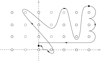
$(m_{1},n_{1})$                                                      $(m_{t},n_{t})$
                                                                                        $p_{3}$
                                        $(0,\delta)$                   $p_{4}$

Figure 3: The loop $\ell$ and numbers $a=4$, $b=3$ and $c=-2(1-9)=16$

We can now define a path $B_{t}$ of connections on $Y$.

Definition 5.3.

Set $B_{t}=-q(r)tidx$ for $0\leq t\leq\delta$, where $q(r)$ is defined in Equation (3.6).

Also set

$$B_{1}=\alpha^{a}\beta^{b}\gamma^{c}(-(n_{1}-[n_{1}])idy)=\gamma^{c}\alpha^{a}(-n_{1}idy).$$

Notice that $B_{1}|_{T}=a_{1}=-m_{1}idx-n_{1}idy.$

Finally, define $B_{t}$ for $\delta<t\leq 1$ to be any path of connections in normal form interpolating from $B_{\delta}$ to $B_{1}$ and satisfying $B_{t}|_{T}=a_{t}$. Such a path exists since the space of connections on $Y$ with a given normal form on the boundary is contractible.

Since the restrictions of $B_{t}$ and $C_{t}$ to the torus agree, and since they are in normal form, they can be glued together to form a path

$$A_{t}=B_{t}\cup_{a_{t}}C_{t}$$

of connections on $X$. This path satisfies all the requirements of Subsection 3.4, and hence we can apply Theorem 3.9. Notice that the flat connection $B_{1}$ depends only on the homotopy class (rel endpoints) of the path $(m_{t},n_{t}),\ t\in[\delta,1]$ in ${\mathbb{R}}^{2}-{\mathbb{Z}}^{2}$.

5.2 Computation of the spectral flow

Theorem 5.4.

Let $A_{t}$ be the path of connections on $X$ constructed above and let $a$ and $b$ be the integers defined above for the path $(m_{t},n_{t})$ (so $a=m_{1}$ and $b=[n_{1}]$). Then

$$SF(A_{t};X)=SF(A_{\eta};Z;P^{-})+2(a-b)-2.$$ (5.1)

ProofBy Theorem 3.9, we only need to show that $SF(A_{\bar{\sigma}\cdot\eta};Y;P^{+})=2(a-b)$. The path of connections $A_{\bar{\sigma}\cdot\eta}|_{Y}$ starts at the flat connection $-\delta idy$ and ends at $B_{1}$. Its projects under $Q$ to the path $\bar{\sigma}\cdot\eta$ in ${\mathbb{R}}^{2}-{\mathbb{Z}}^{2}$.

Recall that the path $\bar{\sigma}$ is the small quarter circle from $(0,\delta)$ to $(\delta,0)$ and that $\eta$ is just $(m_{t},n_{t})$ starting at $t=\delta$. Referring to the notation and results of Section 4, we see that the homotopy class rel boundary of the path $\bar{\sigma}\cdot\eta$ in ${\mathbb{R}}^{2}-{\mathbb{Z}}^{2}$ uniquely determines a word $w$ in $\alpha$ and $\beta$ in the group $G$. This word uniquely specifies a path $P$ in the Cayley graph, which we regard as a path of connections on the solid torus.

For example, the word $w=\alpha^{3}\beta\alpha^{-1}$ determines the path

$$P=E_{\alpha}\cdot\alpha E_{\alpha}\cdot\alpha^{2}E_{\alpha}\cdot\alpha^{3}E_{\beta}\cdot\alpha^{3}\beta\alpha^{-1}E_{\alpha}^{-1},$$

where $E_{\alpha}^{-1}$ means $E_{\alpha}$ traversed backwards. By construction, the endpoint of this path is $\alpha^{3}\beta\alpha^{-1}\cdot(-\tfrac{1}{2}idy)$.

Given any word $w$ in $\alpha$ and $\beta,$ the associated path $P$ goes from $-\frac{1}{2}idy$ to $w\cdot(-\frac{1}{2}idy)$. Thinking of $w$ as an element of $G$ and using Lemma 4.3 to put $w$ into normal form, it follows that

$$w=\alpha^{a}\beta^{b}\gamma^{c}$$

where $a=m_{1},b=[n_{1}]$ and $c$ is defined relative to the path $\bar{\sigma}\cdot\eta$ as in Definition 5.2. Thus, the terminal point of $P_{w}$ is the flat connection $\alpha^{a}\beta^{b}\gamma^{c}\cdot(-\frac{1}{2}idy).$

We now construct a path $\widetilde{P}$ by pre- and post-composing the given path $P$ so the initial and terminal points agree with those of the path $A_{\bar{\sigma}\cdot\eta}|_{Y}$. This is done by adding short segments of nontrivial, flat connections. This will not affect the spectral flow since any nontrivial representation $\rho\co\pi_{1}Y\to SU(2)$ has $H^{0+1}(Y;{\mathbb{C}}^{2}_{\rho})=0$.

Consider first the line segment from $(0,\delta)$ to $(0,\frac{1}{2})$ in ${\mathbb{R}}^{2}$. Since it misses the integer lattice, it lifts to a straight line from $-\delta idy$ to $-\frac{1}{2}idy$. This lift is a path of nontrivial flat connections on $Y$. Now consider the line segment from $(m_{1},[n_{1}]+\frac{1}{2})$ to $(m_{1},n_{1}).$ It also misses the integer lattice, hence it lifts to a straight line from $\alpha^{a}\beta^{b}\gamma^{c}\cdot(-\frac{1}{2}idy)$, the terminal point of $P$, to $\alpha^{a}\beta^{b}\gamma^{c}\cdot(-(n_{1}-[n_{1}])idy),$ the flat connection $B_{1}$. The second lift is also a path of nontrivial flat connections on $Y.$

Precomposing $P$ by the first lift and post-composing by the second defines a path $\widetilde{P}$ with the same ${\mathbb{C}}^{2}$-spectral flow as $P$. Notice that the initial and terminal points of $\widetilde{P}$ agree with those of $A_{\bar{\sigma}\cdot\eta}|_{Y}.$ By Theorem 4.9, if $g\in G$, then the spectral flow on $Y$ with $P^{+}$ boundary conditions along $g\cdot E_{\alpha}$ equals $2$ and along $g\cdot E_{\beta}$ equals $-2$. Thus the spectral flow along the path $P$ is equal to $2(a-b)$. But since the spectral flow along $\widetilde{P}$ is the same as that along $P$, and since $\widetilde{P}$ is homotopic rel endpoints to $A_{\bar{\sigma}\cdot\eta}|_{Y}$, this shows that $SF(A_{\bar{\sigma}\cdot\eta};Y;P^{+})=2(a-b)$ and completes the proof.

5.3 The Chern–Simons invariants

The Chern–Simons function is defined on the space ${\mathcal{A}}_{X}$ of connection 1–forms on a closed manifold $X$ by

$$cs(A)=\frac{1}{8\pi^{2}}\int_{X}{\rm tr}(A\wedge dA+\tfrac{2}{3}A\wedge A\wedge A).$$

With this choice of normalization, $cs\co{\mathcal{A}}_{X}\to{\mathbb{R}}$ satisfies $cs(g\cdot A)=cs(A)-\deg g$ for gauge transformations $g$ (recall that $g\cdot A=gAg^{-1}-dg~{}g^{-1}$). Since computing $cs$ modulo ${\mathbb{Z}}$ is not sufficient for the applications we have in mind, we work with connections rather than gauge orbits.

Using the same path $A_{t}=B_{t}\cup_{a_{t}}C_{t}$ of connections on $X=Y\cup_{T}Z$ as in Subsection 5.1, we show how to compute $cs(A_{1})\in{\mathbb{R}}$. This time, the initial data is a path of flat connections $C_{t}$ on $Z$ in normal form on the collar with $C_{0}$ trivial and $C_{1}$ extending flatly over $X$.

The restriction of $C_{t}$ to the boundary determines path $(m_{t},n_{t})$ (ie, $C_{t}|_{T}=-m_{t}idx-n_{t}idy$) which was used in Subsection 5.1 to construct a path $A_{t}$ of connections on $X$ starting at the trivial connection and ending at a flat connection $A_{1}$. Reparameterize the path $(m_{t},n_{t})$ so that the coordinates are differentiable. (It can always be made piecewise analytic by the results of [16], and hence using cutoff functions we can arrange that it is smooth.)

Theorem 5.5.

The Chern–Simons invariant of $A_{1}$ is given by the formula

$$cs(A_{1})=-c+2\int_{0}^{1}n{\frac{dm}{dt}}\ dt.$$

ProofWe follow the proof of Theorem 4.2 in [19], being careful not to lose integer information. Let $T(A)$ denote the transgressed second Chern form

$$T(A)={\frac{1}{8\pi^{2}}}{\rm tr}(dA\wedge A+{\frac{2}{3}}A\wedge A\wedge A).$$

Then

$$cs(A_{1})=\int_{Y}T(B_{1})+\int_{Z}T(C_{1})$$

since $A_{1}=B_{1}\cup C_{1}$ on $X=Y\cup_{T}Z$. We compute these terms separately, using the following lemma.

Lemma 5.6.

Let $W$ be an oriented 3–manifold with oriented boundary $T=S^{1}\times S^{1}$. Let $A_{t}$ be a path of flat connections in normal form on $W$. Assume that $A_{t}|_{T}=-m_{t}idx-n_{t}idy$, where $\{dx,dy\}$ is an oriented basis of $H_{1}(T;{\mathbb{Z}})$. Then

$$\int_{W}T(A_{1})-\int_{W}T(A_{0})=\int_{0}^{1}(m\tfrac{dn}{dt}-\tfrac{dm}{dt}n)dt.$$

ProofOrienting $I\times W$ and $I\times\partial W$ as products and using the outward normal first convention, one sees that the boundary

$$\partial(I\times W)=(\{1\}\times W)-(\{0\}\times W)-I\times\partial W.$$

The path of connections $A_{t}$ on $W$ can be viewed as a connection ${\bf A}$ on $I\times W$. Then the curvature form $F^{\bf A}$ equals $dt\wedge\omega$ for some $1$–form $\omega$. Hence $c_{2}({\bf A})=\tfrac{1}{4\pi^{2}}$tr$(F^{\bf A}\wedge F^{\bf A})=0$.

Using Stokes’ theorem as in [19], one computes that

$$0=\int_{I\times W}c_{2}({\bf A})=\int_{W}T(A_{1})-T(A_{0})-\int_{I\times\partial W}T({\bf a}),$$ (5.2)

where ${\bf a}$ denotes the connection $-m_{t}idx-n_{t}idy$ on $I\times\partial W$. Since $d{\bf a}=-\tfrac{dm}{dt}idtdx-\tfrac{dn}{dt}idtdy,$ it follows that

$$d{\bf a}\wedge{\bf a}=\left(-\tfrac{dm}{dt}n+m\tfrac{dn}{dt}\right)dxdy.$$

Clearly ${\bf a}\wedge{\bf a}\wedge{\bf a}=0$, so

$$T({\bf a})=\tfrac{1}{4\pi^{2}}(-\tfrac{dm}{dt}n+m\tfrac{dn}{dt})dtdxdy.$$

Hence

$$\int_{I\times\partial W}T({\bf a}) = {\tfrac{1}{4\pi^{2}}}\int_{I\times\partial W}(-\tfrac{dm}{dt}n+m\tfrac{dn}{dt})dtdxdy$$

$$= \int_{0}^{1}(-\tfrac{dm}{dt}n+m\tfrac{dn}{dt})dt.$$

Substituting this into Equation (5.2) finishes the proof of Lemma 5.6.

Returning to the proof of Theorem 5.5, we use Lemma 5.6 to compute $\int_{Z}T(C_{1})$. Since $C_{t}$ is a path of flat connections on $Z$ starting at the trivial connection, Lemma 5.6 implies that

$$\int_{Z}T(C_{1})=-\int_{0}^{1}(m\tfrac{dn}{dt}-\tfrac{dm}{dt}n)dt.$$

The sign change occurs because $\partial Z=-T$ as oriented manifolds.

Next we compute the term $\int_{Y}T(B_{1})$. Recall from Definition 5.3 that $B_{1}=\gamma^{c}\alpha^{a}(-n_{1}idy).$ Since $\gamma$ is a degree 1 gauge transformation supported in the interior of $Y$ and $cs(g\cdot A)=cs(A)-$deg$(g)$,

$$\int_{Y}T(B_{1})=-c+\int_{Y}T(\alpha^{a}(-n_{1}idy)).$$

Consider the path of flat connections on $Y$, $\widetilde{B}_{t}=\alpha^{a}(-tn_{1}idy),\ t\in[0,1]$. Then $\widetilde{B}_{0}=\alpha^{a}(\Theta)=-d(\alpha^{a})(\alpha^{a})^{-1}$ and $\widetilde{B}_{1}=\alpha^{a}(-n_{1}idy)$. The restriction of $\widetilde{B}_{t}$ to the torus is $\widetilde{B}_{t}|_{T}=\tilde{\alpha}^{a}(-tn_{1}idy)=-aidx-tn_{1}idy$. Recall that $a=m_{1}$. Applying Lemma 5.6 we conclude that

$$\int_{Y}T(\alpha^{a}(-n_{1}idy))=m_{1}n_{1}+\int_{Y}T(-d(\alpha^{a})(\alpha^{a})^{-1}).$$

But $\int_{Y}T(-d(\alpha^{a})(\alpha^{a})^{-1})=0$ since $-d(\alpha^{a})(\alpha^{a})^{-1}$ has no $dy$ component, thus

$$cs(A_{1})=-c+m_{1}n_{1}-\int_{0}^{1}(m{\tfrac{dn}{dt}}-{\tfrac{dm}{dt}}n)dt=-c+2\int_{0}^{1}\tfrac{dm}{dt}ndt.$$ ∎

5.4 Example: $\pm$ 1 Dehn surgery on the trefoil

In this section, we use our previous results to determine the ${\mathbb{C}}^{2}$–spectral flow and the Chern–Simons invariants for flat connections on the homology spheres obtained by $\pm 1$ surgery on the right–hand trefoil $K$. More general results for surgeries on torus knots will be given in Section 6.

The key to all these computations is a concrete description of the $SU(2)$ representation variety of the knot complement (see [26]). Let $K$ be the right hand trefoil knot in $S^{3}$ and let $Z$ be the 3–manifold with boundary obtained by removing an open tubular neighborhood of $K$. Its fundamental group has presentation

$$\pi_{1}Z=\langle x,y\mid x^{2}=y^{3}\rangle.$$

There are simple closed curves $\tilde{\mu}$ and $\tilde{\lambda}$ on $\partial Z=T$ intersecting transversely in one point called the meridian and longitude of the knot complement. We use the right hand rule to orient the pair $\tilde{\lambda},\tilde{\mu}$ (see Subsection 6.1 for more details). In $\pi_{1}Z$, $\tilde{\mu}$ represents $xy^{-1}$ and $\tilde{\lambda}$ represents $x^{2}(xy^{-1})^{-6}$ (cf. Equation (6.1)).

The representation variety ${\mathfrak{R}}_{SU(2)}(Z)$ can be described as the identification space of two closed intervals where the endpoints of the first interval are identified with two points in the interior of the second (see Figure 4). (In general, the representation variety of any torus knot complement is a singular 1–manifold with ‘T’ type intersections called $SU(2)$ bifurcation points, see [26].)

Figure 4: $SU(2)$ representations of the trefoil

Since $\tilde{\mu}$ normally generates $\pi_{1}Z,$ any abelian representation $\beta\co\pi_{1}Z\to SU(2)$ is uniquely determined by the image $\beta(\tilde{\mu})$. To each $t\in[0,\frac{1}{2}]$ we associate the abelian representation $\beta_{t}\co\pi_{1}Z\to SU(2)$ with $\beta_{t}(\tilde{\mu})=e^{2\pi it}$. Thus, the interval $[0,\frac{1}{2}]$ parameterizes the conjugacy classes of abelian or reducible representations.

The arc of nonabelian or irreducible conjugacy classes of representations can be parameterized by the open interval $(0,1)$ as follows. For $t\in[0,1]$, let $\rho_{t}\co\pi_{1}Z\to SU(2)$ be the representation with $\rho_{t}(x)=i$ and

$$\rho_{t}(y)=\cos(\tfrac{\pi}{3})+\sin(\tfrac{\pi}{3})(\cos(t\pi)i+\sin(t\pi)j).$$

In [26] it is proved that every irreducible $SU(2)$ representation of $\pi_{1}Z$ is conjugate to one and only one $\rho_{t}$ for some $t\in(0,1).$ The endpoints of $\rho_{t}$ coincide with the reducible representations at ${1/12}$ and ${5/12}$.

Restriction to the boundary defines a map ${\mathfrak{R}}_{SU(2)}(Z)\to{\mathfrak{R}}_{SU(2)}(T)$. To apply Theorems 5.4 and 5.5 to manifolds obtained by surgery on $K$, we need to lift the image ${\mathfrak{R}}^{*}_{SU(2)}(Z)\to{\mathfrak{R}}_{SU(2)}(T)$ under the branched cover $f\co{\mathbb{R}}^{2}\to{\mathfrak{R}}_{SU(2)}(T)$ of Equation (3.2). It is important to notice that $f$ depends on the surgery coefficients. Specifically, $f$ is defined in Equation (3.2) relative to the the meridian and longitude of the solid torus, as opposed to the meridian and longitude of the knot complement. We denote the former by $\mu$ and $\lambda$ and the latter by $\tilde{\mu}$ and $\tilde{\lambda}$. For the manifold $X_{k}$ obtained by $\frac{1}{k}$ surgery on $K$, we have $\mu=\tilde{\mu}\tilde{\lambda}^{k}$ and $\lambda=\tilde{\lambda}$.

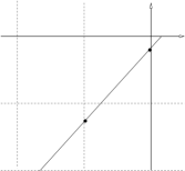
$A_{1}$
                                                        $A_{2}$

Figure 5: Two flat connections extending over $+1$ surgery on the right hand trefoil

For the Poincaré homology sphere (denoted here by $X_{+1}$), Proposition 6.8 implies that one such lift is given by the curve (see Figure 5)

$$R_{1}(t)=(1-t)(\tfrac{1}{12},0)+t(-\tfrac{19}{12},-2),\ \ 0\leq t\leq 1.$$

All other lifts are obtained by translating $R_{1}$ by integer pairs and/or reflecting it through the origin.

$$\begin{array}[]{|c| c c c|c|c|c|}\hline\cr&\ a&b&c&2\int m^{\prime}n&cs(A)&SF(\Theta,A)\\ \hline\cr A_{1}&0&-1&0&\frac{1}{120}&\frac{1}{120}&0\\ \hline\cr A_{2}&-1&-2&2&\frac{169}{120}&-\frac{71}{120}&0\\ \hline\cr\end{array}$$

Table 1: $X_{+1}=$ +1 surgery on the right hand trefoil

A representation $\rho\co\pi_{1}Z\to SU(2)$ extends over $X_{+1}$ if and only if $\rho(\mu)=1$, hence it follows that the irreducible representations of $X_{+1}$ correspond to the points of $R_{1}$ where the first coordinate is an integer. Figure 5 shows two such points which represent two flat connections $A_{1}$ and $A_{2}$. Let $(m_{t},n_{t})$ be the path described as the composition of the horizontal line segment from $(0,0)$ to $({\frac{1}{12}},0)$ with the path $R_{1}(s)$. Then $A_{1}$ and $A_{2}$ are the flat connections constructed as in Subsection 5.1 using the path $(m_{t},n_{t})$, stopping on the $R_{1}$ portion at $R_{1}(1/20)$ for $A_{1}$ and at $R_{1}(13/20)$ for $A_{2}$.

Using the path $A_{\xi\cdot\eta}$ constructed from $(m_{t},n_{t})$ as in Subsections 3.4 and 3.6, we compute the numbers $a_{i},b_{i},c_{i}$ associated to $A_{i}$ for $i=1,2.$ We get that $a_{1}=0,b_{1}=-1$, and $c_{1}=0$. Similarly $a_{2}=-1,b_{2}=-2$, and $c_{2}=2$.

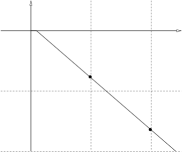
$A_{1}$
                                                                      $A_{2}$

Figure 6: Two flat connections extending over $-1$ surgery on the right hand trefoil

It follows from Theorem 6.5 below that $SF(A_{\eta}(t);Z;P^{-})=0$ for both $A_{1}$ and $A_{2}$. By Equation (5.1), $SF(\Theta,A_{i};X_{+1})=2(a_{i}-b_{i})-2$, we conclude that $SF(\theta,A_{i};X_{+1})=0$ for $i=1,2.$ One can also compute the integral term $2\int m^{\prime}n$ arising in Theorem 5.5, getting $2\int m^{\prime}n={\frac{1}{120}}$ for $A_{1}$ and $2\int m^{\prime}n={\frac{169}{120}}$ for $A_{2}$. These results are summarized Table 1.

Similar computations for the manifold $X_{-1}$ are given in Table 2. Here, Proposition 6.8 implies that the lift of the image of ${\mathfrak{R}}^{*}_{SU(2)}(Z)\to{\mathfrak{R}}_{SU(2)}(T)$ under $f\co{\mathbb{R}}^{2}\to{\mathfrak{R}}_{SU(2)}(T)$ is given by the curve

$$R_{1}(t)=(1-t)(\tfrac{1}{12},0)+t(\tfrac{29}{12},-2),\ \ 0\leq t\leq 1.$$

As before, the numbers $a,b$ and $c$ and the integral term $2\int m^{\prime}n$ can be easily computed from Figure 6.

Using these results, we will determine the rho invariants of flat connections on $X_{+1}$ and $X_{-1}$ in Subsection 5.5.

$$\begin{array}[]{|c| c c c|c|c|c|}\hline\cr&\ a&b&c&2\int m^{\prime}n&cs(A)&SF(\Theta,A)\\ \hline\cr A_{1}&1&-1&-2&-\frac{121}{168}&\frac{215}{168}&2\\ \hline\cr A_{2}&2&-2&-6&-\frac{529}{168}&\frac{479}{168}&6\\ \hline\cr\end{array}$$

Table 2: $X_{-1}=-1$ surgery on the right hand trefoil

5.5 The rho invariants

In this section, we present explicit formulas for the rho invariants based on our previous results. We first make clear which rho invariants we are computing. Following [3], an $SU(2)$ connection $A$ on $X$ determines the self-adjoint odd signature operator with ${\mathbb{C}}^{2}$ coefficients:

$$D_{A}\co\Omega^{0+2}_{X}\otimes{\mathbb{C}}^{2}\to\Omega^{0+2}_{X}\otimes{\mathbb{C}}^{2}.$$

The eta invariant of $D_{A}$, denoted here by $\eta_{A}(0)$, is the spectral invariant regularizing the signature; it is the analytic continuation to $s=0$ of

$$\eta_{A}(s)=\sum_{\lambda\neq 0}\frac{\hbox{sign}(\lambda)}{|\lambda|^{s}};$$

where the sum is over nonzero eigenvalues $\lambda$ of $D_{A}$.

If $A$ is a flat connection, then Atiyah, Patodi, and Singer show that the difference

$$\varrho_{X}(A)=\eta_{A}(0)-\eta_{\Theta}(0)$$

is a real number which is independent of the metric. Moreover, $\varrho_{X}(A)$ is gauge invariant and hence defines a function $\varrho_{X}\co{\mathfrak{M}}_{SU(2)}(X)\to{\mathbb{R}}$ on the flat $SU(2)$ moduli space of $X$. Using the holonomy map to identify flat connections $A$ and representations $\alpha\co\pi_{1}X\to SU(2)$, the rho invariant can therefore also be viewed as a real-valued function on ${\mathfrak{R}}_{SU(2)}(X)$.

The rho invariants considered in this paper are those associated to the canonical representation of $SU(2)$ on ${\mathbb{C}}^{2}$, not the adjoint representation on $su(2)$ which is more commonly studied in Donaldson and Floer theory. In the latter situation, Fintushel and Stern developed a technique for computing the (adjoint) rho invariants of $SU(2)$ representations of Seifert–fibered spaces by extending them over the mapping cylinder of the Seifert fibration, viewed as a 4–dimensional orbifold [17]. This method does not apply to our situation because generic fibers do not act trivially in the canonical representation as they do in the adjoint representation.

Theorem 5.7.

Suppose $C_{t}$ is a path of flat connections in normal form on $Z$ starting at the trivial connection and ending at a connection with trivial holonomy around $\mu$. Let $A_{1}$ be any flat connection $X=Y\cup_{T}Z$ which extends $C_{1}$. Then the rho invariant of $A_{1}$ is given by the formula

$$\varrho_{X}(A_{1}) = 2SF(A_{\eta}(t);Z;P^{-})+4(a-b+c)-2$$

$$-\dim(\ker D_{A_{1}})-8\int m^{\prime}n,$$

where $C_{t}|T=-m_{t}idx-n_{t}idy$, and $a,b,c$ are the integer homotopy invariants of the path $(m_{t},n_{t})$ defined in Subsection 5.1.

ProofThe rho invariant is gauge invariant so every flat connection on $X$ gauge equivalent to $A_{1}$ has the same rho invariant. Thus we are free to use the path $A_{t}$ of connections constructed in Subsection 5.1 from the path $C_{t}$ to compute $\varrho_{X}(A_{1}).$

A standard application of the Atiyah–Patodi–Singer index theorem shows that

$$SF(A_{t};X)=2cs(A_{1})+\tfrac{1}{2}\left(\varrho_{X}(A_{1})-\dim(\ker D_{\Theta})+\dim(\ker D_{A_{1}})\right).$$ (5.4)

This follows just as in the appendix to [24], keeping in mind that we are using the $(-\varepsilon,-\varepsilon)$-convention to compute spectral flow here whereas in that paper, the $(-\varepsilon,\varepsilon)$-convention is used (hence the sign change for the term $\dim(\ker D_{A_{1}})$).

Recall further that $\ker D_{\Theta}=H^{0+1}(X;{\mathbb{C}}^{2})\cong{\mathbb{C}}^{2}$. Using Theorem 5.5 and Corollary 5.4 to substitute into Equation (5.4) and solving for $\varrho_{X}(A_{1})$ yields Equation (5.7).

In general, from Equation (5.4), if $\dim(\ker D_{A})=0$, then

$$\varrho_{X}(A)=2SF(\Theta,A;X)-4cs(A)+2.$$ (5.5)

By Theorem 6.2, this holds for every nontrivial flat connection $A$ over a homology sphere $X$ obtained by surgery on a $(2,q)$ torus knot.

Example 5.8.

Suppose $K$ is the right hand trefoil and consider the two sets of connections on $X_{\pm 1}$, the homology spheres obtained by $\pm 1$ surgery on $K$. Then, referring to Tables 1 and 2 and utilizing Equation (5.5), we conclude that:

Case 1For $+1$ surgery on $K$, $\varrho_{X_{+1}}(A_{1})=59/30$ and $\varrho_{X_{+1}}(A_{2})=131/30.$

Case 2For $-1$ surgery on $K$, $\varrho_{X_{-1}}(A_{1})=37/42$ and $\varrho_{X_{-1}}(A_{2})=109/42.$

Notice that while the quantities in Tables 1 and 2 depend on the choice of gauge representatives $A_{1}$ and $A_{2}$, the rho invariants do not. We shall extend these computations considerably, first to all homology spheres obtained by Dehn surgery on the trefoil (Theorems 6.9 and 6.10) and later to all homology spheres obtained by surgery on a $(2,q)$ torus knot (Theorems 6.14 and 6.15).

5.6 The SU(3) Casson invariant

In [5], an invariant of homology 3–spheres $X$ was defined by counting, with sign, the number of irreducible $SU(3)$ representations of $\pi_{1}(X)$ and subtracting a correction term. The correction term is given by a sum of ${\mathbb{C}}^{2}$–spectral flows and Chern–Simons invariants applied to flat $SU(2)$ connections. One must typically incorporate the effect of perturbations on both of these sums, but in certain fortuitous cases the flat moduli space ${\mathfrak{M}}_{SU(3)}(X)$ is regular and no perturbations are needed. The aim of this subsection is to give a simple formula for the correction term in this special case.

To begin, we recall the definition of the $SU(3)$ Casson invariant (cf. Section 5 of [5]).

Definition 5.9.

The $SU(3)$ Casson invariant for a homology sphere $X$ is given by the sum

$$\lambda_{SU(3)}(X)=\lambda^{\prime}_{SU(3)}(X)+\lambda^{\prime\prime}_{SU(3)}(X)$$

where

$$\lambda^{\prime}_{SU(3)}(X) = \sum_{\quad[A]\in{{\mathfrak{M}}}^{*}_{SU(3),h}(X)}(-1)^{SF_{su(3)}(\Theta,A;X)}$$

$$\lambda^{\prime\prime}_{SU(3)}(X) = \sum_{[A]\in{{\mathfrak{M}}}^{*}_{SU(2),h}(X)}(-1)^{SF_{su(2)}(\Theta,A;X)}(SF(\theta,A;X)-2cs(\widehat{A})+1).$$

These are the first and second sums, respectively, of Definition 5.2 in [5]. All the spectral flows are taken with respect to the twisted odd signature operator $D_{A}$ (this was denoted $K_{A}$ in [5]). The notation $SF(\Theta,A;X)$ refers to the ${\mathbb{C}}^{2}$-spectral flow, ie, taking $SU(2)$ acting on ${\mathbb{C}}^{2}$ (and counting complex eigenvectors) just as above. (The analogous term $SF_{{\mathfrak{h}}^{\perp}}(\theta,A)$ in Definition 5.2 of [5] counts real eigenvectors, which adds a factor of $\frac{1}{2}$ in front of the second sum in Definition 5.2 of [5].). The notation $SF_{su(3)}$ and $SF_{su(2)}$ refers to the adjoint representations, ie, $SU(3)$ acting on $su(3)$ and $SU(2)$ acting on $su(2)$ by the adjoint representation (and count real eigenvectors). The function $h$ is a perturbation function used to perturb the flatness equations. Then ${\mathfrak{M}}^{*}_{SU(3),h}(X)$ denotes the moduli space of irreducible $h$-perturbed-flat $SU(3)$ connections on $X$, and similarly ${\mathfrak{M}}^{*}_{SU(2),h}(X)$ denotes the moduli space of irreducible $h$-perturbed-flat $SU(2)$ connections on $X$.

Notice that $\lambda_{SU(3)}$ is independent of the underlying orientation on the homology sphere. In fact this is true for $\lambda^{\prime}_{SU(3)}$ and $\lambda^{\prime\prime}_{SU(3)}$, namely $\lambda^{\prime}_{SU(3)}(-X)=\lambda^{\prime}_{SU(3)}(X)$ and $\lambda^{\prime\prime}_{SU(3)}(-X)=\lambda^{\prime\prime}_{SU(3)}(X)$.

Neither $\lambda^{\prime}_{SU(3)}(X)$ nor $\lambda^{\prime\prime}_{SU(3)}(X)$ is generally independent of the choice of perturbation $h$, which must be small and chosen so that ${\mathfrak{M}}_{SU(3),h}(X)$ is regular as in Definition 3.8 of [5]. To evaluate the correction term $\lambda^{\prime\prime}_{SU(3)}(X)$, one must also choose a representative $A$ for each $[A]\in{{\mathfrak{M}}}^{*}_{SU(2),h}(X)$ along with a nearby flat, reducible connection $\widehat{A}.$

In certain cases, including surgeries on $(2,q)$ torus knots, the $SU(3)$ moduli space is regular. In this case the invariant $\lambda_{SU(3)}$ is calculable without perturbing. In fact, whenever the $SU(2)$ moduli space is regular according to Definition 3.8 of [5], one can compute the correction term $\lambda^{\prime\prime}_{SU(3)}(X)$ in terms of $SU(2)$ rho invariants.

Theorem 5.10.

Suppose $X$ is a homology sphere with $H^{1}(X;su(2)_{A})=0$ and $H^{1}(X;{\mathbb{C}}^{2}_{A})=0$ for every irreducible flat $SU(2)$ connection $A$ on $X$. The first condition ensures that the moduli space ${\mathfrak{M}}_{SU(2)}^{*}(X)$ is a compact, 0–dimensional manifold, and the second implies that the points in ${\mathfrak{M}}_{SU(2)}^{*}(X)$ are not limits of arcs of irreducible flat $SU(3)$ connections. Then the correction term can be written as a sum of rho invariants, specifically

$$\lambda^{\prime\prime}_{SU(3)}(X)=\sum_{[A]\in{\mathfrak{M}}^{*}_{SU(2)}(X)}(-1)^{SF_{su(2)}(\Theta,A;X)}\varrho_{X}(A)/2.$$ (5.6)

ProofThis follows by taking $\widehat{A}=A$ in Definition 5.9 (which is allowed since ${\mathfrak{M}}^{*}_{SU(2)}(X)$ is regular as a subspace of ${\mathfrak{M}}_{SU(3)}(X)$ by hypothesis) and making a direct comparison with Equation (5.5).

In the next two examples, we present computations of the $SU(3)$ Casson invariant for $\pm 1$ surgery on the trefoil. In addition to the fact that the $SU(3)$ moduli space is regular, these cases avoid numerous other technical difficulties. For example, the sign of Equation (5.6) is constant for these manifolds. This goes back to a result of Fintushel and Stern which identifies the parity of the $su(2)$–spectral flow of irreducible flat $SU(2)$ connections on Brieskorn spheres (see [17] as well as the proof of Theorem 6.7). In the $SU(3)$ case, we know from [4] that the $su(3)$–spectral flow is even, which implies that $\lambda^{\prime}_{SU(3)}(X_{\pm 1})$ is given by simply counting the irreducible $SU(3)$ representations of $\pi_{1}(X_{\pm 1}).$ Moreover for $\pi_{1}(X_{\pm 1})$, all the important irreducible $SU(3)$ representations can be described in terms of representations of finite groups.

We compute the $SU(3)$ Casson invariant $\lambda_{SU(3)}$ for $\pm 1$ surgery on the right hand trefoil. Recall that (at least as unoriented manifolds) $X_{+1}\cong\Sigma(2,3,5)$ and $X_{-1}\cong\Sigma(2,3,7)$.

Example 5.11.

Consider first $X_{+1}.$ Case 1 of Example 5.8 shows that the moduli space of flat $SU(2)$ connections on $X_{+1}$ is

$${\mathfrak{M}}_{SU(2)}(X_{+1})=\{[\Theta],[A_{1}],[A_{2}]\},$$

where $\varrho_{X_{+1}}(A_{1})=59/30$ and $\varrho_{X_{+1}}(A_{2})=131/30.$

For any irreducible flat connection $A$ on $X_{+1}$, $SF_{su(2)}(\Theta,A;X_{+1})$ is odd (see Theorem 6.7). Thus Theorem 5.10 implies

$$\lambda^{\prime\prime}_{SU(3)}(X_{+1})=-\tfrac{1}{2}(\varrho_{X_{+1}}(A_{1})+\varrho_{X_{+1}}(A_{2}))=-19/6.$$

Since $\pi_{1}(X_{+1})$ is the binary icosahedral group (which is finite), it is well-known that it has two irreducible rank 3 representations. (Setting $\alpha_{i}=\operatorname{hol}_{A_{i}}$ for $i=1,2$, these are the two $SU(3)$ representations obtained by composing $\alpha_{i}\co\pi_{1}(X_{+1})\to SU(2)$ with the sequence of maps $SU(2)\to SO(3)\hookrightarrow SU(3)$ given by the standard projection followed by the natural inclusion.) Proposition 5.1 of [4] shows that the adjoint $su(3)$–spectral flow of $A_{1}$ and $A_{2}$ is even, hence $\lambda^{\prime}_{SU(3)}(X_{+1})=2$. Hence

$$\lambda_{SU(3)}(X_{+1})=\lambda^{\prime}_{SU(3)}(X_{+1})+\lambda^{\prime\prime}_{SU(3)}(X_{+1})=2-19/6=-7/6.$$

Example 5.12.

Now consider $X_{-1}.$ Case 2 of Example 5.8 shows that the moduli space of $SU(2)$ connections on $X_{-1}$ is

$${\mathfrak{M}}_{SU(2)}(X_{-1})=\{[\Theta],[A_{1}],[A_{2}]\},$$

where $\varrho_{X_{-1}}(A_{1})=37/42$ and $\varrho_{X_{-1}}(A_{2})=109/42.$ In this case, we know from Casson’s invariant that the $su(2)$–spectral flow has the opposite parity from the previous case, namely $SF_{su(2)}(\Theta,A_{i};M_{-1})$ is even for $i=1,2$. Theorem 5.10 implies

$$\lambda^{\prime\prime}_{SU(3)}(X_{-1})=\tfrac{1}{2}(\varrho_{X_{-1}}(A_{1})+\varrho_{X_{-1}}(A_{2}))=73/42.$$ (5.7)

In [4] it is shown that there are four irreducible $SU(3)$ representations of $\pi_{1}(X_{-1}).$ Two of these are obtained from the $SU(2)$ representations $\alpha_{i}=\operatorname{hol}_{A_{i}}$ as in the previous example and the other two are induced by representations of the quotient $PSL(2,{\mathbb{F}}_{7})$, which is a finite group of order $168$, as follows. Comparing the group presentations

$$\pi_{1}(X_{-1}) = \langle x,y,z,h\mid h\hbox{ central},x^{2}h=y^{3}h^{-1}=z^{7}h^{-1}=xyz=1\rangle$$

$$PSL(2,{\mathbb{F}}_{7}) = \langle x,y,z\mid x^{2}=y^{3}=z^{7}=xyz=[y,x]^{4}=1\rangle,$$

it is clear that $PSL(2,{\mathbb{F}}_{7})$ is the quotient of $\pi_{1}(X_{-1})$ by the normal subgroup $\langle h,[y,x]^{4}\rangle.$

It is well-known that $PSL(2,{\mathbb{F}}_{7})$ has precisely two irreducible $SU(3)$ representations (see page 96 of [11]), thus the two remaining $SU(3)$ representations of $\pi_{1}(X_{-1})$ are obtained from $PSL(2,{\mathbb{F}}_{7})$ by pullback. As before, Proposition 5.1 of [4] implies that the adjoint $su(3)$–spectral flow of each of the four irreducible $SU(3)$ representations is even. Hence $\lambda^{\prime}_{SU(3)}(X_{-1})=4$. Using this and Equation (5.7), it follows that

$$\lambda_{SU(3)}(X_{-1})=4+73/42=241/42.$$

Since the $SU(3)$ Casson invariant is unchanged by a change of orientation, we conclude that $\lambda_{SU(3)}(\Sigma(2,3,5))=-7/6$ and $\lambda_{SU(3)}(\Sigma(2,3,7))=241/42.$

6 Computations for torus knots

Given a 3–manifold $X$ and a flat $SU(2)$ connection $A$ on it, Theorems 5.4 and 5.5 determine the spectral flow and the Chern–Simons invariant of $A$ provided there exists a knot $K$ in $X$ so that $A$ is connected to the trivial connection $\Theta$ by a path of flat connections on the knot complement $Z=X-N(K)$. In this section we apply our methods to perform explicit computations for homology spheres obtained by surgery on a torus knot. Computing the spectral flow on the complement of a torus knot is not hard, and it is especially straightforward for $(2,q)$ torus knot complements (see Theorem 6.12). In this way, we reduce the computation of all the gauge theoretic invariants, including the rho invariants, to straightforward computations of the integers $a,b,c$, and the integral $2\int nm^{\prime}$.

Our aim is to compute the $SU(3)$ Casson invariant for surgeries on torus knots. In the general case, one needs to consider perturbed flat connections since the $SU(2)$ representation variety may not be cut out transversely as a subspace of the $SU(3)$ representation variety. For surgeries on $(2,q)$ torus knots, transversality holds so one can compute the $SU(3)$ Casson invariant without perturbing. As in Theorem 5.10, this has the happy consequence that the correction term $\lambda^{\prime\prime}_{SU(3)}$ can be expressed entirely in terms of the rho invariants. Using this approach, we compute $\lambda^{\prime\prime}_{SU(3)}$ for homology spheres obtained by surgery on a $(2,q)$ torus knot. Coupling these results with the computations of $\lambda^{\prime}_{SU(3)}$ in [4], we calculate $\lambda_{SU(3)}$ for surgeries on $K(2,q)$ for various $q$ and use this data to conclude that $\lambda_{SU(3)}$ is not a finite type invariant of order $6$.

6.1 Twisted cohomology of torus knot complements

We begin with a discussion of orientations and surgery conventions. Any knot $K$ in $S^{3}$ induces a decomposition of $S^{3}$ into two pieces, a tubular neighborhood $N(K)$ and the knot exterior $Z=S^{3}-N(K)$. This decomposition uniquely determines two isotopy classes of unoriented simple closed curves on the separating torus: $\tilde{\mu}$ is a curve which bounds a disc in $N(K)$ and $\tilde{\lambda}$ is a curve that bounds a surface in $Z$. These can be represented by smooth curves intersecting transversely in one point. Orient the pair $\{\tilde{\mu},\tilde{\lambda}\}$ so that $\tilde{\mu}\cdot\tilde{\lambda}=1$ with the outward normal first boundary orientation on $T=\partial(N(K))$.

For any integer $k$, consider the homology sphere $X=Y\cup_{T}Z$ obtained by performing $\tfrac{1}{k}$ surgery on $K$. This is the 3–manifold obtained by gluing the solid torus $Y=D^{2}\times S^{1}$ to $Z$ using a diffeomorphism of their boundaries which takes $\partial D^{2}\times\{1\}$ to $\tilde{\mu}\tilde{\lambda}^{k}$ and $\{1\}\times S^{1}$ to $\tilde{\lambda}.$ The curves

$$\mu=\tilde{\mu}\tilde{\lambda}^{k},\ \lambda=\tilde{\lambda}$$

are called the meridian and longitude of the Dehn filling $Y$. Notice that $\mu$ does not represent the usual meridian for the trefoil as a knot in $S^{3}$, but rather the meridian for the knot in $X$ which is the core of the Dehn filling.

Now consider, for $p$ and $q$ relatively prime and positive, the $(p,q)$ torus knot $K(p,q)$. This is the knot $K\co[0,2\pi]\to{\mathbb{R}}^{3}$ parameterized by $K(t)=((2+\cos qt)\cos pt,(2+\cos qt)\sin pt,-\sin qt).$ The restriction that $p$ and $q$ be positive is not serious; all the methods presented here are equally valid if either $p$ or $q$ is negative. Notice however that the result of $\frac{1}{k}$ surgery on $K(p,q)$ is diffeomorphic to that of $-\frac{1}{k}$ surgery on $K(p,-q)$ by an orientation-reversing diffeomorphism. Since the gauge theoretic invariants change in a predictable way under reversal of orientations, there is no loss in generality in assuming that $p$ and $q$ are positive.

The exterior $Z=S^{3}-N(K)$ of the $(p,q)$ torus knot $K$ has fundamental group

$$\pi_{1}Z=\langle x,y\mid x^{p}=y^{q}\rangle.$$

Choose $r,s\in{\mathbb{Z}}$ with the property that $pr+qs=1.$ Then the curves $\tilde{\mu}$ and $\tilde{\lambda}$ for $K(p,q)$ are represented in $\pi_{1}Z$ as

$$\tilde{\mu}=x^{s}y^{r}\quad\hbox{and}\quad\tilde{\lambda}=x^{p}(\tilde{\mu})^{-pq}.$$ (6.1)

For example, for the $(2,q)$ torus knot, one can take $s=1$ and $r=(1-q)/2$. Then $\tilde{\mu}=xy^{(1-q)/2}$ and $\tilde{\lambda}=x^{2}(\tilde{\mu})^{-2q}.$

Theorem 1 of [26] gives a general description of the variety of $SU(2)$ representations of torus knot groups. There it is shown that for a $(p,q)$ torus knot, ${\mathfrak{R}}_{SU(2)}(Z)$ is a connected, 1–dimensional singular manifold (smooth except for ‘T’ type intersections, called $SU(2)$ bifurcation points, discussed below.) Figures 4, 7, and 8 illustrate these representation varieties for several different torus knots.

Since $\tilde{\mu}$ normally generates $\pi_{1}Z,$ any reducible representation $\beta\co\pi_{1}Z\to SU(2)$ is uniquely determined by $\beta(\tilde{\mu})$. Throughout this section, we adopt the notation where $\beta_{s}$ for $s\in[0,\frac{1}{2}]$ refers to the reducible representation of $\pi_{1}Z$ which is uniquely determined up to conjugacy by the requirement that $\beta_{s}(\tilde{\mu})=e^{2\pi is}$. Since $\tilde{\lambda}$ lies in the commutator subgroup of $\pi_{1}Z$ (it bounds a Seifert surface) the reducible representation $\beta_{s}$ sends $\lambda$ to $1$ so $\beta_{s}(\tilde{\mu})=\beta_{s}(\mu)$.

The space ${\mathfrak{R}}^{*}_{SU(2)}(Z)$ of irreducible representations consists of $(p-1)(q-1)/2$ open arcs, the ends of which limit to distinct reducible representations. Thus, ${\mathfrak{R}}_{SU(2)}(Z)$ is the space obtained by identifying the endpoints of a collection of closed arcs with distinct interior points of the interval $[0,\tfrac{1}{2}]$. It follows that ${\mathfrak{R}}_{SU(2)}(Z)$ is path connected and any flat connection $A$ on a homology sphere obtained from surgery on a torus knot can be connected to the trivial connection $\Theta$ by a path of connections which are flat on $Z$ and which satisfy conditions 1–3 of Subsection 3.4.

The next result is crucial to computations of $SF(A_{\eta}(t);Z;P^{-})$ for torus knot complements. It identifies the kernel of $D_{A}$ with $P^{-}$ boundary conditions at any flat connection on $Z$.

Theorem 6.1.

Let $Z$ be the exterior of any $(p,q)$ torus knot and suppose $\alpha\co\pi_{1}(Z)\to SU(2)$ is a representation, defining a local coefficient system in ${\mathbb{C}}^{2}$.

1. If $\alpha$ is trivial, then $H^{0+1}(Z,\partial Z;{\mathbb{C}}^{2}_{\alpha})=0$.

2. If $\alpha$ is nontrivial, then $H^{0}(Z,\partial Z;{\mathbb{C}}^{2}_{\alpha})=H^{0}(Z;{\mathbb{C}}^{2}_{\alpha})=0$ and

   $$H^{1}(Z,\partial Z;{\mathbb{C}}^{2}_{\alpha})=H^{1}(Z;{\mathbb{C}}^{2}_{\alpha})=\begin{cases}{\mathbb{C}}^{2}&\text{if $\alpha(x^{p})=1$ and $\alpha(x)\neq 1\neq\alpha(y)$,}\\ 0&\hbox{otherwise.}\end{cases}$$

In particular if $A$ is a flat connection on $Z$ with nontrivial holonomy $\alpha=$hol_A then the kernel of $D_{A}$ with $P^{+}$ boundary conditions is isomorphic to ${\mathbb{C}}^{2}$ if $\alpha(x^{p})=1$, $\alpha(x)\neq 1$, and $\alpha(y)\neq 1$, and this kernel is zero otherwise.

ProofThe first statement is an easy exercise in cohomology since the coefficients are untwisted. The chain complex for the universal cover of $Z$ is computed by the Fox Calculus to be (with $\pi=\pi_{1}(Z)$)

$$0\to\ {\mathbb{Z}}[\pi]\ \smash{\mathop{\longrightarrow}\limits^{d_{2}}}\ {\mathbb{Z}}[\pi]\oplus{\mathbb{Z}}[\pi]\ \smash{\mathop{\longrightarrow}\limits^{d_{1}}}{\mathbb{Z}}[\pi]\ \to 0$$ (6.2)

with

$$d_{1}=\left[\begin{array}[]{c}x-1\\ y-1\end{array}\right]$$

and

$$d_{2}=\left[\begin{array}[]{cc}1+x+\cdots+x^{p-1}&\ x^{p}y^{-q}(1+y+y^{2}+\cdots+y^{q-1})\end{array}\right].$$

The cohomology $H^{*}(Z;{\mathbb{C}}^{2}_{\alpha})$ is defined to be the homology of the chain complex obtained by applying Hom${}_{{\mathbb{Z}}[\pi]}(-,{\mathbb{C}}^{2})$ to the complex (6.2), where $\pi$ acts on ${\mathbb{C}}^{2}$ via $\alpha$. The differentials are obtained by replacing $x$ and $y$ in the matrices $d_{2}$ and $d_{1}$ by $\alpha(x)$ and $\alpha(y)$ and taking the transpose. Denote by $d_{1}(\alpha)$ and $d_{0}(\alpha)$ the resulting differentials.

Clearly $d_{0}(\alpha)=0$ if and only if $\alpha$ is trivial. Thus if $\alpha$ is nontrivial, then $H^{0}(Z;{\mathbb{C}}^{2}_{\alpha})=0$. On the other hand, if $\alpha$ is nontrivial and $\alpha(x)=1$ then $\alpha(y)$ must be a nontrivial $q$–th root of unity and it follows that $d_{1}(\alpha)=\left[\begin{matrix}p\\ q\end{matrix}\right]$ and $d_{0}(\alpha)=[0\quad{\alpha(y)-1}]$. Since $\alpha(y)\neq 1,$ we see that $\ker d_{1}(\alpha)=\operatorname{im}d_{0}(\alpha)$. This implies $H^{1}(Z;{\mathbb{C}}^{2}_{\alpha})=0$.

Similar arguments apply and give the same conclusion if $\alpha$ is nontrivial and $\alpha(y)=1.$

So assume $\alpha(x)\neq 1$ and $\alpha(y)\neq 1.$ This implies that $\operatorname{im}d_{1}(\alpha)$ has complex dimension 2. If $\alpha(x^{p})=1$, then $\alpha(x)$ is a nontrivial $p$–th root of unity, which implies $1+\alpha(x)+\cdots+\alpha(x^{p-1})=0.$ Since $x^{p}=y^{q},$ it follows also that $\alpha(y)$ is a nontrivial $q$–th root of unity. Thus $d_{2}(\alpha)$ is the zero map and so $H^{1}(Z;{\mathbb{C}}^{2}_{\alpha})=\ker d_{1}(\alpha)/\operatorname{im}d_{0}(\alpha)$ is isomorphic to ${\mathbb{C}}^{2}$ in this case.

On the other hand, if $\alpha(x^{p})\neq 1,$ then $\alpha(x)$ is not a $p$–th root of unity. Hence $d_{1}(\alpha)$ is not the zero map and this forces $H^{1}(Z;{\mathbb{C}}^{2}_{\alpha})=0.$

We have seen (Equation (3.4)) that if $\alpha$ restricts nontrivially to $T=\partial Z$, then the cohomology of $T$ vanishes. Of course, since the meridian normally generates $\pi_{1}Z,$ any nontrivial representation $\alpha$ of $\pi_{1}Z$ pulls back to a nontrivial representation of $\pi_{1}T$. Now the long exact sequence in cohomology shows that $H^{i}(Z;{\mathbb{C}}^{2}_{\alpha})=H^{i}(Z,\partial Z;{\mathbb{C}}^{2}_{\alpha})$. The last statement follows from Proposition 2.10.

The characterization of the representation varieties ${\mathfrak{R}}_{SU(2)}(Z)$ of torus knot groups in [26] shows that $\operatorname{hol}_{A_{t}}(x)$ is constant (up to conjugacy) along paths of irreducible representations. Let $A$ be a flat connection on $Z$ with nontrivial holonomy and set $\alpha=\operatorname{hol}_{A}$. Use Proposition 2.10 to identify $H^{1}(Z;{\mathbb{C}}^{2}_{\alpha})$ with the kernel of $D_{A}$ on $Z$ with $P^{-}$ boundary conditions. Then Theorem 6.1 implies the following result.

Theorem 6.2.

If $A_{t}$ is a path of irreducible flat $SU(2)$ connections on the complement $Z$ of a $(p,q)$ torus knot, then the dimension of $H^{1}(Z;{\mathbb{C}}^{2}_{A_{t}})$ is independent of $t$. In particular $SF(A_{t};Z;P^{-})=0.$ Moreover, if $p=2$ then $\dim H^{1}(Z;{\mathbb{C}}^{2}_{A_{t}})=0$ for all $t$.

6.2 Jumping points and SU(2) bifurcation points

As we have already seen, the representation variety ${\mathfrak{R}}_{SU(2)}(Z)$ of the complement of a torus knot can be described as the space obtained by identifying endpoints of $(p-1)(q-1)/2$ closed arcs with interior points in the line segment $[0,\frac{1}{2}]$ parameterizing the reducibles. The non-smooth points, which are precisely where the arcs are attached, are called $SU(2)$ bifurcation points. It is a simple matter to characterize the $SU(2)$ bifurcation points (for torus knots) in terms of the Alexander polynomial, although which pairs of bifurcation points are endpoints of the same arc of irreducibles is a more subtle problem. However, if $p=2,$ the answer is simple because the arcs are glued in a nested way (see Proposition 6.5).

Closely related to the $SU(2)$ bifurcation points are the ${\mathbb{C}}^{2}$ jumping points. These play a central role in determining $SF(A_{\eta};Z;P^{-}),$ the spectral flow along the knot complement.

Definition 6.3.

Suppose $Z$ is the complement of a knot $K$ in a homology sphere $X$.

1. The ${\mathbb{C}}^{2}$ jumping points are the gauge orbits of nontrivial reducible flat $SU(2)$ connections $A$ on $Z$ where the kernel of $D_{A}$ with $P^{-}$ boundary conditions jumps up in dimension. This is the set of reducible flat connections $A$ so that $H^{1}(Z;{\mathbb{C}}^{2}_{A})\neq 0$.

2. The $SU(2)$ bifurcation points are gauge orbits of reducible flat connections $A$ on $Z$ which are limits of irreducible, flat connections.

Theorem 6.2 implies that for torus knot complements, only certain reducible flat connections are ${\mathbb{C}}^{2}$ jumping points. They are characterized in terms of the roots of the Alexander polynomial by the following theorem, which is reminiscent of the characterization of the $SU(2)$ bifurcation points in terms of square roots of the Alexander polynomial [26].

Theorem 6.4.

Suppose $K$ is the $(p,q)$ torus knot and $Z$ is its exterior. Given a reducible, flat, nontrivial $SU(2)$ connection $A$, the kernel of $D_{A}$ with $P^{-}$ boundary conditions is nontrivial if and only if $\operatorname{hol}_{A}(\tilde{\mu})$ is a root of the Alexander polynomial

$$\Delta_{K}(t)=\frac{(t^{pq}-1)(t-1)}{(t^{p}-1)(t^{q}-1)}.$$

ProofLet $\alpha=\operatorname{hol}_{A}$ be the reducible representation of $\pi_{1}Z$ associated with $A.$ By Theorem 6.1, $H^{1}(Z,\partial Z;{\mathbb{C}}^{2}_{\alpha})\neq 0$ if and only if $\alpha(x)$ has order $p^{\prime}$ and $\alpha(y)$ has order $q^{\prime}$ for $p^{\prime}\neq 1\neq q^{\prime}$, where $p^{\prime}$ divides $p$ and $q^{\prime}$ divides $q$. Since $p^{\prime}$ and $q^{\prime}$ are relatively prime, this implies that $\alpha(x)$ and $\alpha(y)$ generate a cyclic group of order $p^{\prime}q^{\prime}$ equal to $\langle\alpha(\tilde{\mu})\rangle$. Thus $\operatorname{hol}_{A}(\tilde{\mu})\neq 1$ is a $pq$–th root of unity, but it is neither a $p$–th root nor a $q$–th root of unity.

For torus knots, the roots of $\Delta_{K}(t)$ all lie on the unit circle. Thus ${\mathbb{C}}^{2}$ jumping points correspond to the reducible representations $\beta_{t}$ where $e^{2\pi is}$ is a root of $\Delta_{K}$. Since we always use $[0,\frac{1}{2}]$ to parameterize reducible $SU(2)$ representations, we will simply say $s\in[0,\frac{1}{2}]$ is a ${\mathbb{C}}^{2}$ jumping point if $\beta_{s}$ is. Similarly, we say that $s$ is an $SU(2)$ bifurcation point if $\beta_{s}$ is.

We give two quick examples. First, if $K$ is the trefoil then $\Delta_{K}(t)=t^{2}-t+1$. Its roots are $e^{\pm\pi i/3}$. This gives one ${\mathbb{C}}^{2}$ jumping point at $s={1/6}$ (this is the black dot in Figure 4). By [26], the $SU(2)$ bifurcation points are the solutions to $\Delta_{K}(t^{2})=0$. So for the trefoil, ${1/12}$ and ${5/12}$ are the $SU(2)$ bifurcation points. (These are just the square roots of the ${\mathbb{C}}^{2}$ jumping point.) Next, if $K$ is the $(2,5)$ torus knot, then $\Delta_{K}(t)=t^{4}-t^{3}+t^{2}-t+1$. Its roots are $e^{\pm\pi i/5}$ and $e^{\pm 3\pi i/5}$, yielding two ${\mathbb{C}}^{2}$ jumping points at ${1/10}$ and ${3/10}$. There are four $SU(2)$ bifurcation points: $\{\frac{1}{20},\frac{3}{20},\frac{7}{20},\frac{9}{20}\}$. Generalizing to $(2,q)$ torus knots, we obtain the following proposition.

Proposition 6.5.

Suppose $Z$ is the exterior of a $(2,q)$ torus knot and consider its $SU(2)$ representation variety ${\mathfrak{R}}_{SU(2)}(Z).$ Parameterize the reducible representations by $[0,\frac{1}{2}]$ as above. Then there are $(q-1)/2$ arcs of irreducible representations, indexed as $\widehat{R}_{\ell}$ for $\ell=1,\ldots,(q-1)/2$, such that $\widehat{R}_{\ell}$ is attached to $[0,\frac{1}{2}]$ at the $SU(2)$ bifurcation points $\frac{2\ell-1}{4q}$ and $\frac{1}{2}-\frac{2\ell-1}{4q}.$ Thus the arcs of irreducible representations are nested.

Notice further that the set of $SU(2)$ bifurcation points

$$\{\tfrac{2\ell-1}{4q},\tfrac{1}{2}-\tfrac{2\ell-1}{4q}\mid\ell=1,\ldots,(q-1)/2\}$$

is disjoint from the set

$$\{\tfrac{2\ell-1}{2q}\mid\ell=1,\ldots,(q-1)/2\}$$

of ${\mathbb{C}}^{2}$ jumping points.

ProofThe Alexander polynomial of $K(2,q)$ is $\Delta_{K}(t)=\frac{t^{q}+1}{t+1}$ and its roots are the $q$–th roots of $-1$ different from $-1.$ Theorem 6.4 easily identifies the ${\mathbb{C}}^{2}$ jumping points as the set $\{\tfrac{2\ell-1}{2q}\mid\ell=1,\ldots,(q-1)/2\}$. The $SU(2)$ bifurcation points correspond to the reducible representations $\beta$ with $\beta(\tilde{\mu}^{2})$ a root of $\Delta_{K}(t)$ [26]. Taking square roots gives the set $\{\tfrac{2\ell-1}{4q},\frac{1}{2}-\frac{2\ell-1}{4q}\mid\ell=1,\ldots,(q-1)/2\}$ of $SU(2)$ bifurcation points.

The arcs $\widehat{R}_{\ell}$ can be described as follows. Since $\pi_{1}Z=\langle x,y\mid x^{2}=y^{q}\rangle$ has infinite cyclic center generated by $x^{2},$ if $\alpha$ is irreducible then $\alpha(x^{2})=-1$ (the centralizer of any nonabelian subgroup of $SU(2)$ is $\pm 1$). Conjugating if necessary, we have $\alpha(x)=i$. Similarly, $\alpha(y)$ can be conjugated to lie in the $ij$–plane and must be a $q$–th root of $-1.$ Drawing the great circles from $1$ to $\alpha(x)$ and from $1$ to $\alpha(y)$, one can use the angle between the great circles to parameterize the arcs $\widehat{R}_{\ell}$ as in the proof of Theorem 1 in [26].

We will be even more specific. For $\ell=1,\ldots,(q-1)/2$ define a 1–parameter family of representations $\alpha_{\ell,t}\co\pi_{1}Z\to SU(2)$ for $t\in[0,1]$ by setting $\alpha_{\ell,t}(x)=i$ and

$$\alpha_{\ell,t}(y)=\cos(\tfrac{(2\ell-1)\pi}{q})+\sin(\tfrac{(2\ell-1)\pi}{q})(i\cos(\pi t)+j\sin(\pi t)).$$

These representations are irreducible except at the endpoints. The meridian of $K(2,q)$ is represented in $\pi_{1}Z$ by $\tilde{\mu}=xy^{(1-q)/2}$, and a simple computation shows that the endpoints of $\alpha_{\ell}$ are the reducible representations $\beta_{s}$ for $s\in\left\{\frac{q-2\ell-2}{4q},\frac{1}{2}-\frac{q-2\ell-2}{4q}\right\}$. As $\ell$ ranges from $1$ to $(q-1)/2$, the associated pairs of points in $[0,\frac{1}{2}]$ are nested ($\alpha_{\ell,t}$ parameterizes the arc $\widehat{R}_{(q-1)/2-\ell}$.)

$K(2,5)$                     $K(2,7)$                              $K(2,9)$

Figure 7: $SU(2)$ representation varieties of $(2,q)$ torus knot groups

Figures 7 and 8 show the $SU(2)$ representation varieties for several torus knots. The horizontal line segment denotes the reducibles, and the ${\mathbb{C}}^{2}$ jumping points are dots. The curved arcs are the irreducible components $\widehat{R}_{\ell}$.

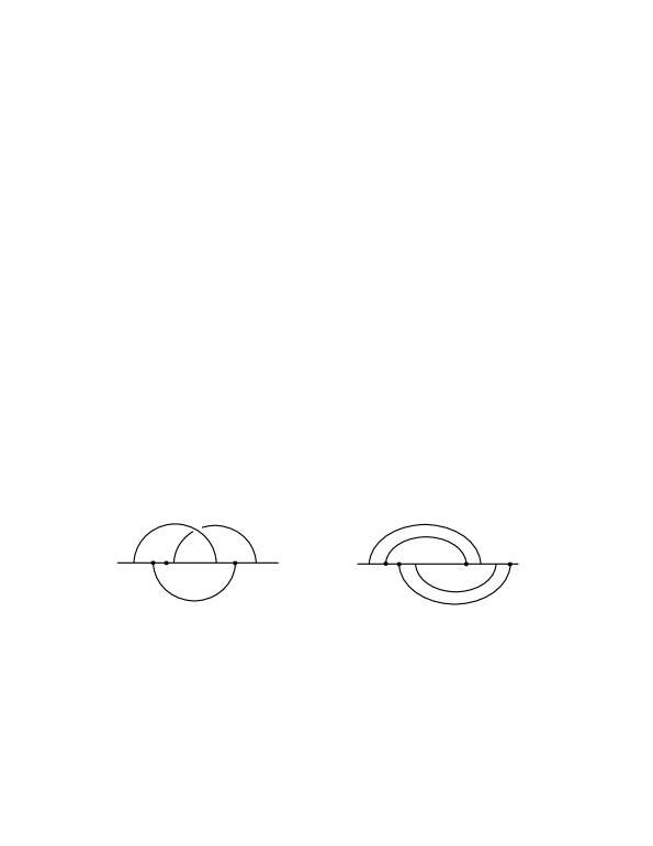
$K(3,4)$                                       $K(3,5)$

Figure 8: $SU(2)$ representation varieties of $(p,q)$ torus knot groups

Comparing Figures 7 and 8, one sees that most of the assertions of Proposition 6.5 fail for arbitrary $(p,q)$ torus knots. The sets of $SU(2)$ bifurcation points and ${\mathbb{C}}^{2}$ jumping points are not in general disjoint. Nor are the irreducible components nested as for $K(2,q)$. For $K(p,q)$, one can still use Theorem 6.4 to characterize the ${\mathbb{C}}^{2}$ jumping points, they occur at the reducible representations $\beta_{s}$ where $\beta_{s}(\tilde{\mu})=e^{2\pi is}$ is a $pq$–th root of unity which is neither a $p$–th root nor a $q$–th root of unity.

Corollary 6.6.

Suppose $X$ is a homology sphere obtained by surgery on a $(2,q)$ torus knot and $A$ is a nontrivial flat $SU(2)$ connection on $X.$ Then $H^{i}(X;{\mathbb{C}}^{2}_{A})=0=H^{i}(X;su(2)_{A})$ for all $i$. Hence, ${\mathfrak{M}}^{*}_{SU(2)}(X)$ is regular as a subset of ${\mathfrak{M}}_{SU(3)}(X)$ and the correction term $\lambda^{\prime\prime}_{SU(3)}(X)$ can be computed in terms of $SU(2)$ rho invariants.

ProofSince $X$ is a homology sphere, any nontrivial flat $SU(2)$ connection is irreducible. The restriction of such a connection to $Z$ is irreducible (since $\pi_{1}(Y)\cong{\mathbb{Z}}$), and its restriction to $T$ is nontrivial since the meridian $\tilde{\mu}$ normally generates $\pi_{1}Z$. Theorem 6.2 implies that $H^{1}(Z;{\mathbb{C}}^{2}_{A})=0$, and the corollary follows from the computations of Subsection 3.2 using the Mayer–Vietoris sequence. (The vanishing of first cohomology with both $su(2)$ and ${\mathbb{C}}^{2}$ coefficients is the definition of regularity in [5].) The corollary reflects a rather special property of $(2,q)$ torus knots. If $p,q>2$ and $X$ is a homology sphere obtained by surgery on $K(p,q)$ then there exists an irreducible $SU(2)$ representation which is the limit of an arc of irreducible $SU(3)$ representations, and hence ${\mathfrak{M}}^{*}_{SU(2)}(X)$ is not regular (when viewed as a subset of ${\mathfrak{M}}_{SU(3)}(X)$), although it is a compact 0–dimensional manifold.

Results of Fintushel and Stern shows that, for homology spheres $X$ obtained by surgery on a torus knot, ${\mathfrak{R}}^{*}_{SU(2)}(X)$ is a finite set of points and the parity of $SF_{su(2)}(\Theta,A;X)$ is independent of $[A]\in{\mathfrak{M}}^{*}_{SU(2)}(X)$. Corollary 6.6 and Theorem 5.10 then imply that, for surgeries on a $(2,q)$ torus knot,

$$\lambda^{\prime\prime}_{SU(3)}(X)=\pm{\tfrac{1}{2}}\sum_{[A]\in{\mathfrak{M}}^{*}_{SU(2)}(X)}\varrho_{X}(A).$$

The next result determines the sign. Recall if $\Delta_{K}(t)$ denotes the symmetrized Alexander polynomial of the knot $K$, then $\Delta_{K}^{\prime\prime}(1)$ equals twice Casson’s invariant of the knot ([1]). For the torus knot $K=K(2,q)$, $\Delta^{\prime\prime}_{K}(1)=(1-q^{2})/4$.

Theorem 6.7.

Let $K$ be the $(2,q)$ torus knot. Assume $k>0$ and denote by $X_{\pm k}$ the result of $\pm\frac{1}{k}$ surgery on $K.$ By Corollary 6.6, the ${\mathfrak{M}}_{SU(2)}(X_{\pm k})$ is regular as a subspace of ${\mathfrak{M}}_{SU(3)}(X_{\pm k})$. If $b=(q^{2}-1)/4$ then the moduli spaces ${\mathfrak{M}}_{SU(2)}^{*}(X_{k})$ and ${\mathfrak{M}}_{SU(2)}^{*}(X_{-k})$ consist of $kb$ points.

1. Writing ${\mathfrak{M}}_{SU(2)}(X_{k})=\{[\Theta],[A_{1}],\ldots,[A_{kb}]\}$, then $SF_{su(2)}(\Theta,A_{i};X_{k})$ is odd and

   $$\lambda^{\prime\prime}_{SU(3)}(X_{k})=-{\tfrac{1}{2}}\sum_{i=1}^{kb}\varrho_{X_{k}}(A_{i}).$$ (6.3)

2. Writing ${\mathfrak{M}}_{SU(2)}(X_{-k})=\{[\Theta],[A_{1}],\ldots,[A_{kb}]\}$, then $SF_{su(2)}(\Theta,A_{i};X_{-k})$ is even and

   $$\lambda^{\prime\prime}_{SU(3)}(X_{-k})={\tfrac{1}{2}}\sum_{i=1}^{kb}\varrho_{X_{-k}}(A_{i}).$$ (6.4)

ProofSuppose $X$ is a homology sphere obtained by a positive surgery on $K(p,q).$ We claim that if $A$ is an irreducible flat $SU(2)$ connection on $X$, then $SF_{su(2)}(\Theta,A;X)$ is odd. Theorem 5.10 then implies the first assertion.

By Taubes’ theorem [31] and the surgery formula for Casson’s invariant, this implies that $SF_{su(2)}(\Theta,A;X)$ is even in case $X$ is obtained by a negative surgery on $K(p,q)$, so the second assertion follows from the first.

Since Casson’s knot invariant is positive for all $(2,q)$ torus knots, it suffices to check one example, which we take to be the Poincaré homology sphere.

First, consider a path $A_{t}$ of $SU(2)$ connections on a homology sphere $X$ with $A_{i}$ flat for $i=0,1$. Let $\alpha_{i}=\operatorname{hol}_{A_{i}}$ for $i=0,1$ be the associated $SU(2)$ representations. Applying the Atiyah–Patodi–Singer index theorem as in the proof of Theorem 5.7 (cf. Equation (5.4)), we see that

$$SF_{su(2)}(A_{t};X) = 8(cs(A_{1})-cs(A_{0}))+\frac{1}{2}\left(\varrho_{X}({\rm ad}\,\alpha_{1})-\varrho_{X}({\rm ad}\,\alpha_{0})\right)$$ (6.5)

$$\hskip-50.58878pt+\ \frac{1}{2}\left(\dim H^{0+1}(X;su(2)_{\alpha_{1}})-\dim H^{0+1}(X;su(2)_{\alpha_{0}})\right),$$

where the rho invariants are defined relative to the odd signature operator acting on $su(2)$–forms via the adjoint action. (Comparing this to the formula at the end of Section 7 in [24], the sign discrepancies are explained by the fact that in this paper, we are using the $(-\varepsilon,-\varepsilon)$ convention for spectral flow.)

Now consider the Poincaré homology sphere $X$, defined here to be $+1$ surgery on the right hand trefoil. Consider a path from $\Theta$ to the flat connection $A_{1}$ constructed in Section 5.4. Since $\pi_{1}X$ is finite, one can compute that $\varrho_{X}({\rm ad}\,\alpha_{1})=\pm\frac{73}{15}$ by standard methods [17, 2]. The sign ambiguity comes about because the answer depends on how $X$ is oriented. This problem can be resolved since we know that $cs(A_{1})=\frac{1}{120}$ by the computations in Subsection 5.4. Applying Equation (6.5) to the path $A_{t}$, we see that the only way the left hand side can be an integer is if $\varrho_{X}({\rm ad}\,\alpha_{1})=\frac{73}{15}$, in which case $SF_{su(2)}(\Theta,A_{1};X)=1$, which is odd, as claimed.

RemarkIt is well-known that, at least as unoriented manifolds, $\tfrac{1}{k}$-surgery on a torus knot yields a Brieskorn homology sphere. These spaces admit a natural orientation as the link of an algebraic singularity. Using standard handlebody methods (or alternatively, using the fact that the $su(2)$–spectral flow from the trivial connection to a flat $SU(2)$ connection on a Brieskorn sphere is even [17]) it follows that, as oriented manifolds,

$$X_{k}\cong-\Sigma(2,q,2qk-1)\quad\text{ and }\quad X_{-k}\cong\Sigma(2,q,2qk+1).$$

Theorems 6.7 and 5.7 give a method for computing $\lambda^{\prime\prime}_{SU(3)}$ for surgeries on $(2,q)$ torus knots. Combining this with the computations of $\lambda^{\prime}_{SU(3)}$ given in [4], we shall determine $\lambda_{SU(3)}$ for homology spheres obtained by surgery on $K(2,q)$. The analogous computation for $K(p,q)$ is complicated by the fact that one must first apply a perturbation to make the moduli space regular, so we postpone the calculations for surgeries on other torus knots to a future article.

Consider the complement $Z$ of $K(p,q)$, with $\partial Z=T$, the torus. Recall that ${\mathfrak{R}}_{SU(2)}(T)$ denotes the variety of conjugacy classes of $SU(2)$ representations of $\pi_{1}T$. Any choice of generators $x,y\in\pi_{1}T={\mathbb{Z}}\oplus{\mathbb{Z}}$ determine a branched cover ${\mathbb{R}}^{2}\to{\mathfrak{R}}_{SU(2)}(T)$ by assigning to the pair $(m,n)\in{\mathbb{R}}^{2}$ the conjugacy class of the homomorphism taking $x$ to $e^{2\pi im}$ and $y$ to $e^{2\pi in}$. (See Equation (3.2).) We will need to consider the cases $x=\tilde{\mu}\tilde{\lambda}^{k}$ and $y=\tilde{\lambda}$ for various $k$ simultaneously. Thus we introduce the notation

$$f_{k}\co{\mathbb{R}}^{2}\to{\mathfrak{R}}_{SU(2)}(T)$$

for the map taking $(m,n)$ to the conjugacy class of the homomorphism $\alpha\colon$$\pi_{1}T\to SU(2)$ satisfying $\alpha(\tilde{\mu}\tilde{\lambda}^{k})=e^{2\pi im}$ and $\alpha(\tilde{\lambda})=e^{2\pi in}$. Letting $g_{k}\co{\mathbb{R}}^{2}\to{\mathbb{R}}^{2}$ denote the linear map

$$g_{k}(m,n)=(m+kn,n)$$ (6.6)

we see that

$$f_{0}=f_{k}\circ g_{k}.$$

Now consider the restriction map ${\mathfrak{R}}^{*}_{SU(2)}(Z)\to{\mathfrak{R}}_{SU(2)}(T)$. Each component of ${\mathfrak{R}}^{*}_{SU(2)}(Z)$ is an open arc. Proposition 6.5 enumerates these in the special case of $K(2,q)$; the path components are denoted $\widehat{R}_{\ell}$. The image in ${\mathfrak{R}}_{SU(2)}(T)$ of each arc misses the branch points since the branch points correspond to central representations of $\pi_{1}T$, but $\tilde{\mu}$ cannot be sent to the center $\pm 1$ by an irreducible (ie, nonabelian) representation since it is a normal generator of $\pi_{1}Z$. Thus each path component of ${\mathfrak{R}}^{*}_{SU(2)}(Z)$ lifts to ${\mathbb{R}}^{2}$.

We claim that any such lift using the cover $f_{0}\co{\mathbb{R}}^{2}\to{\mathfrak{R}}_{SU(2)}(T)$ takes the components of ${\mathfrak{R}}^{*}_{SU(2)}(Z)$ to arcs of slope $-pq$. One can see this as follows. If $\alpha_{t}\co\pi_{1}Z\to SU(2)$ is any continuous path of irreducible representations, then it can be conjugated so that $\alpha_{t}(\tilde{\mu})$ and $\alpha_{t}(\tilde{\lambda})$ lie in the standard $U(1)$ subgroup of $SU(2)$. If $\alpha_{t}$ is irreducible, then $\alpha_{t}(x^{p})=\pm 1$. Writing $\alpha_{t}(\tilde{\mu})=e^{2\pi im_{t}}$ and $\alpha_{t}(\tilde{\lambda})=e^{2\pi in_{t}}$, then Equation (6.1), namely that $\tilde{\lambda}=x^{p}(\tilde{\mu})^{-pq}$, shows that $pq\,m_{t}+n_{t}$ is constant.

To understand how the arcs in ${\mathfrak{R}}^{*}_{SU(2)}(Z)$ lift using the cover $f_{k}\co{\mathbb{R}}^{2}\to{\mathfrak{R}}_{SU(2)}(T)$, that is, with respect to $\mu$ and $\lambda$ for the homology sphere obtained by $\tfrac{1}{k}$ surgery on $K(p,q)$, one just applies the map $g_{k}$ of Equation (6.6). Thus each arc lifts using $f_{k}$ to arcs in ${\mathbb{R}}^{2}$ of slope $\tfrac{pq}{kpq-1}$.

The following proposition completes the identification of the lifts of each arc $\widehat{R}_{\ell}$ for the $(2,q)$ torus knots.

Proposition 6.8.

Let $K$ be the $(2,q)$ torus knot and $Z$ its complement. For $\ell=1,\ldots,(q-1)/2,$ consider the curve $R_{\ell}(t)$ defined for $0<t<1$ by setting

$$R_{\ell}(t)=(1-t)\left(\tfrac{2\ell-1}{4q},0\right)+t\left(\tfrac{1}{2}-\tfrac{2\ell-1}{4q}+k(2\ell-q-1),\,2\ell-q-1\right).$$

Then $R_{\ell}$ is the lift under $f_{k}\co{\mathbb{R}}^{2}\to{\mathfrak{R}}_{SU(2)}(T)$ of $\widehat{R}_{\ell}\subset{\mathfrak{R}}^{*}_{SU(2)}(Z)$ (see Proposition 6.5). All other lifts of $\widehat{R}_{\ell}$ are obtained by reflecting this lift through the origin and/or translating by an integer vector.

ProofWe first determine the lift with respect to the map

$$f_{0}\co{\mathbb{R}}^{2}\to{\mathfrak{R}}_{SU(2)}(T).$$

It was shown in the paragraph preceding this proposition that any lift of $\widehat{R}_{\ell}$ has slope $-2q$. Proposition 6.5 shows that the endpoints of the arc $\widehat{R}_{\ell}$ are reducible representations sending $\tilde{\mu}$ to $e^{2\pi i(2\ell-1)/4q}$ and $e^{2\pi i(1/2-(2\ell-1)/4q)}$ and $\tilde{\lambda}$ to $1$. Thus there is a lift of $\widehat{R}_{\ell}$ starting at $(\tfrac{2\ell-1}{4},0)$ and ending at $(e(\tfrac{1}{2}-\tfrac{2\ell-1}{4})+a,b)$ for some integers $(a,b)$ and $e=\pm 1$.

We claim that $a=0$ and $e=1$. Assuming this for a moment, the fact that the slope is $-2q$ implies that $b=2\ell-q-1$. Thus the curve

$$(1-t)(\tfrac{2\ell-1}{4q},0)+t(\tfrac{1}{2}-\tfrac{2\ell-1}{4q},2\ell-q-1),\ \ 0\leq t\leq 1$$

parameterizes the lift using $f_{0}$ of $\widehat{R}_{\ell}$ based at $(\frac{2\ell-1}{4q},0).$ Applying the map $g_{k}$ of Equation (6.6) finishes the proof.

It remains to show that $a=0$ and $e=1$. Suppose not. Then the lift of $\widehat{R}_{\ell}$ to ${\mathbb{R}}^{2}$ intersects one of the vertical lines $x=0$ or $x=\tfrac{1}{2}$. This means there exists a representation $\alpha\in\widehat{R}_{\ell}\subset{\mathfrak{R}}^{*}_{SU(2)}(Z)$ so that $\alpha(\tilde{\mu})=\pm 1$. But $\tilde{\mu}$ normally generates $\pi_{1}Z$ and $\pm 1\in SU(2)$ is the center, so $\alpha$ is central, contradicting the fact that $\alpha$ is irreducible.

6.3 Dehn surgeries on the trefoil

In this subsection, we compute the gauge theoretic invariants for flat connections on the manifolds $X_{\pm k}$ obtained by $\pm\frac{1}{k}$ surgery on the right hand trefoil $K$.

We consider the cases of positive and negative surgeries separately to make counting arguments simpler in Theorems 6.9, 6.10, 6.14, and 6.15. The reason for this is that the slopes of the curves $R_{\ell}$ are positive for $k>0$ and negative for $k<0$, changing the combinatorics of the numbers $a,b$ and $c$. We combine the separate results in the computations of the $SU(3)$ Casson invariant, so Theorems 6.11 and Tables 3 and 4 are valid for all integers $k$ (including $k=0$).

Theorem 6.9.

Suppose $k>0$ and denote by $X_{k}$ the result of $\frac{1}{k}$ surgery on the right hand trefoil $K$. Then $\pi_{1}(X_{k})$ admits $2k$ distinct conjugacy classes of irreducible $SU(2)$ representations. In terms of the moduli space of flat connections, this gives

$${\mathfrak{M}}_{SU(2)}(X_{k})=\{[\Theta],[A_{1}],\ldots,[A_{2k}]\}.$$

For $i=1,\ldots,2k,$ we can choose $A_{i}$ a representative for the gauge orbit $[A_{i}]$ with

$$SF(\Theta,A_{i};X_{k}) = 2-2i+2\left[\tfrac{i}{k+1}\right]$$

$$cs(A_{i}) = 2-2i+(2k-2i+2)\left[\tfrac{i}{k+2}\right]+\frac{(12i-11)^{2}}{24(6k-1)}$$

$$\varrho_{X_{k}}(A_{i}) = 4i-2+4\left[\tfrac{i}{k+1}\right]+8(i-k-1)\left[\tfrac{i}{k+2}\right]-\frac{(12i-11)^{2}}{6(6k-1)}.$$

Here, $[x]$ means the greatest integer less than or equal to $x$.

ProofBy Proposition 6.8, the lift of the one arc of irreducible representations from ${\mathfrak{R}}_{SU(2)}(T)$ to ${\mathbb{R}}^{2}$ is given by the curve

$$R_{t}=(1-t)(\tfrac{1}{12},0)+t(\tfrac{5}{12}-2k,-2),\ \ 0\leq t\leq 1.$$

The flat connections which extend over $\frac{1}{k}$ surgery correspond to points along the path where the first coordinate $(1-t)\tfrac{1}{12}+t(\tfrac{5}{12}-2k)$ is an integer. Let $A_{i}$ be the $i$–th such point along the arc $R_{t}$. Let $t_{i}$ be the corresponding $t$ value. Since $k>0$ we see that $t_{i}$ solves the equation $(1-t)\tfrac{1}{12}+t(\tfrac{5}{12}-2k)=1-i$ for $i=1,\ldots,2k$ and so

$$t_{i}=\frac{12i-11}{24k-4},\quad i=1,\ldots,2k.$$

Fix $i\in\{1,\ldots,2k\}$. Then there is a path of flat connections $C_{t}$ in normal form on $Z$ so that the restriction to the torus $T$ is $a_{m,n}=-m_{t}idx-n_{t}idy$ with $(m_{t},n_{t})$ the composite of the horizontal line segment from $(0,0)$ to $(\tfrac{1}{12},0)$ with $R_{t}$, ending at $R_{t_{i}}$.

From this path we compute the integers $a_{i},b_{i}$ and $c_{i}$ and construct the flat connection $A_{i}$ on $X_{k}$ and the path $A_{t}$ of connections on $X_{k}$ starting at the trivial connection and ending at $A_{i}$ according to the method of Subsection 5.1. (We hope the clash of notation $A_{t}|_{t=t_{i}}=A_{i}$ does not cause too much confusion. The integer $i$ is fixed throughout the rest of the argument.)

By definition, $a_{i}=1-i$ and

$$b_{i}=[-2t_{i}]=\left[-\tfrac{12i-11}{12k-2}\right]=-1-\left[\tfrac{i}{k+1}\right].$$

Inspecting the graph of the path $(m_{t},n_{t})$ one can compute that

$$c_{i}=2i-2+(2i-2k-2)\left[\tfrac{i}{k+2}\right].$$

To see this, observe that the loop constructed in Subsection 5.1 encloses the lattice points $(1-j,0)$, $j=1,\cdots,i-1$. If $i\geq k+2$, it also encloses the lattice points $(1-j,-1)$, for $j=k+1,\ldots,i-1$. Since the loop winds around all the lattice points clockwise, it follows that $c_{i}=2(i-1)+2(i-k-1)\left[\tfrac{i}{k+2}\right]$.

Now Theorem 5.4 implies that $SF(\Theta,A_{i})=2-2i+2[\tfrac{i}{k+1}]$ because the spectral flow $SF(C_{t};Z;P^{-})$ along the knot complement vanishes.

To compute $cs(A_{i})$, notice that the integral term $\int m^{\prime}n$ in Theorem 5.5 vanishes along the first part of the path (since $n_{t}=0$ along that part). On the second part one computes

$$2\int_{0}^{t_{i}}m^{\prime}n=({\tfrac{1}{12}}-(1-i))(2t_{i})=\frac{(12i-11)^{2}}{24(6k-1)},$$

and substituting this into the formula of Theorem 5.5 gives

$$cs(A_{i})=2-2i+(2k-2i+2)\left[\tfrac{i}{k+2}\right]+\frac{(12i-11)^{2}}{24(6k-1)}.$$

Theorem 5.7 (or alternatively, Equation (5.5)) gives the formula for the rho invariants.

For negative surgeries, we get the following analogous result.

Theorem 6.10.

Suppose $k>0$ and let $X_{-k}$ denote $-\frac{1}{k}$ surgery on the right hand trefoil. Then $\pi_{1}(X_{-k})$ admits $2k$ distinct conjugacy classes of irreducible $SU(2)$ representations. In terms of the moduli space of flat connections,

$${\mathfrak{M}}_{SU(2)}(X_{-k})=\{[\Theta],[A_{1}],\ldots,[A_{2k}]\}.$$

For $i=1,\ldots,2k,$ we can choose $A_{i}$ a representative for the gauge orbit $[A_{i}]$ with

$$SF(\Theta,A_{i};X_{-k}) = 2i+2\left[\tfrac{i}{k+1}\right]$$

$$cs(A_{i}) = 2i+(2i-2k)\left[\tfrac{i}{k+1}\right]-\frac{(12i-1)^{2}}{24(6k+1)}$$

$$\varrho_{X_{-k}}(A_{i}) = 2-4i+4(2k-2i+1)\left[\tfrac{i}{k+1}\right]+\frac{(12i-1)^{2}}{6(6k+1)}.$$

ProofThis theorem is proved using a similar argument as was used for positive Dehn surgery. The main difference is that now the second part of path $(m_{t},n_{t})$ is given by

$$(1-t)(\tfrac{1}{12},0)+t(\tfrac{5}{12}+2k,-2).$$

This path has first coordinate the integer $i\in\{1,\ldots,2k\}$ when

$$t_{i}=\frac{12i-1}{24k+4}.$$

From the definitions, $a_{i}=i$ and

$$b_{i}=[-2t_{i}]=\left[-\tfrac{12i-1}{12k+2}\right]=-1-\left[\tfrac{i}{k+1}\right].$$

One can compute from the graph of the path $(m_{t},n_{t})$ using a similar analysis as in the proof of Theorem 6.9 that

$$c_{i}=-2i+(2k-2i)\left[\tfrac{i}{k+1}\right].$$

These determine as in Subsection 5.1 a path of connections on $X_{-k}$ from the trivial connection to a connection $A_{i}$ extending flatly over $X_{-k}$.

As before, the spectral flow along $Z$ vanishes. The integral term is computed as

$$2\int_{0}^{t_{1}}m^{\prime}n=-(i-{\tfrac{1}{12}})(2t_{i})=-\frac{(12i-1)^{2}}{24(6k+1)}.$$

The proof is then completed by applying Theorems 5.4, 5.5 and 5.7.

The following theorem gives a general computation of the Casson $SU(3)$ invariant $\lambda_{SU(3)}$ for surgeries on the trefoil.

Theorem 6.11.

For any integer $k$ let $X_{k}$ denote the homology sphere obtained by $\frac{1}{k}$ surgery on the trefoil. Then

$$\lambda_{SU(3)}(X_{k}) = \frac{k(84k^{2}-138k+19)}{6(6k-1)}.$$

ProofConsider first the case $k>0.$ The results in Section 5 of [4] show that $\lambda^{\prime}_{SU(3)}(X_{k})=3k^{2}-k$. Using this and Equation (6.3) and summing the rho invariants from Theorem 6.9, we see that

$$\lambda_{SU(3)}(X_{k}) = \lambda^{\prime}_{SU(3)}(X_{k})+\lambda^{\prime\prime}_{SU(3)}(X_{k})$$

$$= 3k^{2}-k-{\tfrac{1}{2}}\sum_{i=1}^{2k}\varrho_{X_{k}}(A_{i})$$

$$= 3k^{2}-k$$

$$- {\tfrac{1}{2}}\sum_{i=1}^{2k}\left(4i-2+4\left[{\tfrac{i}{k+1}}\right]+8(i-k-1)\left[\tfrac{i}{k+2}\right]-\frac{(12i-11)^{2}}{6(6k-1)}\right).$$

Using that

$$\sum_{i=1}^{2k}4\left[{\tfrac{i-1}{k}}\right]+8(i-k-1)\left[\tfrac{i}{k+2}\right] = \sum_{i=k+1}^{2k}4+\sum_{i=k+2}^{2k}8(i-k-1)$$

$$= 4k+4k^{2}-4k=4k^{2}$$

and standard summation formulas, we see that

$$\lambda_{SU(3)}(X_{k})=\frac{k(84k^{2}-138k+19)}{6(6k-1)}.$$

The proof for the case $k<0$ is similar, using Theorems 6.10 and Theorem 6.4, and yields the same formula.

Inspecting this proof one sees that the terms involving the greatest integer function in the sum defining $\lambda^{\prime\prime}_{SU(3)}(X_{k})$ for $k>0$ contribute a quadratic polynomial in $k$ to $\lambda_{SU(3)}(X_{k})$, and the remaining terms contribute a rational function whose numerator is cubic in $k$ and whose denominator is $6(6k-1).$ A perfectly analogous computation in the case of $K(2,q)$ treated below shows that the $SU(3)$ Casson invariant of $\tfrac{1}{k}$ surgery on $K(2,q)$ will always be a rational function with cubic numerator and denominator $2q(2qk-1)$ for $k>0$. Similarly the $SU(3)$ Casson invariant of $-\tfrac{1}{k}$ surgery on $K(2,q)$ will always be a rational function with cubic numerator and denominator $2q(2qk+1)$.

6.4 Dehn surgeries on (2,q) torus knots

In this subsection, we compute the spectral flow and the Chern–Simons invariants for flat connections on homology spheres obtained by surgery on a $(2,q)$ torus knot. We also determine the correction term $\lambda^{\prime\prime}_{SU(3)}$ by summing the rho invariants and applying Theorem 6.7.

The main difference, which is illustrated in Figure 9 (see also Figure 7), is that the spectral flow $SF(A_{\eta};Z;P^{-})$ along the knot complement need not vanish as it did for the complement of the trefoil. For example, for $\tfrac{1}{k}$–surgery on $K(2,5)$, the two lifts $R_{1}$ and $R_{2}$ of the image of ${\mathfrak{R}}^{*}_{SU(2)}(Z)\to{\mathfrak{R}}_{SU(2)}(T)$ are separated by a ${\mathbb{C}}^{2}$ jumping point.

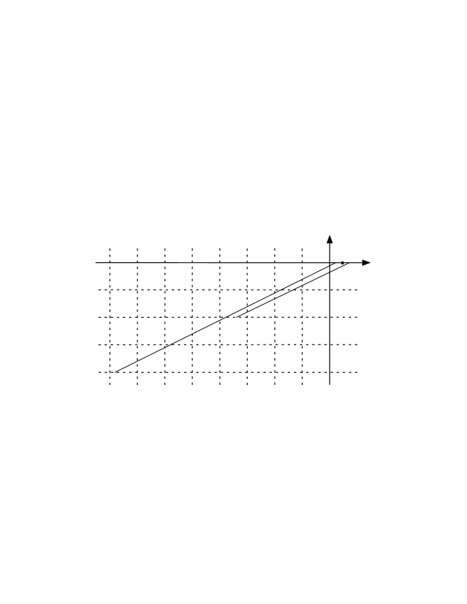
$R_{2}$
                                    $R_{1}$

Figure 9: $+\frac{1}{2}$ surgery on $K(2,5)$

Theorem 6.12.

Suppose $1\leq\ell\leq(q-1)/2$ and let $C_{t}$ be a path of flat reducible connections on $Z$ in normal form such that ${C_{t}}|_{T}=\frac{t+\ell-1}{q}idx$ for $t\in[0,1]$. Notice that $C_{t}$ crosses one and only one ${\mathbb{C}}^{2}$ jumping point (the one at $\frac{2\ell-1}{2q}$). Then

$$SF(C_{t};Z;P^{-})=2.$$

ProofFirst notice that $-2\leq SF(C_{t};Z;P^{-})\leq 2$. This is because the kernel of $D_{C_{t}}$ on $Z$ with $P^{-}$ boundary conditions is $2$–dimensional at the jumping points, and $0$–dimensional at non-trivial reducible connections. Thus two eigenvalues become zero at the jumping point.

We prove the theorem by comparing the rho invariant for gauge equivalent flat connections on the manifold $X_{+1}$ obtained by $+1$ surgery on $K(2,q)$.

The path

$$R_{1}(t)=(1-t)(\tfrac{1}{4q},0)+t(\tfrac{1}{2}-\tfrac{1}{4q}+1-q,1-q)$$

(see Proposition 6.8) crosses the vertical axis at $t_{0}=\frac{1}{(q-1)(4q-2)}$. Let $(m_{t},n_{t})$ be the composition of the short horizontal segment from $(0,0)$ to $(\frac{1}{4q},0)$ with the path $R_{1}(t)$ for $0\leq t\leq t_{0}$ and let $A_{t}$ be the path of connections on $X_{+1}$ which are flat along $Z$ and correspond to the path $(m_{t},n_{t})$ by the construction of Subsection 5.1 of $X_{+1}$. From this path, we compute that $a=0,b=-1,c=0$ and that $2\int m^{\prime}n=\frac{1}{4q(4q-2)}.$ Since $A_{t}$ misses all the ${\mathbb{C}}^{2}$ jumping points, $SF(A_{t};Z;P^{-})=0$ and Theorem 5.7 implies

$$\varrho_{X_{+1}}(A_{1}) = 4(a-b+c)-2-8\int m^{\prime}n$$

$$= 2-\frac{1}{q(4q-2)}.$$

Now consider the path obtained by translating $R_{1}(t)$ by the vector $(q-1,q-1)$. Proposition 6.8 implies that this is another lift to ${\mathbb{R}}^{2}$ of the arc $\widehat{R}_{1}\subset{\mathfrak{R}}^{*}_{SU(2)}(Z)$. Parameterized in the opposite direction (so that it starts on the horizontal axis), this is the curve

$$\widetilde{R}(t)=(1-t)(\tfrac{1}{2}-\tfrac{1}{4q},0)+t(\tfrac{1}{4q}+q-1,q-1).$$

This crosses the vertical line $x=q-1$ when $\tilde{t}_{0}=1-t_{0}=\frac{4q^{2}-6q+1}{4q^{2}-6q+2}$. Let $(\tilde{m}_{t},\tilde{n}_{t})$ be the composition of the short horizontal segment from $(0,0)$ to $(\frac{1}{2}-\frac{1}{4q},0)$ with $\widetilde{R}(t)$ for $0\leq t\leq\tilde{t}_{0}.$ The corresponding path $\widetilde{A}_{t}$ of connections crosses each of the ${\mathbb{C}}^{2}$ jumping points exactly once and ends at $\widetilde{A}_{1}$, which is gauge equivalent to $A_{1}.$ Using the path, we compute as before that $\tilde{a}=q-1$ and $\tilde{b}=q-2$. To compute $\tilde{c}$, observe that $\widetilde{R}(t)$ intersects the horizontal line $y=i$ in the point $(x_{i},i)$ with $i<x_{i}<i+1$ if $i=1,\cdots,q-1$. Thus the loop constructed in Subsection 5.1 encloses no lattice points of the form $(1,n)$, one lattice point of the form $(2,n)$ (namely $(2,1)$), and in general encloses $j-1$ lattice points of the form $(j,n)$. Hence in total, the loop encloses $1+2+\cdots+(q-2)=\tfrac{(q-2)(q-1)}{2}$ lattice points. These are all enclosed clockwise, so $\tilde{c}=\tfrac{(q-2)(q-1)}{2}=q^{2}-3q+2$.

The integral $2\int m^{\prime}n$ is equal to $\frac{(4q^{2}-6q+1)^{2}}{4q(4q-2)}.$ Hence

$$\varrho_{X_{+1}}(\widetilde{A}_{1}) = 4(\tilde{a}-\tilde{b}+\tilde{c})-2-8\int m^{\prime}n+2SF(\widetilde{A}_{t};Z;P^{-})$$

$$= 4-2q-\frac{1}{q(4q-2)}+2SF(\widetilde{A}_{t};Z;P^{-}).$$

Since $A_{1}$ and $\widetilde{A}_{1}$ are gauge equivalent, their rho invariants are equal. Setting $\varrho_{X_{+1}}(A_{1})=\varrho_{X_{+1}}(\widetilde{A}_{1})$ and solving for $SF(\widetilde{A}_{t};Z;P^{-})$ gives

$$SF(\widetilde{A}_{t};Z;P^{-})=q-1.$$

Since there are exactly $\frac{q-1}{2}$ ${\mathbb{C}}^{2}$–jumping points, the path $\widetilde{A}_{t}$ passes through all of them, and each contributes at most $2$ to the spectral flow, the spectral flow across each one is $2.$ This proves the theorem.

The following lemma will be useful in simplifying formulas.

Lemma 6.13.

Let $q,k,\ell,i$ be positive integers with $q\geq 3$, $\ell\leq\frac{q-1}{2}$, and $i\leq k(q-2\ell+1)$. Let $[x]$ be the greatest integer less than or equal to $x.$ Then

$$\left[\frac{4q(1-i)-2\ell+1}{4qk-2}\right]=\left[-\frac{i}{k}\right]=\left[\frac{2\ell-4qi-1}{4qk+2}\right].$$

ProofLetting $x=\tfrac{4q(1-i)-2\ell+1}{4qk-2}$, one can easily check that $0<x+\tfrac{i}{k}<\tfrac{1}{k}$. This implies that $[x]=[-\tfrac{i}{k}]$. Similarly, letting $y=\tfrac{2\ell-4qi-1}{4qk+2}$, one checks that $0<y+\tfrac{i}{k}<\tfrac{1}{k}$, which implies $[y]=[-\tfrac{i}{k}]$.

We can now turn our attention to computing the gauge theoretic invariants. Suppose $k>0$ and let $X_{\pm k}$ denote the manifold obtained by $\pm\frac{1}{k}$ surgery on $K(2,q).$ By Proposition 6.8, the curves

$$R_{\ell}(t)=(1-t)\left(\tfrac{2\ell-1}{4q},0\right)+t\left(\tfrac{1}{2}-\tfrac{2\ell-1}{4q}\pm k(2\ell-q-1),\,2\ell-q-1\right),\ \ 0<t<1$$

for $\ell=1,\ldots,(q-1)/2$ are lifts of the restrition map ${\mathfrak{R}}^{*}_{SU(2)}(Z)\longrightarrow{\mathfrak{R}}_{SU(2)}(T)$ under the branched cover $f_{\pm k}\co{\mathbb{R}}^{2}\longrightarrow{\mathfrak{R}}_{SU(2)}(T)$.

Consider first the case of positive surgeries. We would like to determine the flat connections which extend over $X_{k}$ for $k>0.$ Fixing $\ell,$ these correspond to points on $R_{\ell}(t)$ whose first coordinate is an integer. This happens when

$$t_{i}=\frac{4q(1-i)-2\ell+1}{(4qk-2)(2\ell-q-1)},$$

in which case the first coordinate of $R_{\ell}(t)$ is $1-i$, with $i\in\{1,\ldots,k(q-2\ell+1)\}$.

Fix $\ell$ and $i$ with $1\leq\ell\leq\frac{q-1}{2}$ and $1\leq i\leq k(q-2\ell+1)$. Define the path $(m_{t},n_{t})$ to be the composition of the horizontal line segment from $(0,0)$ to $(\tfrac{2\ell-1}{4q},0)$ with the path $R_{\ell}(t)$ for $t\in[0,t_{i}]$. Let $A_{t}$ be the path of connections corresponding to $(m_{t},n_{t})$ by the construction of Subsection 5.1. The endpoint, which we denote by $A_{\ell,i},$ extends flatly over $X_{k}$. Denote the integers $a,\ b,\ c$ associated to $A_{\ell,i}$ by $a_{\ell,i},\ b_{\ell,i},\ c_{\ell,i}$. Then, using Lemma 6.13 one sees that

$$a_{\ell,i} = m_{t_{i}}=1-i$$

$$b_{\ell,i} = [n_{t_{i}}]=[t_{i}(2\ell-q-1)]=\left[\frac{4q(1-i)-2\ell+1}{4qk-2}\right]=\left[-\frac{i}{k}\right].$$

Inspecting the graph of $(m_{t},n_{t})$ one sees that $c_{\ell,i}-c_{\ell,i-1}=2(-b_{\ell,i-1})$ and $c_{\ell,1}=0$, so

$$c_{\ell,i}=-2\sum_{j<i}b_{\ell,j}=-2\sum_{j=1}^{i-1}\left[-\frac{j}{k}\right].$$

To calculate the Chern–Simons invariant, we compute the integral:

$$2\int m^{\prime}n = 2\int_{0}^{t_{i}}[(k-\tfrac{1}{2q})(2\ell-q-1)](2\ell-q-1)t\ dt$$

$$= \frac{(4q(1-i)-2\ell+1)^{2}}{4q(4qk-2)}.$$

Since the horizontal line segment from $(0,0)$ to $(\tfrac{2\ell-1}{4q},0)$ (ie, the first part of the path) passes through the ${\mathbb{C}}^{2}$ jumping points at $\tfrac{1}{2q},\tfrac{3}{2q},\cdots,\tfrac{2[\ell/2]-1}{2q}$, Theorem 6.12 implies that $SF(C_{t};Z;P^{-})=2[\tfrac{\ell}{2}]$.

Applying Theorems 5.4, 5.5 and 5.7, we compute the spectral flow, the Chern–Simons invariants and the rho invariants of $A_{\ell,i}$. The results are summarized in the following theorem.

Theorem 6.14.

Suppose $k>0$ and let $X_{k}$ be the result of $\frac{1}{k}$ surgery on the $(2,q)$ torus knot. Let $A_{\ell,i}$ for $\ell=1,\ldots,{(q-1)}/{2}$ and $i=1,\ldots,k(q+1-2\ell)$ be the flat connections on $X_{k}$ constructed above. Then

$$SF(\Theta,A_{\ell,i};X_{k}) = 2\left[\frac{\ell}{2}\right]-2i-2\left[-\frac{i}{k}\right]$$

$$cs(A_{\ell,i}) = \frac{(4q(1-i)-2\ell+1)^{2}}{4q(4qk-2)}+2\sum_{j=1}^{i-1}\left[-\frac{j}{k}\right]$$

$$\varrho_{X_{k}}(A_{\ell,i}) = 4\left[\frac{\ell}{2}\right]+2-4i-\frac{(4q(1-i)-2\ell+1)^{2}}{q(4qk-2)}$$

$$-4\left[-\frac{i}{k}\right]-8\sum_{j=1}^{i-1}\left[-\frac{j}{k}\right].$$

Now consider the situation for negative surgeries on $K(2,q)$. We would like to determine the flat connections which extend over $X_{-k}$. (To make counting arguments simpler we still assume $k>0$). Fixing $\ell,$ these correspond to points on $R_{\ell}(t)$ whose first coordinate is an integer. This happens when

$$t_{i}=\frac{4qi-2\ell+1}{(q-2\ell+1)(4qk+2)},$$

in which case the first coordinate of $R_{\ell}(t)$ is $i$, with $i\in\{1,\ldots,k(q-2\ell+1)\}$.

Fix $\ell$ and $i$ with $1\leq\ell\leq(q-1)/2$ and $1\leq i\leq k(q-2\ell+1).$ Define the path $(m_{t},n_{t})$ to be the composition of the horizontal line from $(0,0)$ to $(\frac{2\ell-1}{4q},0)$ with $R_{\ell}(t)$ for $t\in[0,t_{i}].$ Let $A_{t}$ be the path of connections corresponding to $(m_{t},n_{t})$ by the construction of Subsection 5.1. The endpoint, which we denote by $A_{\ell,i},$ extends flatly over $X_{-k}$. We compute the numbers $a_{\ell,i},\ b_{\ell,i},\ c_{\ell,i}$ associated to $A_{\ell,i}$. First,

$$a_{\ell,i} = m_{t_{i}}=i$$

$$b_{\ell,i} = [n_{t_{i}}]=[t_{i}(2\ell-q-1)]=\left[\frac{2\ell-4qi-1}{4qk+2}\right]=\left[-\frac{i}{k}\right]$$

using Lemma 6.13. Inspecting the graph of $(m_{t},n_{t})$ one sees that

$$c_{\ell,i}=2\sum_{j\leq i}b_{\ell,j}=2\sum_{j=1}^{i}\left[-\frac{j}{k}\right].$$

Finally,

$$2\int_{0}^{t_{i}}m^{\prime}n=-\frac{(4qi-2\ell+1)^{2}}{4q(4qk+2)}.$$

Just as in the case of positive surgery, the first part of the path passes through the ${\mathbb{C}}^{2}$ jumping points at $\tfrac{1}{2q},\tfrac{3}{2q},\cdots,\tfrac{2[\ell/2]-1}{2q}$ and thus $SF(C_{t};Z;P^{-})=2[\tfrac{\ell}{2}]$.

Theorems 5.4, 5.5 and 5.7 then give formulas for the spectral flow, the Chern–Simons invariants, and the rho invariants for all connections on $X_{-k}$.

Theorem 6.15.

Suppose $k>0$ and let $X_{-k}$ be the result of $-\frac{1}{k}$ surgery on the $(2,q)$ torus knot. Let $A_{\ell,i}$ for $\ell=1,\ldots,\frac{q-1}{2}$ and $i=1,\ldots,k(q+1-2\ell)$ be the flat connections constructed above. Then

$$SF(\Theta,A_{\ell,i};X_{-k}) = 2\left[\frac{\ell}{2}\right]+2i-2-2\left[-\frac{i}{k}\right]$$

$$cs(A_{\ell,i}) = -\frac{(4qi-2\ell+1)^{2}}{4q(4qk+2)}-2\sum_{j=1}^{i}\left[-\frac{j}{k}\right]$$

$$\varrho_{X_{-k}}(A_{\ell,i}) = 4\left[\frac{\ell}{2}\right]-2+4i+\frac{(4qi-2\ell+1)^{2}}{q(4qk+2)}$$

$$-4\left[-\frac{i}{k}\right]+8\sum_{j=1}^{i}\left[-\frac{j}{k}\right].$$

Summing the rho invariants and applying Theorem 6.7 yields the correction term $\lambda^{\prime\prime}_{SU(3)}$ for any homology sphere obtained by surgeries on a $(2,q)$ torus knot. The results are summarized in Table 3. (The computations of $\lambda^{\prime}_{SU(3)}$ can be found in [4].)

$$\begin{array}[]{|c|cc|}\hline\cr&\lambda^{\prime}_{SU(3)}(X_{k})&\lambda^{\prime\prime}_{SU(3)}(X_{k})\\ \hline\cr\ K(2,3)&3k^{2}-k&{\displaystyle\frac{-24k^{3}-84k^{2}+13k}{6(6k-1)}}\\ \ K(2,5)&33k^{2}-9k&{\displaystyle\frac{-200k^{3}-1620k^{2}+151k}{10(10k-1)}}\\ \ K(2,7)&138k^{2}-26k&{\displaystyle\frac{-784k^{3}-9128k^{2}+606k}{14(14k-1)}}\\ \ K(2,9)&\ 390k^{2}-58k&\ {\displaystyle\frac{-2160k^{3}-33192k^{2}+1714k}{18(18k-1)}}\\ \hline\cr\end{array}$$

Table 3: $\lambda^{\prime}_{SU(3)}$ and $\lambda^{\prime\prime}_{SU(3)}$ for homology spheres $X_{k}$ obtained by $\tfrac{1}{k}$ surgery on $K(2,q)$

In completing this table we used the following fact. Fix $q$ and let $X_{k}$ denote the manifold obtained by $\tfrac{1}{k}$ surgery on $K(2,q)$. As noted after the proof of Theorem 6.11, for positive $k$ the quantity $2q(2q-1)\lambda^{\prime\prime}_{SU(3)}(X_{k})$ is a cubic polynomial in $k$. Hence one can deduce $\lambda^{\prime\prime}_{SU(3)}(X_{k})$ for all $k$ by computing it in several examples and solving for the coefficients. Similar methods apply if $k$ is negative.

The entries in this table are valid for any integer $k$, not just $k>0$. Despite the slight differences in the statements and proofs of Theorems 6.14 and 6.15, after summing over all $A_{i}$, the resulting formulas give the same rational function. For $k=0$ the homology sphere is $S^{3}$ which has $SU(3)$ Casson invariant $0$ since it is simply connected.

By summing $\lambda^{\prime}_{SU(3)}$ and $\lambda^{\prime\prime}_{SU(3)},$ we compute the $SU(3)$ Casson invariants for homology 3–spheres $X_{k}$ obtained by $\tfrac{1}{k}$ surgery on $K(2,q)$.

$$\begin{array}[]{|c|c|}\hline\cr&\lambda_{SU(3)}(X_{k})\\ \hline\cr\ K(2,3)&{\displaystyle\frac{84k^{3}-138k^{2}+19k}{6(6k-1)}}\\ \ K(2,5)&{\displaystyle\frac{3100k^{3}-2850k^{2}+241k}{10(10k-1)}}\\ \ K(2,7)&{\displaystyle\frac{26264k^{3}-16156k^{2}+970k}{14(14k-1)}}\\ \ K(2,9)&\ {\displaystyle\frac{124200k^{3}-59004k^{2}+2758k}{18(18k-1)}}\\ \hline\cr\end{array}$$

Table 4: The $SU(3)$ Casson invariants for homology spheres $X_{k}$ obtained by $\tfrac{1}{k}$ surgery on $K(2,q)$

As remarked above, for $k>0$, $\pm\tfrac{1}{k}$ surgery on $K(2,q)$ is homeomorphic to the Brieskorn sphere $\Sigma(2,q,2qk\mp 1)$ up to a possible change of orientations. However, $\lambda_{SU(3)}$ does not depend on the choice of orientation. Thus Table 4 also gives the $SU(3)$ Casson invariants of $\Sigma(2,q,2qk\pm 1)$ for $q=3$, $5$, $7$, and $9$.

From this data we conclude that $\lambda_{SU(3)}$ is not a finite type invariant of low order.

Theorem 6.16.

$\lambda_{SU(3)}$ is not a finite type invariant of order $\leq 6$.

ProofWe argue by contradiction. Suppose $\lambda_{SU(3)}$ is a finite type invariant of order $\leq 6$. Since $\lambda_{SU(3)}(S^{3})=0$ and since it is invariant under change of orientation, it follows that there exist constants $A$ and $B$ such that

$$\lambda_{SU(3)}=A(\lambda_{2}+12\lambda_{SU(2)})+B\lambda_{SU(2)}^{2},$$ (6.7)

where $\lambda_{2}$ is the second Ohtsuki invariant [27] and $\lambda_{SU(2)}$ is Casson’s invariant [1]. Both of these invariants satisfy surgery formulas (see Theorem 4.3 in [27] for $\lambda_{2}$) and so can be computed in all the examples considered here. If Equation (6.7) were true, then each one of our computations would provide a linear constraint on $A$ and $B$. But just from surgeries on the trefoil, it follows that no such $A$ and $B$ exist. Thus $\lambda_{SU(3)}$ is not an invariant of finite type of order $\leq 6.$

RemarkStavros Garoufalidis has observed that our computations here prove that $\lambda_{SU(3)}$ is not a finite type invariant of any order.

6.5 Concluding remarks and open problems

The methods we have developed apply more generally than these computations suggest. For example, although we have restricted our attention to homology spheres obtained from surgeries on the $(2,q)$ torus knots, the same methods apply to any Seifert fibered homology sphere. For example, although $\Sigma(2,5,7)$ is not obtained by surgery on a torus knot in $S^{3},$ it can be described as surgery on a torus-like knot in a homology sphere to which our main results apply. More generally, one can compute the ${\mathbb{C}}^{2}$–spectral flow, the Chern–Simons invariants and the rho invariants for Brieskorn homology spheres. From this, one can deduce their $SU(3)$ Casson invariants in case $p=2.$ On the other hand, computing $\lambda_{SU(3)}(\Sigma(p,q,r))$ when $p,q,r>2$ requires the use of perturbations and goes beyond the scope this article. This problem will be addressed in a later article.

Our methods can also be used to compute $\lambda_{SU(3)}$ for Dehn surgeries on knots other than torus knots, eg, the figure eight knot. The idea is to first notice that one of the surgeries on the figure eight knot gives $\Sigma(2,3,7)$. This manifold can then be used as a reference point from which to calculate the invariants for other surgeries. This is especially interesting since most of the homology spheres obtained from surgery on the figure eight knot are hyperbolic. The crucial point in making this idea work is that our formula for splitting the spectral flow and the subsequent applications do not assume the path $C_{t}$ of connections on $Z$ is flat.

In another direction, our technique for computing gauge theoretic invariants can be generalized to groups other than $SU(2)$ and representations other than ${\mathbb{C}}^{2}$. For example, one can adapt our approach to compute the ${\rm ad}\ su(2)$–spectral flow which arises in Floer’s instanton homology and in asymptotic expansions of Witten’s 3–manifold invariants (see [20]).

One interesting and difficult problem is to determine the extent to which the Atiyah–Patodi–Singer rho invariants fail to be invariant under homotopy equivalence. The results of [15] show that the rho invariants of homotopy equivalent manifolds differ by a locally constant function on the representation variety. The cut–and–paste methods introduced here give a technique to compute this difference on the various path components of the representation variety. We plan to pursue this question in a future work.

In closing, we would like to mention one final interesting problem raised by our results. Although $\lambda_{SU(3)}$ is not a finite type invariant, it may still be possible to express some of the coefficients of the cubic polynomials in the numerators of $\lambda_{SU(3)}(X_{k})$ in Table 4 in terms of the Alexander or Jones knot polynomials of the corresponding knot. For this problem, note that the denominators $2q(2qk\pm 1)$ appearing in Table 4 are just the denominators of the Chern–Simons invariants of $\Sigma(2,q,2qk\pm 1)$. We do not know if the Chern–Simons invariants are rational for general homology spheres, or, alternatively, if the quantity $pq(pqk\mp 1)$ associated to $\pm\frac{1}{k}$ surgery on $K(p,q)$ extends naturally to define an invariant for all homology spheres.

References

- [1] S Akbulut, J McCarthy, Casson’s invariant for oriented homology 3–spheres, an exposition, Mathematical Notes no. 36, Princeton University Press (1990)
- [2] D Auckly, A topological method to compute spectral flow, Kyungpook Math. J. 38 (1998) 181–203
- [3] M F Atiyah, V K Patodi, I M Singer, Spectral asymmetry and Riemannian geometry. I,II,III, Math. Proc. Camb. Phil. Soc. 77 (1975) 43–69; 78 (1975) 405–432; 79 (1976) 71–99
- [4] H U Boden, Unitary representations of Brieskorn spheres, Duke J. Math. 75 (1994) 193–220
- [5] H U Boden, C M Herald, The SU(3) Casson invariant for integral homology 3–spheres, J. Diff. Geom. 50 (1998) 147–206
- [6] B Booss-Bavnbek, K Wojciechowski, Elliptic Boundary Problems for Dirac Operators, Birkhäuser, Boston (1993)
- [7] U Bunke, On the gluing problem for the -invariant, J. Diff. Geom. 41 (1995) 397-448
- [8] S Cappell, R Lee, E Miller, A symplectic geometry approach to generalized Casson’s invariant, Bull. Amer. Math. Soc. 22 (1990) 269–275
- [9] S Cappell, R Lee, E Miller, On the Maslov index, Comm. Pure Appl. Math. 47 (1994) 121–186
- [10] S Cappell, R Lee, E Miller Self-adjoint elliptic operators and manifold decompositions: I. Low eigenmodes and stretching, Comm. Pure Appl. Math. 49 (1996) 825–866; II. Spectral flow and Maslov index, 49 (1996) 869–909
- [11] H S M Coxeter, W O Moser, Generators and Relations for Discrete Groups, 2nd edition, Ergeb. u. Ihrer Grenz. Springer–Verlag, New York (1965)
- [12] M Daniel, An extension of a theorem of Nicolaescu on spectral flow and the Maslov index, Proc. Amer. Math. Soc. 128 (2000) 611–619
- [13] M Daniel, Maslov index, symplectic reduction in a symplectic Hilbert space and a splitting formula for spectral flow, PhD Thesis, Indiana University, Bloomington, 1997
- [14] M Daniel, P Kirk, A general splitting theorem for spectral flow, with an appendix by K P Wojciechowski, Michigan Math. J. 46 (1999) 589–617
- [15] M Farber, J Levine, Jumps of the eta-invariant. With an appendix by S Weinberger: Rationality of –invariants. Math. Zeit. 223 (1996) 197–246
- [16] B Fine, P Kirk, E Klassen, A local analytic splitting of the holonomy map on flat connections, Math. Ann. 299 (1994) 171–189
- [17] R Fintushel, R Stern, Instanton homology of Seifert-fibered 3–spheres, Proc. Lond. Math. Soc. (3) 61 (1990) 109–138
- [18] T Kato, Perturbation Theory of Linear Operators, 2nd edition, Grund. der math. Wissen. 132, Springer, Berlin (1980)
- [19] P Kirk, E Klassen, Chern–Simons invariants of 3–manifolds and representation spaces of knot groups, Math. Ann. 287 (1990) 347–367
- [20] P Kirk, E Klassen, Computing spectral flow via cup products, J. Diff. Geom. 40 (1994) 505–562
- [21] P Kirk, E Klassen, Analytic deformations of the spectrum of a family of Dirac operators on an odd-dimensional manifold with boundary, Mem. Amer. Math. Soc. 124 (1996) no. 592
- [22] P Kirk, E Klassen, The spectral flow of the odd signature operator and higher Massey products, Math. Proc. Camb. Phil. Soc. 121 (1997) 297–320
- [23] P Kirk, E Klassen, Continuity and analyticity of families of self-adjoint Dirac operators on a manifold with boundary, Illinois J. Math. 42 (1998) 123–138
- [24] P Kirk, E Klassen, D Ruberman, Splitting the spectral flow and the Alexander matrix, Comm. Math. Helv. 69 (1994) 375–416
- [25] P Kirk, M Lesch, The eta-invariant, Maslov index, and spectral flow for Dirac-type operators on manifolds with boundary, preprint (2000) arxiv:math.DG/0012123
- [26] E Klassen, Representations of knot groups in SU(2), Trans. Amer. Math. Soc. 326 (1991) 795–828
- [27] X-S Lin, Z Wang, Fermat limit and congruence of Ohtsuki invariants, from: “Proceedings of the Kirbyfest (Berkeley, CA, 1998)”, Geometry and Topology Monographs 2 (1999) 321–333
- [28] T Mrowka, K Walker, private communication of unpublished research (1993)
- [29] L Nicolaescu, The Maslov index, the spectral flow, and splittings of manifolds, Duke Math. J. 80 (1995) 485–533
- [30] L Nicolaescu, Generalized symplectic geometries and the index of families of elliptic problems, Mem. Amer. Math. Soc. 126 (1997) no. 609
- [31] C Taubes, Casson’s invariant and gauge theory, J. Diff. Geom. 31 (1990) 547–599
- [32] K Walker, An extension of Casson’s invariant, Annals of Math Studies 126, Princeton University Press (1992)