Fast and accurate multigrid solution of Poissons equation using diagonally oriented grids
Abstract
We solve Poisson’s equation using new multigrid algorithms that converge rapidly. The novel feature of the 2D and 3D algorithms are the use of extra diagonal grids in the multigrid hierarchy for a much richer and effective communication between the levels of the multigrid. Numerical experiments solving Poisson’s equation in the unit square and unit cube show simple versions of the proposed algorithms are up to twice as fast as correspondingly simple multigrid iterations on a conventional hierarchy of grids.
1 Introduction
Multigrid algorithms are effective in the solution of elliptic problems and have found many applications, especially in fluid mechanics [6, e.g.], chemical reactions in flows [8, e.g.] and flows in porous media [7]. Typically, errors in a solution may decrease by a factor of 0.1 each iteration [5, e.g.]. The simple algorithms I present decrease errors by a factor of (see Tables 1 and 3 on pages 1 and 3). Further gains in the rate of convergence may be made by further research.
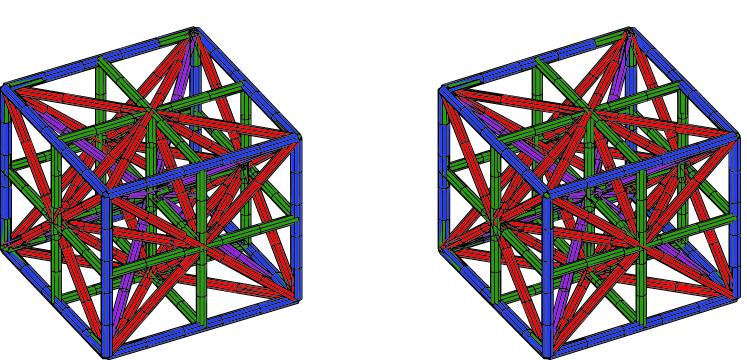
Conventional multigrid algorithms use a hierarchy of grids whose grid spacings are all proportional to where is the level of the grid [9, e.g.]. The promising possibility I report on here is the use of a richer hierarchy of grids with levels of the grids oriented diagonally to other levels. Specifically, in 2D I introduce in Section 2 a hierarchy of grids with grid spacings proportional to and with grids aligned at to adjacent levels, see Figure 1 (p1).111This paper is best viewed and printed in colour as the grid diagrams and the ensuing discussions are all colour coded. In 3D the geometry of the grids is much more complicated. In Section 3 we introduce and analyse a hierarchy of 3D grids with grid spacings roughly on the different levels, see Figure 4 (p4). Now Laplace’s operator is isotropic so that its discretisation is straightforward on these diagonally oriented grids. Thus in this initial work I explore only the solution of Poisson’s equation.
| (1) |
Given an approximation to a solution, each complete iteration of a multigrid scheme seek a correction so that is a better approximation to a solution of Poisson’s equation (1). Consequently the update has to approximately satisfy a Poisson’s equation itself, namely
| (2) |
is the residual of the current approximation. The multigrid algorithms aim to estimate the error as accurately as possible from the residual . Accuracy in the ultimate solution is determined by the accuracy of the spatial discretisation in the computation of the residual : here we investigate second-order and fourth-order accurate discretisations [9, e.g.] but so far only find remarkably rapid convergence for second-order discretisations.
The diagonal grids employed here are perhaps an alternative to the semi-coarsening hierarchy of multigrids used by Dendy [1] in more difficult problems.
In this initial research we only examine the simplest reasonable V-cycle on the special hierarchy of grids and use only one Jacobi iteration on each grid. We find in Sections 2.1 and 3.1 that the smoothing restriction step from one grid to the coarser diagonally orientated grid is done quite simply. Yet the effective smoothing operator from one level to that a factor of 2 coarser, being the convolution of two or three intermediate steps, is relatively sophisticated. One saving in using these diagonally orientated grids is that there is no need to do any interpolation. Thus the transfer of information from a coarser to a finer grid only involves the simple Jacobi iterations described in Sections 2.2 and 3.2. Performance is enhanced within this class of simple multigrid algorithms by a little over relaxation in the Jacobi iteration as found in Sections 2.4 and 3.4. The proposed multigrid algorithms are found to be up to twice as fast as comparably simple conventional multigrid algorithms.
2 A diagonal multigrid for the 2D Poisson equation
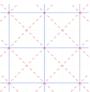
To approximately solve Poisson’s equation (2) in two-dimensions we use a novel hierarchy of grids in the multigrid method. The length scales of the grid are . If the finest grid is aligned with the coordinate axes with grid spacing say, the first coarser grid is at with spacing , the second coarser is once again aligned with the axes and of spacing , as shown in Figure 1, and so on for all other levels on the multigrid. In going from one level to the next coarser level the number of grid points halves.
2.1 The smoothing restriction
The restriction operator smoothing the residual from one grid to the next coarser grid is the same at all levels. It is simply a weighted average of the grid point and the four nearest neighbours on the finer grid as shown in Figure 2. To restrict from a fine green grid to the diagonal red grid
| (3) |
whereas to restrict from a diagonal red grid to the coarser blue grid
| (4) |
Each of these restrictions takes per grid element. Thus assuming the finest grid is with grid points, the restriction to the next finer diagonal grid (red) takes approximately , the restriction to the next finer takes approximately , etc. Thus to restrict the residuals up levels to the coarsest grid spacing of takes
| (5) |
In contrast a conventional nine point restriction operator from one level to another takes per grid point, which then totals to approximately over the whole conventional multigrid hierarchy. This is somewhat better than the proposed scheme, but we make gains elsewhere. In restricting from the green grid to the blue grid, via the diagonal red grid, the restriction operation is equivalent to a 17-point stencil with a much richer and more effective smoothing than the conventional 9-point stencil.
2.2 The Jacobi prolongation
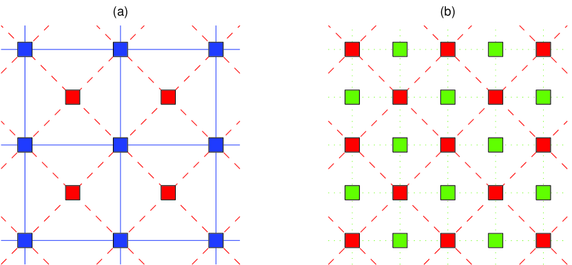
One immediate saving is that there is no need to interpolate in the prolongation step from one level to the next finer level. For example, to prolongate from the blue grid to the finer diagonal red grid, shown in Figure 3(a), estimate the new value of at the red grid points on level by the red-Jacobi iteration
| (6) |
when the grid spacing on the red grid is . Then the values at the blue grid points are refined by the blue-Jacobi iteration
| (7) |
A similar green-red Jacobi iteration will implicitly prolongate from the red grid to the finer green grid shown in Figure 3(b). These prolongation-iteration steps take per grid point. Thus to go from the red to the green grid takes . As each level of the grid has half as many grid points as the next finer, the total operation count for the prolongation over the hierarchy from grid spacing is
| (8) |
The simplest (bilinear) conventional interpolation direct from the blue grid to the green grid would take approximately , to be followed by for a Jacobi iteration on the fine green grid (using simply and ). Over the whole hierarchy this takes approximately . This is a little smaller than that proposed here, but the proposed diagonal method achieves virtually two Jacobi iterations instead of just one and so is more effective.
2.3 The V-cycle converges rapidly
Numerical experiments show that although the operation count of the proposed algorithm is a little higher than the simplest usual multigrid scheme, the speed of convergence is much better. The algorithm performs remarkably well on test problems such as those in Gupta et al [2]. I report a quantitative comparison between the algorithms that show the diagonal scheme proposed here is about twice as fast.
Both the diagonal and usual multigrid algorithms use to compute the residuals on the finest grid. Thus the proposed method takes approximately per V-cycle of the multigrid iteration, although 17% more than the simplest conventional algorithm that takes , the convergence is much faster. Table 1 shows the rate of convergence for this diagonal multigrid based algorithm. The data is determined using matlab’s sparse eigenvalue routine to find the largest eigenvalue and hence the slowest decay on a grid. This should be more accurate than limited analytical methods such as a bi-grid analysis [3]. Compared with correspondingly simple schemes based upon the usual hierarchy of grids, the method proposed here takes much fewer iterations, even though each iteration is a little more expensive, and so should be about twice as fast.
| algorithm | per iter | per dig | per dig | |||
|---|---|---|---|---|---|---|
| diagonal, | .099 | 1.052 | .052 | |||
| usual, | .340 | 1.121 | .260 | |||
| diagonal, | .333 | 1.200 | .200 | |||
| usual, | .343 | 1.216 | .216 |
Fourth-order accurate solvers in space may be obtained using the above second-order accurate V-cycle as done by Iyengar & Goyal [4]. The only necessary change is to compute the residual in (2) on the finest grid with a fourth-order accurate scheme, such as the compact “Mehrstellen” scheme
| (9) | |||||
Use the V-cycles described above to determine an approximate correction to the field based upon these more accurate residuals. The operation count is solely increased by the increased computation in the residual, from per iteration to (the combination of appearing on the right-hand side of (9) need not be computed each iteration). Numerical experiments summarised in Table 1 show that the multigrid methods still converge, but the diagonal method has lost its advantages. Thus fourth order accurate solutions to Poisson’s equation are most quickly obtained by initially using the diagonal multigrid method applied to the second order accurate computation of residuals. Then use a few multigrid iterations based upon the fourth order residuals to refine the numerical solution.
2.4 Optimise parameters of the V-cycle
The multigrid iteration is improved by introducing a small amount of over relaxation.
First we considered the multigrid method applied to the second-order accurate residuals. Numerical optimisation over a range of introduced parameter values suggested that the simplest, most robust effective change was simply to introduce a parameter into the Jacobi iterations (6–7) to become
| (10) | |||||
| (11) |
on a diagonal red grid and similarly for a green grid. An optimal value of was determined to be . The parameter just increases the weight of the residuals at each level by about 5%. This simple change, which does not increase the operation count, improves the factor of convergence to , which decreases the necessary number of iterations to achieve a given accuracy. As Table 1 shows, this diagonal multigrid is still far better than the usual multigrid even with its optimal choice for over relaxation.
Then we considered the multigrid method applied to the fourth-order accurate residuals. Numerical optimisation of the parameter in (10–11) suggests that significantly more relaxation is preferable, namely . With this one V-cycle of the multigrid method generally reduces the residuals by a factor . This simple refinement reduces the number of iterations required by about one-third in converging to the fourth-order accurate solution.
3 A diagonal multigrid for the 3D Poisson equation
The hierarchy of grids we propose for solving Poisson’s equation (2) in three-dimensions is significantly more complicated than that in two-dimensions. Figure 4 shows the three steps between levels that will be taken to go from a fine standard grid (green) of spacing , via two intermediate grids (red and magenta), to a coarser regular grid (blue) of spacing . As we shall discuss below, there is some unevenness in the hierarchy that needs special treatment.
3.1 The smoothing restriction steps
The restriction operation in averaging the residuals from one grid to the next coarser grid is reasonably straightforward.
-
•
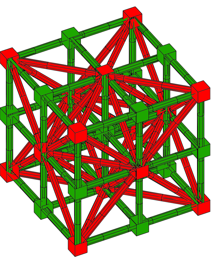
Figure 5: the green and red grids superimposed showing the nodes of the red grid at the corners and faces of the cube, and their relationship to their six neighbouring nodes on the finer green grid. The nodes of the red grid are at the corners of the cube and the centre of each of the faces as seen in Figure 5. They each have six neighbours on the green grid so the natural restriction averaging of the residuals onto the red grid is
(12) for corresponding to the (red) corners and faces of the coarse (blue) grid. When the fine green grid is so that there are unknowns on the fine green grid, this average takes for each of the approximately red nodes. This operation count totals .
Note that throughout this discussion of restriction from the green to blue grids via the red and magenta, we index variables using subscripts appropriate to the fine green grid. This also holds for the subsequent discussion of the prolongation from blue to green grids.
-
•
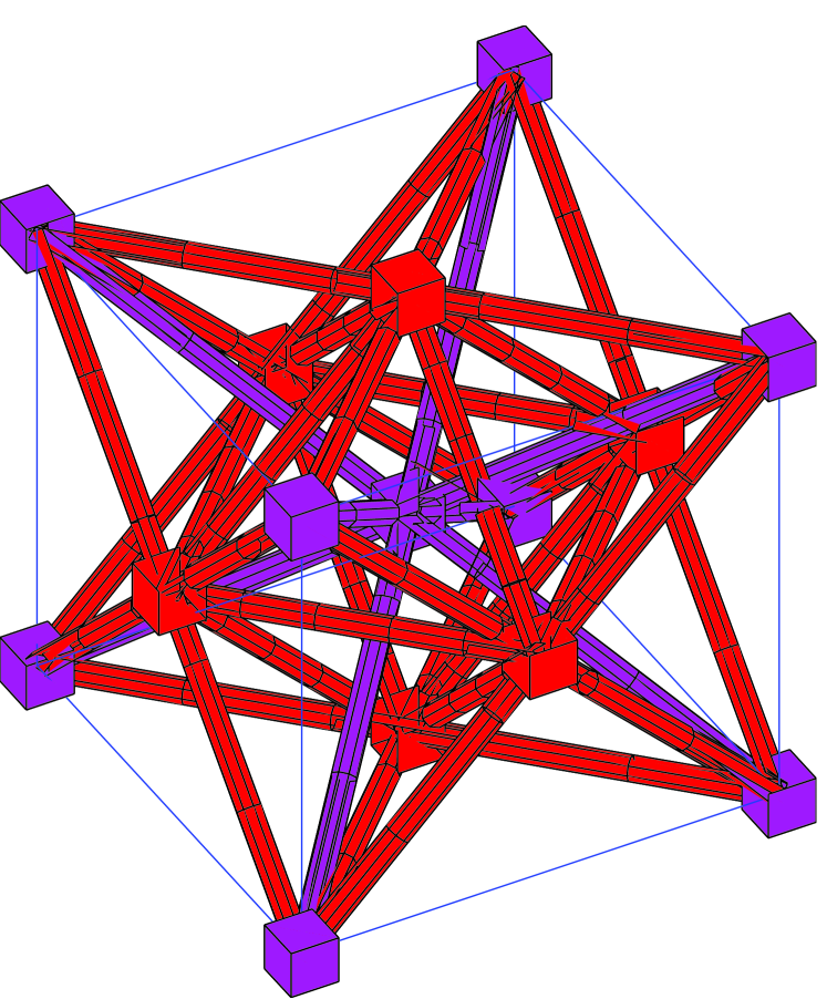
Figure 6: the red and magenta grids superimposed showing the nodes of the magenta grid at the corners and the centre of the (blue) cube. The nodes of the next coarser grid, magenta, are at the corners and centres of the cube as seen in Figure 6. Observe that the centre nodes of the magenta grid are not also nodes of the finer red grid; this causes some complications in the treatment of the two types of nodes. The magenta nodes at the corners are connected to twelve neighbours on the red grid so the natural average of the residuals is
(13) for corresponding to the magenta corner nodes. This average takes for each of nodes. The magenta nodes at the centre of the coarse (blue) cube is not connected to red nodes by the red grid, see Figure 6. However, it has six red nodes in close proximity, those at the centre of the faces, so the natural average is
(14) for corresponding to the magenta centre nodes. This averaging takes for each of nodes. The operation count for all of this restriction step from red to magenta is .
-
•
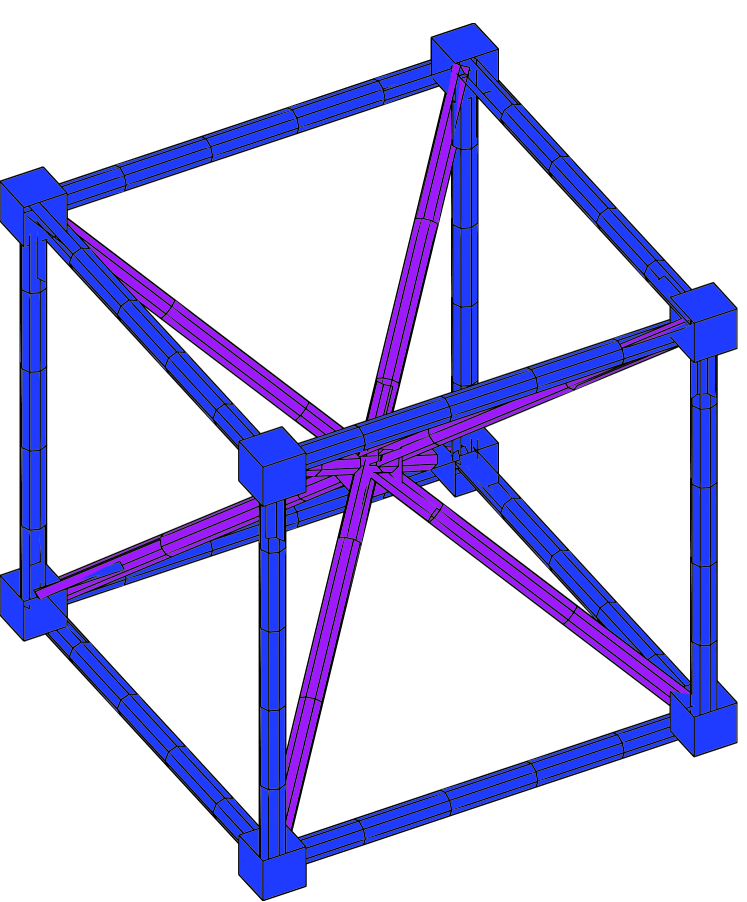
Figure 7: the magenta and blue grids superimposed showing the common nodes at the corners of the blue grid and the connections to the magenta centre node. The nodes of the coarse blue grid are at the corners of the shown cube, see Figure 7. On the magenta grid they are connected to eight neighbours, one for each octant, so the natural average of residuals from the magenta to the blue grid is
(15) for corresponding to the blue corner nodes. This averaging takes for each of blue nodes which thus totals .
These three restriction steps, to go up three levels of grids, thus total approximately . Hence, the entire restriction process, averaging the residuals, from a finest grid of spacing up levels to the coarsest grid of spacing takes
| (16) |
The simplest standard one-step restriction direct from the fine green grid to the blue grid takes approximately . Over the whole hierarchy this totals which is roughly half that of the proposed method. We anticipate that rapid convergence of the V-cycle makes the increase worthwhile.
3.2 The Jacobi prolongation steps
As in 2D, with this rich structure of grids we have no need to interpolate when prolongating from a coarse grid onto a finer grid; an appropriate “red-black” Jacobi iteration of the residual equation (2) avoids interpolation. Given an estimate of corrections at some blue level grid we proceed to the finer green grid via the following three prolongation steps.
-
•
Perform a magenta-blue Jacobi iteration on the nodes of the magenta grid shown in Figure 7. See that each node on the magenta grid is connected to eight neighbours distributed symmetrically about it, each contributes to an estimate of the Laplacian at the node. Thus, given initial approximations on the blue nodes from the coarser blue grid,
(17) for on the centre magenta nodes. The following blue-Jacobi iteration uses these updated values in the similar formula
(18) for on the corner blue nodes. In these formulae the over relaxation parameter has been introduced for later fine tuning; initially take . The operation count for this magenta-blue Jacobi iteration is on each of nodes giving a total of .
-
•
Perform a red-magenta Jacobi iteration on the nodes of the red grid shown in Figure 6. However, because the centre node (magenta) is not on the red grid, two features follow: it is not updated in this prolongation step; and it introduces a little asymmetry into the weights used for values at the nodes. The red nodes in the middle of each face are surrounded by four magenta nodes at the corners and two magenta nodes at the centres of the cube. However, the nodes at the centres are closer and so have twice the weight in the estimate of the Laplacian. Hence, given initial approximations on the magenta nodes from the coarser grid,
(19) for corresponding to the red nodes on the centre of faces normal to the -direction. Similar formulae apply for red nodes on other faces, cyclically permute the role of the indices. The over relaxation parameters and are introduced for later fine tuning; initially take . The following magenta-Jacobi iteration uses these updated values. Each magenta corner node in Figure 6 is connected to twelve red nodes and so is updated according to
(20) for all corresponding to corner magenta nodes. The operation count for this red-magenta Jacobi iteration is on each of nodes and on each of nodes. These total .
-
•
Perform a green-red Jacobi iteration on the nodes of the fine green grid shown in Figure 5. The green grid is a standard rectangular grid so the Jacobi iteration is also standard. Given initial approximations on the red nodes from the coarser red grid,
(21) for corresponding to the green nodes (edges and centre of the cube). The over relaxation parameter , initially , is introduced for later fine tuning. The red-Jacobi iteration uses these updated values in the similar formula
(22) for the red nodes in Figure 5. This prolongation step is a standard Jacobi iteration and takes on each of nodes for a total of .
These three prolongation steps together thus total . To prolongate over levels from the coarsest grid of spacing to the finest grid thus takes
| (23) |
The simplest trilinear interpolation direct from the blue grid to the green grid would take approximately , to be followed by for a Jacobi iteration on the fine green grid. Over the whole hierarchy this standard prolongation takes approximately . This total is smaller, but the proposed diagonal grid achieves virtually three Jacobi iterations instead of one and so is more effective.
3.3 The V-cycle converges well
Numerical experiments show that, as in 2D, although the operation count of the proposed algorithm is a little higher, the speed of convergence is much better. Both algorithms use to compute second-order accurate residuals on the finest grid. Thus the proposed method takes approximately for one V-cycle, some 37% more than the of the simplest standard algorithm. It achieves a mean factor of convergence . This rapid rate of convergence easily compensates for the small increase in computations taking half the number of flops per decimal digit accuracy determined.
| algorithm | per iter | per dig | |
|---|---|---|---|
| diagonal, | 0.140 | ||
| usual, | 0.477 | ||
| diagonal, | 0.659 | ||
| usual, | 0.651 |
As in 2D, fourth-order accurate solvers may be obtained simply by using the above second-order accurate V-cycle on the fourth-order accurate residuals evaluated on the finest grid. A compact fourth-order accurate scheme for the residuals is the 19 point formula
| (24) | |||||
Then using the V-cycle described above to determine corrections to the field leads to an increase in the operation count of solely from the extra computation in finding the finest residuals. Numerical experiments show that the multigrid iteration still converge, albeit slower, with . Table 2 shows that the rate of convergence on the diagonal hierarchy of grids is little different than that for the simplest usual multigrid algorithm. As in 2D, high accuracy, 4th order solutions to Poisson’s equation are best found by employing a first stage that finds 2nd order accurate solutions which are then refined in a second stage.
3.4 Optimise parameters of the V-cycle
As in 2D, the multigrid algorithms are improved by introducing some relaxation in the Jacobi iterations. The four parameters , , and were introduced in the Jacobi iterations (17–22) to do this, values bigger than 1 correspond to some over relaxation.
| algorithm | per iter | per dig | |||||
|---|---|---|---|---|---|---|---|
| diag, | 1.11 | 1.42 | 1.08 | 0.99 | 0.043 | ||
| usual, | 1.30 | 0.31 | |||||
| diag, | 0.91 | 0.80 | 0.70 | 1.77 | 0.39 | ||
| usual, | 1.70 | 0.41 |
The search for the optimum parameter set used the Nelder-Mead simplex method encoded in the procedure fmins in matlab. Searches were started from optimum parameters found for coarser grids. As tabulated in Table 3 the optimum parameters on a grid222Systematic searches on a finer grid were infeasible within one days computer time due to the large number of unknowns: approximately 30,000 components occur in the eigenvectors on a grid. were , , and and achieve an astonishingly fast rate of convergence of . This ensures convergence to a specified precision at half the cost of the similarly optimised, simple conventional multigrid algorithm.
For the fourth-order accurate residuals an optimised diagonal multigrid performs similarly to the optimised conventional multigrid with a rate of convergence of . Again fourth order accuracy is best obtained after an initial stage in which second order accuracy is used.
4 Conclusion
The use of a hierarchy of grids at angles to each other can halve the cost of solving Poisson’s equation to second order accuracy in grid spacing. Each iteration of the optimised simplest multigrid algorithm decreases errors by a factor of at least 20. This is true in both two and three dimensional problems. Further research is needed to investigate the effective of extra Jacobi iterations at each level of the diagonal grid.
When compared with the amazingly rapid convergence obtained for the second order scheme, the rate of convergence when using the fourth order residuals is relatively pedestrian. This suggests that a multigrid V-cycle specifically tailored on these diagonal grids for the fourth order accurate problem may improve convergence markedly.
There is more scope for W-cycles to be effective using these diagonal grids because there are many more levels in the multigrid hierarchy. An exploration of this aspect of the algorithm is also left for further research.
Acknowledgement:
This research has been supported by a grant from the Australian Research Council.
References
- [1] J.E. Dendy. Semicoarsening multgrid for systems. Elect. Trans. Num. Anal., 6:97–105, 1997.
- [2] M.M. Gupta, J. Kouatchou, and J. Zhang. Comparison of second- and fourth-order discretizations for multigrid Poisson solvers. J. Comput. Phys., 132:226–232, 1997.
- [3] S.O. Ibraheem and A.O. Demuren. On bi-grid local mode analysis of solution techniques for 3-D Euler and Navier-Stokes equations. J. Comput. Physics, 125:354—377, 1996.
- [4] R.K. Iyengar and A. Goyal. A note on multigrid for the three-dimensional Poisson equation in cylindrical coordinates. J. Comput. & Appl. Math., 33:163–169, 1990.
- [5] D.J. Mavriplis. Directional coarsening and smoothing for anisotropic Navier-Stokes problems. Elect. Trans. Num. Anal., 6:182–197, 1997.
- [6] D.J. Mavriplis. Unstructured grid techniques. Annu. Rev. Fluid Mech., 29:473–514, 1997.
- [7] J.D. Moulton, J.E. Dendy, and J.M. Hyman. The black box multigrid numerical homogenization algorithm. J. Comput. Physics, 142:80—108, 1998.
- [8] S.G. Sheffer, L. Martinelli, and A. Jameson. An efficient multigrid algorithm for compressible reactive flows. J. Comput. Physics, 144:484—516, 1998.
- [9] Jun Zhang. Fast and high accuracy multigrid solution of the three-dimensional Poisson equation. J. Comput. Phys., 143:449–461, 1998.