Reidemeister Torsion of 3-Dimensional
Euler Structures with Simple Boundary Tangency
and Legendrian Knots

Abstract. We generalize Turaev’s definition of torsion invariants of pairs $(M,\xi)$, where $M$ is a 3-dimensional manifold and $\xi$ is an Euler structure on $M$ (a non-singular vector field up to homotopy relative to $\partial M$ and local modifications in ${\rm Int}(M)$). Namely, we allow $M$ to have arbitrary boundary and $\xi$ to have simple (convex and/or concave) tangency circles to the boundary. We prove that Turaev’s $H_{1}(M)$-equivariance formula holds also in our generalized context. Our torsions apply in particular to (the exterior of) Legendrian links (in particular, knots) in contact 3-manifolds, and we prove that they can distinguish knots which are isotopic as framed knots but not as Legendrian knots. Using the combinatorial encoding of vector fields based on branched standard spines we show how to explicitly invert Turaev’s reconstruction map from combinatorial to smooth Euler structures, thus making the computation of torsions a more effective one. As an example we work out a specific computation.

Mathematics Subject Classification (1991): 57N10 (primary), 57Q10, 57R25 (secondary).

Introduction

Reidemeister torsion is a classical yet very vital topic in 3-dimensional topology, and it was recently used in a variety of important developments. To mention a few, torsion is a fundamental ingredient of the Casson-Walker-Lescop invariants (see e.g. [15]), and more generally of the perturbative approach to quantum invariants (see e.g. [14]). Relations have been pointed out between torsion and hyperbolic geometry [24]. Turaev’s torsion of Euler structures [27] has recently been recognized by Turaev himself ([28], [29]) to have deep connections with the Seiberg-Witten invariants of ${\rm Spin}^{\rm c}$-structures on 3-manifolds, after the proof of Meng and Taubes [20] that a suitable combination of these invariants can be identified with the classical Milnor torsion.

Turaev’s theory [27] actually exists in all dimensions. We quickly review it before proceeding. A smooth Euler structure $\xi$ on a compact oriented manifold $M$, possibly with $\partial M=\emptyset$, is a non-singular vector field on $M$ viewed up to local modifications in ${\rm Int}(M)$ and homotopy relative to $\partial M$. Turaev allows only “monochromatic” boundary components, i.e. black ones (on which the field points outwards) and white ones (on which it points inwards). This implies the constraint that $\chi(M,W)=0$, where $W$ is the white portion of $\partial M$, but in [28] and [29] Turaev only focuses on the more specialized case where $M$ is 3-dimensional and closed or bounded by tori. In all dimensions, the set ${\rm Eul}^{\rm s}(M,W)$ of smooth Euler structures compatible with $(M,W)$ is an affine space over $H_{1}(M;{\hbox{\Bbb Z}})$. The two main ingredients of Turaev’s theory are as follows. First, he defines a certain set of $1$-chains, called the space ${\rm Eul}^{\rm c}(M,W)$ of combinatorial Euler structures compatible with $(M,W)$, he shows that this is again affine over $H_{1}(M;{\hbox{\Bbb Z}})$, and he describes an $H_{1}(M;{\hbox{\Bbb Z}})$-equivariant bijection $\Psi:{\rm Eul}^{\rm c}(M,W)\to{\rm Eul}^{\rm s}(M,W)$ called the reconstruction map. Second, for $\xi\in{\rm Eul}^{\rm c}(M,W)$ and for any representation $\varphi$ of $\pi_{1}(M)$ into the units of a suitable ring $\Lambda$ he defines a torsion invariant $\tau^{\varphi}(M,\xi)$, or more generally $\tau^{\varphi}(M,\xi,{\hbox{\Got h}})$, with values in $K_{1}(\Lambda)/(\pm 1)$. This invariant is by definition a lifting of the classical Reidemeister torsion (see [21]) $\tau^{\varphi}(M)\in K_{1}(\Lambda)/(\pm\varphi(\pi_{1}(M)))$, and it satisfies the $H_{1}(M;{\hbox{\Bbb Z}})$-equivariance formula

$$\tau^{\varphi}(M,\xi^{\prime},{\hbox{\Got h}})=\tau^{\varphi}(M,\xi,{\hbox{\Got h}})\cdot\varphi(\xi^{\prime}-\xi)$$ (1)

where $\xi^{\prime}-\xi\in H_{1}(M;{\hbox{\Bbb Z}})$. For $\xi\in{\rm Eul}^{\rm s}(M,W)$ one defines $\tau^{\varphi}(M,\xi)$ as $\tau^{\varphi}(M,\Psi^{-1}(\xi))$, and the $H_{1}(M;{\hbox{\Bbb Z}})$-equivariance of the reconstruction map $\Psi$ implies that formula (1) holds also for smooth structures. We emphasize that the definition of $\Psi$ is based on an explicit geometric construction, but its bijectivity is only established through $H_{1}(M;{\hbox{\Bbb Z}})$-equivariance. This makes the definition of torsion for smooth structures somewhat implicit.

In the present paper, and in other papers in preparation, we are concerned with generalizations and improvements of Turaev’s theory. Here we consider 3-manifolds. This work had two main initial aims. Our first aim was to find a geometric description of the map $\Psi^{-1}$, and hence to turn the computation of Turaev’s torsion into a more effective procedure, using our combinatorial encoding [2] of non-singular vector fields up to homotopy (also called “combings”) in terms of branched standard spines. Our second aim was to define torsion invariants of (pseudo-)Legendrian links, i.e. links tangent to a given plane field, viewed up to tangency-preserving isotopy (when the plane field is a contact structure one gets the familiar notion of Legendrian link and Legendrian isotopy). A specific motivation to look for invariants of pseudo-Legendrian links comes from the remarkable relation recently discovered by Fintushel and Stern [10] between the Alexander polynomial (i.e. Milnor torsion) of a knot $K\subset S^{3}$ and (a suitable combination of) the Seiberg-Witten invariants of the “surgered” $4$-manifold $X_{K}$ obtained using $K$ (and a suitable base $4$-manifold $X$). Both our initial aims lead us to consider Euler structures on $3$-manifolds $M$ (without restrictions on $\partial M$) allowing simple tangency circles to $\partial M$ of concave type (see Fig. 1 below). On the other hand it turns out that, to define torsions, the natural objects to deal with are Euler structures with convex tangency circles. It is a fortunate fact, peculiar of dimension 3, that there is a canonical way to associate a convex field to any simple (i.e. mixed concave and convex) one. This allows to define torsion for all smooth simple Euler structures, and eventually to achieve both the objectives we had in mind.

Let us now summarize the contents of this paper. The foundational part of our work consists in extending to the context of Euler structures with simple tangency the notions of combinatorial structure ${\rm Eul}^{\rm c}$ and reconstruction map $\Psi$. This part follows the same scheme as [27] and relies on technical results of Turaev. Our main contribution here is the proof that the natural transformations of a concave structure into a convex one, viewed at the smooth level and at the combinatorial level, actually correspond to each other under the reconstruction map (Theorem 1.9). After setting the foundations, we prove the following main results (stated informally here: see Sections 1 and 2 for precise definitions and statements.)

Theorem 0.1

There exist pairs $(M,\eta)$, where $\eta$ is an oriented plane distribution on $M$, and knots $K_{0}$, $K_{1}$ tangent to $\eta$ (whence framed), such that:

1. $K_{0}$ and $K_{1}$ are isotopic as framed knots;

2. A torsion invariant shows that $K_{0}$ and $K_{1}$ are not isotopic to each other through knots tangent to $\eta$.

Moreover, $\eta$ can be chosen to be a contact structure.

Theorem 0.2

Let $\xi$ be an Euler structure with concave tangency circles. If $P$ is a branched standard spine which represents $\xi$, then $P$ allows to explicitly find a representative of $\Psi^{-1}(\xi)\in{\rm Eul}^{\rm c}$, and hence to compute the torsion of $\xi$ in terms of the finite combinatorial data which encode $P$.

Concerning Theorem 0.1, the relation with vector fields is of course given by taking the orthogonal to $\eta$. Note that our torsions are defined not only for knots but also for links, including homologically non-trivial Legendrian links, for which the usual invariants, such as the rotation number (Maslov index), are not defined. However we will show that, in a suitable sense, torsion is a generalization of the rotation number, when the latter is defined. Moreover we will prove that torsions are sensitive to an analogue of the winding number.

Another relevant point concerning Theorem 0.1 is that in general torsion does not provide a single-valued invariant for pseudo-Legendrian knots, because the action of a certain mapping class group must be taken into account. However we will show that for many knots this action is actually trivial, so torsion is indeed single-valued. This is the case for instance for all knots contained in homology spheres. So our torsion invariants include a (non-trivial) refinement of the Alexander polynomial to Legendrian knots in $S^{3}$.

This paper is organized as follows. In Section 1 we provide the formal definitions of smooth and combinatorial Euler structures, we informally introduce torsion and we state the fundamental results which imply that torsion is well-defined and $H_{1}$-equivariant. In Section 2 we specialize to knot exteriors and we prove that torsion is a non-trivial invariant of Legendrian knots, as announced above. In Section 3 we address the main technical points of the definition of torsion. In Section 4 we show how branched standard spines can be used for computing torsion, and in Section 5 we actually carry out a computation. In Sections 1 to 4 proofs which are long and require the introduction of ideas and techniques not used elsewhere are omitted. Section 6 contains all these proofs.

We conclude this introduction by announcing related results which we have recently obtained and currently writing down. In [4] we extend to the case with boundary our combinatorial presentation [2] of combed manifolds in terms of branched spines (this extension is actually mentioned also in the present paper —see Section 4). Using this presentation we develop an approach to torsion entirely based on combinatorial techniques (branched spines), leading to a generalization of Turaev’s theory slightly different from the present paper’s. In [5] we generalize the theory of Euler structures and (with some restrictions) of torsions to all dimensions and allowing any generic (Whitney-Morin-type) tangency to the boundary. Noting that this situation arises when one cuts a manifold along a hypersurface in general position with respect to a given non-singular vector field, one is naturally lead to the question of how Euler structures and torsion behave under glueing. As a motivation, note that a similar question is involved in the summation formulae for the Casson invariant (see [16]), and is faced also in [10], [20] and [29]. We believe that this question deserves further investigation.

1 Main definitions and statements

In this section we define Euler structures and their torsion. Fix once and for ever a compact oriented 3-manifold $M$, possibly with $\partial M=\emptyset$. Using the Hauptvermutung, we will always freely intermingle the differentiable, piecewise linear and topological viewpoints. Homeomorphisms will always respect orientations. All vector fields mentioned in this paper will be non-singular, and they will be termed just fields for the sake of brevity.

Smooth and combinatorial Euler structures.

We will call boundary pattern on $M$ a partition ${\cal P}=(W,B,V,C)$ of $\partial M$ where $V$ and $C$ are finite unions of disjoint circles, and $\partial W=\partial B=V\cup C$. In particular, $W$ and $B$ are interiors of compact surfaces embedded in $\partial M$. Even if ${\cal P}$ can actually be determined by less data, e.g. the pair $(W,V)$, we will find it convenient to refer to ${\cal P}$ as a quadruple. Points of $W$, $B$, $V$ and $C$ will be called white, black, convex and concave respectively. We define the set of smooth Euler structures on $M$ compatible with ${\cal P}$, denoted by ${\rm Eul}^{\rm s}(M,{\cal P})$, as the set of equivalence classes of fields on $M$ which point inside on $W$, point outside on $B$ and have simple tangency to $\partial M$ of convex type along $V$ and concave type along $C$, as shown in a cross-section in Fig. 1.

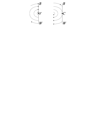
Figure 1: Convex (left) and concave (right) tangency to the boundary.

Two such fields are equivalent if they are obtained from each other by homotopy through fields of the same type and modifications supported into interior balls. The following variation on the Poincaré-Hopf formula is established in Section 6:

Proposition 1.1

${\rm Eul}^{\rm s}(M,{\cal P})$ is non-empty if and only if $\chi({\overline{W}})=\chi(M)$.

We remark here that $\chi({\overline{W}})=\chi(W)$, $\chi(\overline{B})=\chi(B)$, $\chi(V)=\chi(C)=0$ and $\chi(W)+\chi(B)=\chi(\partial M)=2\chi(M)$, so there are various ways to rewrite the relation $\chi({\overline{W}})=\chi(M)$, the most intrinsic of which is actually $\chi(M)-(\chi({\overline{W}})-\chi(C))=0$ (see below for the reason).

Now, given $\xi,\xi^{\prime}\in{\rm Eul}^{\rm s}(M,{\cal P})$ we can choose generic representatives $v,v^{\prime}$, so that the set of points of $M$ where $v^{\prime}=-v$ is a union of loops contained in the interior of $M$. A standard procedure allows to give these loops a canonical orientation, thus getting an element $\alpha^{\rm s}(\xi,\xi^{\prime})\in H_{1}(M;{\hbox{\Bbb Z}})$. The following result is easily obtained along the lines of the well-known analogue for closed manifolds.

Lemma 1.2

$\alpha^{\rm s}$ is well-defined and turns ${\rm Eul}^{\rm s}(M,{\cal P})$ into an affine space over $H_{1}(M;{\hbox{\Bbb Z}})$.

A (finite) cellularization ${\cal C}$ of $M$ is called suited to ${\cal P}$ if $V\cup C$ is a subcomplex, so $W$ and $B$ are unions of cells. Here and in the sequel by “cell” we will always mean an open one. Let such a ${\cal C}$ be given. For $\sigma\in{\cal C}$ define ${\rm ind}(\sigma)=(-1)^{{\rm dim}(\sigma)}$. We define ${\rm Eul}^{\rm c}(M,{\cal P})_{\cal C}$ as the set of equivalence classes of integer singular 1-chains $z$ in $M$ such that

$$\partial z=\sum_{\sigma\subset M\setminus(W\cup V)}{\rm ind}(\sigma)\cdot p_{\sigma}$$

where $p_{\sigma}\in\sigma$ for all $\sigma$. Two chains $z$ and $z^{\prime}$ with $\partial z=\sum{\rm ind}(\sigma)\cdot p_{\sigma}$ and $\partial z^{\prime}=\sum{\rm ind}(\sigma)\cdot p^{\prime}_{\sigma}$ are defined to be equivalent if there exist $\delta_{\sigma}:([0,1],0,1)\to(\sigma,p_{\sigma},p^{\prime}_{\sigma})$ such that

$$z-z^{\prime}+\sum_{\sigma\subset M\setminus(W\cup V)}{\rm ind}(\sigma)\cdot\delta_{\sigma}$$

represents $0$ in $H_{1}(M;{\hbox{\Bbb Z}})$. Elements of ${\rm Eul}^{\rm c}(M,{\cal P})_{\cal C}$ are called combinatorial Euler structures relative to ${\cal P}$ and ${\cal C}$, and their representatives are called Euler chains. The definition implies that, for $\xi,\xi^{\prime}\in{\rm Eul}^{\rm c}(M,{\cal P})_{\cal C}$, their difference $\xi-\xi^{\prime}$ can be defined as an element $\alpha^{\rm c}(\xi,\xi^{\prime})$ of $H_{1}(M;{\hbox{\Bbb Z}})$. The following is easy:

Lemma 1.3

${\rm Eul}^{\rm c}(M,{\cal P})_{\cal C}$ is non-empty if and only if $\chi({\overline{W}})=\chi(M)$, and in this case $\alpha^{\rm c}$ turns it into an affine space over $H_{1}(M;{\hbox{\Bbb Z}})$.

Since ${\overline{W}}=W\cup V\cup C$, the alternating sum of dimensions of cells in $W\cup V$ is intrinsically interpreted as $\chi({\overline{W}})-\chi(C)$, which explains why the most meaningful way to write the relation $\chi({\overline{W}})=\chi(M)$ is $\chi(M)-(\chi({\overline{W}})-\chi(C))=0$. From now on we will always assume that this relation holds. Turaev [27] only considers the case where $V=C=\emptyset$, so $W=\overline{W}$ and $B=\overline{B}$, and our relation takes the usual form $\chi(M,W)=0$. The following result was established by Turaev in [27] in his setting, but the proof extends verbatim to our context, so we omit it. Only the first assertion is hard. We state the other two because we will use them.

Proposition 1.4

1. If ${\cal C}^{\prime}$ is a subdivision of ${\cal C}$ then there exists a canonical $H_{1}(M;{\hbox{\Bbb Z}})$-isomorphism ${\rm Eul}^{\rm c}(M,{\cal P})_{\cal C}\to{\rm Eul}^{\rm c}(M,{\cal P})_{{\cal C}^{\prime}}$. In particular ${\rm Eul}^{\rm c}(M;{\hbox{\Bbb Z}})$ is canonically defined up to $H_{1}(M;{\hbox{\Bbb Z}})$-isomorphism independently of the cellularization.

2. If ${\cal C}$ is a cellularization of $M$ suited to ${\cal P}$ and $x_{0}\in M$ is an assigned point, any element of ${\rm Eul}^{\rm c}(M,{\cal P})$ can be represented, with respect to ${\cal C}$, as a sum $\sum_{\sigma\subset M\setminus(W\cup V)}{\rm ind}(\sigma)\cdot\beta_{\sigma}$ with $\beta_{\sigma}:([0,1],0,1)\to(M,x_{0},\sigma)$.

3. If ${\cal T}$ is a triangulation of $M$ suited to ${\cal P}$, any element of ${\rm Eul}^{\rm c}(M,{\cal P})$ can be represented, with respect to ${\cal T}$, as a simplicial $1$-chain in the first barycentric subdivision of ${\cal T}$.

Our first main result, proved in Section 6, is the extension to the case under consideration of Turaev’s correspondence between ${\rm Eul}^{\rm c}$ and ${\rm Eul}^{\rm s}$.

Theorem 1.5

There exists a canonical $H_{1}(M;{\hbox{\Bbb Z}})$-equivariant isomorphism

$$\Psi:{\rm Eul}^{\rm c}(M,{\cal P})\to{\rm Eul}^{\rm s}(M,{\cal P}).$$

The definition of $\Psi$ is based on an explicit geometric construction, but its bijectivity is only established through $H_{1}(M;{\hbox{\Bbb Z}})$-equivariance. As already mentioned in the introduction, this makes in general a very difficult task to determine the inverse of $\Psi$. One of the features of this paper is the description of $\Psi^{-1}$ in terms of the combinatorial encoding of fields by means of branched spines: Theorem 4.9 describes $\Psi^{-1}$ when ${\cal P}$ is concave, and Theorem 1.9 shows that from a general ${\cal P}$ we can effectively pass to a unique convex ${\cal P}$, and hence to a unique concave ${\cal P}$, and conversely.

In view of Theorem 1.5, when no confusion risks to arise, we shortly write ${\rm Eul}(M,{\cal P})$ for either ${\rm Eul}^{\rm s}(M,{\cal P})$ or ${\rm Eul}^{\rm c}(M,{\cal P})$, and $\alpha$ for the map giving the affine $H_{1}(M;{\hbox{\Bbb Z}})$-structure on this space. Before turning to torsions, as announced in the introduction, we show that (pseudo-)Legendrian links naturally define Euler structures of the type we are considering.

Remark 1.6

Assume $M$ is closed, let $v$ be a field on $M$ and let $L$ be a link in $M$ transverse to $v$. If we take a small enough regular neighbourhood $U(L)$ of $L$, the field $v$ will be tangent to $\partial U(L)$ only along two lines on each component, and the tangency, viewed from the exterior $E(L)=M\setminus U(L)$, has concave type (see the cross-section in Fig. 2).

Figure 2: Concave tangency on a link exterior.

This shows that the triple $(M,v,L)$ defines an element of $\xi(M,v,L)$ of ${\rm Eul}^{\rm s}(E(L),{\cal P})$, where ${\cal P}=(W,B,\emptyset,C)$ depends on the framing induced by $v$ on $L$. Note that if $\eta$ is a cooriented plane distribution and $L$ is tangent to $\eta$ then the definition $\xi(M,\eta^{\perp},L)$ applies. When $\eta$ is a contact structure $L$ is called a Legendrian link, so we will call it pseudo-Legendrian in general. In Section 2 we shall see that $\xi(M,\eta^{\perp},L)$ can be used to construct non-trivial invariants for pseudo-Legendrian isotopy classes of knots.

Convex Euler structure associated to an arbitrary one.

Let $M$ and ${\cal P}=(W,B,V,C)$ be as in the definition of ${\rm Eul}(M,{\cal P})$. The pattern $\theta({\cal P})=(W,B,V\cup C,\emptyset)$ is a convex one canonically associated to ${\cal P}$. We define a map

$$\Theta^{\rm s}:{\rm Eul}^{\rm s}(M,{\cal P})\to{\rm Eul}^{\rm s}(M,\theta({\cal P}))$$

as geometrically described in Fig. 3. Concerning this figure, note that the loops in $C$ can be oriented as components of the boundary of $B$, which is oriented as a subset of the boundary of $M$.

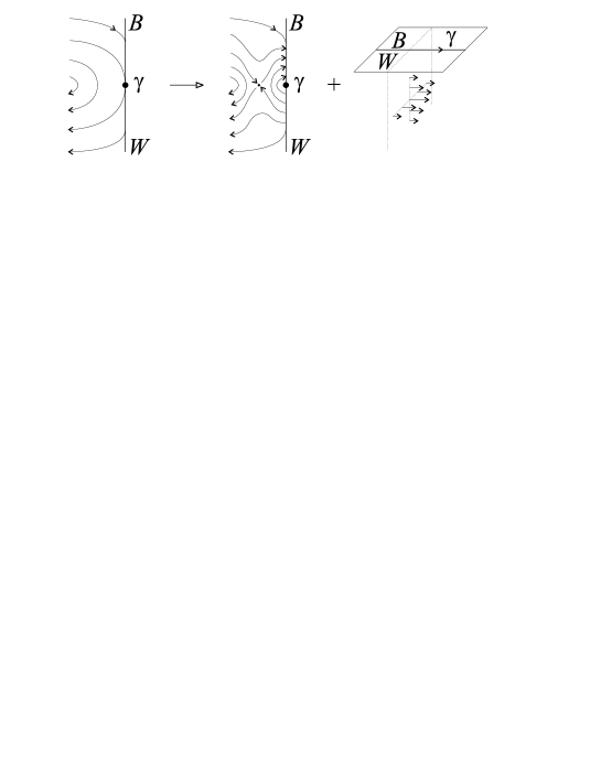
Figure 3: Turning a concave tangency circle $\gamma$ into a convex one: the apparent singularity in the cross-section is removed by adding a small bell-shaped field directed parallel to $\gamma$, i.e. orthogonal to the cross-section.

Lemma 1.7

$\Theta^{\rm s}$ is a well-defined $H_{1}(M;{\hbox{\Bbb Z}})$-equivariant bijection.

Proof of  1.7. The first two properties are easy and imply the third property. The inverse of $\Theta^{\rm s}$ may actually be described geometrically by a figure similar to Fig. 3, but we leave this to the reader.  1.7

We define now a combinatorial version of $\Theta^{\rm s}$. Consider a cellularization ${\cal C}$ suited to ${\cal P}$, and denote by $\gamma_{1},\dots,\gamma_{n}$ the 1-cells contained in $C$. We choose the parameterizations $\gamma_{j}:(0,1)\to C$ so that they respect the natural orientation of $C$ already discussed above, and we extend the $\gamma_{j}$ to $[0,1]$, without changing notation. Now let $z$ be an Euler chain relative to ${\cal P}$. It easily seen that $z-\sum_{j=1}^{n}\gamma_{j}\big{|}_{[1/2,1]}$ is an Euler chain relative to $\theta({\cal P})$. Setting

$$\Theta^{\rm c}([z])=\left[z-\sum_{j=1}^{n}\gamma_{j}\big{|}_{[1/2,1]}\right]$$

we get a map $\Theta^{\rm c}:{\rm Eul}^{\rm c}(M,{\cal P})\to{\rm Eul}^{\rm c}(M,\theta({\cal P}))$.

Lemma 1.8

$\Theta^{\rm c}$ is a well-defined $H_{1}(M;{\hbox{\Bbb Z}})$-equivariant bijection.

Proof of  1.8. Again, the first two properties are easy and imply the third one.  1.8

In Section 6 we will see the following:

Theorem 1.9

If $\Psi$ is the reconstruction map of Theorem 1.5 then the following diagram is commutative:

$$\matrix{{\rm Eul}^{\rm c}(M,{\cal P})&\stackrel{{\scriptstyle\Theta^{\rm c}}}{{\longrightarrow}}&{\rm Eul}^{\rm c}(M,\theta({\cal P}))\phantom{.}\cr\Psi\downarrow\phantom{\Psi}&&\phantom{\Psi}\downarrow\Psi\cr{\rm Eul}^{\rm s}(M,{\cal P})&\stackrel{{\scriptstyle\Theta^{\rm s}}}{{\longrightarrow}}&{\rm Eul}^{\rm s}(M,\theta({\cal P})).\cr}$$

Using this result we will sometimes just write $\Theta:{\rm Eul}(M,{\cal P})\to{\rm Eul}(M,\theta({\cal P}))$.

Torsion of a (convex) Euler structure.

Let us first briefly review the algebraic setting [21] in which torsions can be defined. We consider a ring $\Lambda$ with unit, with the property that if $n$ and $m$ are distinct positive integers then $\Lambda^{n}$ and $\Lambda^{m}$ are not isomorphic as $\Lambda$-modules. The Whitehead group $K_{1}(\Lambda)$ is defined as the Abelianization of ${\rm GL}_{\infty}(\Lambda)$, and ${\overline{K}}_{1}(\Lambda)$ is the quotient of $K_{1}(\Lambda)$ under the action of $-1\in{\rm GL}_{1}(\Lambda)=\Lambda_{*}$. Now consider a convex boundary pattern ${\cal P}=(W,B,V,\emptyset)$ on a manifold $M$, take a representation $\varphi:\pi_{1}(M)\to\Lambda_{*}$, and consider the $\Lambda$-modules $H^{\varphi}_{i}(M,W\cup V)$ of relative twisted homology (see Section 3 for a reminder on the definition). Notice that $W\cup V={\overline{W}}$, so if we have a cellularization of $M$ suited to ${\cal P}$ then $W\cup V$ is a (closed) subcomplex, and we can use the cellular theory to compute $H^{\varphi}_{i}(M,W\cup V)$. This is the reason for considering convex boundary patterns.

Assume now that $H^{\varphi}_{i}(M,W\cup V)$ is free, and choose a $\Lambda$-basis ${\hbox{\Got h}}_{i}$. Then a torsion $\tau^{\varphi}(M,W\cup V,{\hbox{\Got h}})\in{\overline{K}}_{1}(\Lambda)/\varphi(\pi_{1}(M))$ can be defined as in [21]. Here the action of $\varphi(\pi_{1}(M))$ has to be taken into account because of the ambiguity of the choice of liftings to the universal cover of the cells of $M\setminus(W\cup V)$. It was an intuition of Turaev [27], which we extend in this paper to include the case of simple tangency, that an Euler structure $\xi\in{\rm Eul}(M,{\cal P})$ can be used to get rid of the action of $\varphi(\pi_{1}(M))$. More precisely we will show below the following:

Theorem 1.10

In the above situation a torsion $\tau^{\varphi}(M,{\cal P},\xi,{\hbox{\Got h}})$ can be defined. The reduction modulo $\varphi(\pi_{1}(M))$ of $\tau^{\varphi}(M,{\cal P},\xi,{\hbox{\Got h}})$ gives $\tau^{\varphi}(M,W\cup V,{\hbox{\Got h}})$. Moreover if $\xi,\xi^{\prime}\in{\rm Eul}(M,{\cal P})$ then

$$\tau^{\varphi}(M,{\cal P},\xi^{\prime},{\hbox{\Got h}})=\tau^{\varphi}(M,{\cal P},\xi,{\hbox{\Got h}})\cdot\overline{\varphi}(\alpha(\xi^{\prime},\xi)).$$ (2)

For a formal definition of $\overline{\varphi}:H_{1}(M;{\hbox{\Bbb Z}})\to{\overline{K}}_{1}(\Lambda)$ see Section 3. A self-contained definition of $\tau^{\varphi}(M,{\cal P},\xi,{\hbox{\Got h}})$ will also be given in Section 3. For the readers already acquainted with [21], we mention the key point: given a cellularization of $M$ suited to ${\cal P}$, a preferred family of liftings for the cells in $M\setminus(W\cup V)$ is found by representing $\xi$ by a “connected spider” as in point 2 of Proposition 1.4, lifting the spider starting from an arbitrary lifting of its head, and defining the preferred cell-liftings as those containing the ends of the legs of the lifted spider.

Theorem 1.10 only applies to convex patterns, but if ${\cal P}$ is not convex we can use the canonical map $\Theta:{\rm Eul}(M,{\cal P})\to{\rm Eul}(M,\theta({\cal P})$ and define

$$\tau^{\varphi}(M,{\cal P},\xi,{\hbox{\Got h}})=\tau^{\varphi}(M,\theta({\cal P}),\Theta(\xi),{\hbox{\Got h}}).$$

Of course the equivariance formula (2) still holds.

One of the important features of Theorem 1.10 is that if we start from a combinatorial representative of $\xi$ then the computation of $\tau^{\varphi}(M,{\cal P},\xi,{\hbox{\Got h}})$ is (in principle) algorithmic, provided we start from an explicit description of the universal cover of $M$ (or the maximal Abelian cover, which is often easier, when $\Lambda$ is commutative).

The next result follows directly from the definition but is nonetheless worth stating, because it shows how torsions may be used to distinguish triples $(M,{\cal P},\xi)$ from each other (see Section 2 for a relevant consequence).

Proposition 1.11

Let $f:M\to M^{\prime}$ be a homeomorphism, consider $\xi\in{\rm Eul}(M,{\cal P})$, $\varphi:\pi_{1}(M)\to\Lambda_{*}$ and a $\Lambda$-basis h of $H^{\varphi}_{*}(M,\overline{W})$. Then

$$\tau^{\varphi\circ f_{*}^{-1}}(M^{\prime},f_{*}({\cal P}),f_{*}(\xi),f_{*}({\hbox{\Got h}}))=\tau^{\varphi}(M,{\cal P},\xi,{\hbox{\Got h}}).$$

2 Torsion of pseudo-Legendrian knots

We fix in this section a compact oriented manifold $M$ and a boundary pattern ${\cal P}$ on $M$. The boundary of $M$ may be empty or not. Recall that if $v$ is a vector field on $M$ and $K$ is a knot in ${\rm Int}(M)$, we have defined $K$ to be pseudo-Legendrian in $(M,v)$ if $v$ is transversal to $K$. We will also call $(v,K)$ a pseudo-Legendrian pair. Having fixed ${\cal P}$, we will only consider fields $v$ compatible with ${\cal P}$. The aim of this section is to show how torsions can be applied to distinguish pseudo-Legendrian knots. Some of the results we will establish hold also for links, but we will stick to knots for the sake of simplicity. First, we need to spell out the equivalence relation which we consider.

Let $v_{0},v_{1}$ be compatible with ${\cal P}$ and let $K_{0},K_{1}$ be pseudo-Legendrian in $(M,v_{0})$ and $(M,v_{1})$ respectively. We define $(v_{0},K_{0})$ to be weakly equivalent to $(v_{1},K_{1})$ if there exist a homotopy $(v_{t})_{t\in[0,1]}$ through fields compatible with ${\cal P}$ and an isotopy $(K_{t})_{t\in[0,1]}$ such that $K_{t}$ is transversal to $v_{t}$ for all $t$. If $v_{0}=v_{1}$ then $K_{0}$ and $K_{1}$ are called strongly equivalent if the homotopy $(v_{t})$ can be chosen to be constant.

Remark 2.1

Of course strong equivalence implies weak equivalence. Weak equivalence is the natural relation to consider on pseudo-Legendrian pairs $(v,K)$, while strong equivalence is natural for pseudo-Legendrian knots in a fixed $(M,v)$. We will see that torsion provides obstructions to weak (and hence to strong) equivalence.

Now let $K$ be pseudo-Legendrian in $(M,v)$ and note that $v$ turns $K$ into a framed knot, which we will denote by $K^{(v)}$. The framed-isotopy class of $K^{(v)}$ is of course invariant under weak equivalence, so we will only try to distinguish knots which are framed-isotopic to each other. As already mentioned, the idea is to restrict $v$ to the exterior of $K$ and consider the induced Euler structure. A technical subtlety arises here, because the comparison class of two such Euler structures coming from framed-isotopic knots cannot be computed directly. It will turn out that the action of a group must be taken into account. However, we will see that for important classes of knots this action can actually be neglected.

Euler structures on knot exteriors.

For a knot $K$ in $M$ we consider a (closed) tubular neighbourhood $U(K)$ of $K$ in $M$ and we define $E(K)$ as the closure of the complement of $U(K)$. If $F$ is a framing on $K$ we extend the boundary pattern ${\cal P}$ previously fixed on $M$ to a boundary pattern ${\cal P}(K^{F})$ on $E(K)$, by splitting $\partial U(K)$ into a white and a black longitudinal annuli, the longitude being the one defined by the framing $F$. As a direct application of Proposition 1.1 one sees that ${\rm Eul}(E(K),{\cal P}(K^{F}))$ is non-empty (assuming ${\rm Eul}(M,{\cal P})$ to be non-empty).

A convenient way to think of ${\cal P}(K^{F})$ is as follows. The framing $F$ determines a transversal vector field along $K$. If we extend this field near $K$ and choose $U(K)$ small enough then the pattern we see on $\partial U(K)$ is exactly as required. With this picture in mind, it is clear that if $K$ is pseudo-Legendrian in $(M,v)$, where $v$ is compatible with ${\cal P}$, then the restriction of $v$ to $E(K)$ defines an element

$$\xi(v,K)\in{\rm Eul}(E(K),{\cal P}(K^{(v)}).$$

(This notation is consistent with that previously used, because in this section we are considering $M$ to be fixed.)

Group action on Euler structures.

Consider a knot $K$ and a self-diffeomorphism $f$ of $E(K)$ which is the identity near $\partial E(K)$. Then $f$ extends to a self-diffeomorphism $\widehat{f}$ of $M$, where $\widehat{f}\big{|}_{U(K)}={\rm id}_{U(K)}$. We define $G(K)$ as the group of all such $f$’s with the property that $\widehat{f}$ is isotopic to the identity on $M$. Elements of $G(K)$ are regarded up to isotopy relative to $\partial E(K)$. If $F$ is a framing on $K$ then the pull-forward of vector fields induces an action of $G(K)$ on ${\rm Eul}(E(K),{\cal P}(K^{(v)})$. We will now see that an obstruction to weak equivalence can be expressed in terms this group action.

Let $(v_{0},K_{0})$ and $(v_{1},K_{1})$ be pseudo-Legendrian pairs in $M$, and assume that $K_{0}^{(v_{0})}$ is framed-isotopic to $K_{1}^{(v_{1})}$ under a diffeomorphism $f$ relative to $\partial M$. Using the restriction of $f$ and the pull-back of vector fields we get a bijection

$$f^{*}:{\rm Eul}(E(K_{1}),{\cal P}(K_{1}^{(v_{1})}))\to{\rm Eul}(E(K_{0}),{\cal P}(K_{0}^{(v_{0})})).$$

Proposition 2.2

Under the current assumptions, if $(v_{0},K_{0})$ and $(v_{1},K_{1})$ are weakly equivalent to each other then $f^{*}(\xi(v_{1},K_{1}))$ belongs to the $G(K_{0})$-orbit of $\xi(v_{0},K_{0})$ in ${\rm Eul}(E(K_{0}),{\cal P}(K_{0}^{(v_{0})})$.

Proof of  2.2. By assumption $K_{0},K_{1}$ and $v_{0},v_{1}$ embed in continuous families $(K_{t})_{t\in[0,1]}$ and $(v_{t})_{t\in[0,1]}$, where $v_{t}$ is transversal to $K_{t}$ for all $t$. Now $(K_{t}^{(v_{t})})_{t\in[0,1]}$ is a framed-isotopy, so there exists a continuous family $(g_{t})_{t\in[0,1]}$ of diffeomorphisms of $M$ fixed on $\partial M$ and such that $g_{0}={\rm id}_{M}$ and $g_{t}(K_{0}^{(v_{0})})=K_{t}^{(v_{t})}$. So we get a map

$$[0,1]\ni t\mapsto\alpha(\xi(v_{0},K_{0}),g_{t}^{*}(\xi(v_{t},K_{t})))\in H_{1}(E(K_{0});{\hbox{\Bbb Z}}).$$

Since $H_{1}(E(K_{0});{\hbox{\Bbb Z}})$ is discrete and the map is continuous, we deduce that the map is identically 0. So $g_{1}^{*}(\xi(v_{1},K_{1}))=\xi(v_{0},K_{0})$. Now

$$f^{*}(\xi(v_{1},K_{1}))=(f^{*}\,{\scriptstyle\circ}\,(g_{1})_{*}\,{\scriptstyle\circ}\,g_{1}^{*})(\xi(v_{1},K_{1}))=(f^{-1}\,{\scriptstyle\circ}\,g_{1})_{*}(\xi(v_{0},K_{0}))$$

and the conclusion follows because $f^{-1}\,{\scriptstyle\circ}\,g_{1}$ defines an element of $G(K_{0})$.  2.2

The group $G(K)$ is in general rather difficult to understand (see [12]), so we introduce a special terminology for the case where its action can be neglected. We will say that a framed knot $K^{F}$ is good if $G(K)$ acts trivially on ${\rm Eul}(E(K),{\cal P}(K^{F}))$. If $K^{F}$ is good for all framings $F$, we will say that $K$ itself is good. The following are easy examples of good knots:

• $M$ is $S^{3}$ and $K$ is the trivial knot;

• $M$ is a lens space $L(p,q)$ and $K$ is the core of one of the handlebodies of a genus-one Heegaard splitting of $M$.

The reason is that in both cases $E(K)$ is a solid torus, and we know that an automorphism of the solid torus which is the identity on the boundary is isotopic to the identity relatively to the boundary, so $G(K)$ is trivial. The next three results show that on one hand $G(K)$ is very seldom trivial, but on the other hand many knots are good. We will give proofs in the sequel, after introducing some extra notation. In the statements, by ‘$E(K)$ is hyperbolic’ we mean ‘${\rm Int}(E(K))$ is complete, finite-volume hyperbolic.’

Proposition 2.3

If $M$ is closed and $E(K)$ is hyperbolic then $G(K)$ is non-trivial.

Theorem 2.4

If $M$ is closed, $E(K)$ is hyperbolic and either ${\rm Out}(\pi_{1}(E(K)))$ is trivial or $H_{1}(E(K);{\hbox{\Bbb Z}})$ is torsion-free then $K$ is good.

Theorem 2.5

If $M$ is a homology sphere then every knot in $M$ is good.

The next result, which follows directly from Proposition 2.2, the definition of goodness, and Proposition 1.11, shows that for good knots torsion can be used as an obstruction to weak (and hence strong) equivalence.

Proposition 2.6

Let $(v_{0},K_{0})$ and $(v_{1},K_{1})$ be pseudo-Legendrian pairs in $M$, and assume that $K_{0}^{(v_{0})}$ is framed-isotopic to $K_{1}^{(v_{1})}$ under a diffeomorphism $f$ relative to $\partial M$. Suppose that $K_{0}^{(v_{0})}$ is good, and that for some representation $\varphi:\pi_{1}(E(K_{0}))\to\Lambda$ and some $\Lambda$-basis h of $H^{\varphi}_{*}(E(K_{0}),\overline{W({\cal P}(K_{0}^{(v_{0})}))})$ we have

$$\tau^{\varphi}(E(K_{0}),{\cal P}(K_{0}^{(v_{0})}),\xi(v_{0},K_{0}),{\hbox{\Got h}})\neq\tau^{\varphi\,{\scriptstyle\circ}\,f_{*}^{-1}}(E(K_{1}),{\cal P}(K_{1}^{(v_{1})}),\xi(v_{1},K_{1}),f_{*}({\hbox{\Got h}})).$$ (3)

Then $(v_{0},K_{0})$ and $(v_{1},K_{1})$ are not weakly equivalent.

Remark 2.7

1. The right-hand side of equation (3) actually equals

   $$\tau^{\varphi}(E(K_{0}),{\cal P}(K_{0}^{(v_{0})}),f^{*}(\xi(v_{1},K_{1})),{\hbox{\Got h}}),$$

   but we have written it as it stands in order to use only the action of $f$ on the fundamental group and on the twisted homology, not on Euler chains. Using the technology described in Section 4, both sides of the equation can be computed in practice, at least when $\Lambda$ is commutative.

2. An obstruction in terms of torsion may be given also for non-good knots, but the statement would become awkward and nearly impossible to apply, so we have refrained from giving it.

3. If equation (3) holds for some basis h then it holds for any basis.

To conclude this paragraph we note that using the technology of Turaev [27], one can actually see that the action on Euler structures of an automorphism is invariant under homotopy (not only isotopy) relative to the boundary. We will not use this fact.

Good knots.

We introduce now some notation needed for the proofs of Proposition 2.3 and Theorem 2.4 (for Theorem 2.5 we will use a different approach, see below). Recall that $(M,{\cal P})$ is fixed for the whole section. We temporarily fix also a framed knot $K^{F}$ in $M$, a regular neighbourhood $U$ of $K$, and we denote by $T$ the boundary torus of $U$. On $T$ we consider 1-periodic coordinates $(x,y)$ such that $x\mapsto(x,0)$ is a meridian of $U$ and $y\mapsto(0,y)$ is a longitude compatible with $F$. We denote a collar of $T$ in $E(K)$ by $V$ and parameterize $V$ as $T\times[0,1]$, where $T=T\times\{0\}$. We consider on $[0,1]$ a coordinate $s$. For $p,q\in{\hbox{\Bbb Z}}$ we define automorphisms ${\cal D}_{(p,q)}$ of $E(K)$ as follows. Each ${\cal D}_{(p,q)}$ is supported in $V$, and on $V$, using the coordinates just described, it is given by

$${\cal D}_{(p,q)}(x,y,s)=(x+p\cdot s,y+q\cdot s,s).$$

We will call such a map a Dehn twist. It is easy to verify that the extension of ${\cal D}_{(p,q)}$ to $M$ is isotopic to the identity of $M$. Note that ${\cal D}_{(p,q)}$ is actually not smooth on $T\times\{1\}$, but we can consider some smoothing and identify ${\cal D}_{(p,q)}$ to an element of $G(K)$, because the equivalence class is independent of the smoothing.

Proof of  2.3. We show that ${\cal D}_{(p,q)}$ is non-trivial in $G(K)$ for all $(p,q)\neq(0,0)$. Fix the basepoint $a_{0}=(0,0)\in T$ for the fundamental groups of $T$ and $E(K)$. Then ${\cal D}_{(p,q)}$ acts on $\pi_{1}(E(K),a_{0})$ as the conjugation by $i_{*}(p,q)$, where $i:T\to E(K)$ is the inclusion and $(p,q)\in{\hbox{\Bbb Z}}\times{\hbox{\Bbb Z}}=\pi_{1}(T,a_{0})$. If ${\cal D}_{(p,q)}$ is trivial in $G(K)$, i.e. it is isotopic to the identity relatively to $\partial E(K)$, in particular it acts trivially on $\pi_{1}(E(K),a_{0})$. This implies that $i_{*}(p,q)$ is in the centre of $\pi_{1}(E(K),a_{0})$. Now it follows from hyperbolicity that this centre is trivial and $i_{*}$ is injective, whence the conclusion.  2.3

The proof of Theorem 2.4 will rely on properties of hyperbolic manifolds and on the following fact, which we consider to be quite remarkable (note that the 2-dimensional analogue, which may be stated quite easily, is false). Remark that the result applies in particular to Dehn twists.

Proposition 2.8

If $[f]\in G(K)$ and $f$ is supported in the collar $V$ of $\partial U$ then $[f]$ acts trivially on ${\rm Eul}(E(K),{\cal P}(K^{F}))$.

Proof of  2.8. Consider a vector field $v$ on $E(K)$ compatible with ${\cal P}(K^{F})$. Since $v$ and $f_{*}(v)$ differ only on $V$, their difference belongs to the image of $H_{1}(V;{\hbox{\Bbb Z}})$ in $H_{1}(E(K);{\hbox{\Bbb Z}})$. So we may as well assume that $E(K)=V$, i.e. $M$ is the solid torus $U\cup V$.

By contradiction, let $\xi\in{\rm Eul}(V,{\cal P}(K^{F}))$ be such that $\alpha(\xi,({\cal D}_{(p,q)})_{*}(\xi))$ is non-zero in $H_{1}(V;{\hbox{\Bbb Z}})$, so it is given by $k\cdot[\gamma]$ for some $k\in{\hbox{\Bbb Z}}\setminus\{0\}$ and some simple closed curve $\gamma$ on $T\times\{1\}\subset\partial V$. Let us now take another simple closed curve $\delta$ on $T\times\{1\}$ which intersects $\gamma$ transversely at one point. Let us define $N$ as the manifold obtained by attaching the solid torus to $V$ along $T\times\{1\}$, in such a way that the meridian of the solid torus gets identified with $\delta$. Note that $N$ is again a solid torus and that the homology class of $\gamma$ in $H_{1}(N;{\hbox{\Bbb Z}})\cong{\hbox{\Bbb Z}}$ is a generator. Now we can apply Proposition 1.1 to extend $\xi$ to an Euler structure $\xi_{N}$ on $N$. Moreover we can extend $f$ to an automorphism $g$ of $N$ which is the identity on $\partial N=T\times\{0\}$. Now by construction $\alpha(\xi_{N},g_{*}(\xi_{N}))$ equals $k\cdot[\gamma]$ in $H_{1}(N;{\hbox{\Bbb Z}})\cong{\hbox{\Bbb Z}}$, so it is non-zero. But $g$ is isotopic to the identity of $N$ relatively to the boundary of $N$, so we have a contradiction.  2.8

For the proof of Theorem 2.4 we will also need the following easy fact.

Lemma 2.9

Let $f$ be an automorphism of $M$ relative to $\partial M$, and consider the induced automorphisms of $H_{1}(M;{\hbox{\Bbb Z}})$ and ${\rm Eul}(M,{\cal P})$, both denoted by $f_{*}$. Then:

$$\alpha(f_{*}(\xi_{0}),f_{*}(\xi_{1}))=f_{*}(\alpha(\xi_{0},\xi_{1})),\qquad\forall\xi_{0},\xi_{1}\in{\rm Eul}(M,{\cal P}).$$

Proof of  2.9. Take representatives of $\xi_{0}$ and $\xi_{1}$ such that $\alpha(\xi_{0},\xi_{1})$ can be viewed as the anti-parallelism locus. The formula is then obvious.  2.9

Proof of  2.4. Consider $[f]\in G(K)$. It follows from the work of Johansson (see [12]) that, under the assumption that $E(K)$ is hyperbolic, the group generated by Dehn twists has finite index in the mapping class group of $E(K)$ relative to the boundary. More precisely, the quotient group can be identified to a subgroup of ${\rm Out}(\pi_{1}(E(K))$, which is finite as a consequence of Mostow’s rigidity. If ${\rm Out}(\pi_{1}(E(K))$ is trivial then $[f]$ is equivalent to a Dehn twist, so $f$ acts trivially on ${\rm Eul}(E(K),{\cal P}(K^{F}))$ by Proposition 2.8.

We are left to deal with the case where $H_{1}(E(K);{\hbox{\Bbb Z}})$ is torsion-free. By Johansson’s result, there exists an integer $n$ such that $f^{n}$ acts trivially on ${\rm Eul}(E(K),{\cal P}(K^{F}))$. Consider now $\xi\in{\rm Eul}(E(K),{\cal P}(K^{F}))$, and set $\alpha=\alpha(\xi,f_{*}(\xi))$. We must show that $\alpha=0$. We denote by $\widehat{\alpha}$ the image of $\alpha$ in $H_{1}(M;{\hbox{\Bbb Z}})$, and by $\widehat{f}$ the extension of $f$ to $M$. Since $\widehat{f}$ is isotopic to the identity, we have $\widehat{f}_{*}(\widehat{\alpha})=\widehat{\alpha}$. If we take an oriented 1-manifold $a$ representing $\alpha$ and disjoint from $\partial U(K)$, this means that there exists an oriented surface $\Sigma$ in $M$ such that $\partial\Sigma=a\cup(-f(a))$. Up to isotopy we can assume that $\Sigma$ intersects $\partial U(K)$ transversely in a union of circles. This shows that $f_{*}(\alpha)=\alpha+k\cdot\mu$, where $\mu$ is the meridian of $T$. Note that $f_{*}(\mu)=\mu$, so for all integers $m$ we have $f_{*}^{m}(\alpha)=\alpha+m\cdot k\cdot\mu$. Now, using Lemma 2.9, we have:

$$0 = \alpha(\xi,f_{*}^{n}(\xi)=\sum_{m=0}^{n-1}\alpha(f_{*}^{m}(\xi),f_{*}^{m+1}(\xi))$$

$$= \sum_{m=0}^{n-1}f_{*}^{m}(\alpha(\xi,f_{*}(\xi)))=\sum_{m=0}^{n-1}f_{*}^{m}(\alpha)=\sum_{m=0}^{n-1}(\alpha+m\cdot k\cdot\mu)$$

$$= n\cdot\alpha+{n(n-1)\over 2}\cdot k\cdot\mu.$$

This shows that $2\cdot\alpha+(n-1)\cdot k\cdot\mu$ is a torsion element of $H_{1}(E(K);{\hbox{\Bbb Z}})$, so it is null by assumption. So $(1-n)\cdot k\cdot\mu=2\cdot\alpha$. If we apply $f_{*}$ to both sides of this equality we get $(1-n)\cdot k\cdot f_{*}(\mu)=2\cdot f_{*}(\alpha)$. Using the equality again and the relations $f_{*}(\mu)=\mu$ and $f_{*}(\alpha)=\alpha+k\cdot\mu$ we get

$$(1-n)\cdot k\cdot\mu=2\cdot\alpha+2\cdot k\cdot\mu=(1-n)\cdot k\cdot\mu+2\cdot k\cdot\mu.$$

Therefore $k\cdot\mu$ is a torsion element, and hence null. But $2\cdot\alpha=(1-n)\cdot k\cdot\mu$, so also $\alpha$ is null.  2.4

Torsion and rotation number, and more good knots.

We will show in this section that for a contact structure in a homology sphere the rotation number of a Legendrian knot can be expressed in terms of Euler structures on the complement. This will imply that torsion essentially contains the rotation number, and it will allow us to show that in a homology sphere all knots are good (Theorem 2.5).

To begin, we note that the definition of the rotation number, classically defined in the contact case, actually extends to the situation we are considering. Since we will need this definition, we recall it. Let $M$ be a homology sphere, let $v$ be a field on $M$ and let $K$ be an oriented pseudo-Legendrian knot in $(M,v)$. Take a plane field $\eta$ transversal to $v$ and tangent to $K$, and a Seifert surface $S$ for $K$. Up to isotopy of $S$ we can assume that $\eta$ is tangent to $S$ only at isolated points. Then ${\rm rot}_{v}(K)$ is the sum of a contribution for each of these tangency points $p$. Define ${\rm o}(p)$ to be $+1$ if $\eta_{p}=T_{p}S$ and $-1$ if $\eta_{p}=-T_{p}S$. If $p\in\partial S=K$ then $p$ contributes just with ${\rm o}(p)$. If $p\in{\rm Int}(S)$ we can consider near $p$ a section of $\eta\cap TS$ which vanishes at $p$ only, and denote by ${\rm i}(p)$ its index. Then $p$ contributes to ${\rm rot}_{v}(K)$ with ${\rm o}(p)\cdot{\rm i}(p)$.

It is quite easy to see that the resulting number is indeed independent from $\eta$ and $S$. Moreover ${\rm rot}_{v}(K)$ is unchanged under homotopies of $v$ relative to $K$, and local modifications away from $K$, so we can actually define ${\rm rot}_{\xi}(K)$ where $\xi=\xi(v,K)\in{\rm Eul}(E(K),{\cal P}(K^{(v)})$.

Proposition 2.10

Let $M$ be a homology sphere, let $v$ be a field on $M$ and let $K_{0}$ and $K_{1}$ be oriented pseudo-Legendrian knots in $(M,v)$. Assume that there exists a framed-isotopy $f$ which maps $K_{1}^{(v)}$ to $K_{0}^{(v)}$. Identify $H_{1}(E(K_{0});{\hbox{\Bbb Z}})$ to ℤ using a meridian. Then:

$${\rm rot}_{v}(K_{1})={\rm rot}_{v}(K_{0})+2\alpha(f_{*}(\xi(v,K_{1})),\xi(v,K_{0})).$$

Proof of  2.10. Let $K:=K_{0}$, $v_{0}:=v$ and $v_{1}:=f_{*}(v)$. Note that $v_{0}$ and $v_{1}$ coincide along $K$. Of course ${\rm rot}_{v}(K_{1})={\rm rot}_{v_{1}}(K)$. We are left to show that

$${\rm rot}_{v_{1}}(K)={\rm rot}_{v_{0}}(K)+2\alpha(\xi(v_{1},K)),\xi(v_{0},K)).$$

We can now homotope $v_{0}$ and $v_{1}$ away from $K$ until they differ only in the neighbourhood $W(L)$ of an oriented link $L$, and within this neighbourhood they differ exactly by a “Pontrjagin move”, as defined for instance in [2]. Namely, $v_{0}$ runs parallel to $L$ in $W(L)$, while $v_{1}$ runs opposite to $L$ on $L$ and has non-positive radial component on $W(L)$ (see below for a picture). Note that $L$ represents $\alpha(\xi(v_{1},K)),\xi(v_{0},K))$.

Let us choose now a Seifert surface $S$ for $K$ and a Riemannian metric on $M$, and define $\eta_{i}=v_{i}^{\perp}$, for $i=0,1$. Since $\eta_{0}\big{|}_{K}=\eta_{1}\big{|}_{K}$, the contributions along $K$ to ${\rm rot}_{v_{0}}(K)$ and ${\rm rot}_{v_{1}}(K)$ are the same. Up to isotoping $S$ we may assume that $L$ is transversal but never orthogonal to $S$. At the points where $\eta_{0}$ is tangent to $S$ also $\eta_{1}$ is tangent to $S$, and the contributions are the same. So ${\rm rot}_{v_{1}}(K)-{\rm rot}_{v_{0}}(K)$ is given by the sum of the contributions of the tangency points of $\eta_{1}$ to $S$ within $W(L)$. We will show that each point of $L\cap S$ gives rise to exactly two tangency points, which both contribute with $+1$ or $-1$ according to the sign of the intersection of $L$ and $S$ at the point. This will show that ${\rm rot}_{v_{1}}(K)-{\rm rot}_{v_{0}}(K)$ is twice the algebraic intersection of $L$ and $S$. This algebraic intersection is exactly the value of $[L]=\alpha(\xi(v_{1},K)),\xi(v_{0},K))$ as a multiple of $[m]$, so the local analysis at $L\cap S$ will imply the desired conclusion.

For the sake of simplicity we only examine a positive intersection point of $L$ and $S$. This is done in a cross-section in Fig. 4, which shows the local effect

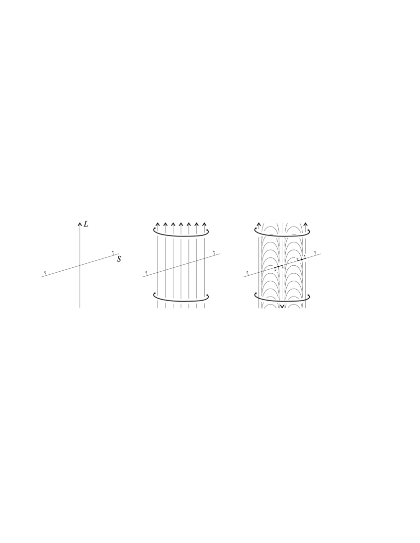
Figure 4: Effect of the Pontrjagin move.

of the move. The fields pictured both have a rotational symmetry, suggested in the figure. The two tangency points which arise are a positive focus (on the right) and a negative saddle (on the left), so the local contribution is indeed $+2$, and the proof is complete.  2.10

Remark 2.11

The definition of rotation number and Proposition 2.10 easily extend to the case of manifolds which are not homology spheres, by restricting to homologically trivial knots and choosing a relative homology class in the complement.

We can now prove that in a homology sphere all knots are good.

Proof of  2.5. Consider $[f]\in G(K)$, a framing $F$ on $K$ and $\xi\in{\rm Eul}(E(K),{\cal P}(K^{F}))$. We must show that $f_{*}(\xi)=\xi$. Let $\xi=[v]$ and denote by $\widehat{v}$ the obvious extension of $v$ to $M$. As above, let $\widehat{f}$ be the extension of $f$ to $M$. During the proof of Proposition 2.10 we have shown that

$${\rm rot}_{\widehat{f}_{*}(\widehat{v})}(K)-{\rm rot}_{\widehat{v}}(K)=2\alpha(f_{*}(v),v).$$

But ${\rm rot}_{\widehat{f}_{*}(\widehat{v})}(K)$ is actually equal to ${\rm rot}_{\widehat{v}}(K)$, because $\widehat{f}$ is the identity near $K$. Therefore $f_{*}(v)$ and $v$ differ by a torsion element of $H_{1}(E(K);{\hbox{\Bbb Z}})\cong{\hbox{\Bbb Z}}$, so they are equal. By definition $f_{*}(\xi)=[f_{*}(v)]$ and $\xi=[v]$, and the proof is complete.  2.5

Theorems 2.4 and 2.5 provide a partial answer to the problem of determining which knots are good. The general problem does not appear to be straight-forward, and we leave it for further investigation. We will only show below an example of knot which is not good.

Knots distinguished by torsion.

This paragraph is devoted to proving Theorem 0.1. Within the proof we will need the following general fact, which we state separately:

Lemma 2.12

Let $(v_{t})_{t\in[0,1]}$ be a homotopy of non-singular vector fields on a $3$-manifold $M$, and let $K_{0}$ be a knot transversal to $v_{0}$. Then $K_{0}$ extends to an isotopy $(K_{t})_{t\in[0,1]}$ such that $K_{t}$ is transversal to $v_{t}$ for all $t$.

This lemma can be established using the classical methods of general position and obstruction theory, and we leave it to the reader. We just mention that an easy alternative proof could also be given in the framework of the theory of branched standard spines, using Theorem 4.2 and ${\rm C}^{1}$ projections of knots (see [4]).

We state now our main result, addressing the reader to [9] for the definition of overtwisted contact structure. Before giving the proof we discuss the consequences which are most relevant to us.

Proposition 2.13

Let $(v,K)$ be a pseudo-Legendrian pair in $M$. For all

$$\gamma\in{\rm Ker}(i_{*}:H_{1}(E(K);{\hbox{\Bbb Z}})\to H_{1}(M;{\hbox{\Bbb Z}}))$$

there exists a pseudo-Legendrian knot $K_{\gamma}$ in $(M,v)$ and an isotopy $f:M\to M$ which maps $K_{\gamma}^{(v)}$ to $K^{(v)}$ such that

$$\alpha(\xi(v,K),f_{*}(\xi(v,K_{\gamma})))=\gamma.$$

Moreover, if $v$ is transversal to an assigned overtwisted contact structure $\eta$ and $K$ is Legendrian in $\eta$ then also $K_{\gamma}$ can be chosen to be Legendrian in $\eta$.

Remark 2.14

If $K^{(v)}$ is good and $\gamma\neq 0$, the pairs $(v,K)$ and $(v,K_{\gamma})$ are not weakly equivalent, and a torsion tells them apart, in the sense that Proposition 2.6 applies. (To see this, choose $\varphi:H_{1}(E(K);{\hbox{\Bbb Z}})\to\Lambda_{*}$ with $\varphi(\gamma)\neq 1$, consider the induced representation of $\pi_{1}(E(K))$, and apply formula (2) of Theorem 1.10.)

Remark 2.15

When $M$ is a homology sphere, so that $K$ is automatically good, the family of knots obtained from Proposition 2.13 is parameterized by ℤ, and we can choose a representation $\varphi:\pi_{1}(E(K))\to\Lambda_{*}$ such that $\tau^{\varphi}$ takes a different value on each knot of the family. This shows in particular that the knots are pairwise weakly inequivalent. In the contact case, the knots are pairwise framed-isotopic but not isotopic through Legendrian knots. (For a proof, choose $\varphi$ such that $\varphi(1)$ has infinite order.)

Proof of  2.13. We start by modifying the field $v$ on $E(K)$ to a field $w$, without modification near $\partial E(K)$, in such a way that $\alpha(v\big{|}_{E(K)},w)=\gamma\in H_{1}(E(K);{\hbox{\Bbb Z}})$. This can be achieved by a “Pontrjagin move”, as already used within the proof of 2.10. Let us spell out the steps to be followed:

1. Select an oriented link $L$ in the interior of $E(K)$ representing $\gamma\in H_{1}(E(K);{\hbox{\Bbb Z}})$;

2. Assume by general position that $v$ is transversal to $L$;

3. Replace $v$ by a new field $v^{\prime}$ which runs parallel to $L$ in a tubular neighbourhood $W(L)$ of $L$; note that $\alpha(v\big{|}_{E(K)},v^{\prime})=0\in H_{1}(E(K);{\hbox{\Bbb Z}})$;

4. Modify $v^{\prime}$ only within $W(L)$ to a field $w$ which runs opposite to $L$ on $L$ and has non-positive radial component on $W(L)$.

Our next step is to extend $w$ to a field $z$ on the whole of $M$, which we can do simply by defining $z$ to coincide with $v$ on $U(K)$. Since $\gamma$ is in the kernel, at the $H_{1}$-level, of the inclusion of $E(K)$ into $M$, the homotopy classes of $v$ and $z$ on $M$ differ at most by a Hopf number (i.e. they define the same Euler structure on $M$). Therefore we can select a ball $B$ contained in the interior of $E(K)$ and modify $z$ on $B$ to a new field $y$ such that the Hopf number of $y$ relative to $v$ is zero. The modification on $B$ is also a Pontrjagin move. Note now that $w$ and $y\big{|}_{E(K)}$ differ by a local modification, so they define the same Euler structure on $E(K)$. In particular $\alpha(v\big{|}_{E(K)},y\big{|}_{E(K)})=\gamma\in H_{1}(E(K);{\hbox{\Bbb Z}})$.

Now by construction $y$ and $v$ are homotopic on $M$ and $K$ is transversal to $y$. If $(v_{t})_{t\in[0,1]}$ is the homotopy, with $v_{0}=y$ and $v_{1}=v$, we can apply Proposition 2.12 and find a continuous family $(g_{t})_{t\in[0,1])}$ of diffeomorphisms of $M$ fixed on $\partial M$ with $g_{0}={\rm id}$ and $g_{t}(K)$ transversal to $v_{t}$ for all $t$. As in the proof of Proposition 2.2 the homology class

$$\alpha(\xi(v,K),g_{t}^{*}(\xi(v_{t},g_{t}(K))))$$

is constantly $\gamma$ because it is $\gamma$ at $t=0$. So it is sufficient to define $K_{\gamma}$ as $g_{1}(K)$ and $f$ as $g_{1}^{-1}$.

When $v$ is transversal to an overtwisted contact structure $\eta$, we fix a metric such that they are actually orthogonal, and we modify our proof as follows (assuming the reader is familiar with the techniques of Eliashberg, see [9]):

1. Instead of modifying $v\big{|}_{E(K)}$ to $w$ by a Pontrjagin move, we construct a new contact structure by application of a Lutz twist to $\eta\big{|}_{E(K)}$, so that the effect (up to homotopy) on the orthogonal vector field is the same as the original modification. Then we extend the structure near $K$ as obvious, calling $z$ its normal field.

2. Instead of modifying $z$ to $y$, again we use a Lutz twist on the normal contact structure. Moreover we make sure that $y^{\perp}$ is overtwisted by applying (if necessary) another Lutz twist of the sort which does not change the homotopy class, away from $K$.

3. We conclude using Eliashberg’s classification of overtwisted structures, according to which two such structures which are homotopic as plane fields are automatically isotopic.

The proof is complete.  2.13

Remark 2.16

A more constructive proof of the contact version of Proposition 2.13 may be given in the framework of [3]. On the other hand, the proof we have given above raises the following natural question: assume $\eta_{0}$ and $\eta_{1}$ are overtwisted contact structures on $M$, let $L_{0}$ and $L_{1}$ be links tangent to $\eta_{0}$ and $\eta_{1}$ respectively, and assume there exist a family $(\eta_{t},L_{t})_{t\in[0,1]}$ where $(\eta_{t})$ is a homotopy of plane fields, $(L_{t})$ is an isotopy, and $L_{t}$ is tangent to $\eta_{t}$. Can this family be replaced by a similar one where $(\eta_{t})$ is an isotopy? Eliashberg’s classification theorem may be stated as “yes, for $L_{0}=\emptyset$”, and a general proof could possibly be obtained along the lines of [9]. Should the answer be “yes, for any $L_{0}$”, we would have a bijection between pseudo-Legendrian links (up to weak equivalence) and Legendrian links in overtwisted structures (up to Legendrian isotopy).

Curls and winding number.

We show in this paragraph that torsions are sensitive to an analogue of the winding number (the invariant which allows to distinguish framed-isotopic link projections which are not equivalent under the second and third of Reidemeister’s moves, see [25]). This will allow us to give another recipe, besides Proposition 2.13, to construct knots which are distinguished by torsion. Moreover we will give an example of knot which is not good. The proof of the next result uses the example of Section 5, so it is deferred to Section 6.

Proposition 2.17

Consider a field $v$ on $M$ and a portion of $M$ on which $v$ can be identified to the vertical field in ${\hbox{\Bbb R}}^{3}$. Consider knots $K_{0}$ and $K_{1}$ which are transversal to $v$ and differ only within the chosen portion of $M$, as shown in Fig. 5.

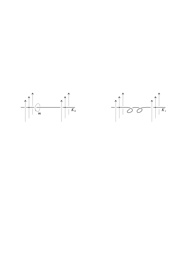
Figure 5: Knots which differ for the winding number.

Choose a meridian $m$ of $K_{0}$ as also shown in the figure. Let $f$ be an isotopy which maps $K_{1}^{(v)}$ to $K_{0}^{(v)}$ and is supported in a tubular neighbourhood of $K_{0}$. Then:

$$\alpha(\xi(v,K_{0}),f_{*}(\xi(v,K_{1})))=[m]\in H_{1}(E(K_{0});{\hbox{\Bbb Z}}).$$

Proposition 2.18

Let $(v,K_{0})$ be a pseudo-Legendrian pair in $M$, and denote by $[m]\in H_{1}(E(K_{0});{\hbox{\Bbb Z}})$ the homology class of the meridian of $U(K_{0})$. Assume either that $K_{0}^{(v)}$ is good and $[m]\neq 0$ or that $E(K_{0})$ is hyperbolic and $[m]$ has infinite order. Let $K_{1}$ be a knot obtained from $K_{0}$ as in Fig. 5. Then $(v,K_{0})$ and $(v,K_{1})$ are not weakly equivalent.

Proof of  2.18. By contradiction, using Propositions 2.2 and 2.17, we would get elements $\xi_{0},\xi_{1}$ of ${\rm Eul}(E(K_{0}),{\cal P}(K_{0}^{(v)})$ such that $\alpha(\xi_{0},\xi_{1})=[m]$ and $\xi_{1}=f_{*}(\xi_{0})$ for some $[f]\in G(K_{0})$. If $K_{0}^{(v)}$ is good and $[m]\neq 0$ this is a contradiction. Assume now that $E(K_{0})$ is hyperbolic and $[m]$ has infinite order. Since $f_{*}([m])=[m]$, using Lemma 2.9 we easily see that $\alpha(\xi_{0},f_{*}^{k}(\xi_{0}))=k\cdot[m]$ for all $k$. Proposition 2.8 and the result of Johansson already used in the proof of Theorem 2.4 now imply that $f^{k}$ acts trivially on ${\rm Eul}(E(K_{0}),{\cal P}(K_{0}^{(v)})$ for some $k$, whence the contradiction.  2.18

As an application of Proposition 2.17, we can show that there exist knots which are not good. Consider $S^{2}\times[0,1]$ with vector field parallel to the $[0,1]$ factor. Let $K_{0}$ be the equator of $S^{2}\times\{1/2\}$, and let $K_{1}$ be obtained from $K_{0}$ by the modification described in Fig. 5. Using Proposition 2.17, if we choose a framed-isotopy $g$ of $K_{1}^{(v)}$ onto $K_{0}^{(v)}$ supported in $U(K_{0})$, we have

$$\alpha(\xi(v,K_{0}),(g\big{|}_{E(K_{1})})_{*}(\xi(v,K_{1})))=[m],$$

where $[m]$ is a generator of $H_{1}(E(K_{0});{\hbox{\Bbb Z}})\cong{\hbox{\Bbb Z}}$. On the other hand, $K_{1}$ is strongly equivalent to $K_{0}$ in $(M,v)$ (the winding number only exists on ${\hbox{\Bbb R}}^{2}$, not on $S^{2}$). So there exists an isotopy $h$ of $K_{1}^{(v)}$ onto $K_{0}^{(v)}$ through links transversal to $v$, and we have

$$\alpha(\xi(v,K_{0}),(h\big{|}_{E(K_{1})})_{*}(\xi(v,K_{1})))=0.$$

This implies that $(h\,{\scriptstyle\circ}\,g^{-1})\big{|}_{E(K_{0})}$ acts non-trivially on $\xi(v,K_{0})\in{\rm Eul}(E(K_{0}),{\cal P}(K_{0}^{(v)}))$.

3 Torsion of a convex combinatorial Euler structure

In this section we formally define torsion. Fix a manifold $M$, a convex boundary pattern ${\cal P}=(W,B,V,\emptyset)$ on $M$, a cellularization ${\cal C}$ suited to ${\cal P}$ and a representation $\varphi:\pi_{1}(M)\to\Lambda_{*}$, where $\Lambda$ is as mentioned before the statement of Theorem 1.10. We will denote by $\varphi$ again the extension ${\hbox{\Bbb Z}}[\pi_{1}(M)]\to\Lambda$ (a ring homomorphism).

We consider now the universal cover $q:\tilde{M}\to M$ and the twisted chain complex ${\rm C}^{\varphi}_{*}(M,W\cup V)$, where ${\rm C}^{\varphi}_{i}(M,W\cup V)$ is defined as $\Lambda\otimes_{\varphi}{\rm C}^{\rm cell}_{i}(\tilde{M},q^{-1}(W\cup V);{\hbox{\Bbb Z}})$, and the boundary operator is induced from the ordinary boundary. The homology of this complex is denoted by $H^{\varphi}_{*}(M,W\cup V)$ and called the $\varphi$-twisted homology. We assume that each $H^{\varphi}_{i}(M,W\cup V)$ is a free $\Lambda$-module and fix a basis ${\hbox{\Got h}}_{i}$.

Remark 3.1

1. To have a formal completely intrinsic definition of $H^{\varphi}_{*}(M,W\cup V)$, one should fix from the beginning a basepoint $x_{0}\in M$ for $\pi_{1}(M)$, and consider pointed universal covers $q:(\tilde{M},\tilde{x}_{0})\to(M,x_{0})$, because any two such covers are canonically isomorphic, and the action of $\pi_{1}(M)$ on $\tilde{M}$ is canonically defined on them.

2. To define $H^{\varphi}_{*}(M,W\cup V)$ we have used in an essential way the fact that $W\cup V=\overline{W}$ is closed, because otherwise ${\rm C}^{\varphi}_{*}(M,W\cup V)$ cannot be defined.

3. ${\rm C}^{\varphi}_{i}(M,W\cup V)$ is a free $\Lambda$-module, and each ${\hbox{\Bbb Z}}[\pi_{1}(M)]$-basis of ${\rm C}^{\rm cell}_{i}(\tilde{M},q^{-1}(W\cup V);{\hbox{\Bbb Z}})$ determines a $\Lambda$-basis of ${\rm C}^{\varphi}_{i}(M,W\cup V)$.

4. If we compose $\varphi$ with the projection $\Lambda_{*}\to{\overline{K}}_{1}(\Lambda)$ we get a homomorphism of $\pi_{1}(M)$ into an Abelian group, so we get a homomorphism $\overline{\varphi}:H_{1}(M;{\hbox{\Bbb Z}})\to{\overline{K}}_{1}(\Lambda).$

Now let $\xi\in{\rm Eul}^{\rm c}(M,{\cal P})$ and choose a representative of $\xi$ as in point 2 of Proposition 1.4, namely

$$\sum_{\sigma\in{\cal C},\ \sigma\subset M\setminus(W\cup V)}{\rm ind}(\sigma)\cdot\beta_{\sigma}$$

with $\beta_{\sigma}(0)=x_{0}$ for all $\sigma$, $x_{0}$ being a fixed point of $M$. We choose $\tilde{x}_{0}\in q^{-1}(x_{0})$ and consider the liftings $\tilde{\beta}_{\sigma}$ which start at $\tilde{x}_{0}$. For $\sigma\subset M\setminus(W\cup V)$ we select its preimage $\tilde{\sigma}$ which contains $\tilde{\beta}_{\sigma}(1)$, and define ${\hbox{\Got g}}(\xi)$ as the collection of all these $\tilde{\sigma}$. Arranging the $i$-dimensional elements of ${\hbox{\Got g}}(\xi)$ in any order, by Remark 3.1(3) we get a $\Lambda$-basis ${\hbox{\Got g}}_{i}(\xi)$ of ${\rm C}^{\varphi}_{i}(M,W\cup V)$. We consider a set ${\tilde{\hbox{\Got h}}}_{i}$ of elements of ${\rm C}^{\varphi}_{i}(M,W\cup V)$ which project to the fixed basis ${\hbox{\Got h}}_{i}$ of $H^{\varphi}_{i}(M,W\cup V)$.

Now note that, given a free $\Lambda$-module $L$ and two finite bases ${\hbox{\Got b}}=(b_{k})$, ${\hbox{\Got b}}^{\prime}=(b^{\prime}_{k})$ of $M$, the assumption made on $\Lambda$ guarantees that b and ${\hbox{\Got b}}^{\prime}$ have the same number of elements, so there exists an invertible square matrix $(\lambda^{h}_{k})$ such that $b^{\prime}_{k}=\sum_{h}\lambda^{h}_{k}b_{h}$. We will denote by $[{\hbox{\Got b}}^{\prime}/{\hbox{\Got b}}]$ the image of $(\lambda^{h}_{k})$ in $K_{1}(\Lambda)$ (see Section 1 for the definition).

Proposition 3.2

If ${\hbox{\Got b}}_{i}\subset{\rm C}^{\varphi}_{i}(M,W\cup V)$ is such that $\partial{\hbox{\Got b}}_{i}$ is a $\Lambda$-basis of $\partial({\rm C}^{\varphi}_{i}(M,W\cup V))$, then $(\partial{\hbox{\Got b}}_{i+1})\cdot\tilde{\hbox{\Got h}}_{i}\cdot{\hbox{\Got b}}_{i}$ is a $\Lambda$-basis of ${\rm C}^{\varphi}_{i}(M,W\cup V)$, and

$$\tau^{\varphi}(M,{\cal P},\xi,{\hbox{\Got h}})=\pm\prod_{i=0}^{3}\Big{[}\Big{(}(\partial{\hbox{\Got b}}_{i+1})\cdot\tilde{\hbox{\Got h}}_{i}\cdot{\hbox{\Got b}}_{i}\Big{)}\;\Big{/}\;{\hbox{\Got g}}_{i}(\xi)\Big{]}^{(-1)^{i}}\in{\overline{K}}_{1}(\Lambda)$$

is independent of all choices made. Moreover

$$\tau^{\varphi}(M,{\cal P},\xi^{\prime},{\hbox{\Got h}})=\tau^{\varphi}(M,{\cal P},\xi,{\hbox{\Got h}})\cdot\overline{\varphi}(\alpha^{\rm c}(\xi^{\prime},\xi)).$$ (4)

Proof of  3.2. The first assertion and independence of the ${\hbox{\Got b}}_{i}$’s is purely algebraic and classical, see [21]. Now note that $\xi\in{\rm Eul}^{\rm c}(M,{\cal P})$ was used to select the bases ${\hbox{\Got g}}_{i}(\xi)$. The ${\hbox{\Got g}}_{i}(\xi)$ are of course not uniquely determined themselves, but we can show that different choices lead to the same value of $\tau^{\varphi}$.

First of all, the arbitrary ordering in the ${\hbox{\Got g}}_{i}(\xi)$ is inessential because torsion is only regarded up to sign. Second, consider the effect of choosing a different representative of $\xi$. This leads to a new family $\tilde{\sigma}^{\prime}$ of cells. If $\tilde{\sigma}^{\prime}=a(\sigma)\cdot\tilde{\sigma}$, with $a(\sigma)\in\pi_{1}(M)$, and $\overline{a}(\sigma)$ is the image in $H_{1}(M;{\hbox{\Bbb Z}})$, we automatically have

$$\sum_{\sigma\subset M\setminus{W\cup V}}{\rm ind}(\sigma)\cdot\overline{a}(\sigma)=0\in H_{1}(M;{\hbox{\Bbb Z}}),$$

which allows to conclude that also the representative chosen is inessential. The choice of the lifting $\tilde{x}_{0}$ can be shown to be inessential either in the spirit of Remark 3.1(1), or by showing that a simultaneous $a$-translation of all $\tilde{\sigma}$, for $a\in\pi_{1}(M)$, multiplies the torsion by $\overline{\varphi}(a)^{\chi(M)-\chi(W\cup V)}=1$.

Formula (4) is readily established by choosing representatives $\sum{\rm ind}(\sigma)\cdot\beta_{\sigma}$ and $\sum{\rm ind}(\sigma)\cdot\beta^{\prime}_{\sigma}$ of $\xi$ and $\xi^{\prime}$ such that $\beta^{\prime}_{\sigma}=\beta_{\sigma}$ for all $\sigma$ but one.  3.2

Since the above construction uses the cellularization ${\cal C}$ in a way which may appear to be essential, we add a subscript ${\cal C}$ to the torsion we have defined. The next result, which can be established following Turaev [27], shows that dependence on ${\cal C}$ is actually inessential. Together with Theorem 1.5 and Propositions 1.4 and 3.2, it concludes the proof of Theorem 1.10.

Proposition 3.3

Let ${\cal C}$ and ${\cal C}^{\prime}$ be cellularizations suited to ${\cal P}$. Assume that ${\cal C}^{\prime}$ subdivides ${\cal C}$, and consider the bijection ${\cal S}_{({\cal C}^{\prime},{\cal C})}:{\rm Eul}^{\rm c}(M,{\cal P})_{\cal C}\to{\rm Eul}^{\rm c}(M,{\cal P})_{{\cal C}^{\prime}}$ of Proposition 1.4, and the canonical isomorphism $j_{({\cal C}^{\prime},{\cal C})}:H^{\varphi}_{*}(M,W\cup V)_{\cal C}\to H^{\varphi}_{*}(M,W\cup V)_{{\cal C}^{\prime}}$. Then, with obvious meaning of symbols we have:

$$\tau^{\varphi}_{\cal C}(M,{\cal P},\xi,{\hbox{\Got h}})=\tau^{\varphi}_{{\cal C}^{\prime}}(M,{\cal P},{\cal S}_{({\cal C}^{\prime},{\cal C})}(\xi),j_{({\cal C}^{\prime},{\cal C})}({\hbox{\Got h}})).$$

It is maybe appropriate here to remark that the choice of a basis h of $H^{\varphi}_{*}(M,W\cup V)$ and the definition of $\tau^{\varphi}(M,{\cal P},\xi,{\hbox{\Got h}})$ implicitly assume a description of the universal cover of $M$, which is typically undoable in practical cases. However, if one starts from a representation of $\pi_{1}(M)$ into the units of a commutative ring $\Lambda$, i.e. a representation which factors through one of $H_{1}(M;{\hbox{\Bbb Z}})$, one can use from the very beginning the maximal Abelian rather than the universal cover, which makes computations more feasible.

Remark 3.4

Turaev [26] has shown that a homological orientation yields a sign-refinement of torsion, i.e. a lifting from ${\overline{K}}_{1}(\Lambda)$ to $K_{1}(\Lambda)$. This refinement extends with minor modifications to our setting of boundary tangency. This sign-refinement, in the closed and monochromatic case, is an essential component of the theory (for instance, it is crucial for the relation with the 3-dimensional Seiberg-Witten invariants [28], [29] and for the definition of the Casson invariant [15]), so we expect it to be relevant also in the boundary pattern case.

Computation of torsion via disconnected spiders.

In this paragraph we show that to determine the family of lifted cells necessary to define torsion one can use representatives of Euler structures more general than those used above. This is a technical point which we will use below to compute torsions using branched spines (Section 4).

We fix $M$, ${\cal P}$, ${\cal C}$ and $\varphi$ as above, and $\xi\in{\rm Eul}^{\rm c}(M,{\cal P})$. Let ${\hbox{\Got g}}(\xi)=\{\tilde{\sigma}\}$ be the family of liftings of the cells lying in $M\setminus(W\cup V)$ determined by a connected spider as explained above. Note that if ${\hbox{\Got g}}^{\prime}=\{\tilde{\sigma}^{\prime}\}$ is any other family of liftings we have $\tilde{\sigma}^{\prime}=a(\sigma)\cdot\tilde{\sigma}$ for some $a\in\pi_{1}(M)$, and we can define

$$h({\hbox{\Got g}}^{\prime},{\hbox{\Got g}}(\xi))=\sum_{\sigma\subset M\setminus(W\cup V)}{\rm ind}(\sigma)\cdot\overline{a}(\sigma)\in H_{1}(M;{\hbox{\Bbb Z}}).$$

Proposition 3.5

Assume there exists a partition ${\cal C}_{1}\sqcup\dots\sqcup{\cal C}_{k}$ of the set of cells lying in $M\setminus(W\cup V)$, and let $\xi\in{\rm Eul}^{\rm c}(M,{\cal P})$ have a representative of the form

$$z=\sum_{j=1}^{k}\left(\sum_{\sigma\in{\cal C}_{j}\setminus\{\sigma_{j}\}}{\rm ind}(\sigma)\cdot\gamma^{(j)}_{\sigma}\right)$$

where $\sigma_{j}\in{\cal C}_{j}$ and $\gamma^{(j)}_{\sigma}:([0,1],0,1)\to(M,p_{\sigma_{j}},p_{\sigma})$. Choose any lifting $\tilde{p}_{\sigma_{j}}$ of $p_{\sigma_{j}}$, lift $\gamma^{(j)}_{\sigma}$ to $\tilde{\gamma}^{(j)}_{\sigma}$ starting from $\tilde{p}_{\sigma_{j}}$, let $\tilde{\sigma}^{\prime}$ be the lifting of $\sigma$ containing $\tilde{\gamma}^{(j)}_{\sigma}(1)$, and let ${\hbox{\Got g}}^{\prime}$ be the family of all these liftings. Then $h({\hbox{\Got g}}^{\prime},{\hbox{\Got g}}(\xi))=0\in H_{1}(M;{\hbox{\Bbb Z}})$. In particular ${\hbox{\Got g}}^{\prime}$ can be used to compute $\tau^{\varphi}(M,{\cal P},\xi,{\hbox{\Got h}})$.

Proof of  3.5. Note first that the coefficient of $p_{\sigma_{j}}$ in $\partial z$ is exactly

$$-\sum_{\sigma\in{\cal C}_{j}\setminus\{\sigma_{j}\}}{\rm ind}(\sigma).$$

On the other hand this coefficient must be equal to ${\rm ind}(\sigma_{j})$. Summing up we deduce that $\sum_{\sigma\in{\cal C}_{j}}{\rm ind}(\sigma)=0$.

Now choose $x_{0}\in M$ and $\delta^{(j)}:([0,1],0,1)\to(M,x_{0},p_{\sigma_{j}})$. For $\sigma\in{\cal C}_{j}$ define

$$\beta_{\sigma}=\cases{\delta^{(j)}&if $\sigma=\sigma_{j}$\cr\delta^{(j)}\cdot\gamma^{(j)}_{\sigma}&otherwise,}$$

so that $\beta_{\sigma}:([0,1],0,1)\to(M,x_{0},p_{\sigma})$, whence $w=\sum_{\sigma\subset M\setminus(W\cup V)}\beta_{\sigma}$ is an Euler chain. Moreover:

$$w-z=\sum_{j=1}^{k}\left(\sum_{\sigma\in{\cal C}_{j}}{\rm ind}(\sigma)\right)\cdot\delta^{(j)}=0\in H_{1}(M;{\hbox{\Bbb Z}}),$$

so $[w]=\xi$. Now choose $\tilde{x}_{0}$ over $x_{0}$, lift the $\delta^{(j)}$ and $\beta_{\sigma}$ starting from $\tilde{x}_{0}$, and let $a^{(j)}\in\pi_{1}(M)$ be such that $\tilde{p}_{\sigma_{j}}=a^{(j)}\cdot\tilde{\delta}^{(j)}(1)$. Then

$$h({\hbox{\Got g}}^{\prime},{\hbox{\Got g}}(\xi))=\sum_{j=1}^{k}\left(\sum_{\sigma\in{\cal C}_{j}}{\rm ind}(\sigma)\right)\cdot\overline{a}^{(j)}=0\in H_{1}(M;{\hbox{\Bbb Z}}),$$

and the proof is complete.  3.5

4 Spines and computation of torsion

In this section we show how to compute torsions starting from a combinatorial encoding of vector fields. We first review the theory developed in [2]. See the beginning of Section 1 for our conventions on manifolds, maps, and fields. In addition to the terminology introduced there, we will need the notion of traversing field on a manifold $M$, defined as a field whose orbits eventually intersect $\partial M$ transversely in both directions (in other words, orbits are compact intervals).

Branched spines.

A simple polyhedron $P$ is a finite connected 2-dimensional polyhedron with singularity of stable nature (triple lines and points where six non-singular components meet). Such a $P$ is called standard if all the components of the natural stratification given by singularity are open cells. Depending on dimension, we will call the components vertices, edges and regions.

A standard spine of a $3$-manifold $M$ with $\partial M\neq\emptyset$ is a standard polyhedron $P$ embedded in ${\rm Int}(M)$ so that $M$ collapses onto $P$. Standard spines of oriented $3$-manifolds are characterized among standard polyhedra by the property of carrying an orientation, defined (see Definition 2.1.1 in [2]) as a “screw-orientation” along the edges (as in the left-hand-side of Fig. 6), with an obvious compatibility at vertices (as in the centre of Fig. 6).

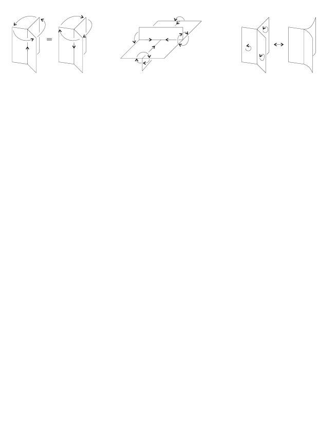
Figure 6: Convention on screw-orientations, compatibility at vertices, and geometric interpretation of branching.

It is the starting point of the theory of standard spines that every oriented $3$-manifold $M$ with $\partial M\neq\emptyset$ has an oriented standard spine, and can be reconstructed (uniquely up to homeomorphism) from any of its oriented standard spines. See [7] for the non-oriented version of this result and [1] or Proposition 2.1.2 in [2] for the (slight) oriented refinement.

A branching on a standard polyhedron $P$ is an orientation for each region of $P$, such that no edge is induced the same orientation three times. See the right-hand side of Fig. 6 and Definition 3.1.1 in [2] for the geometric meaning of this notion. An oriented standard spine $P$ endowed with a branching is shortly named branched spine. We will never use specific notations for the extra structures: they will be considered to be part of $P$. The following result, proved as Theorem 4.1.9 in [2], is the starting point of our constructions.

Proposition 4.1

To every branched spine $P$ there corresponds a manifold $M(P)$ with non-empty boundary and a concave traversing field $v(P)$ on $M(P)$. The pair $(M(P),v(P))$ is well-defined up to diffeomorphism. Moreover an embedding $i:P\to{\rm Int}(M(P))$ is defined, and has the property that $v(P)$ is positively transversal to $i(P)$.

The topological construction which underlies this proposition is actually quite simple, and it is illustrated in Fig. 7. Concerning the last

Figure 7: Manifold and field associated to a branched spine.

assertion of the proposition, note that the branching allows to define an oriented tangent plane at each point of $P$.

Combinatorial encoding of combings.

Let $P$ be a branched spine, and define $v(P)$ on $M(P)$ as just explained. Assume that in $\partial M(P)$ there is only one component which is homeomorphic to $S^{2}$ and is split by the tangency line of $v(P)$ to $\partial M(P)$ into two discs. (Such a component will be denoted by $S^{2}_{\rm triv}$.) Now, notice that $S^{2}_{\rm triv}$ is also the boundary of the closed $3$-ball with constant vertical field, denoted by $B^{3}_{\rm triv}$. This shows that we can cap off $S^{2}_{\rm triv}$ by attaching a copy of $B^{3}_{\rm triv}$, getting a compact manifold ${\widehat{M}}(P)$ and a field ${\widehat{v}}(P)$ on ${\widehat{M}}(P)$. If we denote by ${\widehat{{\cal P}}}(P)$ the boundary pattern of ${\widehat{v}}(P)$ on ${\widehat{M}}(P)$, we easily see that the pair $({\widehat{M}}(P),{\widehat{v}}(P))$ is only well-defined up to homeomorphism of ${\widehat{M}}(P)$ and homotopy of ${\widehat{v}}(P)$ through fields compatible with ${\widehat{{\cal P}}}(P)$. Note also that ${\widehat{{\cal P}}}(P)$ is automatically concave.

If ${\cal P}$ is a boundary pattern on $M$, we define ${\rm Comb}(M,{\cal P})$ as the set of fields compatible with ${\cal P}$ under homotopy through fields also compatible with ${\cal P}$. An element of ${\rm Comb}(M,{\cal P})$ is called a combing on $(M,{\cal P})$. Note that we have a projection ${\rm Comb}(M,{\cal P})\to{\rm Eul}(M,{\cal P})$.

The above construction shows that a branched spine $P$ with only one $S^{2}_{\rm triv}$ on $\partial M(P)$ defines an element $\Phi(P)$ of ${\rm Comb}({\widehat{M}}(P),{\widehat{{\cal P}}}(P))$. One of the main achievements of [2] (Theorems 1.4.1 and 5.2.1) is the following.

Theorem 4.2

1. If $M$ is a closed oriented $3$-manifold, $\Phi$ maps surjectively the set $\{P:{\widehat{M}}(P)\cong M\}$ onto ${\rm Comb}(M)={\rm Comb}(M,\emptyset)$.

2. A finite list of local combinatorial moves on branched spines can be given so that if ${\widehat{M}}(P_{0})\cong{\widehat{M}}(P_{1})\cong M$ is closed and $\Phi(P_{0})=\Phi(P_{1})\in{\rm Comb}(M)$, then $P_{1}$ is obtained from $P_{0}$ by a finite sequence of these moves.

In the present paper we will not use the moves referred to in the previous statement, but to give the reader an idea of their geometric meaning we quickly picture them. The complete list actually consists of 18 moves, but the essential “physical” phenomena which occur are only those shown in Fig. 8 (the other moves are obtained by taking mirrors of those shown).

Figure 8: Moves for branched standard spines.

In [4] we will show that the rightmost move in Fig. 8 is actually implied by the other moves, and we will establish the following extension of Theorem 4.2.

Theorem 4.3

1. If $M$ is any compact oriented $3$-manifold and ${\cal P}$ is a concave boundary pattern on $M$ not containing $S^{2}_{\rm triv}$ components, then $\Phi$ maps surjectively $\{P:\ {\widehat{M}}(P)\cong M,\ {\widehat{{\cal P}}}(P)\cong{\cal P}\}$ onto ${\rm Comb}(M,{\cal P})$.

2. The same finite list of moves as in point 2 of Theorem 4.2 has the property that if $({\widehat{M}}(P_{0}),{\widehat{{\cal P}}}(P_{0}))\cong({\widehat{M}}(P_{1}),{\widehat{{\cal P}}}(P_{1}))\cong(M,{\cal P})$ is as above and $\Phi(P_{0})=\Phi(P_{1})\in{\rm Comb}(M,{\cal P})$, then $P_{1}$ is obtained from $P_{0}$ by a finite sequence of these moves.

The proof of this result requires considerable technicalities, so we have decided to omit it here, also because point 2 is not used, and point 1 is only needed to show that the recipe we will give to compute torsions actually allows to compute all concave torsions. We just mention that both points are established by extending to the bounded case the notion of normal section of a field, introduced in [13] and [2] (Section 5.1). The following geometric interpretation of point 1 may be of some interest.

Remark 4.4

In general, the dynamics of a field, even a concave one, can be very complicated, whereas the dynamics of a traversing field (in particular, $B^{3}_{\rm triv}$) is simple. Point 1 in Theorem 4.3 means that for any (complicated) concave field there exists a sphere $S^{2}$ which splits the field into two (simple) pieces: a standard $B^{3}_{\rm triv}$ and a concave traversing field.

Another reason for not proving point 1 of Theorem 4.3 in general is that we can give an easy special proof for the case we are most interested in, namely link complements. Note that our argument relies on Theorem 4.2 (and its proof).

Proof of point 1 of Theorem 4.3 for link complements. We have to show that if $M$ is closed, $v$ is a field on $M$ and $L$ is transversal to $v$, then the complement $E(L)$ of $L$ with the restricted field is represented by some branched spine in the sense explained above.

The construction explained in Section 5.1 of [2] shows that there exists a branched standard spine $P$ such that $v$ is positively transversal to $P$ and the complement of $P$, with the restriction of $v$, is isomorphic to the open 3-ball with the constant vertical field. The last condition easily implies that $L$ can be isotoped through links transversal to $v$ to a link lying in an arbitrarily small neighbourhood of $P$, with the further property that its natural projection on $P$ is ${\rm C}^{1}$, possibly with crossings. This fact is the starting point of a treatment of framed links via ${\rm C}^{1}$ projections on spines, which we plan to develop in [4].

Once $L$ has been isotoped to a ${\rm C}^{1}$ link on $P$, a branched spine of $(E(L),v\big{|}_{E(L)})$ is obtained by digging a tunnel in $P$ along the projection of $L$, as shown in Fig. 9.

Figure 9: How to dig a tunnel in a spine.

A crossing in the projection will of course give rise to 4 vertices in the spine. Note that the spine which results from the digging may occasionally be non-standard, but it is standard as soon as the projection is complicated enough (e.g. if on each component there are both a crossing and an intersection with $S(P)$).  4.3(1)$E(L)$

Remark 4.5

Using the fact that all the regions of a branched spine $P$ have non-empty boundary one can show quite easily that a link $L$ with ${\rm C}^{1}$ projection on $P$ can be isotoped through links transversal to $v(P)$ to a link whose projection does not have crossings. An example of how to get

Figure 10: Removing a crossing from a ${\rm C}^{1}$-projection.

rid of a crossing is given in Fig. 10.

Spines and ideal triangulations.

We remind the reader that an ideal triangulation of a manifold $M$ with non-empty boundary is a partition ${\cal T}$ of ${\rm Int}(M)$ into open cells of dimensions 1, 2 and 3, induced by a triangulation ${\cal T}^{\prime}$ of the space $Q(M)$, where:

1. $Q(M)$ is obtained from $M$ by collapsing each component of $\partial M$ to a point;

2. ${\cal T}^{\prime}$ is a triangulation only in a loose sense, namely self-adjacencies and multiple adjacencies of tetrahedra are allowed;

3. The vertices of ${\cal T}^{\prime}$ are precisely the points of $Q(M)$ which correspond to components of $\partial M$.

It turns out (see for instance [17], [22], [19]) that there exists a natural bijection between standard spines and ideal triangulations of a 3-manifold. Given an ideal triangulation, the corresponding standard spine is just the 2-skeleton of the dual cellularization, as illustrated in Figure 11.

Figure 11: Duality between standard spines and ideal triangulations.

The inverse of this correspondence will be denoted by $P\mapsto{\cal T}(P)$.

Now let $P$ be a branched spine. First of all, we can realize ${\cal T}(P)$ in such a way that its edges are orbits of the restriction of $v(P)$ to ${\rm Int}(M(P))$, and the 2-faces are unions of such orbits. Being orbits, the edges of ${\cal T}(P)$ have a natural orientation, and the branching condition, as remarked in [11], is equivalent to the fact that on each tetrahedron of ${\cal T}(P)$ exactly one of the vertices is a sink and one is a source.

Remark 4.6

It turns out that if $P$ is a branched spine, not only the edges, but also the faces and the tetrahedra of ${\cal T}(P)$ have natural orientations. For tetrahedra, we just restrict the orientation of $M(P)$. For faces, we first note that the edges of $P$ have a natural orientation (the prevailing orientation induced by the incident regions). Now, we orient a face of ${\cal T}(P)$ so that the algebraic intersection in $M(P)$ with the dual edge is positive.

Euler chain defined by a branched spine.

We fix in this paragraph a standard spine $P$ and consider its manifold $M=M(P)$. We start by noting that the ideal triangulation ${\cal T}={\cal T}(P)$ defined by $P$ can be interpreted as a realization of ${\rm Int}(M)$ by face-pairings on a finite set of tetrahedra with vertices removed. If, instead of removing vertices, we remove open conic neighbourhoods of the vertices, thus getting truncated tetrahedra, after the face-pairings we obtain $M$ itself. This shows that $P$ determines a cellularization $\overline{{\cal T}}=\overline{{\cal T}}(P)$ of $M$ with vertices only on $\partial M$ and 2-faces which are either triangles contained in $\partial M$ or hexagons contained in ${\rm Int}(M)$, with edges contained alternatively in $\partial M$ and in ${\rm Int}(M)$.

Now assume that $P$ is branched and that $\partial M$ contains only one $S^{2}_{\rm triv}$ component, so ${\widehat{M}}={\widehat{M}}(P)$ is defined. Note that ${\widehat{M}}$ can be thought of as the space obtained from $M$ by contracting $S^{2}_{\rm triv}$ to a point, so a projection $\pi:M\to{\widehat{M}}$ is defined, and $\pi(\overline{{\cal T}})$ is a cellularization of ${\widehat{M}}$. Next, we modify $\pi(\overline{{\cal T}})$ by subdividing the triangles on $\partial{\widehat{M}}$ as shown in Fig. 12.

Figure 12: Truncated tetrahedra and subdivision of the triangles on the boundary

The result is a cellularization ${\widehat{{\cal T}}}={\widehat{{\cal T}}}(P)$ of ${\widehat{M}}$. Note that ${\widehat{{\cal T}}}$ on $\partial{\widehat{M}}$ consists of “kites”, with long edges coming from tetrahedra and short edges coming from subdivision. Note also that ${\widehat{{\cal T}}}$ has exactly one vertex $x_{0}$ in ${\rm Int}({\widehat{M}})$, and that the cells contained in ${\rm Int}({\widehat{M}})$, except $x_{0}$, are the duals to the cells of the natural cellularization ${\cal U}={\cal U}(P)$ of $P$. For $u\in{\cal U}$ we denote by $\hat{u}$ its dual and by $p_{u}=p_{\hat{u}}$ the point where $u$ and $\hat{u}$ intersect, called the centre of both.

We will now use the field ${\widehat{v}}={\widehat{v}}(P)$ to construct a combinatorial Euler chain on ${\widehat{M}}$ with respect to ${\widehat{{\cal T}}}$. It is actually convenient to consider, instead of ${\widehat{v}}$, the field ${\overline{v}}=\pi(v)$, which coincides with ${\widehat{v}}$ except near $x_{0}$, where it has a (removable) singularity. For $u\in{\cal U}$ we denote by $\beta_{u}$ the arc obtained by integrating ${\overline{v}}(P)$ in the positive direction, starting from $p_{u}$, until the boundary or the singularity is reached. We define:

$$s(P)=\sum_{u\in{\cal U}}{\rm ind}(u)\cdot\beta_{u}.$$

Let us consider now the pattern ${\widehat{{\cal P}}}={\widehat{{\cal P}}}(P)=(W,B,\emptyset,C)$ defined by $P$. If $p$ is a vertex of $\pi(\overline{{\cal T}})$ contained in $B$, we define its star ${\rm St}(p)$ as the sum of the straight segments going from $p$ to the centres of all the kites containing $p$, minus the sum of the straight segments going from $p$ to the centres of all the long edges containing $p$. If $\sigma$ is an edge of $\pi(\overline{{\cal T}})$ contained in $B$ we define its bi-arrow ${\rm Ba}(\sigma)$ as the sum of the two straight segments going from the centre $p_{\sigma}$ of $\sigma$ to the centres of the two short kite-edges containing $p_{\sigma}$. A star and a bi-arrow are shown in Fig. 13.

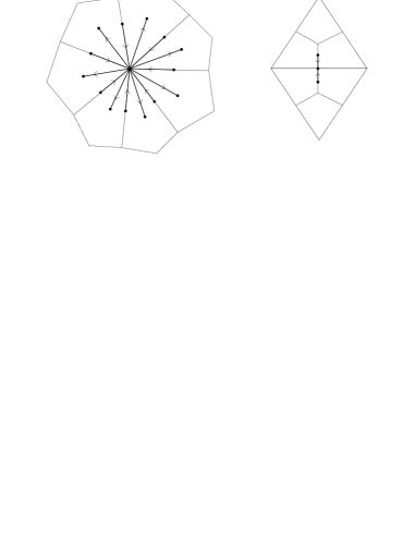
Figure 13: The star ${\rm St}(p)$ centred at a vertex $p$ contained in $B$ and the bi-arrow ${\rm Ba}(\sigma)$ based at the midpoint of an edge $\sigma$ contained in $B$

We define:

$$s^{\prime}(P)=s(P)+\sum_{p\in B\cap\overline{{\cal T}}(P)^{(0)}}{\rm St}(p)+\sum_{\sigma\in{\widehat{{\cal T}}}(P)^{(1)},\sigma\subset B}{\rm Ba}(\sigma).$$

Lemma 4.7

$s^{\prime}(P)$ defines an element of ${\rm Eul}^{\rm c}({\widehat{M}},\theta(P))$.

Proof of  4.7. Recall that $\theta({\widehat{{\cal P}}})=(W,B,C,\emptyset)$, i.e. the concave line $C$ is turned into a convex one. So by definition we have to show that $\partial s^{\prime}(P)$ contains, with the right sign, the centres of all cells of ${\widehat{{\cal T}}}$ except those of $W\cup C$.

It will be convenient to analyze first the natural lifting of $s(P)$ to $M$, denoted by $\tilde{s}(P)=\sum_{u\in{\cal U}}{\rm ind}(u)\cdot\tilde{\beta}_{u}$ with obvious meaning of symbols. So

$$\partial\tilde{s}(P)=\sum_{u\in{\cal U}}-{\rm ind}(u)\cdot\tilde{\beta}_{u}(0)+\sum_{u\in{\cal U}}{\rm ind}(u)\cdot\tilde{\beta}_{u}(1).$$ (5)

Since the cellularization $\overline{{\cal T}}$ of $M$ is dual to ${\cal U}$, the first half of (5) gives the centres of the cells contained in ${\rm Int}(M)$, with right sign. One easily sees that the second half gives exactly the centres of the cells (of $\overline{{\cal T}}$) contained in $B$, also with right sign.

When we project to ${\widehat{M}}$ and consider $\partial s(P)$, the first half of (5) again provides (with right sign) the centres of the all cells contained in ${\rm Int}({\widehat{M}})$, except the special vertex $x_{0}$ obtained by collapsing $S^{2}_{\rm triv}$. We can further split the points of the second half of (5) into those which lie on $S^{2}_{\rm triv}$ and those which do not. The points of the first type project to $x_{0}$, and the resulting coefficient of $x_{0}$ is $\chi(B\cap S^{2}_{\rm triv})$, but $B\cap S^{2}_{\rm triv}$ is an open 2-disc, so the coefficient is 1. (We are here using the very special property of dimension 2 that $\chi$ can be computed using a finite cellularization of an open manifold, because the boundary of the closure has $\chi=0$.) The points of the second type faithfully project to ${\widehat{M}}$, giving the centres of the simplices contained in $B$ of the triangulation $\pi(\overline{{\cal T}})\big{|}_{\partial{\widehat{M}}}$. However ${\widehat{{\cal T}}}$ on $\partial{\widehat{M}}$ is a subdivision of $\pi(\overline{{\cal T}})$, and this is the reason why we have added the stars and the bi-arrows to $s(P)$ getting $s^{\prime}(P)$. The following computation of the coefficients in $\partial s^{\prime}(P)$ of the centres of the cells of ${\widehat{{\cal T}}}$ contained in $B$ concludes the proof.

1. Cells of dimension 0 are listed as follows:

   1. Centres of triangles of $\pi(\overline{{\cal T}})$, which receive coefficient $+1$ from $\partial s(P)$;

   2. Midpoints of edges of $\pi(\overline{{\cal T}})$, which receive coefficient $-1$ from $\partial s(P)$ and $+2$ from the bi-arrows they determine;

   3. Vertices of $\pi(\overline{{\cal T}})$ receive $+1$ from $\partial s(P)$ and (algebraically) $0$ from the star they determine;

2. Cells of dimension 1 are:

   1. Short edges of kites, whose midpoints receive $-1$ from the bi-arrows;

   2. Long edges of kites, whose midpoints receive $-1$ from the stars;

3. Cells of dimension 2 are kites, and their centres receive $+1$ from the stars.

 4.7

Now we denote by $\gamma_{j}:(0,1)\to C$, for $j=1,\dots,n$, orientation-preserving parameterizations of the 1-cells of ${\widehat{{\cal T}}}$ contained in $C$, and we extend the $\gamma_{j}$ to $[0,1]$, without changing notation. We define

$$s^{\prime\prime}(P)=s^{\prime}(P)+\sum_{j=1}^{n}\gamma_{j}\big{|}_{[1/2,1]}.$$

Lemma 4.8

$s^{\prime\prime}(P)$ defines an element of ${\rm Eul}^{\rm c}({\widehat{M}},{\widehat{{\cal P}}})$, and

$$[s^{\prime}(P)]=\Theta^{\rm c}([s^{\prime\prime}(P)])\in{\rm Eul}^{\rm c}({\widehat{M}},\theta({\cal P})).$$

Proof of  4.8. At the level of representatives, the second assertion is obvious, and it implies the first assertion.  4.8

We defer to Section 6 the proof of the next result, which shows that the map $P\mapsto[s^{\prime\prime}(P)]\in{\rm Eul}^{\rm c}({\widehat{M}},{\widehat{{\cal P}}})$ allows, using branched spines, to explicitly find the inverse of the reconstruction map $\Psi$ of Theorem 1.5. This result was informally announced as Theorem 0.2 in the Introduction.

Theorem 4.9

$\Psi([s^{\prime\prime}(P)])=[{\widehat{v}}(P)]\in{\rm Eul}^{\rm s}({\widehat{M}},{\widehat{{\cal P}}})$.

Recall now that we have defined torsions directly only for convex patterns, and we have extended the definition to concave patterns via the map $\Theta$. As a consequence of Lemma 4.8 and Theorem 4.9, and by direct inspection of $s^{\prime}(P)$, we have the following result which summarizes our investigations on the relation between spines and torsion:

Theorem 4.10

If $P$ is a branched spine which represents a manifold ${\widehat{M}}$ with concave boundary pattern ${\widehat{{\cal P}}}=(W,B,\emptyset,C)$ in the sense of Theorem 4.3(1), then for any representation $\varphi:\pi_{1}(M)\to\Lambda_{*}$ and any $\Lambda$-basis h of $H^{\varphi}_{*}({\widehat{M}},W\cup C)$, the torsion $\tau^{\varphi}({\widehat{M}},{\widehat{{\cal P}}},[{\widehat{v}}(M)],{\hbox{\Got h}})$ can be computed using (in the sense of Proposition 3.5) the lifting to the universal cover of ${\widehat{M}}$ of the chain $s^{\prime}(P)$ defined above. In particular, $s^{\prime}(P)$ can be used directly, without replacing it by a connected spider.

Boundary operators.

To actually compute torsion starting from a branched spine $P$, besides describing the universal (or maximal Abelian) cover of ${\widehat{M}}={\widehat{M}}(P)$ and determining the preferred liftings of the cells in ${\widehat{M}}\setminus(W\cup C)$, one needs to compute the boundary operators in the twisted chain complex ${\rm C}^{\varphi}_{*}(M,W\cup C)$. These operators are of course twisted liftings of the corresponding operators in the cellular chain complex of $({\widehat{M}},W\cup C)$, with respect to ${\widehat{{\cal T}}}$. We briefly describe here the form of the latter operators. Recall first that ${\widehat{{\cal T}}}$ consists of a special vertex $x_{0}$, the kites (with their vertices and edges) on ${\widehat{M}}$, and the duals of the cells of $P$. On $\partial{\widehat{M}}$ the situation is easily described, so we consider the internal cells.

1. If $R$ is a region of $P$, the ends of its dual edge $\hat{R}$ are either $x_{0}$ or vertices of $\partial{\widehat{M}}$ contained only in long edges of kites.

2. If $e$ is an edge of $P$ then $\partial\hat{e}$ is given by $\hat{R}_{1}+\hat{R}_{2}-\hat{R}_{0}$ plus 3 long edges of kites, where $R_{0},R_{1},R_{2}$ are the regions incident to $e$, numbered so that $R_{1}$ and $R_{2}$ induce on $e$ the same orientation. Here $R_{0},R_{1},R_{2}$ need not be different from each other, so the formula may actually have some cancelation. The 3 long edges of kites must be given an appropriate sign, and some of them may actually be collapsed to the point $x_{0}$. Note that we have only 3 kite-edges, out of the 6 which geometrically appear on $\partial\hat{e}$, because the other 3 are white.

3. If $v$ is a vertex of $P$ then $\partial\hat{v}$ is given by $\hat{e}_{1}+\hat{e}_{2}-\hat{e}_{3}-\hat{e}_{4}$ plus 6 kites, where $e_{1},e_{2}$ are the edges which (with respect to the natural orientation) are leaving $v$, and $e_{3},e_{4}$ are those which are reaching it. Again, there could be repetitions in the $e_{i}$’s. The kites all have coefficient $+1$, and again some of them may actually be collapsed to $x_{0}$. As above, we have only 6 kites because the other 6 are white.

Remark 4.11

To define the cellularization ${\widehat{{\cal T}}}(P)$ associated to a spine we have decided to subdivide all the triangles on $\partial{\widehat{M}}$ into 3 kites, but when doing actual computations this is not necessary and impractical. The only triangles which we really need to subdivide are those intersected by $C$, because we need the cellularization to be suited to the pattern. Let us consider the 4 triangles corresponding to the ends of a certain tetrahedron. If in each of them we count the number of black kites and the number of white kites, we get respectively $(3,0)$, $(2,1)$, $(1,2)$, $(0,3)$. So, the first and last triangles do not have to be subdivided, and the other two can be subdivided using a segment only. Summing up, for each vertex of $P$ we only need to add two segments on the boundary. Before projecting $M(P)$ to ${\widehat{M}}(P)$ one sees that the number of cells, with respect to $\overline{{\cal T}}(P)$, is increased in all dimensions 0, 1 and 2 by twice the number of vertices of $P$. When projecting to ${\widehat{M}}(P)$ the cells lying in $S^{2}_{\rm triv}$ get collapsed to points.

5 An example

Figure 14 shows a neighbourhood of the singular set of the so-called

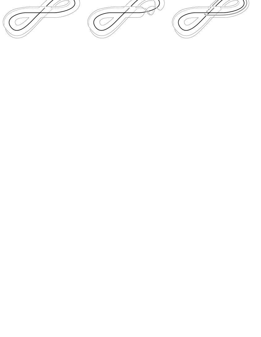
Figure 14: The abalone, and a ${\rm C}^{1}$ knot on it.

abalone, a branched standard spine of $S^{3}$, which we denote by $A$. Note that $A$ has one vertex, two edges and two regions. The figure on the left is easier to understand, but it does not represent the genuine embedding of $A$ in $S^{3}$, which is instead shown in the centre (hint: compute linking numbers). On the right we show (using the easier picture) a ${\rm C}^{1}$ knot $K$ on $A$. Using the genuine picture one sees that $K$ is actually trivial in $S^{3}$, and its framing is $-1$. So the knot complement $E(K)$ is actually a solid torus, with an induced Euler structure $\xi$, and the white annulus $W\subset\partial E(K)$ is a longitudinal one. Let us now take the representation $\varphi:\pi_{1}(E(K))\to{\hbox{\Bbb Z}}[t^{\pm 1}]$ which maps the generator to $t$. It is not hard to see that $H_{*}^{\varphi}(E(K),\overline{W})=0$, so we can compute $\tau^{\varphi}(E(K),\xi)$. We describe the method to be followed, skipping several details and all explicit formulae.

We can apply directly the method described in the (partial) proof of Theorem 4.3, to get a branched standard spine $P$ (in the sense of Theorem 4.3) of $E(K)$. This $P$ is easily recognized to have 5 vertices (denoted $v_{1},\dots,v_{5}$), 10 edges (denoted $e_{0},\dots,e_{9}$) and 6 regions (denoted $r_{1},\dots r_{6}$). Figure 15 shows the truncated ideal triangulation dual to $P$.

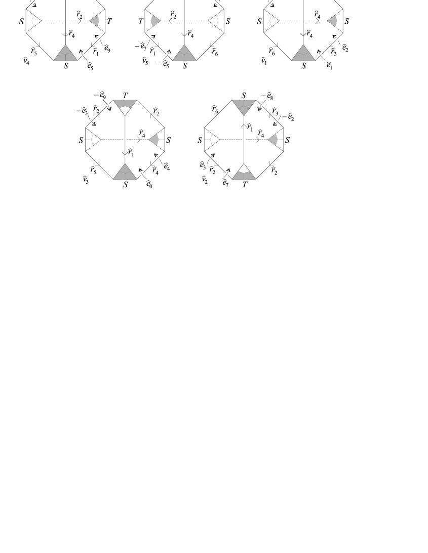
Figure 15: Truncated ideal triangulation of the knot complement.

In the figure the hat denotes duality as usual. We have written $-\hat{e}_{i}$ instead of $\hat{e}_{i}$ when $\hat{e}_{i}$ lies on $\hat{v}_{j}$ but the natural orientation of $\hat{e}_{i}$ is not induced by the orientation of $\hat{v}_{j}$. The letters $S$ and $T$ refer to the boundary sphere and torus respectively ($S$ should actually be collapsed to one point $x_{0}$, but the picture is easier to understand before collapse).

Recall that the algebraic complex of which we must compute the torsion has one generator for each cell in the cellularization of $E(K)$ arising from $P$, excluding the white cells and the tangency circles on the boundary. From Fig. 15 we can see how many such cells there will be in each dimension, namely 3 in dimension 0 ($x_{0}$ and two vertices on $T$), 14 in dimension 1 (the $\hat{r}_{i}$’s and 8 edges on $T$), 16 in dimension 2 (the $\hat{e}_{i}$’s and the 6 black kites on $T$) and 5 in dimension 3 (the $\hat{v}_{i}$’s). We can also easily describe the combinatorial Euler chain $s^{\prime}(P)$ which will be used to find the preferred cell liftings: besides the orbits of the field there are only one star and one bi-arrow; the support of $s^{\prime}(P)$ has 3 connected components (one spider with 19 legs and head at $x_{0}$, the star union the second half of $\hat{r}_{2}$, and the bi-arrow union a segment contained in $\hat{e}_{3}$).

To actually determine the preferred liftings we need an effective description of the lifting of the cellularization to the universal cover $\tilde{E}(K)\to E(K)$. Since $\pi_{1}(E(K))={\hbox{\Bbb Z}}$, each cell $c$ will have liftings $\tilde{c}^{(n)}$ for $n\in{\hbox{\Bbb Z}}$, where $\tilde{c}^{(n)}$ is the $n$-th translate of $\tilde{c}^{(0)}$. The choice of $\tilde{c}^{(0)}$ itself is of course arbitrary, but to understand the cover we must express the $\partial\tilde{c}^{(0)}$’s in terms of the other $\tilde{d}^{(n)}$’s. To do this we start with a lifting $\tilde{x}_{0}$ of the basepoint $x_{0}$ and we lift the other cells one after each other, taking into account the relations in $\pi_{1}(E(K)$ and making sure that the union of cells already lifted is always connected. When a cell $c$ is reached for the first time, its lifting is chosen arbitrarily and declared to be $\tilde{c}^{(0)}$, but its boundary will involve in general $\tilde{d}^{(n)}$’s with $n\neq 0$. Once the lifted cellularization is known, it is a simple matter to determine preferred cell liftings: since the support of $s^{\prime}(P)$ consists of 3 spiders, we only need to choose liftings of the 3 heads and then lift the legs.

Carrying out the computations we have explicitly found the algebraic complex with coefficients in ${\hbox{\Bbb Z}}[t^{\pm 1}]$, and the preferred generators of the 4 moduli appearing. Then, using Maple, we have checked that indeed the complex is acyclic, and we have computed its torsion as follows:

$$\tau^{\varphi}(E(K),\xi)=\pm t^{-1}.$$

Note that as an application of Proposition 2.17, by adding curls, we can easily construct a family $\{K_{n}\}$ of pseudo-Legendrian knots such that $\tau^{\varphi}(E(K_{n}),\xi_{n})=\pm t^{n}$.

6 Main proofs

In this section we provide all the proofs which we have omitted in the rest of the paper. We will always refer to the statements for the notation.

Proof of  1.1. Let us first recall the classical Poincaré-Hopf formula, according to which if $v$ is a vector field with isolated singularities on a manifold $M$, and $v$ points outwards on $\partial M$ (i.e. $\partial M$ is black), then the sum of the indices of all singularities is $\chi(M)$. Assume now that $v$ has isolated singularities and on $\partial M$ it is compatible with a pattern ${\cal P}=(W,B,V,C)$. We claim that if ${\cal C}$ is a cellularization of $M$ suited to ${\cal P}$ we have:

$$\sum_{x\in{\rm Sing}(v)}{\rm ind}_{x}(v)=\chi(M)-\sum_{\sigma\in{\cal C},\ \sigma\subset W\cup V}{\rm ind}(\sigma).$$ (6)

This formula is enough to prove the statement: if a non-singular field $v$ compatible with ${\cal P}$ exists then the left-hand side of 6 vanishes, and the right-hand side of 6 equals the obstruction of the statement. On the other hand, if the obstruction vanishes, then one can first consider a singular field compatible with ${\cal P}$, then group up the singularities in a ball, and remove them.

To prove 6 we consider the manifold $M^{\prime}$ obtained by attaching a collar $\partial M\times[0,1]$ to $M$ along $\partial M=\partial M\times\{0\}$. Of course $M^{\prime}\cong M$. We will now extend $v$ to a field $v^{\prime}$ on $M^{\prime}$ with the property that $v^{\prime}$ points outwards on $\partial M^{\prime}$, and in $\partial M\times(0,1)$ the field $v^{\prime}$ has exactly one singularity for each cell $\sigma\subset W\cup V$, with index ${\rm ind}(\sigma)$. An application of the classical Poincaré-Hopf formula then implies the conclusion. The construction of $v^{\prime}$ is done cell by cell. We first show how the construction goes in dimension 2, see Fig. 16.

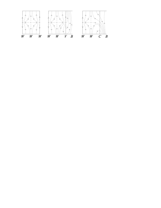
Figure 16: Extension of a field to the collared manifold: dimension 2

For the 3-dimensional case, it is actually convenient to choose a cellularization ${\cal C}$ of special type. Namely, we assume that ${\cal C}\big{|}_{\partial M}$ consists of rectangles and triangles, each rectangle having exactly one edge on $V\cup C$, and the union of rectangles covering a neighbourhood of $V\cup C$. We suggest in Fig. 17 how to

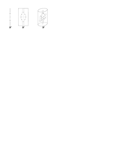
Figure 17: Extension of a field to the collared manifold: white cells in dimension 3

define $v^{\prime}$ on $\sigma\times[0,1]$ for $\sigma\subset W$ of dimension 0, 1 and 2 respectively. By the choices we have made the situation near $\partial W$ contains the 2-dimensional situation as a transversal cross-section, and it is not too difficult to extend $v^{\prime}$ further and check that indices of the singularities are as required. As an example, we suggest in Fig. 18

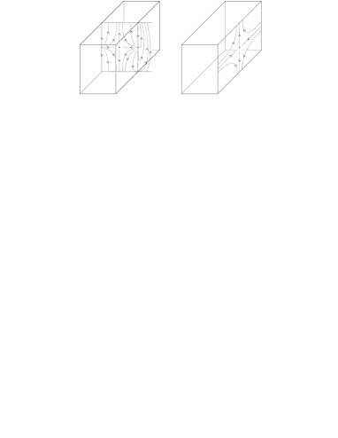
Figure 18: Extension of a field to the collared manifold: convex edge in dimension 3

how to do this near a convex edge.  1.1

Proof of  1.5. Our proof follows the scheme given by Turaev in [27], with some technical simplifications and some extra difficulties due to the tangency circles. We first recall that if ${\cal S}$ is a (smooth) triangulation of a manifold $N$, a (singular) vector field $w_{\cal S}$ on $N$ can be defined by the requirements that: (1) each simplex is a union of orbits; (2) the singularities are exactly the barycentres of the simplices; (3) barycentres of higher dimensional simplices are more attractive that those of lower dimensional simplices. More precisely, each orbit (asymptotically) goes from a barycentre $p_{\sigma}$ to a barycentre $p_{\sigma^{\prime}}$, where $\sigma\subset\sigma^{\prime}$. It is automatic that ${\rm ind}_{p_{\sigma}}(w_{\cal S})={\rm ind}(\sigma)$. See Fig. 19 for a description of $w_{\cal S}$ on a 2-simplex of ${\cal S}$.

Figure 19: The singular field $w_{\cal S}$ on a 2-simplex

Let us consider now a triangulation ${\cal T}$ of $M$, and let us choose a representative $z$ of the given $\xi\in{\rm Eul}^{\rm c}(M,{\cal P})$ as in Proposition 1.4(3). We consider now the manifold $M$ obtained by attaching $\partial M\times[0,\infty)$ to $M$ along $\partial M=\partial M\times\{0\}$. Note that $M^{\prime}\cong{\rm Int}(M)$. Moreover ${\cal T}$ extends to a “triangulation” ${\cal T}^{\prime}$ of $M^{\prime}$, where on $M\times(0,\infty)$ we have simplices with exactly one ideal vertex, obtained by taking cones over the simplices in $\partial M$ and then removing the vertex. Even if ${\cal T}^{\prime}$ is not strictly speaking a triangulation, the construction of $w_{{\cal T}^{\prime}}$ makes sense, because the missing vertex at infinity would be a repulsive singularity anyway. We arrange things in such a way that if $\sigma\subset\partial M$ then the singularity in $\sigma\times(0,\infty)$ is at height $1$, so it is $p_{\sigma}\times\{1\}$.

We will define now a smooth function $h:\partial M\to(0,\infty)$ and set $M_{h}=M\cup\{(x,t)\in\partial M\times[0,\infty):\ t\leq h(x)\}$, in such a way that $w_{{\cal T}^{\prime}}$ is non-singular on $\partial M_{h}$, and, modulo the natural homeomorphism $M\cong M_{h}$, it induces on $\partial M_{h}$ the desired boundary pattern ${\cal P}$. Later we will show how to use $z$ to remove the singularities of $w_{{\cal T}^{\prime}}$ on $M_{h}$.

To define the function $h$ we consider a (very thin) left half-collar $L$ of $V$ on $\partial M$ and a right half-collar $R$ of $C$. Here “left” and “right” refer to the natural orientations of $\partial M$ and of $V\cup C$. Note that $L\subset B$ and $R\subset W$. Now we set $h\big{|}_{B\setminus L}\equiv 1/2$, and $h\big{|}_{W\setminus R}\equiv 2$. Figures 20 and 21

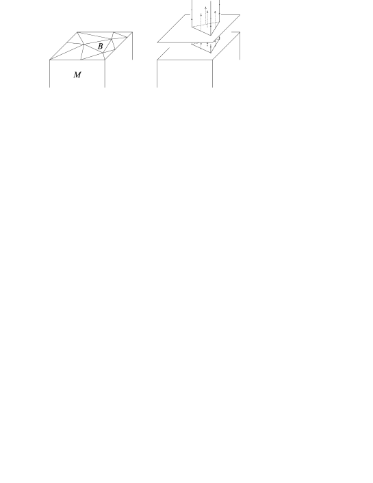
Figure 20: Where $h=1/2$ the field points outwards

respectively show that away from $V\cup C$ indeed the pattern of $w_{{\cal T}^{\prime}}$ on

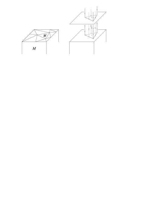
Figure 21: Where $h=2$ the field points inwards

$\partial M_{h}$ is as required. Now we identify $L$ to $V\times[-1,0]$ and $R$ to $C\times[0,1]$, and we define $h(x,s)=f(s)$ for $(x,s)\in V\times[-1,0]$ and $h(x,s)=f(s-1)$ for $(x,s)\in C\times[0,1]$, where $f:[-1,0]\to[1/2,2]$ is a smooth monotonic function with all the derivatives vanishing at $-1$ and $0$. Instead of describing $f$ explicitly we picture it and show that also near $V\cup C$ the pattern is as required. This is done near $V$ and $C$ respectively in Figg. 22

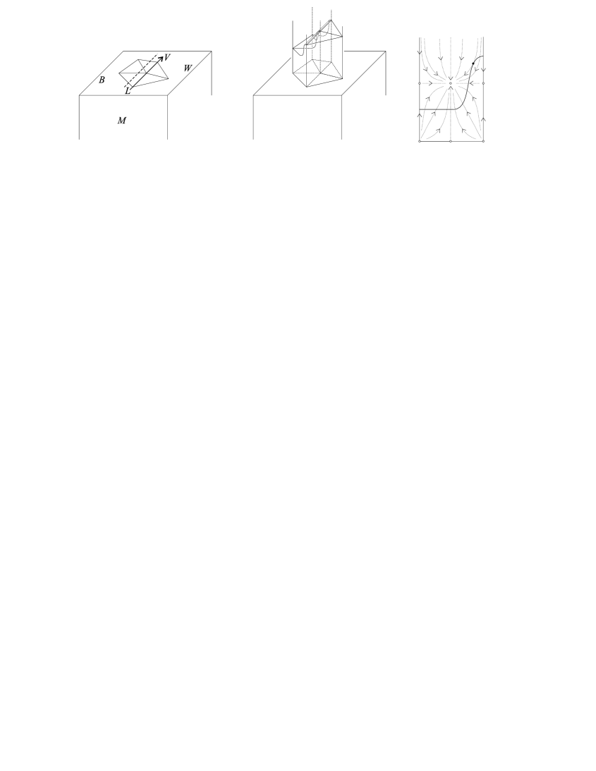
Figure 22: On $V$ the field has convex tangency

and 23.

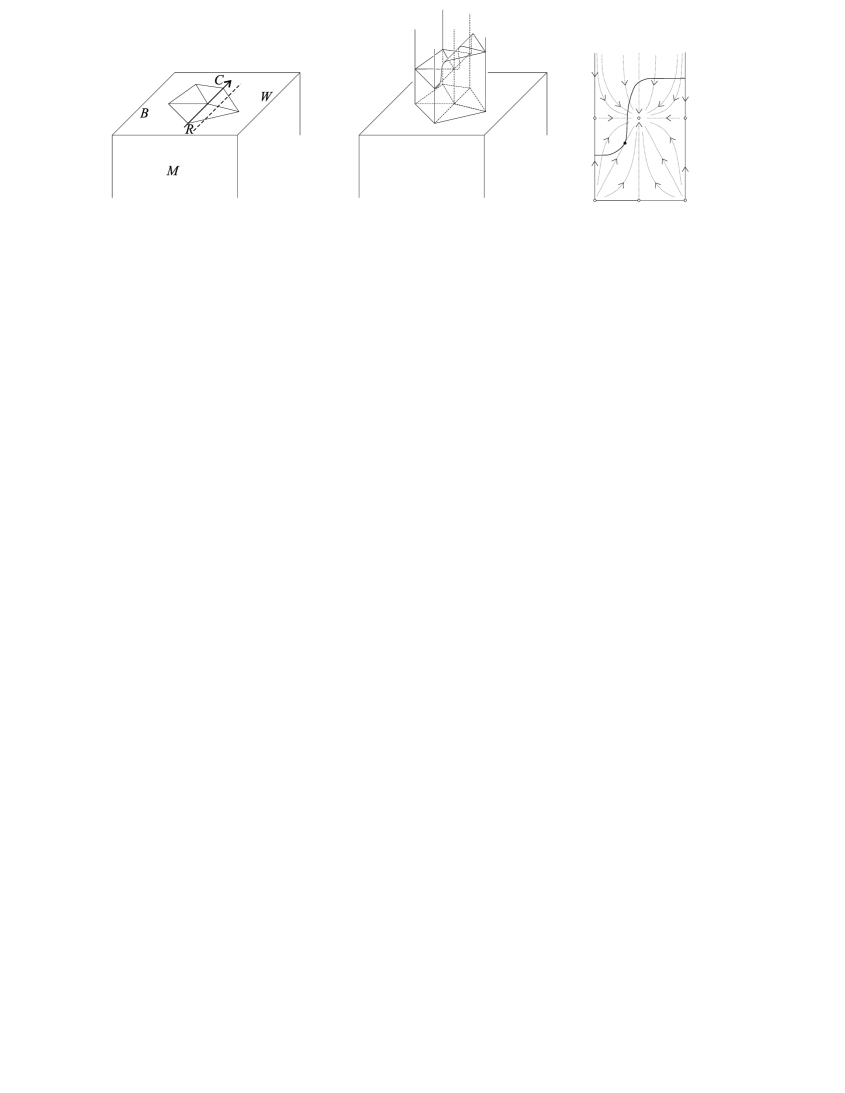
Figure 23: On $C$ the field has concave tangency

In both pictures we have only considered a special configuration for the triangulation on $\partial M$, and we have refrained from picturing the orbits of the field in the 3-dimensional figure. Instead, we have separately shown the orbits on the vertical simplices on which the value of $h$ changes.

The conclusion is now exactly as in Turaev’s argument, so we only give a sketch. The chosen representative $z$ of $\xi\in{\rm Eul}^{\rm c}(M,{\cal P})$ can be described as an integer linear combination of orbits of $w_{{\cal T}^{\prime}}$, which we can describe as segments $[p_{\sigma},p_{\sigma^{\prime}}]$ with $\sigma\subset\sigma^{\prime}$. Now we consider the chain

$$z^{\prime}=z-\sum_{\sigma\subset W\cup V}{\rm ind}(\sigma)\cdot p_{\sigma}\times[0,1].$$ (7)

By definition of $h$ we have that $z^{\prime}$ is a 1-chain in $M_{h}$, and $\partial z^{\prime}$ consists exactly of the singularities of $w_{{\cal T}^{\prime}}$ contained in $M_{h}$, each with its index. For each segment $s$ which appear in $z^{\prime}$ we first modify $w_{{\cal T}^{\prime}}$ to a field which is “constant” on a tube $T$ around $s$, and then we modify the field again within $T$, in a way which depends on the coefficient of $s$ in $z^{\prime}$. The resulting field has the same singularities as $w_{{\cal T}^{\prime}}$, but one checks that these singularities can be removed by a further modification supported within small balls centred at the singular points. We define $\Psi(\xi)$ to be the class in ${\rm Eul}^{\rm s}(M,{\cal P})$ of this final field. Turaev’s proof that $\Psi$ is indeed well-defined and $H_{1}(M;{\hbox{\Bbb Z}})$-equivariant applies without essential modifications.  1.5

Remark 6.1

In the previous proof we have defined $\Psi$ using triangulations, in order to apply directly Turaev’s technical results (in particular, invariance under subdivision). However the geometric construction makes sense also for cellularizations ${\cal C}$ more general than triangulations, the key point being the possibility of defining a field $w_{{\cal C}}$ satisfying the same properties as the field defined for triangulations. This is certainly true, for instance, for cellularizations ${\cal C}$ of $M$ induced by realizations of $M$ by face-pairings on a finite number of polyhedra, assuming that the projection of each polyhedron to $M$ is smooth.

Proof of  1.9. To help the reader follow the details, we first outline the scheme of the proof:

1. By identifying $M$ to a collared copy of itself, we choose a representative $z$ of the given $\xi\in{\rm Eul}^{\rm c}(M,{\cal P})$ such that the extra terms added to define $\Theta^{\rm c}(\xi)$ cancel with terms already appearing in $z$. (We know a priori that this happens at the level of boundaries, but it may well not happen at the level of $1$-chains.)

2. We apply Remark 6.1 and choose a cellularization of $M$ in which it is particularly easy to analyze $\Psi(\xi)$ and $\Psi(\Theta^{\rm c}(\xi))$, both constructed using the representative $z$ already obtained.

We consider a cellularization ${\cal C}$ of $M$ satisfying the same assumptions on $\partial M$ as those considered in the proof of Proposition 1.1, namely $C\cup V$ is surrounded on both sides by a row of rectangular tiles, and the other tiles are triangular. We denote by $\gamma_{1},\dots,\gamma_{n}$ the segments in $C$, oriented as $C$.

Let us consider a representative $z$ relative to ${\cal C}$ of the given $\xi\in{\rm Eul}^{\rm c}(M,{\cal P})$. We construct a new copy $M_{1}$ of $M$ by attaching $\partial M\times[-1,0]$ to $M$ along $\partial M=\partial M\times\{-1\}$, and we extend ${\cal C}$ to ${\cal C}_{1}$ by taking the product cellularization on $\partial M\times[-1,0]$. We define a new chain as

$$z_{1} = z+\sum_{\sigma\subset B}{\rm ind}(\sigma)\cdot p_{\sigma}\times[-1/2,0]-\sum_{\sigma\subset W\cup V}{\rm ind}(\sigma)\cdot p_{\sigma}\times[-1,-1/2]$$

$$+\sum_{j=1}^{n}\Big{(}\gamma_{j}\big{|}_{[1/2,1]}\times\{-1/2\}-\gamma_{j}\big{|}_{[1/2,1]}\times\{0\}\Big{)}.$$

Note that $z_{1}$ is an Euler chain in $M_{1}$ with respect to ${\cal C}_{1}$. Consider the natural homeomorphism $f:M\to M_{1}$ and the class

$$a=\alpha^{\rm c}(f_{*}(\xi),[z_{1}])\in H_{1}(M_{1};{\hbox{\Bbb Z}})$$

which may or not be zero. Since the inclusion of $M$ into $M_{1}$ is an isomorphism at the $H_{1}$-level, $a$ can be represented by a $1$-chain in $M$, so $z_{1}$ can be replaced by a new Euler chain $z_{2}$ such that $[z_{2}]=f_{*}(\xi)$ and $z_{2}$ differs from $z_{1}$ only on $M$.

Renaming $M_{1}$ by $M$ and $z_{2}$ by $z$ we have found a representative $z$ of $\xi$ such that $z=z_{\theta}+\sum_{j=1}^{n}\gamma_{j}\big{|}_{[1/2,1]}$, where $z_{\theta}$ is a sum of simplices contained in $B\cup{\rm Int}M$. Note that of course $\Theta^{\rm c}(\xi)=[z_{\theta}]$. To conclude the proof we need now to analyze $\Psi(\xi)$, constructed using $z$, and $\Psi(\Theta^{\rm c}(\xi))$, constructed using $[z_{\theta}]$, and show that $\Psi(\Theta^{\rm c}(\xi))=\Theta^{\rm s}(\Psi(\xi))$. By construction $\Psi(\xi)$ and $\Psi(\Theta^{\rm c}(\xi))$ will only differ near $C$, and we concentrate on one component of $C$ to show that the difference is exactly (up to homotopy) as in the definition of $\Theta^{\rm s}$, i.e. as in Fig. 3.

The difference between $\Psi(\xi)$ and $\Psi(\Theta^{\rm c}(\xi))$ is best visualized on a cross-section of the form $C\times[0,\infty)$. We leave to the reader to analyze the complete 3-dimensional pictures. To understand the cross-section, we follow the various steps in the proof of Theorem 1.5.

The first step in the definition of $\Psi(\xi)$ (respectively, $\Psi(\Theta^{\rm c}(\xi))$) consists in choosing the height function $h$ (respectively, $h_{\theta}$) and replacing the chains $z$ (respectively, $z_{\theta}$) by a chain $z^{\prime}$ (respectively, $z^{\prime}_{\theta}$) as in formula (7). This is done in Fig. 24

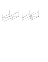
Figure 24: Local difference between $z^{\prime}$ (left) and $z^{\prime}_{\theta}$ (right)

where only the difference between the chains is shown.

To conclude we must modify the field $w_{\cal C}$ within a small neighbourhood of the support of $z^{\prime}$ and $z^{\prime}_{\theta}$. This is done in Figg. 25

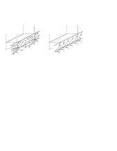
Figure 25: Construction of $\Psi(\xi)$ on $C\times[0,\infty)$. On the left we show $w_{\cal C}$ and the zones where it must be modified.

and 26 respectively. The rightmost picture in Fig. 26

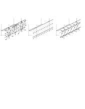
Figure 26: Construction of $\Psi(\Theta^{\rm c}(\xi))$ on $C\times[0,\infty)$

is obtained by homotopy on the previous one. The representatives of $\Psi(\xi)$ and $\Psi(\Theta^{\rm c}(\xi))$ can be compared directly, and indeed they differ by a curve parallel to $C$ and directed consistently with $C$, so $\Psi(\Theta^{\rm c}(\xi))=\Theta^{\rm s}(\Psi(\xi))$.  1.9

We give now the proof omitted in Section 2.

Proof of  2.17. Let us first note that the comparison class which we must show to be $[m]$ is independent of $f$ by Proposition 2.8. We will give two completely independent (but somewhat sketchy) proofs that this class is indeed $[m]$.

For a first proof, instead of comparing a “straight” knot with one with two curls, we compare two knots with one curl, chosen so that the framing is the same but the winding number is different. This is of course equivalent. The two knots are shown in Fig. 27 as thick tubes, together with one specific orbit of the field they are immersed in. The resulting bicoloration on the boundary of the tubes is also outlined.

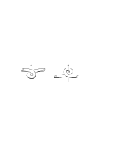
Figure 27: Differently curled tubes in the vertical field.

To compare the curls we isotope the bicolorated tubes to the same straight tube, and we show how the orbit of the field is transformed under this isotopy. This is done in Fig. 28.

Figure 28: Straightened curls.

Also from this very partial picture it is quite evident that the resulting fields wind in opposite directions around the tube. A more accurate picture would show that the difference is actually a meridian of the tube.

Another (indirect) proof goes as follows. Note first that the comparison class which we must compute certainly is a multiple of $[m]$, say $k\cdot[m]$. Note also that $k$ is independent of the ambient manifold $(M,v)$. Moreover, by symmetry, we will have $\alpha(\xi(v,K_{0}),f_{*}(\xi(v,K_{-1})))=-k\cdot[m]$ if $K_{-1}$ is obtained by locally adding a double curl with opposite winding number.

We take now $M$ to be $S^{3}$, with the field $v$ carried by the abalone $P$ as in Section 5, and $K$ to be a trivial knot contained in the “smaller” disc of the $P$. We apply Proposition 2.13 to find another pseudo-Legendrian knot $K^{\prime}$ in $(S^{3},v)$ such that $\alpha(\xi(v,K),\xi(v,K^{\prime}))=[m]$, where by simplicity we are omitting the framed-isotopies necessary to compare these classes. As already remarked in Section 4, we can assume that $K^{\prime}$ has a ${\rm C}^{1}$-projection on $P$. If one examines $P$ carefully one easily sees that $K^{\prime}$ can actually be slid over $P$ to lie again in the small disc of $P$. Now $K^{\prime}$ is a planar projection of the trivial knot, so through Reidemeister moves of types II and III, which correspond to isotopies throgh knots transversal to $v$, it can be transformed into a projection which differs from the trivial one only for a finite (even) number of curls. Summing up, we have a knot $K^{\prime}$ such that $\alpha(\xi(v,K),\xi(v,K^{\prime}))=[m]$ and $K^{\prime}$ differs from $K$ only for a finite number of transformations of the form $K\mapsto K_{1}$ or $K\mapsto K_{-1}$. This shows that $[m]$ is a multiple of $k\cdot[m]$, so $k=\pm 1$.  2.17

We conclude the paper by establishing the only statement given in Section 4 and not proved there. As above, we do not recall all the notation.

Proof of  4.9. We fix $P$ and set $s^{\prime\prime}=s^{\prime\prime}(P)$, ${\widehat{v}}={\widehat{v}}(P)$. Using Remark 6.1 we see that the construction of $\Psi([s^{\prime\prime}])$ explained in the proof of Theorem 1.5 can be directly applied to the cellularization ${\widehat{{\cal T}}}={\widehat{{\cal T}}}(P)$ of ${\widehat{M}}$. Recall that this construction requires identifying ${\widehat{M}}$ to a collared copy of itself, and extending $s^{\prime\prime}$ to a chain $s^{\prime\prime\prime}$ whose boundary consists precisely of the singularities of a field $w$. A representative of $\Psi([s^{\prime\prime}])$ is then obtained by applying to $w$ a certain desingularization procedure. This desingularization is supported in a neighborhood of $s^{\prime\prime\prime}$, and one can easily check that the connected components of the support of $s^{\prime\prime\prime}$ (denoted henceforth by $S$) are actually contractible. Therefore, any desingularization of $w$ supported in a neighbourhood of $s^{\prime\prime\prime}$ will give a representative of ${\widehat{v}}$. We will prove the desired formula $\Psi([s^{\prime\prime}])=[{\widehat{v}}]$ by exhibiting one such desingularization which is nowhere antipodal to ${\widehat{v}}$. In our argument we will always neglect the contraction of $S^{2}_{\rm triv}$ which maps $M$ onto ${\widehat{M}}$. (The desired formula actually holds at the level of $M$, and it easily implies the formula for ${\widehat{M}}$.)

By the above observations, the following claims easily imply the conclusion of the proof:

1. The set of points where $w$ is antipodal to ${\widehat{v}}$ is contained in $S$.

2. If $S_{0}$ is a component of $S$ then $w$ can be desingularized within a neighbourhood of $S_{0}$ to a field which is not antipodal to ${\widehat{v}}$ in the neighbourhood.

We prove claim 1 by first noting that the cells dual to those of $P$ are unions of orbits of both $w$ and ${\widehat{v}}$. So we can analyze cells separately. We do this explicitly only for 2-dimensional cells, leaving to the reader the other cases. In Fig. 29

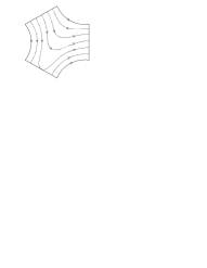
Figure 29: The field ${\widehat{v}}$ on a hexagon

we describe ${\widehat{v}}$. In the left-hand side of Fig. 30

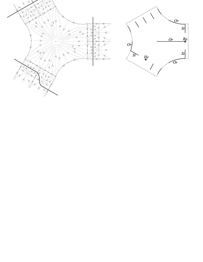
Figure 30: The field $w$ and the trace of $S$ on a hexagon

we describe $w$ on the collared hexagon. In the right-hand side of the same figure we only show the singularities of $w$ on the renormalized hexagon, and the intersection of $S$ with the hexagon. In this figure the 7 short segments come from $s^{\prime\prime\prime}-s^{\prime\prime}$; the other bits of $S$ have been labeled by ‘Or’, ‘St’, ‘Ba’ or ‘He’ to indicate that they come from orbits of ${\widehat{v}}$, stars, bi-arrows or half-edges.

This proves claim 1. Comparing Fig. 30 with Fig. 29, and carrying out the same analysis for 3-cells, one actually shows also claim 2 for components $S_{0}$ coming from $s^{\prime\prime\prime}-s^{\prime\prime}$. Components of $S$ other than these can be described in one of the following ways:

• an orbit of ${\widehat{v}}$ emanating from a vertex of $P$;

• a half-edge of $C$;

• a bi-arrow together with an orbit of ${\widehat{v}}$ emanating from the centre of an edge of $P$ and reaching the centre of the bi-arrow;

• a star together with an orbit of ${\widehat{v}}$ emanating from the centre of a disc of $P$ and reaching the centre of the star.

All cases can be treated with the same method, we only do case (c). Figure 31

Figure 31: An enhanced bi-arrow and the field $w$ near it

shows the component placed so that ${\widehat{v}}$ can be thought of as the constant vertical field pointing upwards, and the field $w$ near the component. The conclusion easily follows.  4.9

benedett@dm.unipi.it

petronio@dm.unipi.it

Dipartimento di Matematica

Via F. Buonarroti, 2

I-56127, PISA (Italy)

References

- [1] R. Benedetti, C. Petronio, A finite graphic calculus for -manifolds, Manuscripta Math. 88 (1995), 291-310.
- [2] R. Benedetti, C. Petronio, “Branched Standard Spines of 3-Manifolds”, Lecture Notes in Math. n. 1653, Springer-Verlag, Berlin-Heidelberg-New York, 1997.
- [3] R. Benedetti, C. Petronio, Branched spines and contact structures on -manifolds, Ann. Mat. Pura Appl. (to appear).
- [4] R. Benedetti, C. Petronio, Combings on -manifolds with boundary: combinatorial encoding and Reidemeister torsion, (in preparation).
- [5] R. Benedetti, C. Petronio, Euler structures with generic boundary and torsion of Reidemeister type, (in preparation).
- [6] D. Bennequin, Entrelacements et équations de Pfaff, Astérisque 107-108 (1983).
- [7] B. G. Casler, An imbedding theorem for connected -manifolds with boundary, Proc. Amer. Math. Soc. 16 (1965), 559-566.
- [8] J. Christy, Branched surfaces and attractors I, Trans. Amer. Math. Soc. 336 (1993), 759-784.
- [9] Ya. Eliashberg, Classification of overtwisted contact structures, Invent. Math. 98 (1989), 623-637.
- [10] R. Fintushel, R. Stern, Knots, links, and -manifolds, Invent. Math. 134 (1998), 363-400.
- [11] D. Gillman, D. Rolfsen, The Zeeman conjecture is equivalent to the Poincaré conjecture, Topology 22 (1983), 315-323.
- [12] A. Hatcher, D. McCullough, Finiteness of classifying spaces of relative diffeomorphism groups of -manifolds, Geometry and Topology 1 (1997), 91-109.
- [13] I. Ishii, Moves for flow-spines and topological invariants of -manifolds, Tokyo J. Math. 15 (1992), 297-312.
- [14] T. T. Q. Le, J. Murakami, T. Ohtsuki, On a universal perturbative invariant of -manifolds, Topology 37 (1998), 359-374.
- [15] C. Lescop,“Global Surgery Formula for the Casson-Walker invariant”, Ann. of Math. Studies n. 140, Princeton University Press, Princeton, NJ, 1996.
- [16] C. Lescop, A sum formula for the Casson-Walker invariant, Invent. Math. 133 (1998), 613-681.
- [17] S. V. Matveev, A. T. Fomenko, Constant energy surfaces of Hamiltonian systems, enumeration of three-dimensional manifolds in increasing order of complexity, and computation of volumes of closed hyperbolic manifolds, Russ. Math. Surv. 43 (1988), 3-25.
- [18] S. V. Matveev, Transformations of special spines and the Zeeman conjecture, Math. USSR-Izv. 31 (1988), 423-434.
- [19] S. V. Matveev, “Algorithmic Methods in 3-Manifold Topology”, in preparation.
- [20] G. Meng, C. H. Taubes, Milnor torsion, Math. Res. Lett. 3 (1996), 661-674
- [21] J. Milnor, Whitehead torsion, Bull. Amer. Math. Soc 72 (1966), 358-426.
- [22] C. Petronio, “Standard Spines and 3-Manifolds”, Scuola Normale Superiore, Pisa, 1995.
- [23] R. Piergallini, Standard moves for standard polyhedra and spines, Rendiconti Circ. Mat. Palermo 37, suppl. 18 (1988), 391-414.
- [24] J. Porti, “Torsion de Reidemeister pour les Variétés Hyperboliques”, Memoirs n. 612, Amer. Math. Soc., Providence, RI, 1997.
- [25] B. Trace, On the Reidemeister moves of a classical knot, Proc. Amer. Math. Soc. 89 (1983), 722-724.
- [26] V. G. Turaev, Reidemeister torsion in knot theory, Russ. Math. Surv. 41 (1986), 119-182.
- [27] V. G. Turaev, Euler structures, nonsingular vector fields, and torsion of Reidemeister type, Math. USSR-Izv. 34 (1990), 627-662.
- [28] V. G. Turaev, Torsion invariants of Spinc-structures on -manifolds, Math. Res. Lett. 4 (1997), 679-695.
- [29] V. G. Turaev, A combinatorial formulation for Seiberg-Witten invariants of -manifolds, Math. Res. Lett. 5 (1998), 583-598.