Area preservation in computational fluid dynamics

Abstract

Incompressible two-dimensional flows such as the advection (Liouville) equation and the Euler equations have a large family of conservation laws related to conservation of area. We present two Eulerian numerical methods which preserve a discrete analog of area. The first is a fully discrete model based on a rearrangement of cells; the second is more conventional, but still preserves the area within each contour of the vorticity field. Initial tests indicate that both methods suppress the formation of spurious oscillations in the field.

1 Introduction

When a smooth field $\omega(x,y)$ is advected by an area-preserving flow, the area within each contour of $\omega$ is preserved. This is seen in pure advection and in the Euler equations, for example, and is important in the numerical solution of two-phase free boundary problems, where the total volume of each fluid should be preserved. Yet, although the advection problem has been addressed in probably thousands of papers, and very accurate, stable, and efficient methods are known, no existing numerical methods take the area-preservation property into account. In this Letter we present an initial study containing two methods which do preserve (a discrete analog of) area. Although they are not, presumably, competitive with the best existing methods for advection, the results are extremely promising.

The configuration space of an inviscid incompressible fluid is the group ${\cal D}_{\mu}$ of volume-preserving diffeomorphisms of the fluid’s domain; the ‘Arnold’ picture, in which the Euler equations are geodesic equations on this group equipped with the kinetic energy ($L_{2}$) metric, is treated in [2]. The configuration at any time is a volume-preserving rearrangement of the initial condition. Existing Eulerian numerical methods do not preserve any discrete analogue of this property. This is particularly relevant in two dimensions, where area preservation leads to an infinite number of conserved quantities, the generalized enstrophies.

We consider a two-dimensional fluid with divergence-free velocity field ${\bf u}=(u,v)$, stream function $\psi$ (i.e. $u=\psi_{y}$, $v=-\psi_{x}$), and some quantity $\omega$, which we call the vorticity, which is advected by the fluid:

$$\dot{\omega}+{\bf u}\cdot\nabla\omega=\dot{\omega}+J(\omega,\psi)=0,$$ (1)

where the Jacobian

$$J(a,b)={\partial(a,b)\over\partial(x,y)}.$$ (2)

In the two situations we shall consider, this is a Hamiltonian system with Poisson bracket

$$\{F,G\}=\int\omega J(\delta F,\delta G)\,dxdy$$ (3)

and Hamiltonian

$$H={1\over 2}\int\psi\omega\,dxdy$$

where the stream function $\psi$ is either a given function $\psi=\psi(x,y,t)$, in which case Eq. (1) is the Liouville (advection) equation, or is determined by the Poisson equation $\nabla^{2}\psi=-\omega$, in which case (1) is the the two-dimensional Euler equation. Other two-dimensional flows such as the shallow water and semi-geostrophic equations also possess a quantity $\omega$, called a potential vorticity, that is advected according to Eq. (1). There are also applications to level-set methods, in which $\omega$ is not a physical variable but is introduced so that the curve $\omega(x,y)=c$ can indicate a free boundary.

The Casimirs of the Poisson bracket (3) are conserved quantities of the PDE (3). These can be variously written as

$$C_{f}=\int f(\omega)\,dxdy$$

for any function $f$ such that $C_{f}$ exists, as

$$C_{n}=\int\omega^{n}\,dxdy,$$

called the generalized enstrophies ($C_{2}$ is the usual enstrophy), or as the areas enclosed by each vorticity contour

$$A(c)=\int_{\omega\geq c}1\,dxdy.$$

They all reflect the fact that $\omega$ is being advected by an area-preserving vector field and can only reach states which are area-preserving rearrangements of its initial state. That is,

$$\omega(x,t)=\omega(\varphi_{t}^{-1}(x),0),$$

where $\varphi_{t}$ is the time-$t$ flow of the vector field ${\bf u}$.

The famous Arakawa Jacobian is an Eulerian finite difference approximation of Eq. (2) which preserves discrete analogues of the energy $H$ and the enstrophy $C_{2}$ [1, 4]. It is known to preserve the mean of the energy spectrum and to prevent some nonlinear instabilities. However, the other conserved quantities are not preserved and their role in the dynamics is not known [2].

Area preservation can also be studied in a Lagrangian framework—for example, point vortex methods could be said to be area-preserving—but Lagrangian schemes carry a lot of extra information (the particle paths) which should be decoupled from the dynamics. The dimension of the phase space is halved in Eulerian form, and further reduced by preserving (discrete analogues of) the Casimirs. For ODEs, it is well established that the best long-time results are obtained by working in the smallest possible phase space [5].

The Hamiltonian picture has been described by Marsden and Weinstein [6]. The configuration space is the group ${\cal D}_{\mu}$. The Euler equations in Lagrangian form are a canonical Hamiltonian system on $T^{*}{\cal D}_{\mu}$, and in Eulerian form are a Lie-Poisson system on the dual of the Lie algebra of ${\cal D}_{\mu}$, which is identified with the space of vorticities. The coadjoint orbits of this space are the level sets of the Casimirs, each of which is a symplectic manifold. Discretizations of the Eulerian form are not, in general, Hamiltonian systems, nor do they have conserved quantities corresponding to the Casimirs (although there is one interesting Hamiltonian discretization, the sine-Euler equations [10]).

Therefore we forget about the Hamiltonian structure and study the Casimirs—the area-preservation—and present two models in which a discrete analogue of the areas $A(c)$ is preserved. The first (Section 2), based on a literal rearrangement of cells, is interesting in that it gives a fully-discrete, cellular-automata-like model of an incompressible fluid. It does not preserve smoothness of the vorticity field (although filamentation and turbulence mean that it can’t usually stay very smooth anyway). A smooth version (Section 3) is based on computing an approximation of $A(c)$ which is smooth as a function of $c$, and relabelling the vorticity field so that $A(c)$ is constant in time. It is tested on the Liouville equation and prevents the appearance of large spurious maxima and minima in the vorticity field during its evolution.

2 The cell rearrangement model

Both of the models presented here are projection schemes. The vorticity is evolved by any sensible scheme for some short time $t$ (e.g., 1–10 time steps), and then projected onto some space of rearrangements of the original vorticity.

In this section we consider the vorticity field to be piecewise constant on a set of fixed cells, which for convenience we take to be squares with side $h$. A (minuscule!) subset of the rearrangements of the initial condition is given by the permutations of the cells. However, these can be naturally associated with the fluid flow. For, consider the area-preserving map $\varphi$ which is the time-$t$ flow of the fluid. According to a theorem of Lax [3], there is a mapping $P$ which permutes cells and which satisfies

1. $P(C)\cap\varphi(C)\neq\emptyset$ for all cells $C$; and

2. $\|P(x)-\varphi(x)\|\leq\sup_{y,z\in C}\|\varphi(y)-\varphi(z)\|+\sqrt{2}h\quad\forall x\in C.$

The dynamics of such lattice maps are often studied. For example, if the continuous map $\varphi$ is iterated on a computer, it will not be exactly a bijection or exactly area-preserving, due to round-off error. By replacing it with a lattice map and examining the limit $h\to 0$ the effects of roundoff error can be studied.

The easiest way to construct lattice maps is as a composition of shears $x_{i}^{\prime}=x_{i}$ for $i=1,\dots,d$, $x_{j}^{\prime}=\lfloor f_{j}(x_{1},\dots,x_{d})\rfloor$ for $j=d+1,\dots,n$, where $\lfloor x\rfloor$ is the nearest lattice point to $x$. This would be suitable, for example, if $\varphi$ itself were approximated by a product of shears, as is for example the flow of separable Hamiltonians $H=H_{1}(p)+H_{2}(q)$ (the flow of the Hamiltonian vector field corresponding to each $H_{i}$ is a shear). This is very fast and the permutation need not be constructed explicitly.

However, in the present case $\varphi$ can only be obtained by integrating the Lagrangian particle paths for a short time $t$, and an explicit approximating lattice map seems to be unobtainable. Scovel [8] suggested using maps of the form, e.g., $x^{\prime}=x+\lfloor J\nabla S((x+x^{\prime})/2)\rfloor$ for a suitable Poincaré generating function $S$ (here $S=(\Delta t)\psi$ would give a good approximation of the time-$\Delta t$ flow of the stream function $\psi$). However, this nonlinear, discrete equation does not seem to have solutions in general.

Thus, it seems that one must laboriously construct a table of the permutation. An algorithm which does this is described in [7]. Its running time is ${\cal O}(N^{3})$, where $N={\cal O}(1/h^{2})$ is the number of cells. One must construct lists of candidate cells (e.g., all those that intersect $\varphi(C)$) and make successive choices from these lists, backtracking when no choices remain. While practical for moderate $N$ when the dynamics of the lattice map are going to be studied intensively, in the present application $\varphi$ changes at every time step; searching for a completely new permutation every time is too expensive. This approach has been explored by Turner [9].

Luckily, there is a way out of this impasse, using the extra physical information attached to each cell: the vorticity itself. The only use of the permutation $P$ is to update the vorticity field $\omega$ by $\omega\mapsto\widetilde{\omega}$, $\widetilde{\omega}\circ P=\omega$, in order that the distribution of vorticity values remains constant. This can be achieved directly, without actually constructing a $P$ which approximates $\varphi$, by the following algorithm. Let ${\rm rank}_{t}(c)$ be the number of cells with vorticities greater than or equal to $\omega$ at time $t$, i.e.,

$${\rm rank}_{t}(c)=\#\{j:\omega(x_{j},t)\geq c\},$$

with ties broken arbitrarily to make ${\rm rank}_{t}$ an invertible function onto $\{1,\dots,N\}$. Then:

1. Update the field $\omega$ for time $t$ any standard Eulerian method; and

2. let $\widetilde{\omega}_{j}={\rm rank}_{0}^{-1}({\rm rank}_{t}(\omega_{j}))$.

The new field $\widetilde{\omega}$ can be constructed in time $N\log N$ by sorting the two lists of vorticity values at times $0$ and $t$. The largest current value is replaced by the largest original value, and so on. (Other updates, based on minimizing $\|\widetilde{\omega}-\omega\|$, are also possible.)

This algorithm can be regarded as constructing a permutation, albeit a permutation that has no relationship to the flow $\varphi$. This is a truly finite-state model of an incompressible fluid: the state space is the permutation group $S_{N}$ and the fluid dynamics reduces to the dynamics of the map $S_{N}\to S_{N}$, defined above, parameterized by the initial distribution of vorticity values. It is an almost cellular-automata-like fluid model, although lacking the local update property of CAs. It has the aesthetic appeal of capturing the vorticity-rearrangement property perfectly in a naturally discrete way, of constructing a “discrete coadjoint orbit”, and it is very cheap.

However, these advantages are offset by a practical disadvantage of lack of smoothness. The new vorticity values are selected somewhat arbitrarily from the sorted list, and the new field may be rougher than the original. This is probably unavoidable, given the chosen fully discrete state space. The noise of this imposed roughness may swamp any gains from preserving the coadjoint orbits. However, in a turbulent flow with highly filamented vorticity, the loss of smoothness may not be significant. A second consequence of the lack of smoothness is that if $|\omega(x,t)-\omega(x,0)|$ is too small, then $\widetilde{\omega}\equiv\omega$—the field cannot be updated at all. The remapping interval $t$ must be large enough to allow some change in the configuration. For example, the flow map $\varphi$ should move each cell across at least 2 cells so that the algorithm has some scope for finding a suitable permutation.

3 The vorticity relabelling model

The cell rearrangement model produces an area function $A(c)$ which is discontinuous—in fact, it is piecewise constant. To improve it, we need to

• produce a smoother approximation of $A(c)$. If $\omega(x,y)$ is a smooth function, we want an approximation of $A(c)$ which is as smooth and accurate as possible, using only the grid values $w(x_{i},y_{j})$; and

• project the vorticity function so that its area function $A(c)$ at time $t>0$ equals (or closely approximates) the initial area function.

3.1 Computing the areas enclosed by vorticity contours

We consider a compact domain $\Omega$ with area 1, usually a square or torus, on which $\omega$ is bounded with range $[\omega_{\rm min},\omega_{\rm max}]$, and of smoothness $C^{r}$. It may be degenerate, e.g., constant on open sets.

Definition 1

The area function of the field $\omega$ is the area enclosed by the set $\{(x,y):\omega(x,y)\geq c\}$, i.e.,

$$A_{\omega}:[\omega_{\rm min},\omega_{\rm max}]\to[0,1],\quad A_{\omega}(c)=\int_{\omega(x)\geq c}1\,dx\,dy$$

$A(c)$ is strictly decreasing with respect to $c$. It is $C^{r}$ at regular (noncritical) values $c$, $C^{0}$ at nondegenerate critical values, and discontinuous at $c$ if the set $\{x:\omega(x,t)=c\}$ has positive area. (Lack of differentiability at critical values can be seen by studying $\omega=-(x^{2}+y^{2})$, for which $A(c)=\pi c$ for $c\leq 0$ and $0$ for $c>0$.) Thus, its inverse $A^{-1}$ exists and is nonincreasing (i.e., more area must be enclosed by a lesser value of $\omega$.)

Let ${\cal I}$ be an interpolation or approximation operator mapping grid functions to fields, i.e. functions on $\Omega$.

Definition 2

The area function of the grid function $\omega$ is defined to be the area function of its interpolant, i.e.,

$$A_{\omega}:=A_{{\cal I}\omega}.$$

It automatically inherits the monotonicity properties of $A$. Let ${\cal R}$ be a restriction operator mapping fields to grid functions, usually by evaluating on the grid. Let $\widetilde{\omega}={\cal I}{\cal R}\omega$. The crucial observations are the following:

1. Choice of ${\cal I}$ can lead to $A_{\widetilde{\omega}}$ being as smooth as $A_{\omega}$, and of any order of accuracy as an approximation;

2. If $\widetilde{\omega}$ is piecewise linear, its contours are polygons, whose area can be found quickly for any contour topology;

3. If $\widetilde{\omega}$ has polygonal contours, $A_{\widetilde{\omega}}$ can be second order accurate and as smooth as $A_{\omega}$.

Item (1) is obvious, and is a consequence of existence of $C^{r}$ approximations to functions. An algorithm for finding the area enclosed by (unions of) polygons is given below. The most important point is (3), as it says that smooth interpolants, which are expensive in two dimensions, are not needed to compute a smooth area function.

Consider a grid function on a triangulation of $\Omega$. Interpolating by piecewise polynomials along edges only, and constructing the interpolant whose contours are line segments within each triangle (whose graph is a “ruled surface”), yields an area function which is as smooth as the interpolant at vertex (grid point) values and analytic elsewhere. Thus, only smooth one-dimensional interpolation is needed, which is relatively cheap (e.g., $C^{1}$ can be achieved using local cubics).

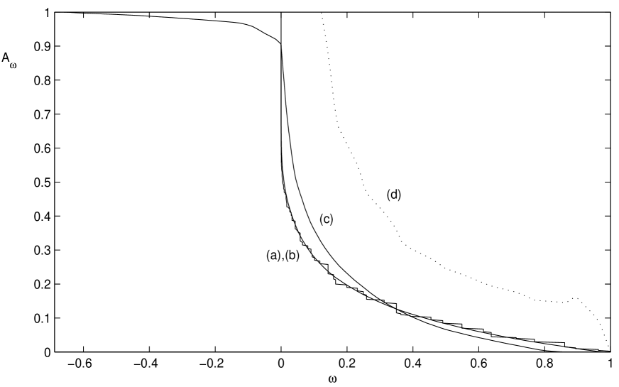
Figure 2: Numerical computation of the area enclosed within vorticity contours. (a): $C^{0}$ approximation to $A_{\omega(0)}$ using piecewise linear interpolation (Section 3). Here $\omega(0)$ is the initial condition shown in Figure 1. (b): Piecewise constant approximation to $A_{\omega(0)}$ by sorting the list of vorticity values (Section 2). (c): Area function $A_{\omega(t)}$ after evolving for time $t=1.2$ with no area preservation with an enstrophy-preserving scheme (Section 4). In the vorticity relabelling projection, vorticity values are mapped from this curve back to (a). (d): Finite difference approximation to $dA_{\omega(0)}(c)/dc$, showing that, although only $C^{0}$, for numerical purposes it can be regarded as being differentiable. The kinks in this derivative are due to $\omega$ being set to zero on the boundary.

Piecewise linear interpolation yields a $C^{0}$, second-order-accurate area function. However, it is better than its mere continuity might make it appear, since its derivative jumps at vertex values are only ${\cal O}(h^{2})$ on a grid with spacing $h$. So, numerically, it is indistinguishable from a $C^{1}$ function. In practice, the most glaring jumps are in its second derivative at vertex values, not in the function itself. (See Fig. 2.) Piecewise linear interpolation seems to be suitable in practice and this is what we use in the tests below. (If the main computational grid is square, we triangulate using an extra vertex at the center of each cell, whose value is assigned by linear interpolation.) However, true $C^{1}$ area functions have been tested as well.

The great advantage of polygonal contours is that the area of a simple polygon with vertices ${\bf x}_{i}$, $i=1,\dots,n$, is very easy to compute: it is

$${1\over 2}\sum_{i=1}^{n}{\bf x}_{i}\times{\bf x}_{i+1},$$

where $x_{n+1}:=x_{1}$. This can be seen by deriving it for a triangle, triangulating the polygon against a fixed point, and then using independence with respect to the fixed point. It can also be viewed as a discretization of

$$\int_{\Omega}1\,dx\,dy={1\over 2}\int_{\Omega}d(xdy-ydx)={1\over 2}\int_{\partial\Omega}{\bf x}\times d{\bf x}.$$

However, it would be expensive to chase contours around the domain and construct a list of simple polygons. Instead, one can simply scan each triangle for occurrence of a contour, find its endpoints ${\bf x}_{1}$, ${\bf x}_{2}$, and accumulate ${\bf x}_{1}\times{\bf x}_{2}$ with a sign determined by the sense of the triangle when its vertices are visited in order of increasing function values. This handles arbitrary contour topology. (Exception handling is needed when two vertices and the contour all have equal values.)

We are not sure if there is a similarly simple method with higher order contours. In practice, to get more than second order accuracy, we use Richardson extrapolation from a coarser grid.

For a list of contour values, the above algorithm involves scanning the cells once and accumulating areas of the relevant contours. If $N_{c}$ values of the area function are needed, and the grid size is ${\cal O}(h)$, then each cell will contain $O(hN_{c})$ contours on average, so the computation takes time ${\cal O}(N_{c}/h)$. In practice, we take $N_{c}={\cal O}(1/h)$ and build a function table, which is later interpolated as needed. Thus computing the areas takes ${\cal O}(1/h^{2})$, i.e., it is linear in the number of grid points.

If $\omega$ is nearly constant on large areas, then $A(c)$ can be very steep, so it should be tabulated using adaptive stepping in $c$. An example of the $C^{0}$ estimate of $A(c)$ given by piecewise linear interpolation is shown in Fig. 2, together with the piecewise constant estimate given by simply counting the number of vertices where $\omega>c$. Its (numerical) derivative indicates its smoothness. Some care must be taken when interpolating to maintain monotonicity.

We have also computed smooth approximations of $A_{\omega}(c)$ for random $\omega$ fields whose contours have complicated topology.

3.2 Projecting the the space of rearrangements

After evolving $\omega$ for a short time $t$ with Eulerian method, we have two grid functions, the vorticity at time $0$, $\omega(0)$, and at time $t$, $\omega(t)$. We wish to project $\omega(t)$ so that it is an (approximation of) a rearrangement of $\omega(0)$. The projection should be small and should not destroy smoothness. Traditional methods for enforcing constraints, such as steepest descents, appear to be completely infeasible because of the global and sensitive dependence of $A(c)$ on the vertex values of $\omega$. Our proposed method is a continuous version of the sorted-assignment used in the cell rearrangement model of Section 2. In words, we compute the area enclosed by the contour through each vertex value and replace it by the value that originally enclosed that much area. The contour shapes and topologies do not change: only the values associated with each contour change.

Definition 3

The relabelling projection on grid functions $\omega_{i}\approx\omega(x_{i},t)$ is defined by $\omega(t)\mapsto\widetilde{\omega}(t)$, where

$$A_{\omega(0)}(\widetilde{\omega}_{i})=A_{\omega(t)}(\omega_{i})$$ (4)

for each vertex $i$.

It is well defined by monotonicity of $A(c)$. It has an obvious continuum analog (replacing $i$ by $x$ in Eq. (4)), which if applied to every value of $\omega$ taken by a smooth vorticity field, with $\omega(0)$ and $\omega(t)$ both $C^{r}$, yields a new field $\widetilde{\omega}$ that is $C^{r}$ away from critical points of $\omega_{0}$ and $\omega_{t}$ and $C^{0}$ at such critical points.

To compute a good approximation of this projection quickly, the current area function is tabulated and interpolated at the vertex values, and then $A^{-1}_{\omega(0)}$ (which, of course, does not change during the run) is evaluated by interpolation. Of course, we do not have a true projection in that $\widetilde{\widetilde{\omega}}\neq\widetilde{\omega}$, because interpolation errors in the contours do change the contour shapes by a small amount when the vertex values are changed. We do not quite get $A_{\omega(0)}(c)=A_{\widetilde{\omega}(t)}(c)$ for all $c$. However, these errors can be controlled independently of the discretization error in $\omega$, for example, by using a higher order approximation of $A$. In a numerical test, one application of Richardson extrapolation to the areas enclosed by piecewise linear contours gave $|A_{\omega(0)}-A_{\widetilde{\omega}(t)}|\sim 10^{-4}$ on a relatively coarse $20\times 20$ grid. By contrast, without the relabelling projection, errors in the area function rapidly reach order 1.

If the vorticity is evolved for a short time $t$, with a method of spatial order $p$, spatial errors dominate the error in the area function which are ${\cal O}(th^{p})$. Thus, with $t=o(1)$, the projection only alters the field by $o(h^{p})$, and the overall method (after evolution and projection), is still consistent of the same order $p$. The projection cannot correct any errors in the shapes of the contours, but it can stop those errors growing further by propagation of the false distribution of vorticity values, which is particularly bad for the 2D Euler equations, where those values determine the velocity field itself.

4 Numerical tests

Here we illustrate some short tests to validate our approach and show that it is indeed possible to compute and preserve area in an Eulerian method. We use a coarse ($20\times 20$) grid which barely resolves the solution, and a crude (second order) finite difference approximation to the spatial differences, in order to test whether the method can correct the large oscillations and area errors that result.

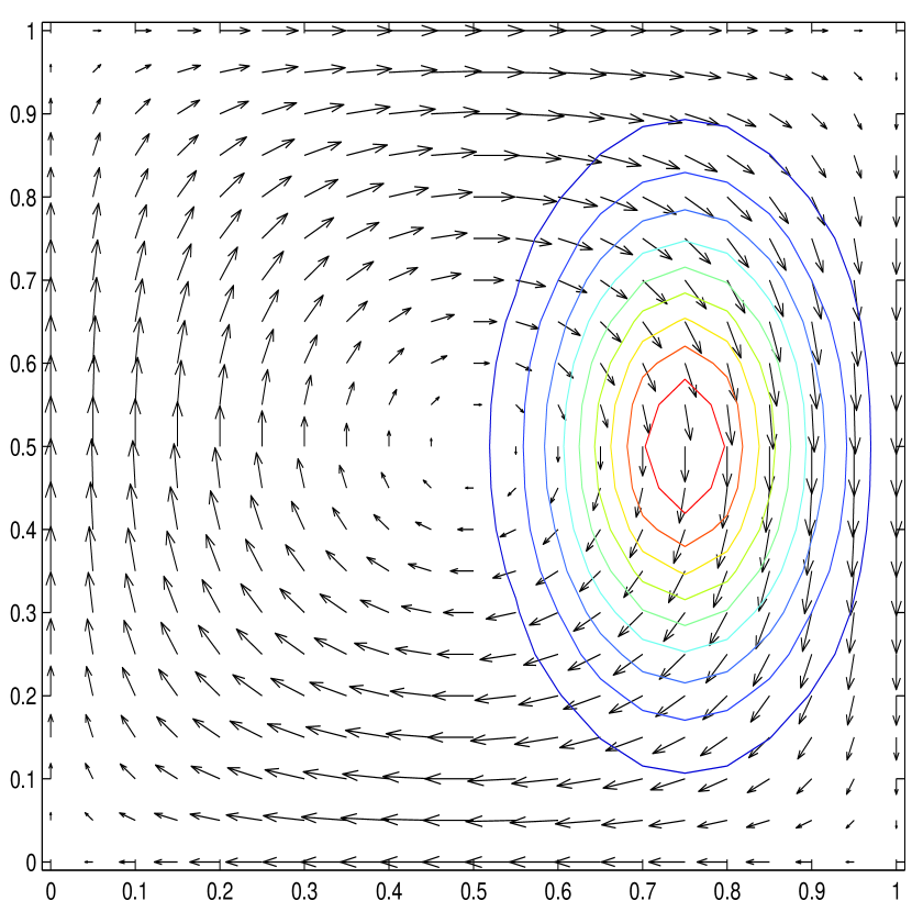
Figure 1: Initial condition for the test problem in Section 4. The contours show level sets of $\omega(0)=\exp(-45(x-{3\over 4})^{2}-15(y-{1\over 2})^{2})$. The arrows show the vector field corresponding to the stream function $\psi=\sin(\pi x)\sin(\pi y)$ by which $\omega$ is advected.

We solve the Liouville equation in $\Omega=[0,1]^{2}$ with initial field $\omega=\exp(-45(x-{3\over 4})^{2}-15(y-{1\over 2})^{2})$ advected by the velocity field with stream function $\psi=\sin(\pi x)\sin(\pi y)$. (See Figure 1.) This velocity field has shear, so $\omega$ rapidly rolls up into a tight spiral, mimicking the filamentation of vorticity in the Euler equations. The spatial derivatives in Eq. (1) are approximated by the Arakawa Jacobian, which is second order and preserves discrete analogues of energy and enstrophy. Although the discrete enstrophy $\sum\omega_{i}^{2}$ is preserved, this does not help the scheme preserve areas any better than (nonconservative) central differences do.

Particles at the maximum of $\omega$ have a period of about 0.75. We integrate with a second order method for 400 times steps of $\Delta t=0.003$, or total time $1.2$, during which this maximum rotates 1.6 times around the centre of the square $\Omega$. Spatial errors completely dominate the total error at $t=1.2$.

Without any projection, oscillations rapidly develop and the distribution of vorticity values is not maintained at all well (see Figure 3(a)). A large minimum of $\psi=-0.69$ forms, next to a spurious local maximum of $\psi=0.46$. The initial maximum of 1 has not been preserved but has decayed to 0.87. The comparison between the initial and final area functions (see Figure 2) shows that the area within most vorticity contours is not preserved at all.

The area-preserving methods both involve periodically remapping the vorticity. If this period is too short (e.g. one time step), then the cell rearrangement model cannot update the vorticity at all. If it is too long, then not only the area but also the topology of the level sets can alter, which can not be corrected by the present methods. Once a small island of vorticity has been created, for example, it must be advected by the flow.

We first consider the cell rearrangement model of section 2. Suppose the remapping is applied every $N_{r}$ time steps. This needs a large $N_{r}$ to yield a reasonably smooth remapped vorticity field; but if $N_{r}$ is too large then spurious maxima can evolve which are not removed by the remapping. With no remapping, this maximum reaches $0.46$. With $N_{r}=50$, it reaches $0.26$. With $N_{r}=20$, there is no isolated spurious maximum, but oscillations start to appear within the main island. These grow worse at $N_{r}=10$. Therefore, $N_{r}=20$ seems a reasonable balance, and the final field is shown in Figure 3(b). In one remapping period, the central peak moves across about 2 cells.

This remapping is very fast, but it does not maintain smoothness of $\omega$, as can be seen here. In fact, it is surprising that it works even as well as it does in this example. However, the lack of smoothness would not be a problem in problems involving poorly-resolved turbulent fields.

We consider now the vorticity relabelling model of section 3. In this model we are free to decrease the remapping interval $N_{r}$ as desired: we still obtain smooth results with $N_{r}=1$, for example. As $N_{r}$ is decreased, the results progressively improve. For $N_{r}=\infty$, 20, 10, and 5, the peak of the spurious maximum is at $\omega=0.46$, $0.09$, $0.02$, and $0.002$, respectively. (Because of its smooth interpolation, it cannot completely eliminate this maximum, as the cell rearrangement model does.) Results for $N_{r}=10$ are shown in Figure 3(d). The final field is very smooth, considering the coarse $20\times 20$ grid, and very plausibly represents an element of the original state composed with an area-preserving diffeomorphism. One contour of the exact solution (found by particle tracking) is shown in the background. The computed solution has clearly suffered far too much diffusion, a result of using diffusive, non-upwinded second differences to approximate the advection term. Nevertheless, it is impressive that such information can be extracted from the same method that produced Figure 3(a), by merely imposing some conservation laws.

Finally, Figure 3(c), shows the vorticity relabelling model applied to an even simpler spatial discretization, namely ordinary central differences. It is in fact more accurate that the Arakawa Jacobian (Fig. 3(d)), being slightly less diffusive. Thus, preserving areas lets one use much simpler finite differences and still maintain smooth, non-oscillatory solutions.

Any of the techniques presented here can be combined with a more sophisticated underlying Eulerian scheme. If we used a high-order, low-diffusion upwinding scheme, for example, then area errors would have been much less than in Fig. 3(a); but they would still increase over time. Applying the vorticity relabelling would still improve the solution.

5 Discussion

The methods discussed here take into account one large family of conservation laws. This possibility raises many questions. What is the effect of using these methods for very long times? What is their effect on other conservation laws such as energy and symplecticity? How well do they work on larger applications such as the shallow water equations? (For level-set applications, a simpler update, adding a constant to the advected field so that the area inside one particular level set is preserved, may be preferable.)

More theoretically, is it possible to regard the ‘equal area’ functions as defining a discrete phase space in which consistent approximations can be directly derived, instead of using brute force modification of existing methods? While desirable, this looks difficult, since we are not projecting to any well-defined manifold. Consider the subset of $\mbox{\Bbb R}^{N^{2}+1}$ defined by

$$A_{\omega}(\omega_{i})=A_{0}(c),\ i=1,\dots,N^{2}.$$

This does have dimension 1 in general, but is formidably curled up on itself. It may be better to think of the constrained phase space as the configurations lying within some small distance of a manifold of dimension $\mbox{\Bbb R}^{N^{2}-{\cal O}(N)}$, as we are enforcing one curve’s worth of constraints.

Acknowledgements I am extremely grateful to Tom Hou and Arieh Iserles for bringing this problem to my attention, to Reinout Quispel for useful discussions and for providing the reference [7], and to Paul Turner who studied the cell rearrangement model in the course of his M.Sc. thesis [9]. This research is supported by the Marsden Fund of the Royal Society of New Zealand. Part of it was undertaken when the author enjoyed the support of the MSRI, Berkeley. MSRI wishes to acknowledge the support of the NSF through grant no. DMS–9701755.

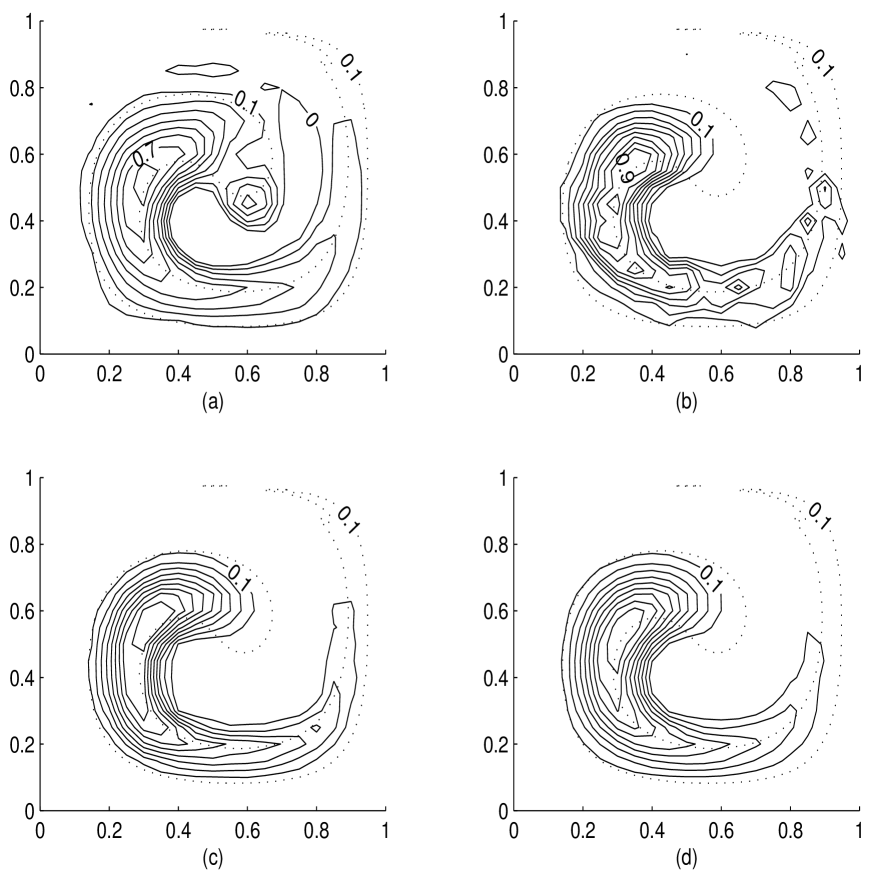
Figure 3: Results for the advection problem on Fig. 1 after 1.6 rotations about the center. (a): Arakawa differences with no area preservation. A large negative blob of vorticity forms and spawns a secondary positive blob. The dotted contour indicates the exact solution. (b): Arakawa differences with cell rearrangement applied every 20 time steps ($\Delta t=0.001$). (c): Central differences with vorticity relabelling applied every 10 time steps. (d) Arakawa differences with vorticity relabelling applied every 10 time steps.

References

- [1] A. Arakawa, Computational design for long-term numerical integration of the equations of fluid motion: two-dimensional incompressible flow. Part I. J. Comput. Phys. 1 (1966) 119–143.
- [2] V. Arnold and B. Khesin, Topological Methods in Hydrodynamics, Springer, New York, 1998.
- [3] P. D. Lax, Approximation of measure preserving transformations, Comm. Pure Appl. Math. 24 (1971), 133–135.
- [4] R. I. McLachlan, Spatial discretization of partial differential equations with integrals, SIAM J. Numer. Anal., submitted.
- [5] R. I. McLachlan and G. R. W. Quispel, Six lectures on the geometric integration of ODEs, preprint at www.massey.ac.nz/ RMcLachl.
- [6] J. E. Marsden and A. Weinstein, Coadjoint orbits, vortices and Clebsch variables for incompressible fluids, Physica D 7 (1983), 305–323.
- [7] P. E. Kloeden and J. Mustard, Construction of permutations approximating Lebesgue measure preserving dynamical systems under spatial discretization, Int. J. Bifurcation and Chaos 7(2) (1997), 401–406.
- [8] J. C. Scovel, On symplectic lattice maps, Phys. Lett. A 159 (1991), 396–400.
- [9] P. G. Turner, Cellular automata model of 2D inviscid fluids, M.Sc. thesis, Massey University, 1997.
- [10] V. Zeitlin, Finite-mode analogues of 2D ideal hydrodynamics: Coadjoint orbits and local canonical structure, Physica D 49 (1991), 353–362.