Abstract

A self-contained description of algebraic structures, obtained by combinations of various limit procedures applied to vertex and face $sl(2)$ elliptic quantum affine algebras, is given. New double Yangians structures of dynamical type are in particular defined. Connections between these structures are established. A number of them take the form of twist-like actions. These are conjectured to be evaluations of universal twists.

MSC number: 81R50, 17B37

LAPTH-738/99

PAR-LPTHE 99-23

DTP-99-45

math.QA/9906189

June 1999

1 Introduction

1.1 Overview

The study of elliptic quantum algebras, defined with the help of elliptic $R$-matrices, has yielded a number of algebraic structures relevant to certain integrable systems in quantum mechanics and statistical mechanics (noticeably the $XYZ$ model [1], RSOS models [2, 3] and Sine–Gordon theory [4, 5]). More recently the definition and construction of some scaling limits has led to the notion of deformed double Yangian algebras. We will investigate and develop here in great detail the occurrence of these and other limit algebraic structures and the pattern of connection in between, in the simplest case of an underlying $sl(2)$ algebra.

Two classes of elliptic solutions to the Yang–Baxter equation have been identified, respectively associated with the vertex statistical models [6, 7] and the face-type statistical models [2, 8, 9]. The vertex elliptic $R$-matrix for $sl(2)$ was first used by Sklyanin [10] to construct a two-parameter deformation of the enveloping algebra ${\cal U}(sl(2))$. The central extension of this structure was proposed in [11] for $sl(2)$, and later extended to ${\cal A}_{q,p}{(\widehat{sl(N)}_{c})}$ in [12]. Its connection to $q$-deformed Virasoro and ${\cal W}_{N}$ algebras [13, 14, 15] was established in [16, 17].

The face-type $R$-matrices, depending on the extra parameters $\lambda$ belonging to the dual of the Cartan algebra in the underlying algebra, were first used by Felder [18] to define the algebra ${{\cal B}_{q,p,\lambda}{(\widehat{sl(2)}_{c})}}$ in the $R$-matrix approach. Enriquez and Felder [19] and Konno [3] introduced a current representation, although differences arise in the treatment of the central extension. A slightly different structure, also based upon face-type $R$-matrices but incorporating extra, Heisenberg algebra generators, was introduced as ${\cal U}_{q,p}(sl(2))$ [3, 20]. This structure is relevant to the resolution of the quantum Calogero–Moser and Ruijsenaar–Schneider models [21, 22, 23]. Another dynamical elliptic algebra, denoted ${\cal A}_{q,p;\pi}{(\widehat{sl(2)}_{c})}$, was also defined and studied in [24]. It was then interpreted, at the level of representation, as a twist of ${{\cal A}_{q,p}{(\widehat{sl(2)}_{c})}}$.

Particular limits of the ${\cal A}_{q,p}$-type algebras were subsequently defined and compared with previously known structures. The limit $p\rightarrow 0$ together with the renormalization of the generators by suitable powers of $p$ before taking the limit, leads to the quantum algebra ${{\cal U}_{q}{(\widehat{sl(2)}_{c})}}$ such as presented in [25, 15]. It differs from the presentation in [26] by a scalar factor in the $R$-matrix. The scaling limit of the algebra ${\cal A}_{q,p;\pi}{(\widehat{sl(2)}_{c})}$ was also defined in [24].

A second limit was considered in [27, 4] ($R$-matrix formulation) and [28] (current algebra formulation). It is defined by taking $p=q^{2r}$ (elliptic nome) and $z=q^{i\beta/\pi}$ (spectral parameter) with $q\rightarrow 1$. This algebra, denoted ${\cal A}_{\hbar,\eta}{(\widehat{sl(2)}_{c})}$, where $\eta\equiv\frac{1}{r}$ and $q\simeq e^{\epsilon\hbar}$ with $\epsilon\rightarrow 0$, is relevant to the study of the $XXZ$ model in its gapless regime [27]. It admits a further limit $r\rightarrow\infty$ ($\eta\rightarrow 0$) where its $R$-matrix becomes identical to the $R$-matrix defining the double Yangian ${{\cal D}Y(sl(2))_{c}}$ (centrally extended), defined in [29] (Yangian double), [30] (central extension); alternative versions with a different normalization are given in [31] (for $sl(2)$) and [32] (for $sl(N)$). This difference in the normalization factors of the $R$-matrix, crucial in confronting the centrally extended versions, is the exact counterpart of the difference between the presentation of ${{\cal U}_{q}{(\widehat{sl(2)}_{c})}}$ in [26] and [25].

One must however be careful in this identification in terms of $R$-matrix structure since the generating functionals (Lax matrices) of these algebras admit different interpretations in terms of modes (generators of the enveloping algebra). In the context of ${\cal A}_{\hbar,0}{(\widehat{sl(2)}_{c})}$ the expansion is done in terms of continuous-index Fourier modes of the spectral parameter (see [4, 28]); in the context of ${{\cal D}Y(sl(2))_{c}}$ the expansion is done in terms of powers of the spectral parameter (see [29, 30, 32]).

It was shown recently that both vertex algebras ${\cal A}_{q,p}{(\widehat{sl(N)}_{c})}$ and face-type algebras ${\cal B}_{q,\lambda}{(\widehat{sl(N)}_{c})}$ were in fact Drinfel’d twists [33] of the quantum group ${\cal U}_{q}{(\widehat{sl(N)}_{c})}$. Originating with the proposition of [22] on face-type algebras, the construction of the twist operators was undertaken in both cases by Frønsdal [34, 35] and finally achieved at the level of formal universal twists in [12, 36]. In [36], the universal twist is obtained by solving a linear equation introduced in [37], this equation playing a fundamental rôle for complex continuation of $6j$ symbols. Moreover in the case of finite (super)algebras, the convergence of the infinite products defining the twists was also proved in [36]. This led to a formal construction of universal $R$-matrices for the elliptic algebras ${\cal A}_{q,p}$ and ${\cal B}_{q,\lambda}$, of which the BB and ABF $4\!\times\!4$ matrices are respectively (spin $1/2$) evaluation representations.

1.2 General settings

Our strategy is to combine in as many patterns as possible the different limit procedures introduced previously in the literature; to apply them to cases not already considered, in particular the face type algebras ${{\cal B}_{q,p,\lambda}{(\widehat{sl(2)}_{c})}}$; and thus to achieve as large as possible a self-contained network of algebraic structures extending from the elliptic quantum affine algebras to the affine Lie algebra ${{\cal U}{(\widehat{sl(2)}_{c})}}$.

Before summarizing our investigations, we must first of all define precisely the concepts which we will use throughout this paper, so that no ambiguity arises in our statements.

We shall deal with formal algebraic structures defined by $R$-matrix exchange relations between formal $2\!\times\!2$ matrix-valued generating functionals denoted Lax operators, using the well-known $RLL$ formalism [38]. Explicit $R$-matrices here are interpreted as evaluation representations of universal objects whenever they are known to exist, or conjectural universal objects when not. We shall not give any precise definition of the individual generators themselves, i.e. the specific expression of the individual generators in terms of spectral parameter dependent Lax operators. These definitions would eventually give rise to the fully explicit algebraic structure. For instance we shall not distinguish here between the double Yangian ${{\cal D}Y(sl(2))_{c}}$ and the scaled algebra ${\cal A}_{\hbar,0}{(\widehat{sl(2)}_{c})}$. Definition of, and identification between algebraic structures will therefore be understood at the sole level of their $R$-matrix presentation, except in explicitly specified cases where we are able to state relations between the full (generator-described) exchange structures, or even the Hopf or quasi-Hopf algebraic structures. We consider that the existence of such relations is in any case an indication that similar connections exist at the level of universal algebras, to be explicitly formulated once the explicit algebra generators are defined.

Similarly we shall manipulate $R$-matrices at the level of their evaluation representation of spin $1/2$ ($4\!\times\!4$ matrices). Only when we shall use the term “universal”, will it mean the abstract algebraic object known as universal $R$-matrix. The same will apply to twist operators connecting (quasi)-Hopf algebraic structures [33], and the $R$-matrices of the algebras. We recall that a twist operator $F$ lives in the square ${\cal A}^{\otimes 2}$ of an algebraic structure; it connects two coproducts in ${\cal A}$ as $\Delta_{F}(\cdot)=F\Delta(\cdot)F^{-1}$, and two universal $R$-matrices as $R_{F}=F^{\pi}RF^{-1}$. Its evaluation representation acts similarly on the evaluation representation of the universal $R$-matrices:

$$R^{F}_{12}=F_{21}R_{12}F^{-1}_{12}\;.$$ (1.1)

As in the previous case of identifications of algebras, we conjecture that occurrence of a relation of this form at the level of evaluated $R$-matrices is an indication that a similar relation exists at the level of universal algebras. We shall therefore denote any such relation between evaluated $R$-matrices as a “twist-like action” between two algebraic structures respectively characterized by $R$ and $R^{F}$, even when we do not have explicit proof that a universal twist exists between the universal $R$-matrices, or the respective coproduct structures.

A connection of the form (1.1) where $F$ will not depend on any parameter (spectral ($z$ or $\beta$, elliptic ($p$ or $r$) or dynamical ($w$ or $s$)) will be termed “rigid twist action”.

We must also introduce the notion of homothetical twist-like connection, whereby we mean the existence of an invertible matrix $F(z)$ such that two $R$-matrices are connected by

$$\widetilde{R}=f(z,p,q)F_{21}(z^{-1})RF_{12}(z)^{-1}\;,$$ (1.2)

where $f(z,p,q)$ is a $c$-number function.
At this point, we do not have an interpretation of this kind of relation between algebraic structure. We shall come back to this point in the conclusion.

1.3 General properties of $R$-matrices and twists

All evaluated $R$-matrices in this paper will obey one of the following equations, implying the associativity of the exchange algebra.

• Yang–Baxter equation:

  $$R_{12}(z)\,R_{13}(zz^{\prime})\,R_{23}(z^{\prime})=R_{23}(z^{\prime})\,R_{13}(zz^{\prime})\,R_{12}(z)\;,$$ (1.3)

  $$R_{12}(\beta)\,R_{13}(\beta+\beta^{\prime})\,R_{23}(\beta^{\prime})=R_{23}(\beta^{\prime})\,R_{13}(\beta+\beta^{\prime})\,R_{12}(\beta)\;,$$ (1.4)

• Dynamical Yang–Baxter equation:

  $$R_{12}(z,\lambda+h^{(3)})\,R_{13}(zz^{\prime},\lambda)\,R_{23}(z^{\prime},\lambda+h^{(1)})=R_{23}(z^{\prime},\lambda)\,R_{13}(zz^{\prime},\lambda+h^{(2)})\,R_{12}(z,\lambda)\;,$$ (1.5)

  $$R_{12}(\beta,\lambda+h^{(3)})\,R_{13}(\beta+\beta^{\prime},\lambda)\,R_{23}(\beta^{\prime},\lambda+h^{(1)})=R_{23}(\beta^{\prime},\lambda)\,R_{13}(\beta+\beta^{\prime},\lambda+h^{(2)})\,R_{12}(\beta,\lambda)\;,$$ (1.6)

depending upon the multiplicative or additive nature of the spectral parameter.

Among the algebraic structures which we consider here, some are known to have Quasitriangular Hopf Algebra (QTHA)  structure (for instance ${{\cal U}_{q}{(\widehat{sl(2)}_{c})}}$, ${{\cal D}Y(sl(2))_{c}}$) [39], and others are Quasitriangular Quasi-Hopf Algebra (QTQHA) [33] (for instance ${{\cal A}_{q,p}{(\widehat{sl(2)}_{c})}}$, ${{\cal B}_{q,p,\lambda}{(\widehat{sl(2)}_{c})}}$).

Their universal $R$-matrices obey the universal Yang–Baxter equation in the first case,

$${\cal R}_{12}{\cal R}_{13}{\cal R}_{23}={\cal R}_{23}{\cal R}_{13}{\cal R}_{12}$$ (1.7)

and a more complicated Yang–Baxter-type equation in the second case, involving a cocycle $\Phi\in{\mathfrak{A}}\otimes{\mathfrak{A}}\otimes{\mathfrak{A}}$:

$${\cal R}_{12}\Phi_{312}{\cal R}_{13}\Phi_{132}^{-1}{\cal R}_{23}\Phi_{123}=\Phi_{321}{\cal R}_{23}\Phi_{231}^{-1}{\cal R}_{13}\Phi_{213}{\cal R}_{12}\;.$$ (1.8)

However, in all the cases which are considered here, the $R$-matrices, once evaluated, obey the Yang–Baxter or dynamical Yang–Baxter equation.

We now recall the following contingent properties of evaluated $R$-matrices.

• Unitarity:

  $$R_{12}(z)\,R_{21}(z^{-1}) = 1\;,$$

  $$R_{12}(\beta)\,R_{21}(-\beta) = 1\;,$$ (1.9)

• Crossing-symmetry:

  $$\Big{(}R_{12}(x)^{t_{2}}\Big{)}^{-1} = \Big{(}R_{12}(q^{2}x)^{-1}\Big{)}^{t_{2}}\;,$$

  $$\left(R_{12}(\beta)^{t_{2}}\right)^{-1} = \left(R_{12}(\beta-2i\pi)^{-1}\right)^{t_{2}}\;,$$ (1.10)

depending upon the multiplicative or additive nature of the spectral parameter.

The unitarity relation is not satisfied in most cases: the already known evaluated $R$-matrices for ${{\cal A}_{q,p}{(\widehat{sl(2)}_{c})}}$, ${{\cal B}_{q,p,\lambda}{(\widehat{sl(2)}_{c})}}$, ${\cal U}_{q,\lambda}{(\widehat{sl(2)}_{c})}$ only obey the crossing relation (• ‣ 1.3) [40, 12]. We shall meet with $R$-matrices obeying unitarity relations at the end of the paper, but we have no proof that they do correspond to evaluations of universal objects. We shall comment on this in the conclusion.

We have indicated that Universal Twist Operators $\cal F$ transform a coproduct $\Delta$ into another one $\Delta^{\cal F}(\cdot)={\cal F}\Delta(\cdot){\cal F}^{-1}$ and the ${\cal R}$ matrix into ${\cal R}^{\cal F}={\cal F}_{21}{\cal R}{\cal F}_{12}^{-1}$. If now $({\mathfrak{A}},\Delta,{\cal R})$ defines a quasi-triangular Hopf algebra and ${\cal F}$ satisfies the cocycle condition

$${{\cal F}}_{12}(\Delta\otimes id){{\cal F}}={{\cal F}}_{23}(id\otimes\Delta){{\cal F}}\;.$$ (1.11)

$({\mathfrak{A}},\Delta^{\cal F},{\cal R}^{\cal F})$ defines again a quasi-triangular Hopf algebra. If however ${\cal F}$ satisfies no particular cocycle-like relation, $({\mathfrak{A}},\Delta^{\cal F},{{\cal R}}^{\cal F})$ defines a QTQHA: ${\cal R}^{\cal F}$ satisfies then the YB-type equation (1.8). An interesting intermediate structure arises when ${\cal F}$ satisfies a so-called shifted cocycle condition, depending upon a parameter $\lambda$ such that [22, 18]:

$${{\cal F}}_{12}(\lambda)(\Delta\otimes id){{\cal F}}={{\cal F}}_{23}(\lambda+h^{(1)})(id\otimes\Delta){{\cal F}}$$ (1.12)

where $h\in{\mathfrak{A}}$. In this case, ${\cal R}^{\cal F}$ satisfies the dynamical Yang–Baxter equation (1.5).

1.4 Summary

Our paper is divided into two parts.

We shall first of all describe the limit procedures whereby the number of parameters in the $R$-matrix description of the algebra (hence including the spectral parameter) is decreased, starting from either ${{\cal A}_{q,p}{(\widehat{sl(2)}_{c})}}$ or ${{\cal B}_{q,p,\lambda}{(\widehat{sl(2)}_{c})}}$; we shall define the limit algebraic structures in both cases. These limit procedures may go in three (for ${{\cal A}_{q,p}{(\widehat{sl(2)}_{c})}}$) or four (for ${{\cal B}_{q,p,\lambda}{(\widehat{sl(2)}_{c})}}$) directions:

• non elliptic limit: one sends $p$ to 0;

• scaling limit: one sends $q$ to 1, with $p=q^{2r}$, $z=q^{i\beta/\pi}$ ($z=q^{2i\beta/\pi}$ and $w=q^{2s}$ in the face case, where $w$ is related to $\lambda$, see below);

• factorization: one “eliminates” the spectral parameter by a Sklyanin-type factorization. At the level of the universal algebra this corresponds to a degeneracy homomorphism (see [28]). This procedure is only known for vertex algebras at this point. Finite face type algebras however are known and shall be considered here, albeit without an established connection with the affine structures.

• non dynamical limit: in the face case the dynamical parameter $\lambda$ can also be eliminated by a procedure which we shall detail in the main body of the text.

These limit procedures, and combinations thereof, lead to the set of objects described by Figure 1.

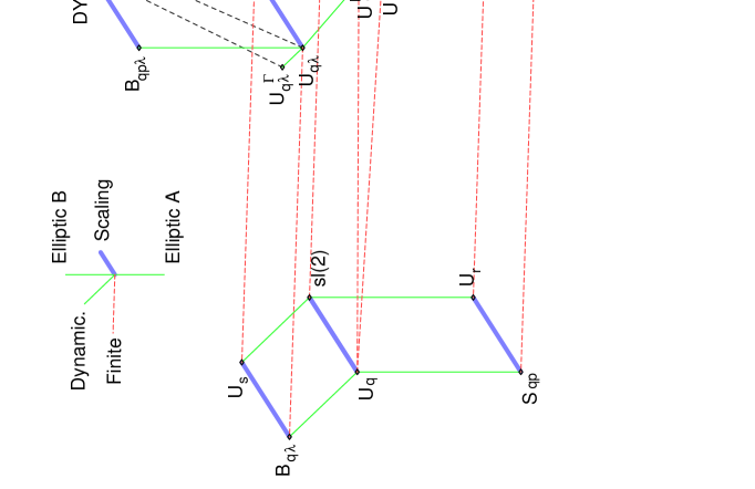
Figure 1: $R$-matrix network

Already known structures are of course present in the diagram: ${{\cal B}_{q,p,\lambda}{(\widehat{sl(2)}_{c})}}$ is the face elliptic, centrally extended algebra; ${{\cal A}_{q,p}{(\widehat{sl(2)}_{c})}}$ is the vertex elliptic, centrally extended algebra; ${\cal U}_{q}^{F}{(\widehat{sl(2)}_{c})}$ and ${\cal U}_{q}^{V}{(\widehat{sl(2)}_{c})}$ are two presentations [40, 12] of the quantum group ${{\cal U}_{q}{(\widehat{sl(2)}_{c})}}$ [25] connected by a conjugation and a twist-like action; ${\cal D}Y_{r}^{V8}{(\widehat{sl(2)}_{c})}$ is the deformed double Yangian algebra ${\cal A}_{\hbar,\eta}{(\widehat{sl(2)}_{c})}$ in [28] with $\hbar=1$ and $\eta=1/r$; ${\cal D}Y_{r}^{V6}{(\widehat{sl(2)}_{c})}$ is the deformed double Yangian algebra defined in [4], connected to the previous one by a rigid twist; ${{\cal D}Y(sl(2))_{c}}$ is the double Yangian defined in [29, 30]; ${\cal U}_{q}(sl(2))$ is the $q$-deformed $sl(2)$ algebra; ${\cal S}_{q,p}(sl(2))$ is Sklyanin’s elliptic “degenerate” algebra, and ${\cal U}_{r}(sl(2))$ is the “degenerate” trigonometric algebra identified with ${\cal U}_{q}(sl(2))$ by $q=e^{i\pi/r}$.

New algebraic structures also appear in this diagram, mostly due to the systematic application of the limit procedures to the face algebra ${{\cal B}_{q,p,\lambda}{(\widehat{sl(2)}_{c})}}$: ${{\cal D}Y_{r,s}(sl(2))_{c}}$ is the scaling limit of ${{\cal B}_{q,p,\lambda}{(\widehat{sl(2)}_{c})}}$; ${{\cal D}Y_{r,s}^{-\infty}(sl(2))_{c}}$ is its $s\ll 0$ limit where the periodic behaviour in $s$ is nevertheless retained; ${{\cal D}Y_{s}(sl(2))_{c}}$ is a dynamical deformation of the double Yangian; ${{\cal U}_{q,\lambda}{(\widehat{sl(2)}_{c})}}$ and ${\cal U}_{q,\lambda}^{\Gamma}{(\widehat{sl(2)}_{c})}$ are dynamical deformations of ${{\cal U}_{q}{(\widehat{sl(2)}_{c})}}$, respectively homothetical to ${{\cal D}Y_{r,s}^{-\infty}(sl(2))_{c}}$ and ${{\cal D}Y_{r,s}(sl(2))_{c}}$ by a suitable redefinition of the parameters; ${{\cal D}Y_{r}^{F}(sl(2))_{c}}$ is an “elliptic” non dynamical deformation of the double Yangian, connected to ${{\cal D}Y_{r}^{V}(sl(2))_{c}}$ by a twist-like action and homothetical to ${{\cal U}_{q}{(\widehat{sl(2)}_{c})}}$ by the same redefinition of the parameters. Finally ${\cal U}_{s}(sl(2))$ and ${\cal B}_{q,\lambda}(sl(2))$ are dynamical deformations of the factorized structures à la Sklyanin, although they themselves are not yet understood as originating from such a factorization. In addition, we also compare the structures resulting from ${{\cal B}_{q,p,\lambda}{(\widehat{sl(2)}_{c})}}$ and the structures derived [24] in the analysis of ${\cal A}_{q,p;\pi}{(\widehat{sl(2)}_{c})}$. These structures are in in fact connected by a TLA which we shall describe.

In order to avoid fastidious repetitions in the body of the text, we state immediately that all these new $R$-matrices have been explicitly checked to obey the Yang–Baxter equation (1.3)–(1.4) or dynamical Yang–Baxter equation (1.5)–(1.6). Such checks are indeed required since the computational procedures which yield these $R$-matrices may entail regularizations of infinite products. This fact in turn potentially invalidates a direct application of these computational procedures to the Yang–Baxter equation originally satisfied by the elliptic $R$-matrices.

In the second part we describe the connections which implement the addition of supplementary parameters. To be precise:

• implementation of the elliptic nome $p$ (or $r$);

• implementation of the dynamical parameter $w$ (or $s$);

• implementation of the quantum parameter $q$ along the scaling limit connections.

Three types of twist-like actions (TLA) appear:

1. TLA explicitely proved to be evaluation of universal twists, represented on the figures 5–7 by a triple arrow. Most of them have been previously established in the literature, particularly in [34, 35, 41, 12].

2. TLA conjectured to be evaluations of universal twists, represented on the figures 5–7 by a double arrow. All these objects are new. They are either deduced from previously known ones by limit procedures or combinations; or explicitly computed from scratch.

3. Homothetical TLA. These are also new; they connect either the affine Lie algebra ${{\cal U}{(\widehat{sl(2)}_{c})}}$ with double Yangian or ${{\cal U}_{q}{(\widehat{sl(2)}_{c})}}$; or they act as reciprocal of the scaling transformations on the vertex or face side. By contrast, let us point out that the first two implementations (of $p$ and $w$ – or $r$ and $s$) are achieved in all cases by twist-like actions.

We finally give some indications on further possible investigations in the conclusion.

Part I Structures and Limits

2 Vertex type algebras

We will start from the elliptic algebra ${{\cal A}_{q,p}{(\widehat{sl(2)}_{c})}}$ and take the above described different limits to obtain various quantum algebras and deformed double Yangians.

2.1 Elliptic algebra ${{\cal A}_{q,p}{(\widehat{sl(2)}_{c})}}$

Let us consider the following $R$-matrix [6, 11]:

$$R(z,q,p)=\frac{\tau(q^{1/2}z^{-1})}{\mu(z)}\left(\begin{array}[]{cccc}a(u)&0&0&d(u)\\ 0&b(u)&c(u)&0\\ 0&c(u)&b(u)&0\\ d(u)&0&0&a(u)\\ \end{array}\right)$$ (2.1)

where

$$a(u)=\frac{\mathop{\rm snh}\nolimits(v-u)}{\mathop{\rm snh}\nolimits(v)}=z^{-1}\;\frac{\Theta_{p^{2}}(q^{2}z^{2})\;\Theta_{p^{2}}(pq^{2})}{\Theta_{p^{2}}(pq^{2}z^{2})\;\Theta_{p^{2}}(q^{2})}\;,$$ (2.2)

$$b(u)=\frac{\mathop{\rm snh}\nolimits(u)}{\mathop{\rm snh}\nolimits(v)}=qz^{-1}\;\frac{\Theta_{p^{2}}(z^{2})\;\Theta_{p^{2}}(pq^{2})}{\Theta_{p^{2}}(pz^{2})\;\Theta_{p^{2}}(q^{2})}\;,$$ (2.3)

$$c(u)=1\;,$$ (2.4)

$$d(u)=-k\,\mathop{\rm snh}\nolimits(v-u)\mathop{\rm snh}\nolimits(u)=-p^{1/2}q^{-1}z^{-2}\;\frac{\Theta_{p^{2}}(z^{2})\;\Theta_{p^{2}}(q^{2}z^{2})}{\Theta_{p^{2}}(pz^{2})\;\Theta_{p^{2}}(pq^{2}z^{2})}\;.$$ (2.5)

The function $\mathop{\rm snh}\nolimits(u)$ is defined by $\mathop{\rm snh}\nolimits(u)=-i\mathop{\rm sn}\nolimits(iu)$ where $\mathop{\rm sn}\nolimits(u)$ is Jacobi’s elliptic function with modulus $k$. The variables $z,q,p$ are related to the variables $u,v$ by

$$p=\exp\Big{(}-\frac{\pi K^{\prime}}{K}\Big{)}\;,\qquad q=-\exp\Big{(}-\frac{\pi v}{2K}\Big{)}\;,\qquad z=\exp\Big{(}\frac{\pi u}{2K}\Big{)}\;,$$ (2.6)

where the elliptic integrals $K,K^{\prime}$ are given by (with ${k^{\prime}}^{2}=1-k^{2}$):

$$K=\int_{0}^{1}\frac{dx}{\sqrt{(1-x^{2})(1-k^{2}x^{2})}}\qquad\mbox{and}\qquad K^{\prime}=\int_{0}^{1}\frac{dx}{\sqrt{(1-x^{2})(1-{k^{\prime}}^{2}x^{2})}}\;.$$ (2.7)

From now on, we shall consider $a$, $b$, $c$, $d$, as functions of $z$ given by (2.6).
The normalization factors are

$$\frac{1}{\mu(z)}=\frac{1}{\kappa(z^{2})}\;\frac{(p^{2};p^{2})_{\infty}}{(p;p)_{\infty}^{2}}\;\frac{\Theta_{p^{2}}(pz^{2})\;\Theta_{p^{2}}(q^{2})}{\Theta_{p^{2}}(q^{2}z^{2})}\;,$$ (2.8)

$$\frac{1}{\kappa(z^{2})}=\frac{(q^{4}z^{-2};p,q^{4})_{\infty}\;(q^{2}z^{2};p,q^{4})_{\infty}\;(pz^{-2};p,q^{4})_{\infty}\;(pq^{2}z^{2};p,q^{4})_{\infty}}{(q^{4}z^{2};p,q^{4})_{\infty}\;(q^{2}z^{-2};p,q^{4})_{\infty}\;(pz^{2};p,q^{4})_{\infty}\;(pq^{2}z^{-2};p,q^{4})_{\infty}}\;,$$ (2.9)

$$\tau(q^{1/2}z^{-1})=q^{-1/2}z\;\frac{\Theta_{q^{4}}(q^{2}z^{2})}{\Theta_{q^{4}}(z^{2})}\;,$$ (2.10)

where the infinite multiple products are defined by:

$$(z;p_{1},\dots,p_{m})_{\infty}=\prod_{n_{i}\geq 0}(1-zp_{1}^{n_{1}}\dots p_{m}^{n_{m}})\;.$$ (2.11)

$R$ satisfies the so-called quasi-periodicity property

$$R_{12}(-zp^{\frac{1}{2}})=(\sigma_{1}\otimes\mbox{1I})^{-1}\,R_{21}(z^{-1})^{-1}\,(\sigma_{1}\otimes\mbox{1I})\;.$$ (2.12)

It also obeys the crossing-symmetry property (• ‣ 1.3), but not unitarity (• ‣ 1.3).
This matrix defines the elliptic algebra ${{\cal A}_{q,p}{(\widehat{sl(2)}_{c})}}$ as

$$R_{12}(z_{1}/z_{2},q,p)\,L_{1}(z_{1})\,L_{2}(z_{2})=L_{2}(z_{2})\,L_{1}(z_{1})\,R_{12}(z_{1}/z_{2},q,p^{*}=pq^{-2c})\;.$$ (2.13)

2.2 Non elliptic limit: quantum affine algebra ${{\cal U}_{q}{(\widehat{sl(2)}_{c})}}$

Starting from the above $R$-matrix of ${{\cal A}_{q,p}{(\widehat{sl(2)}_{c})}}$, and taking the limit $p\rightarrow 0$, one gets the ${{\cal U}_{q}{(\widehat{sl(2)}_{c})}}$ algebra, with its $R$-matrix given by

$$R_{V}(z)=\rho(z^{2})\left(\begin{array}[]{cccc}1&0&0&0\\ 0&\displaystyle\frac{q(1-z^{2})}{1-q^{2}z^{2}}&\displaystyle\frac{z(1-q^{2})}{1-q^{2}z^{2}}&0\\ 0&\displaystyle\frac{z(1-q^{2})}{1-q^{2}z^{2}}&\displaystyle\frac{q(1-z^{2})}{1-q^{2}z^{2}}&0\\ 0&0&0&1\\ \end{array}\right)\;.$$ (2.14)

The normalization factor is

$$\rho(z^{2})=q^{-1/2}\;\frac{(q^{2}z^{2};q^{4})_{\infty}^{2}}{(z^{2};q^{4})_{\infty}\;(q^{4}z^{2};q^{4})_{\infty}}\;.$$ (2.15)

It is known [11] that the algebra ${{\cal U}_{q}{(\widehat{sl(2)}_{c})}}$ is only obtained after a suitable renormalization of the generators of ${{\cal A}_{q,p}{(\widehat{sl(2)}_{c})}}$ and a subsequent non-continuous limit $p\to 0$.

The algebra ${{\cal U}_{q}{(\widehat{sl(2)}_{c})}}$ is then defined by the relations

$$R_{12}(z_{1}/z_{2})\,L^{\pm}_{1}(z_{1})\,L^{\pm}_{2}(z_{2}) = L^{\pm}_{2}(z_{2})\,L^{\pm}_{1}(z_{1})\,R_{12}(z_{1}/z_{2})\;,$$ (2.16)

$$R_{12}(q^{c/2}z_{1}/z_{2})\,L^{+}_{1}(z_{1})\,L^{-}_{2}(z_{2}) = L^{-}_{2}(z_{2})\,L^{+}_{1}(z_{1})\,R_{12}(q^{-c/2}z_{1}/z_{2})\;.$$ (2.17)

As indicated in the introduction, we do not discuss the problem of generator expansions here. The same caveat will hold throughout the whole paper, viz. we shall assume that suitable, consistent expansions of the Lax equations will exist to generate well-defined algebraic structures.

2.3 Scaling limit

The so-called scaling limit of an algebra will be understood as the algebra defined by the scaling limit of the $R$-matrix of the initial structure. It is obtained by setting in the $R$-matrix $p=q^{2r}$ (elliptic nome) and $z=q^{i\beta/\pi}$ (spectral parameter) with $q\rightarrow 1$, and $r$, $\beta$ being kept fixed. The spectral parameter in the Lax operator is now to be taken as $\beta$.

2.3.1 Deformed double Yangian ${{\cal D}Y_{r}^{V8}(sl(2))_{c}}$

Taking the scaling limit of ${{\cal A}_{q,p}{(\widehat{sl(2)}_{c})}}$, one gets the ${{\cal D}Y_{r}^{V8}(sl(2))_{c}}$ algebra. Its $R$-matrix takes the form [4, 42] (the superscript $V8$ is a token of the eight non vanishing entries of the vertex-type $R$-matrix):

$$R_{V8}(\beta,r)=\rho_{V8}(\beta;r)\left(\begin{array}[]{cccc}\displaystyle\frac{\cos\frac{i\beta}{2r}\;\cos\frac{\pi}{2r}}{\cos\frac{\pi+i\beta}{2r}}&0&0&\displaystyle-\frac{\sin\frac{i\beta}{2r}\;\sin\frac{\pi}{2r}}{\cos\frac{\pi+i\beta}{2r}}\\ 0&\displaystyle\frac{\sin\frac{i\beta}{2r}\;\cos\frac{\pi}{2r}}{\sin\frac{\pi+i\beta}{2r}}&\displaystyle\frac{\cos\frac{i\beta}{2r}\;\sin\frac{\pi}{2r}}{\sin\frac{\pi+i\beta}{2r}}&0\\ 0&\displaystyle\frac{\cos\frac{i\beta}{2r}\;\sin\frac{\pi}{2r}}{\sin\frac{\pi+i\beta}{2r}}&\displaystyle\frac{\sin\frac{i\beta}{2r}\;\cos\frac{\pi}{2r}}{\sin\frac{\pi+i\beta}{2r}}&0\\ \displaystyle-\frac{\sin\frac{i\beta}{2r}\;\sin\frac{\pi}{2r}}{\cos\frac{\pi+i\beta}{2r}}&0&0&\displaystyle\frac{\cos\frac{i\beta}{2r}\;\cos\frac{\pi}{2r}}{\cos\frac{\pi+i\beta}{2r}}\\ \end{array}\right)\;.$$ (2.18)

The normalization factor is

$$\rho_{V8}(\beta;r)=-\frac{S_{2}(-\frac{i\beta}{\pi}\;|\;r,2)\,S_{2}(1+\frac{i\beta}{\pi}\;|\;r,2)}{S_{2}(\frac{i\beta}{\pi}\;|\;r,2)\,S_{2}(1-\frac{i\beta}{\pi}\;|\;r,2)}\mathop{\rm cotan}\nolimits\frac{i\beta}{2}\;.$$ (2.19)

$S_{2}(x|\omega_{1},\omega_{2})$ is the Barnes’ double sine function of periods $\omega_{1}$ and $\omega_{2}$ defined by [43], quoted in [44]:

$$S_{2}(x|\omega_{1},\omega_{2})=\frac{\Gamma_{2}(\omega_{1}+\omega_{2}-x\;|\;\omega_{1},\omega_{2})}{\Gamma_{2}(x\;|\;\omega_{1},\omega_{2})}$$ (2.20)

where $\Gamma_{r}$ is the multiple Gamma function of order $r$ given by

$$\Gamma_{r}(x|\omega_{1},\dots,\omega_{r})=\exp\left(\frac{\partial}{\partial s}\sum_{n_{1},\dots,n_{r}\geq 0}(x+n_{1}\omega_{1}+\dots+n_{r}\omega_{r})^{-s}\Bigg{|}_{s=0}\right)\;.$$ (2.21)

This ${R}$ matrix satisfies the quasi-periodicity property

$${R}_{12}(\beta-i\pi r)=(\sigma_{1}\otimes\mbox{1I})^{-1}\,{R}_{21}(-\beta)^{-1}\,(\sigma_{1}\otimes\mbox{1I})\;,$$ (2.22)

where $\sigma_{1}$ is the usual Pauli matrix.
It also obeys the crossing-symmetry property (• ‣ 1.3), but not (• ‣ 1.3).

The algebra ${{\cal D}Y_{r}^{V8}(sl(2))_{c}}$ is then defined by the relation

$$R_{12}(\beta_{1}-\beta_{2},r)\,L_{1}(\beta_{1})\,L_{2}(\beta_{2})=L_{2}(\beta_{2})\,L_{1}(\beta_{1})\,R_{12}(\beta_{1}-\beta_{2},r-c)\;.$$ (2.23)

2.3.2 Double Yangian ${{\cal D}Y(sl(2))_{c}}$

Starting now from the quantum affine algebra ${{\cal U}_{q}{(\widehat{sl(2)}_{c})}}$ and taking its scaling limit, one obtains the double Yangian algebra ${{\cal D}Y(sl(2))_{c}}$ [29]. Its $R$-matrix is given by

$$R(\beta)=\rho(\beta)\left(\begin{array}[]{cccc}1&0&0&0\\ 0&\displaystyle\frac{i\beta}{i\beta+\pi}&\displaystyle\frac{\pi}{i\beta+\pi}&0\\[8.5359pt] 0&\displaystyle\frac{\pi}{i\beta+\pi}&\displaystyle\frac{i\beta}{i\beta+\pi}&0\\ 0&0&0&1\\ \end{array}\right)\;.$$ (2.24)

The normalization factor is

$$\rho(\beta)=\frac{\Gamma_{1}(\frac{i\beta}{\pi}\;|\;2)\;\Gamma_{1}(2+\frac{i\beta}{\pi}\;|\;2)}{\Gamma_{1}(1+\frac{i\beta}{\pi}\;|\;2)^{2}}\;.$$ (2.25)

Taking the limit $r\rightarrow\infty$ of the $R$-matrix of ${{\cal D}Y_{r}^{V8}(sl(2))_{c}}$ (corresponding to the previous $p\rightarrow 0$ limit), one also gets the double Yangian algebra.

Notice that in both previous cases, the limit procedure may be applied directly to the Lax matrices, leading to the explicit, continuous labelled algebras, respectively denoted ${{\cal A}_{\hbar,\eta}{(\widehat{sl(2)}_{c})}}$ and ${{\cal A}_{\hbar,0}{(\widehat{sl(2)}_{c})}}$ [28].

The different limit procedures in the vertex case are summarized in Figure 2.

Figure 2: The vertex case diagram: limit procedures

2.4 Finite algebras

Up to now, the various limits led to affine structures. We now consider another kind of limit where the algebra is “factorized”. The resulting structure is based on a finite $sl(2)$ algebra. This is interpreted as a highly degenerate consistent representation of the affine algebras at $c=0$, where all generators are expressed in terms of only four ones.

2.4.1 Sklyanin algebra

The Sklyanin algebra [10] is constructed from ${{\cal A}_{q,p}{(\widehat{sl(2)}_{c})}}$ taken at $c=0$. The $R$-matrix (2.1) can be written as

$$R(z)=\mbox{1I}\otimes\mbox{1I}+\sum_{\alpha=1}^{3}W_{\alpha}(z)\sigma_{\alpha}\otimes\sigma_{\alpha}\;,$$ (2.26)

where $\sigma_{\alpha}$ are the Pauli matrices and $W_{\alpha}(z)$ are expressed in terms of the Jacobi elliptic functions. A particular $z$-dependence of the $L(z)$ operators is chosen, leading to a factorization of the $z$-dependence in the $RLL$ relations. Indeed, setting

$$L(z)=S_{0}+\sum_{\alpha=1}^{3}W_{\alpha}(z)S_{\alpha}\sigma_{\alpha}\;,$$ (2.27)

one obtains an algebra with four generators $S^{\alpha}$ ($\alpha=0,...,3$) and commutation relations

$$[S_{0},S_{\alpha}] = -iJ_{\beta\gamma}(S_{\beta}S_{\gamma}+S_{\gamma}S_{\beta})\;,$$

$${}[S_{\alpha},S_{\beta}] = i(S_{0}S_{\gamma}+S_{\gamma}S_{0})\;,$$ (2.28)

where $J_{\alpha\beta}=\displaystyle\frac{W_{\alpha}^{2}-W_{\beta}^{2}}{W_{\gamma}^{2}-1}$ and $\alpha$, $\beta$, $\gamma$ are cyclic permutations of 1, 2, 3. The structure functions $J_{\alpha\beta}$ are actually independent of $z$. Hence we get an algebra where the $z$-dependence has been dropped out.

2.4.2 ${\cal U}_{r}(sl(2))$

The same factorization procedure (2.26-2.27) applied to ${{\cal D}Y_{r}^{V8}(sl(2))_{c}}$ leads to a ${\cal U}_{r}(sl(2))$ algebra described by (2.28) with now $J_{12}=-J_{31}=\tan^{2}\frac{\pi}{2r}$ and $J_{23}=0$. We recognize the algebra ${\cal U}_{q^{\prime}}(sl(2))$ if we set $q^{\prime}=e^{i\pi/r}$.

Remark: The scaling limit of the Sklyanin algebra (2.28) also leads to the algebra ${\cal U}_{r}(sl(2))$.

2.4.3 Other factorizations

Applying the factorization procedure (2.26-2.27) to the quantum affine algebra ${{\cal U}_{q}{(\widehat{sl(2)}_{c})}}$, one simply gets the finite ${\cal U}_{q}(sl(2))$ algebra.
Let us remark that this algebra is also the $p\rightarrow 0$ limit of the Sklyanin algebra.

If we finally apply the factorization procedure to the double Yangian ${{\cal D}Y(sl(2))_{c}}$, one gets $J_{\alpha\beta}=0$. Setting the central generator $S_{0}$ to 1, we recognize the classical ${\cal U}(sl(2))$ algebra.

Note that ${\cal U}(sl(2))$ can also be viewed as:

i) the $r\rightarrow\infty$ limit of ${\cal U}_{r}(sl(2))$;

ii) the $q\rightarrow 1$ limit (“scaling limit”) of ${\cal U}_{q}(sl(2))$.

The different limit procedures in the finite vertex case are summarized in figure 3.

Figure 3: The finite vertex case diagram: limit procedures

3 Face type algebras

3.1 Elliptic algebra ${{\cal B}_{q,p,\lambda}{(\widehat{sl(2)}_{c})}}$

The starting point in the face case is the ${{\cal B}_{q,p,\lambda}{(\widehat{sl(2)}_{c})}}$ algebra. Let $\{h,c,d\}$ be a basis of the Cartan subalgebra of ${(\widehat{sl(2)}_{c})}$. If $r,s,s^{\prime}$ are complex numbers, we set $\lambda={{\textstyle{\frac{1}{2}}}}\;(s+1)h+s^{\prime}c+(r+2)d$. The elliptic parameter $p$ and the dynamical parameter $w$ are related to the deformation parameter $q$ by $p=q^{2r}$, $w=q^{2s}$.
The $R$ matrix of ${{\cal B}_{q,p,\lambda}{(\widehat{sl(2)}_{c})}}$ is [18, 12]

$$R(z;p,w)=\rho(z;p)\left(\begin{array}[]{cccc}1&0&0&0\\ 0&b(z)&c(z)&0\\ 0&{\bar{c}}(z)&{\bar{b}}(z)&0\\ 0&0&0&1\\ \end{array}\right)$$ (3.1)

where

$$b(z) = q\frac{(pw^{-1}q^{2};p)_{\infty}\;(pw^{-1}q^{-2};p)_{\infty}}{(pw^{-1};p)_{\infty}^{2}}\;\frac{\Theta_{p}(z)}{\Theta_{p}(q^{2}z)}\;,$$ (3.2)

$${\bar{b}}(z) = q\frac{(wq^{2};p)_{\infty}\;(wq^{-2};p)_{\infty}}{(w;p)_{\infty}^{2}}\;\frac{\Theta_{p}(z)}{\Theta_{p}(q^{2}z)}\;,$$ (3.3)

$$c(z) = \frac{\Theta_{p}(q^{2})}{\Theta_{p}(w)}\;\frac{\Theta_{p}(wz)}{\Theta_{p}(q^{2}z)}\;,$$ (3.4)

$${\bar{c}}(z) = z\frac{\Theta_{p}(q^{2})}{\Theta_{p}(pw^{-1})}\;\frac{\Theta_{p}(pw^{-1}z)}{\Theta_{p}(q^{2}z)}\;.$$ (3.5)

The normalization factor is

$$\rho(z;p)=q^{-1/2}\frac{(q^{2}z;p,q^{4})_{\infty}^{2}}{(z;p,q^{4})_{\infty}\;(q^{4}z;p,q^{4})_{\infty}}\;\frac{(pz^{-1};p,q^{4})_{\infty}\;(pq^{4}z^{-1};p,q^{4})_{\infty}}{(pq^{2}z^{-1};p,q^{4})_{\infty}^{2}}\;.$$ (3.6)

The elliptic algebra ${{\cal B}_{q,p,\lambda}{(\widehat{sl(2)}_{c})}}$ is then defined by [18, 12]

$$R_{12}(z_{1}/z_{2},\lambda+h)\,L_{1}(z_{1},\lambda)\,L_{2}(z_{2},\lambda+h^{(1)})=L_{2}(z_{2},\lambda)\,L_{1}(z_{1},\lambda+h^{(2)})\,R_{12}(z_{1}/z_{2},\lambda)\;.$$ (3.7)

3.2 Dynamical quantum affine algebras ${{\cal U}_{q,\lambda}{(\widehat{sl(2)}_{c})}}$

Starting from the ${{\cal B}_{q,p,\lambda}{(\widehat{sl(2)}_{c})}}$ $R$-matrix, and taking the limit $p\rightarrow 0$, one gets the ${{\cal U}_{q,\lambda}{(\widehat{sl(2)}_{c})}}$ one.
The $R$ matrix of ${{\cal U}_{q,\lambda}{(\widehat{sl(2)}_{c})}}$ is

$$R(z;w)=\rho(z)\left(\begin{array}[]{cccc}1&0&0&0\\ 0&\displaystyle\frac{q(1-z)}{1-q^{2}z}&\displaystyle\frac{(1-q^{2})(1-wz)}{(1-q^{2}z)(1-w)}&0\\ 0&\displaystyle\frac{(1-q^{2})(z-w)}{(1-q^{2}z)(1-w)}&\displaystyle\frac{q(1-z)}{(1-q^{2}z)}\,\frac{(1-wq^{2})(1-wq^{-2})}{(1-w)^{2}}&0\\ 0&0&0&1\\ \end{array}\right)\;.$$ (3.8)

The normalization factor is

$$\rho(z)=q^{-1/2}\;\frac{(q^{2}z;q^{4})_{\infty}^{2}}{(z;q^{4})_{\infty}\;(q^{4}z;q^{4})_{\infty}}\;.$$ (3.9)

3.3 Non dynamical limit

Taking the limit $w\rightarrow 0$ in ${{\cal U}_{q,\lambda}{(\widehat{sl(2)}_{c})}}$, one gets the algebra ${{\cal U}_{q}{(\widehat{sl(2)}_{c})}}$ with $R$-matrix:

$$R_{F}(z)=\rho(z)\left(\begin{array}[]{cccc}1&0&0&0\\ 0&\displaystyle\frac{q(1-z)}{1-q^{2}z}&\displaystyle\frac{1-q^{2}}{1-q^{2}z}&0\\ 0&\displaystyle\frac{z(1-q^{2})}{1-q^{2}z}&\displaystyle\frac{q(1-z)}{1-q^{2}z}&0\\ 0&0&0&1\\ \end{array}\right)\;.$$ (3.10)

The normalization factor is

$$\rho(z)=q^{-1/2}\;\frac{(q^{2}z;q^{4})_{\infty}^{2}}{(z;q^{4})_{\infty}\;(q^{4}z;q^{4})_{\infty}}\;.$$ (3.11)

Remark 1: The matrix (2.14) differs from the matrix (3.10) by rescaling $z\rightarrow z^{2}$ and symmetrization between the $e_{12}\otimes e_{21}$ and $e_{21}\otimes e_{12}$ terms. The corresponding algebraic structures will be denoted respectively ${{\cal U}^{F}_{q}{(\widehat{sl(2)}_{c})}}$ for (3.10) and ${{\cal U}^{V}_{q}{(\widehat{sl(2)}_{c})}}$ for (2.14).

Actually, the matrix $R(z)$ is computed from the universal ${\cal R}$ matrix of ${{\cal U}_{q}{(\widehat{sl(2)}_{c})}}$ by $R(z)=(\pi\otimes\pi){\cal R}(z)$ where $\pi$ is a spin $1/2$ evaluation representation [40]. Implementation of the spectral parameter $z$ in the universal ${\cal R}$ matrix is obtained by

$${\cal R}(z) = Ad(z^{\rho}\otimes 1){\cal R}\qquad\mbox{in the vertex case,}$$ (3.12)

$${\cal R}(z) = Ad(z^{d}\otimes 1){\cal R}\qquad\mbox{in the face case.}$$ (3.13)

Hence, the $R$ matrix of ${{\cal U}^{V}_{q}{(\widehat{sl(2)}_{c})}}$ is associated to the principal gradation of the ${(\widehat{sl(2)}_{c})}$ algebra, whilst the $R$ matrix ${{\cal U}^{F}_{q}{(\widehat{sl(2)}_{c})}}$ is associated to the homogeneous gradation.

Remark 2: The scaling limit of the $R$-matrix (3.10) of ${{\cal U}^{F}_{q}{(\widehat{sl(2)}_{c})}}$ gives back the $R$-matrix (2.24) of ${{\cal D}Y(sl(2))_{c}}$.

3.4 Dynamical deformed double Yangian ${{\cal D}Y_{r,s}(sl(2))_{c}}$

Starting again from the ${{\cal B}_{q,p,\lambda}{(\widehat{sl(2)}_{c})}}$ case, and taking now the scaling limit $p=q^{2r}$ (elliptic nome), $z=q^{2i\beta/\pi}$ (spectral parameter), $w=q^{2s}$ (dynamical parameter) with $q\rightarrow 1$, one gets a new structure, interpreted as a dynamical deformed centrally extended double Yangian ${{\cal D}Y_{r,s}(sl(2))_{c}}$.
The $R$ matrix of ${{\cal D}Y_{r,s}(sl(2))_{c}}$ is

$$R(\beta;r,s)=\rho(\beta;r)\left(\begin{array}[]{cccc}1&0&0&0\\ 0&b(\beta)&c(\beta)&0\\ 0&{\bar{c}}(\beta)&{\bar{b}}(\beta)&0\\ 0&0&0&1\\ \end{array}\right)\;,$$ (3.14)

where

$$b(\beta) = \frac{\Gamma_{1}(r-s\;|\;r)^{2}}{\Gamma_{1}(r-s+1\;|\;r)\,\Gamma_{1}(r-s-1\;|\;r)}\;\frac{\sin\frac{i\beta}{r}}{\sin\frac{\pi+i\beta}{r}}\;,$$ (3.15)

$$c(\beta) = \frac{\sin\frac{\pi s+i\beta}{r}}{\sin\frac{\pi s}{r}}\;\frac{\sin\frac{\pi}{r}}{\sin\frac{\pi+i\beta}{r}}\;,$$ (3.16)

$${\bar{b}}(\beta) = \frac{\Gamma_{1}(s\;|\;r)^{2}}{\Gamma_{1}(s+1\;|\;r)\,\Gamma_{1}(s-1\;|\;r)}\;\frac{\sin\frac{i\beta}{r}}{\sin\frac{\pi+i\beta}{r}}\;,$$ (3.17)

$${\bar{c}}(\beta) = \frac{\sin\frac{\pi s-i\beta}{r}}{\sin\frac{\pi s}{r}}\;\frac{\sin\frac{\pi}{r}}{\sin\frac{\pi+i\beta}{r}}\;.$$ (3.18)

The normalization factor is the same as formula (2.19), rewritten as

$$\rho(\beta;r)=\frac{S_{2}^{2}(1+\frac{i\beta}{\pi}\;|\;r,2)}{S_{2}(\frac{i\beta}{\pi}\;|\;r,2)\,S_{2}(2+\frac{i\beta}{\pi}\;|\;r,2)}\;.$$ (3.19)

The algebra ${{\cal D}Y_{r,s}(sl(2))_{c}}$ is then defined by the relations

$$R_{12}(\beta_{1}-\beta_{2},\lambda+h)\,L_{1}(\beta_{1},\lambda)\,L_{2}(\beta_{2},\lambda+h^{(1)})=L_{2}(\beta_{2},\lambda)\,L_{1}(\beta_{1},\lambda+h^{(2)})\,R_{12}(\beta_{1}-\beta_{2},\lambda)\;.$$ (3.20)

3.5 Dynamical double Yangian ${{\cal D}Y_{s}(sl(2))_{c}}$

Taking the limit $r\rightarrow\infty$ in ${{\cal D}Y_{r,s}(sl(2))_{c}}$, one gets a new, dynamical, centrally extended double Yangian ${{\cal D}Y_{s}(sl(2))_{c}}$.
The $R$ matrix of ${{\cal D}Y_{s}(sl(2))_{c}}$ is given by

$$R(\beta)=\rho(\beta)\left(\begin{array}[]{cccc}1&0&0&0\\ 0&\displaystyle\frac{i\beta}{i\beta+\pi}&\displaystyle\frac{\pi s+i\beta}{s(i\beta+\pi)}&0\\ 0&\displaystyle\frac{\pi s-i\beta}{s(i\beta+\pi)}&\displaystyle\frac{s^{2}-1}{s^{2}}\,\frac{i\beta}{i\beta+\pi}&0\\ 0&0&0&1\\ \end{array}\right)\;.$$ (3.21)

The normalization factor is

$$\rho(\beta)=\frac{\Gamma_{1}(\frac{i\beta}{\pi}\;|\;2)\;\Gamma_{1}(2+\frac{i\beta}{\pi}\;|\;2)}{\Gamma_{1}(1+\frac{i\beta}{\pi}\;|\;2)^{2}}\;.$$ (3.22)

Remark 1: This $R$-matrix (3.21) is also obtained by taking the scaling limit of the $R$-matrix (3.8) of ${{\cal U}_{q,\lambda}{(\widehat{sl(2)}_{c})}}$.

Remark 2: The $|s|\rightarrow\infty$ limit of the $R$-matrix (3.21) gives back the $R$-matrix (2.24) of ${{\cal D}Y(sl(2))_{c}}$.

3.6 Dynamical deformed double Yangian ${{\cal D}Y_{r,s}^{-\infty}(sl(2))_{c}}$ in the trigonometric limit

Starting again from ${{\cal D}Y_{r,s}(sl(2))_{c}}$ and taking $s\ll 0$, but retaining the oscillating behaviour in $s$, one gets ${{\cal D}Y_{r,s}^{-\infty}(sl(2))_{c}}$, another dynamical deformed centrally extended double Yangian structure.
The $R$ matrix of ${{\cal D}Y_{r,s}^{-\infty}(sl(2))_{c}}$ reads

$$R(\beta;r,s)=\rho(\beta;r)\left(\begin{array}[]{cccc}1&0&0&0\\ 0&\displaystyle\frac{\sin\frac{i\beta}{r}}{\sin\frac{\pi+i\beta}{r}}&\displaystyle\frac{\sin\frac{\pi s+i\beta}{r}}{\sin\frac{\pi s}{r}}\;\frac{\sin\frac{\pi}{r}}{\sin\frac{\pi+i\beta}{r}}&0\\ 0&\quad\displaystyle\frac{\sin\frac{\pi s-i\beta}{r}}{\sin\frac{\pi s}{r}}\;\frac{\sin\frac{\pi}{r}}{\sin\frac{\pi+i\beta}{r}}&\quad\displaystyle\frac{\sin\pi\frac{s+1}{r}\sin\pi\frac{s-1}{r}}{\sin^{2}\frac{\pi s}{r}}\frac{\sin\frac{i\beta}{r}}{\sin\frac{\pi+i\beta}{r}}&0\\ 0&0&0&1\\ \end{array}\right)\;.$$ (3.23)

The normalization factor is the same as for ${{\cal D}Y_{r,s}(sl(2))_{c}}$, see (3.19).

Remark 1: The limit $r\rightarrow\infty$ of the $R$-matrix (3.23) gives again the $R$-matrix (3.21) of ${{\cal D}Y_{s}(sl(2))_{c}}$.

Remark 2: Correspondence with ${{\cal U}_{q,\lambda}{(\widehat{sl(2)}_{c})}}$
The previous $R$ matrix is homothetical to that of ${{\cal U}_{q,\lambda}{(\widehat{sl(2)}_{c})}}$ by the following identifications of parameters:

$$z=e^{-2\beta/r}\;,\qquad q=e^{i\pi/r}\;,\qquad w=e^{2i\pi s/r}\;.$$ (3.24)

The same identification of parameters applied to the $R$-matrix (3.14) of ${{\cal D}Y_{r,s}(sl(2))_{c}}$ leads to an $R$-matrix close to that of ${{\cal U}_{q,\lambda}{(\widehat{sl(2)}_{c})}}$, but with $\Gamma$-function dependence in the dynamical parameter. This would define a new dynamical algebraic structure ${\cal U}^{\Gamma}_{q,\lambda}{(\widehat{sl(2)}_{c})}$.

3.7 Deformed double Yangian ${{\cal D}Y_{r}^{F}(sl(2))_{c}}$

Taking now the limit $s\rightarrow i\infty$ in ${{\cal D}Y_{r,s}(sl(2))_{c}}$, one gets a non dynamical structure ${{\cal D}Y_{r}^{F}(sl(2))_{c}}$.
The $R$ matrix of ${{\cal D}Y_{r}^{F}(sl(2))_{c}}$ is given by

$$R(\beta;r)=\rho(\beta;r)\left(\begin{array}[]{cccc}1&0&0&0\\ 0&\displaystyle\frac{\sin\frac{i\beta}{r}}{\sin\frac{\pi+i\beta}{r}}&e^{\beta/r}\displaystyle\frac{\sin\frac{\pi}{r}}{\sin\frac{\pi+i\beta}{r}}&0\\ 0&\quad e^{-\beta/r}\displaystyle\frac{\sin\frac{\pi}{r}}{\sin\frac{\pi+i\beta}{r}}&\quad\displaystyle\frac{\sin\frac{i\beta}{r}}{\sin\frac{\pi+i\beta}{r}}&0\\ 0&0&0&1\\ \end{array}\right)\;.$$ (3.25)

The normalization factor is the same as for ${{\cal D}Y_{r,s}(sl(2))_{c}}$.

Remark 1: The limit $r\rightarrow\infty$ of the $R$-matrix (3.25) gives again the $R$-matrix of ${{\cal D}Y(sl(2))_{c}}$.

Remark 2: Correspondence with ${{\cal U}_{q}{(\widehat{sl(2)}_{c})}}$
This matrix is homothetical to that of ${{\cal U}_{q}{(\widehat{sl(2)}_{c})}}$ – eq. (3.10) – by the following identifications of parameters:

$$z=e^{-2\beta/r}\;,\qquad q=e^{i\pi/r}\;.$$ (3.26)

The different limit procedures in the face case are summarized in Figure 4.

Figure 4: The face case diagram: limit procedures

3.8 Finite dimensional algebras

By constrast with the vertex case, the finite face-type elliptic algebras have not yet been obtained from the affine algebras by a factorization procedure. The starting point of our description will therefore be the $R$-matrix representation of ${\cal B}_{q,\lambda}(sl(2))$ given in [41].

3.8.1 Elliptic algebra ${\cal B}_{q,\lambda}(sl(2))$

The $R$-matrix of ${\cal B}_{q,\lambda}(sl(2))$ is

$$R(w)=q^{-1/2}\left(\begin{array}[]{cccc}1&0&0&0\\ 0&q&\displaystyle\frac{1-q^{2}}{1-w}&0\\ 0&\displaystyle-\frac{w(1-q^{2})}{1-w}&\displaystyle\;\frac{q(1-wq^{2})(1-wq^{-2})}{(1-w)^{2}}&0\\ 0&0&0&1\\ \end{array}\right)\;.$$ (3.27)

Remark: The limit $w\rightarrow 0$ of this matrix gives the usual $R$-matrix of ${\cal U}_{q}(sl(2))$

$$R=q^{-1/2}\left(\begin{array}[]{cccc}1&0&0&0\\ 0&q&1-q^{2}&0\\ 0&0&q&0\\ 0&0&0&1\\ \end{array}\right)\;.$$ (3.28)

3.8.2 Dynamical algebra ${\cal U}_{s}(sl(2))$

Taking the scaling limit $w=q^{2s}$ with $q\rightarrow 1$, we obtain the dynamical algebra ${\cal U}_{s}(sl(2))$ with the $R$-matrix

$$R=\left(\begin{array}[]{cccc}1&0&0&0\\ 0&1&s^{-1}&0\\ 0&-s^{-1}&1-s^{-2}&0\\ 0&0&0&1\\ \end{array}\right)\;.$$ (3.29)

The limit $|s|\rightarrow\infty$ of (3.29) gives 1I, which is the evaluated $R$-matrix of ${\cal U}(sl(2))$. It is not clear to us whether this particular matrix (3.29) can be used for an $RLL$ formulation of the algebra. However, we will show in the second part that it is indeed obtained as evaluation of a universal twist action on the universal $R$-matrix $1\otimes 1$ of ${\cal U}(sl(2))$.

Part II Twist operations

We now describe the twist connections between the various algebraic structures previously defined. We first discuss twist-like actions between vertex-type algebras; we then introduce TLAs between ${{\cal U}^{V}_{q}{(\widehat{sl(2)}_{c})}}$ and ${{\cal U}^{F}_{q}{(\widehat{sl(2)}_{c})}}$. We then give the TLA between face-like algebras. The TLAs are classified here according to the “arrival” algebraic structure, i.e. with the highest number of parameters. We end up with the homothetical TLAs.

4 Vertex type algebras

4.1 Twist operator ${{\cal U}^{V}_{q}{(\widehat{sl(2)}_{c})}}\rightarrow{{\cal A}_{q,p}{(\widehat{sl(2)}_{c})}}$

The existence of a twist operator between ${{\cal U}^{V}_{q}{(\widehat{sl(2)}_{c})}}$ and ${{\cal A}_{q,p}{(\widehat{sl(2)}_{c})}}$ was proved at the level of universal matrices in [12]. Once the operators are evaluated, one gets

$${R}[{{\cal A}_{q,p}{(\widehat{sl(2)}_{c})}}]=E^{(1)}_{21}(z^{-1};p)\;R[{{\cal U}^{V}_{q}{(\widehat{sl(2)}_{c})}}]\;{E^{(1)}_{12}}(z;p)^{-1}\;.$$ (4.1)

The twist operator $E^{(1)}(z;p)$ is given by [34, 35]

$$E^{(1)}(z;p)=\rho_{E}(z;p)\left(\begin{array}[]{cccc}a_{E}(z)&0&0&d_{E}(z)\\ 0&b_{E}(z)&c_{E}(z)&0\\ 0&c_{E}(z)&b_{E}(z)&0\\ d_{E}(z)&0&0&a_{E}(z)\\ \end{array}\right)\;,$$ (4.2)

where

$$a_{E}(z)\pm d_{E}(z) = \frac{(\mp p^{1/2}qz;p)_{\infty}}{(\mp p^{1/2}q^{-1}z;p)_{\infty}}$$ (4.3)

$$b_{E}(z)\pm c_{E}(z) = \frac{(\mp pqz;p)_{\infty}}{(\mp pq^{-1}z;p)_{\infty}}\;.$$ (4.4)

The normalization factor is

$$\rho_{E}(z;p)=\frac{(pz^{2};p,q^{4})_{\infty}\;(pq^{4}z^{2};p,q^{4})_{\infty}}{(pq^{2}z^{2};p,q^{4})_{\infty}^{2}}\;.$$ (4.5)

4.2 Deformed double Yangians ${{\cal D}Y_{r}^{V}(sl(2))_{c}}$

4.2.1 Deformed double Yangian ${{\cal D}Y_{r}^{V6}(sl(2))_{c}}$

We need to define an algebraic structure not previously derived in this paper.
The $R$ matrix (2.18) of the deformed double Yangian ${{\cal D}Y_{r}^{V8}(sl(2))_{c}}$ can be related to the two-body $S$ matrix of the Sine–Gordon theory $S_{SG}(\beta,r)$ by a rigid twist operator. The connection goes as follows. One defines the following $R$-matrix [4]:

$$R_{V6}(\beta,r)=\mathop{\rm cotan}\nolimits(\frac{i\beta}{2})S_{SG}(\beta,r)=\rho_{V6}(\beta;r)\left(\begin{array}[]{cccc}1&0&0&0\\[2.84526pt] 0&\displaystyle\frac{\sin\frac{i\beta}{r}}{\sin\frac{\pi+i\beta}{r}}&\displaystyle\frac{\sin\frac{\pi}{r}}{\sin\frac{\pi+i\beta}{r}}&0\\[14.22636pt] 0&\displaystyle\frac{\sin\frac{\pi}{r}}{\sin\frac{\pi+i\beta}{r}}&\displaystyle\frac{\sin\frac{i\beta}{r}}{\sin\frac{\pi+i\beta}{r}}&0\\[14.22636pt] 0&0&0&1\\ \end{array}\right)\;,$$ (4.6)

where $\rho_{V6}(\beta;r)=\rho_{V8}(\beta;r)$, see (2.19). This $R$-matrix is assumed to define by the $RLL$ formalism an algebraic structure denoted ${{\cal D}Y_{r}^{V6}(sl(2))_{c}}$.
One has now

$$R[{{\cal D}Y_{r}^{V8}(sl(2))_{c}}]=K_{21}\;R[{{\cal D}Y_{r}^{V6}(sl(2))_{c}}]\;K_{12}^{-1}\;.$$ (4.7)

The rigid twist operator $K$ is given by

$$K=\frac{1}{2}\left(\begin{array}[]{rrrr}1&-i&-i&-1\\ -1&-i&i&-1\\ -1&i&-i&-1\\ 1&i&i&-1\\ \end{array}\right)\;.$$ (4.8)

Remark 1: We note that

$$K=V\otimes V\qquad\mbox{with}\qquad V=\frac{1}{\sqrt{2}}\left(\begin{array}[]{rr}1&-i\\ -1&-i\\ \end{array}\right)\;.$$ (4.9)

This implies an isomorphism between ${{\cal D}Y_{r}^{V8}(sl(2))_{c}}$ and ${{\cal D}Y_{r}^{V6}(sl(2))_{c}}$ where the Lax operators are connected by $L_{V8}=VL_{V6}V^{-1}$.

Remark 2: The rigid twist leaves invariant the $R$-matrix of the undeformed double Yangian, upon which $V$ induces an automorphism.

Remark 3: The $R$ matrix (4.6) is homothetical to that of ${{\cal U}^{V}_{q}{(\widehat{sl(2)}_{c})}}$ – eq. (2.14) – by the following identifications of parameters:

$$z=e^{-\beta/r}\;,\qquad q=e^{i\pi/r}\;.$$ (4.10)

Remark 4: By applying the twist $K$ to the $R$-matrix (2.14) we obtain an $R$-matrix $R[{\cal U}^{V8}_{q}{(\widehat{sl(2)}_{c})}]$ with eight non-vanishing entries which may equivalently describe ${{\cal U}_{q}{(\widehat{sl(2)}_{c})}}$ according to remark 1.
Moreover, $R[{\cal U}^{V8}_{q}{(\widehat{sl(2)}_{c})}]$ appears to be homothetical to the $R$-matrix obtained by redefining the parameters of (2.18) according to (4.10).

4.2.2 Twist operator ${{\cal D}Y(sl(2))_{c}}\rightarrow{{\cal D}Y_{r}^{V8}(sl(2))_{c}}$

The $R$-matrix of ${{\cal D}Y_{r}^{V8}(sl(2))_{c}}$ can be obtained from the $R$-matrix of ${{\cal D}Y(sl(2))_{c}}$ by a twist-like action:

$${R}[{{\cal D}Y_{r}^{V8}(sl(2))_{c}}]=E^{(2)}_{21}(-\beta;r)\;R[{{\cal D}Y(sl(2))_{c}}]\;{E^{(2)}_{12}}(\beta;r)^{-1}\;.$$ (4.11)

The twist operator $E^{(2)}(\beta;r)$ is the scaling limit of the twist operator $E^{(1)}(z,p)$, see eq. (4.2). It is given by

$$E^{(2)}(\beta;r)=\rho_{E}(\beta;r)\left(\begin{array}[]{cccc}a_{E}(\beta)&0&0&d_{E}(\beta)\\ 0&b_{E}(\beta)&c_{E}(\beta)&0\\ 0&c_{E}(\beta)&b_{E}(\beta)&0\\ d_{E}(\beta)&0&0&a_{E}(\beta)\\ \end{array}\right)\;,$$ (4.12)

where

$$a_{E}(\beta)+d_{E}(\beta) = 1\;,$$ (4.13)

$$a_{E}(\beta)-d_{E}(\beta) = \frac{\Gamma_{1}(r-1+\frac{i\beta}{\pi}\;|\;2r)}{\Gamma_{1}(r+1+\frac{i\beta}{\pi}\;|\;2r)}\;,$$ (4.14)

$$b_{E}(\beta)+c_{E}(\beta) = 1\;,$$ (4.15)

$$b_{E}(\beta)-c_{E}(\beta) = \frac{\Gamma_{1}(2r-1+\frac{i\beta}{\pi}\;|\;2r)}{\Gamma_{1}(2r+1+\frac{i\beta}{\pi}\;|\;2r)}\;.$$ (4.16)

The normalization factor is

$$\rho_{E}(\beta;r)=\frac{\Gamma_{2}(r+1+\frac{i\beta}{\pi}\;|\;r,2)^{2}}{\Gamma_{2}(r+\frac{i\beta}{\pi}\;|\;r,2)\;\Gamma_{2}(r+2+\frac{i\beta}{\pi}\;|\;r,2)}\;.$$ (4.17)

4.2.3 Twist operator ${{\cal D}Y(sl(2))_{c}}\rightarrow{{\cal D}Y_{r}^{V6}(sl(2))_{c}}$

Combining the previous two twist-like actions, one gets

$${R}[{{\cal D}Y_{r}^{V6}(sl(2))_{c}}]=E^{(3)}_{21}(-\beta;r)\;R[{{\cal D}Y(sl(2))_{c}}]\;E^{(3)}_{12}(\beta;r)^{-1}\;.$$ (4.18)

The twist operator $E^{(3)}(\beta;r)$ is given by $E^{(3)}=K^{-1}E^{(2)}$, that is

$$E^{(3)}(\beta;r)={{\textstyle{\frac{1}{2}}}}\;\rho_{E}(\beta;r)\left(\begin{array}[]{cccc}1&-1&-1&1\\ i(a_{E}-d_{E})(\beta)&i(b_{E}-c_{E})(\beta)&i(c_{E}-b_{E})(\beta)&i(d_{E}-a_{E})(\beta)\\ i(a_{E}-d_{E})(\beta)&i(c_{E}-b_{E})(\beta)&i(b_{E}-c_{E})(\beta)&i(d_{E}-a_{E})(\beta)\\ -1&-1&-1&-1\\ \end{array}\right)\;,$$ (4.19)

where $a_{E},b_{E},c_{E},d_{E}$ are given by the formulae (4.13)–(4.16) and the normalization factor $\rho_{E}(\beta;r)$ by (4.17).

The different twist procedures in the vertex case are summarized in Figure 5.

5 Vertex to face isomorphism

The two $R$ matrices (2.14) and (3.10) can be related by a twist operator:

$$R[{{\cal U}^{F}_{q}{(\widehat{sl(2)}_{c})}}](z^{2})=K^{(6)}_{21}(z^{-1})\;R[{{\cal U}^{V}_{q}{(\widehat{sl(2)}_{c})}}](z)\;{K^{(6)}_{12}(z)}^{-1}\;.$$ (5.1)

The twist operator $K^{(6)}$ is given by

$$K^{(6)}(z)=\left(\begin{array}[]{cccc}1&0&0&0\\ 0&z^{-1/2}&0&0\\ 0&0&z^{1/2}&0\\ 0&0&0&1\\ \end{array}\right)=\left(\begin{array}[]{cc}1&0\\ 0&z^{1/2}\end{array}\right)\otimes\left(\begin{array}[]{cc}1&0\\ 0&z^{-1/2}\end{array}\right)\;.$$ (5.2)

which acts also as a bona fide conjugation since $K_{21}(z^{-1})=K_{12}(z)$. Moreover, a redefinition of the Lax operators in (2.16,2.17) as

$$L_{F}^{-}(z^{2}) = \left(\begin{array}[]{cc}z^{-1/2}&0\\ 0&z^{1/2}\end{array}\right)L_{V}^{-}(z)\left(\begin{array}[]{cc}z^{1/2}&0\\ 0&z^{-1/2}\end{array}\right)$$ (5.7)

$$L_{F}^{+}(z^{2}) = \left(\begin{array}[]{cc}z^{-1/2}q^{-c/4}&0\\ 0&z^{1/2}q^{c/4}\end{array}\right)L_{V}^{+}(z)\left(\begin{array}[]{cc}z^{1/2}q^{-c/4}&0\\ 0&z^{-1/2}q^{c/4}\end{array}\right)$$ (5.12)

provides a genuine algebra isomorphism between ${{\cal U}^{F}_{q}{(\widehat{sl(2)}_{c})}}$ and ${{\cal U}^{V}_{q}{(\widehat{sl(2)}_{c})}}$.

6 Face type algebras

6.1 Twist operator ${{\cal U}^{F}_{q}{(\widehat{sl(2)}_{c})}}\rightarrow{{\cal U}_{q,\lambda}{(\widehat{sl(2)}_{c})}}$

The two $R$ matrices of ${{\cal U}^{F}_{q}{(\widehat{sl(2)}_{c})}}$ and ${{\cal U}_{q,\lambda}{(\widehat{sl(2)}_{c})}}$ can be related by a twist operator:

$$R[{{\cal U}_{q,\lambda}{(\widehat{sl(2)}_{c})}}]=F^{(3)}_{21}(w)\;R[{{\cal U}^{F}_{q}{(\widehat{sl(2)}_{c})}}]\;{F^{(3)}_{12}}(w)^{-1}\;.$$ (6.1)

The twist operator $F^{(3)}(w)$ is given by

$$F^{(3)}(w)=\left(\begin{array}[]{cccc}1&0&0&0\\ 0&1&\displaystyle\frac{w(q-q^{-1})}{1-w}&0\\ 0&0&1&0\\ 0&0&0&1\\ \end{array}\right)\;.$$ (6.2)

6.2 Dynamical face elliptic affine algebra ${{\cal B}_{q,p,\lambda}{(\widehat{sl(2)}_{c})}}$

6.2.1 Twist operator ${{\cal U}^{F}_{q}{(\widehat{sl(2)}_{c})}}\rightarrow{{\cal B}_{q,p,\lambda}{(\widehat{sl(2)}_{c})}}$

The existence of a twist operator between ${{\cal U}^{F}_{q}{(\widehat{sl(2)}_{c})}}$ and ${{\cal B}_{q,p,\lambda}{(\widehat{sl(2)}_{c})}}$ was proved at the level of universal matrices in [12]. Once the operators are evaluated, one gets

$$R[{{\cal B}_{q,p,\lambda}{(\widehat{sl(2)}_{c})}}]=F^{(1)}_{21}(z^{-1};p,w)\;R[{{\cal U}^{F}_{q}{(\widehat{sl(2)}_{c})}}]\;{F^{(1)}_{12}}(z;p,w)^{-1}\;.$$ (6.3)

The twist operator $F^{(1)}(z;p,w)$ is given by

$$F^{(1)}(z;p,w)=\rho_{F}(z;p)\left(\begin{array}[]{cccc}1&0&0&0\\ 0&X_{11}(z)&X_{12}(z)&0\\ 0&X_{21}(z)&X_{22}(z)&0\\ 0&0&0&1\\ \end{array}\right)\;,$$ (6.4)

where

$$X_{11}(z) = {{}_{2}\phi_{1}\left(\begin{array}[]{c}{wq^{2}}\quad{q^{2}}\\ {w}\end{array};{p,pq^{-2}z}\right)}\;,$$ (6.7)

$$X_{12}(z) = \frac{w(q-q^{-1})}{1-w}\;{{}_{2}\phi_{1}\left(\begin{array}[]{c}{wq^{2}}\quad{pq^{2}}\\ {pw}\end{array};{p,pq^{-2}z}\right)}\;,$$ (6.10)

$$X_{21}(z) = z\;\frac{pw^{-1}(q-q^{-1})}{1-pw^{-1}}\;{{}_{2}\phi_{1}\left(\begin{array}[]{c}{pw^{-1}q^{2}}\quad{pq^{2}}\\ {p^{2}w^{-1}}\end{array};{p,pq^{-2}z}\right)}\;,$$ (6.13)

$$X_{22}(z) = {{}_{2}\phi_{1}\left(\begin{array}[]{c}{pw^{-1}q^{2}}\quad{q^{2}}\\ {pw^{-1}}\end{array};{p,pq^{-2}z}\right)}\;.$$ (6.16)

The $q$-hypergeometric function ${{}_{2}\phi_{1}\left(\begin{array}[]{c}{q^{a}}\quad{q^{b}}\\ {q^{c}}\end{array};{q,z}\right)}$ is defined by

$${{}_{2}\phi_{1}\left(\begin{array}[]{c}{q^{a}}\quad{q^{b}}\\ {q^{c}}\end{array};{q,z}\right)}=\sum_{n=0}^{\infty}\frac{(q^{a};q)_{n}(q^{b};q)_{n}}{(q^{c};q)_{n}(q;q)_{n}}\;z^{n}\qquad\mathrm{where}\qquad(x;q)_{n}=\prod_{k=0}^{n-1}(1-xq^{k})\;.$$ (6.17)

The normalization factor is

$$\rho_{F}(z;p)=\frac{(pz;p,q^{4})_{\infty}\;(pq^{4}z;p,q^{4})_{\infty}}{(pq^{2}z;p,q^{4})_{\infty}^{2}}\;.$$ (6.18)

6.2.2 Twist operator ${{\cal U}_{q,\lambda}{(\widehat{sl(2)}_{c})}}\rightarrow{{\cal B}_{q,p,\lambda}{(\widehat{sl(2)}_{c})}}$

Combining the last two twist-like actions, one obtains

$$R[{{\cal B}_{q,p,\lambda}{(\widehat{sl(2)}_{c})}}]=F^{(5)}_{21}(z^{-1};p,w)\;R[{{\cal U}_{q,\lambda}{(\widehat{sl(2)}_{c})}}]\;{F^{(5)}_{12}(z;p,w)}^{-1}\;.$$ (6.19)

The twist operator $F^{(5)}(z;p,w)$ is given by $F^{(5)}=F^{(1)}{F^{(3)}}^{-1}$, that is

$$F^{(5)}(z;w)=\rho_{F}(z;p)\left(\begin{array}[]{cccc}1&0&0&0\\ 0&X_{11}^{\prime}(z)&X_{12}^{\prime}(z)&0\\ 0&X_{21}^{\prime}(z)&X_{22}^{\prime}(z)&0\\ 0&0&0&1\\ \end{array}\right)\;,$$ (6.20)

where

$$X^{\prime}_{11}(z) = X_{11}(z)\;,$$ (6.21)

$$X^{\prime}_{12}(z) = X_{12}(z)-\frac{w(q-q^{-1})}{1-w}\;X_{11}(z)\;,$$ (6.22)

$$X^{\prime}_{21}(z) = X_{21}(z)\;,$$ (6.23)

$$X^{\prime}_{22}(z) = X_{22}(z)-\frac{w(q-q^{-1})}{1-w}\;X_{21}(z)\;.$$ (6.24)

and $X_{ij}(z)$ are given in (6.7).
The normalization factor $\rho_{F}(z;p)$ is given by (6.18).

6.3 Dynamical double Yangian ${{\cal D}Y_{s}(sl(2))_{c}}$

By taking the scaling limit of the connection (6.1), one gets

$$R[{{\cal D}Y_{s}(sl(2))_{c}}]=F^{(4)}_{21}(s)\;R[{{\cal D}Y(sl(2))_{c}}]\;{F^{(4)}_{12}}(s)^{-1}\;.$$ (6.25)

The twist operator $F^{(4)}(s)$ is the scaling limit of the twist operator $F^{(3)}$, see eq. (6.2). It is given by

$$F^{(4)}(s)=\left(\begin{array}[]{cccc}1&0&0&0\\ 0&1&-s^{-1}&0\\ 0&0&1&0\\ 0&0&0&1\\ \end{array}\right)\;.$$ (6.26)

6.4 Deformed double Yangian ${{\cal D}Y_{r}^{F}(sl(2))_{c}}$

6.4.1 Twist operator ${{\cal D}Y_{r}^{F}(sl(2))_{c}}$ $\rightarrow{{\cal D}Y_{r}^{V}(sl(2))_{c}}$

The two deformed double Yangians ${{\cal D}Y_{r}^{V}(sl(2))_{c}}$ and ${{\cal D}Y_{r}^{F}(sl(2))_{c}}$ obtained from the vertex type algebras on one hand, and from face type algebras on the other hand, are related by twist-like actions. One has:

$$R[{{\cal D}Y_{r}^{F}(sl(2))_{c}}](\beta)=K^{(6)}_{21}(-\beta)\;R[{{\cal D}Y_{r}^{V6}(sl(2))_{c}}](\beta)\;{K^{(6)}_{12}(\beta)}^{-1}\;.$$ (6.27)

The twist operator $K^{(6)}$ is actually equal to the twist operator (5.2) by setting $z=e^{-\beta/r}$:

$$K^{(6)}(\beta)=\left(\begin{array}[]{cccc}1&0&0&0\\ 0&e^{\beta/2r}&0&0\\ 0&0&e^{-\beta/2r}&0\\ 0&0&0&1\\ \end{array}\right)\;.$$ (6.28)

Using the rigid twist operator (4.8), one gets also:

$$R[{{\cal D}Y_{r}^{F}(sl(2))_{c}}](\beta)=K^{(8)}_{21}(-\beta)\;R[{{\cal D}Y_{r}^{V8}(sl(2))_{c}}](\beta)\;{K^{(8)}_{12}(\beta)}^{-1}\;.$$ (6.29)

The twist operator $K^{(8)}$ is given by $K^{(8)}=K^{(6)}K^{-1}$, that is

$$K^{(8)}(\beta)=\frac{1}{2}\left(\begin{array}[]{cccc}1&-1&-1&1\\ ie^{\beta/2r}&ie^{\beta/2r}&-ie^{\beta/2r}&-ie^{\beta/2r}\\ ie^{-\beta/2r}&-ie^{-\beta/2r}&ie^{-\beta/2r}&-ie^{-\beta/2r}\\ -1&-1&-1&-1\\ \end{array}\right)\;.$$ (6.30)

This twist provides a link between the face type and vertex type double Yangian structures.

6.4.2 Twist operator ${{\cal D}Y(sl(2))_{c}}\rightarrow{{\cal D}Y_{r}^{F}(sl(2))_{c}}$

The connection between $R$-matrices of ${{\cal D}Y(sl(2))_{c}}$ and ${{\cal D}Y_{r}^{F}(sl(2))_{c}}$ can be established by three different combinations of previously constructed twist-like actions. These three combinations of course give by construction the same twist operator $F^{(7)}=K^{(8)}E^{(2)}=K^{(6)}K^{-1}E^{(2)}$. One has therefore

$$R[{{\cal D}Y_{r}^{F}(sl(2))_{c}}]=F^{(7)}_{21}(-\beta;r,)\;R[{{\cal D}Y(sl(2))_{c}}]\;{F^{(7)}_{12}(\beta;r)}^{-1}\;.$$ (6.31)

The twist operator $F^{(7)}$ is given by

$$F^{(7)}(\beta;r)={{\textstyle{\frac{1}{2}}}}\;\rho_{E}(\beta;r)\left(\begin{array}[]{cccc}1&-1&-1&1\\ i(a_{E}-d_{E})e^{\beta/2r}&i(b_{E}-c_{E})e^{\beta/2r}&i(c_{E}-b_{E})e^{\beta/2r}&i(d_{E}-a_{E})e^{\beta/2r}\\ i(a_{E}-d_{E})e^{-\beta/2r}&i(c_{E}-b_{E})e^{-\beta/2r}&i(b_{E}-c_{E})e^{-\beta/2r}&i(d_{E}-a_{E})e^{-\beta/2r}\\ -1&-1&-1&-1\\ \end{array}\right)\;,$$ (6.32)

where $a_{E},b_{E},c_{E},d_{E}$ are given by (4.13)–(4.16) and the normalization factor $\rho_{E}(\beta;r)$ by (4.17).

6.5 Trigonometric Dynamical deformed double Yangian ${{\cal D}Y_{r,s}^{-\infty}(sl(2))_{c}}$

6.5.1 Twist operator ${{\cal D}Y_{r}^{F}(sl(2))_{c}}\rightarrow{{\cal D}Y_{r,s}^{-\infty}(sl(2))_{c}}$

The connection between ${{\cal D}Y_{r}^{F}(sl(2))_{c}}$ and ${{\cal D}Y_{r,s}^{-\infty}(sl(2))_{c}}$ is achieved by the twist operator $F^{(3)}$:

$$R[{{\cal D}Y_{r,s}^{-\infty}(sl(2))_{c}}]=F^{(3)}_{21}(s)\;R[{{\cal D}Y_{r}^{F}(sl(2))_{c}}]\;{F^{(3)}_{12}(s)}^{-1}\;.$$ (6.33)

The twist operator $F^{(3)}$ is actually equal to the twist operator (6.2) by setting $q=e^{i\pi/r}$ and $w=e^{2i\pi s/r}$:

$$F^{(3)}(s)=\left(\begin{array}[]{cccc}1&0&0&0\\ 0&1&-e^{i\pi s/r}\displaystyle\frac{\sin\frac{\pi}{r}}{\sin\frac{\pi s}{r}}&0\\ 0&0&1&0\\ 0&0&0&1\\ \end{array}\right)\;.$$ (6.34)

6.5.2 Twist operator ${{\cal D}Y(sl(2))_{c}}\rightarrow{{\cal D}Y_{r,s}^{-\infty}(sl(2))_{c}}$

Combination of two twist-like operations yields the connection between ${{\cal D}Y(sl(2))_{c}}$ and ${{\cal D}Y_{r,s}^{-\infty}(sl(2))_{c}}$:

$$R[{{\cal D}Y_{r,s}^{-\infty}(sl(2))_{c}}]=F^{(10)}_{21}(-\beta;r,s)\;R[{{\cal D}Y(sl(2))_{c}}]\;{F^{(10)}_{12}(\beta;r,s)}^{-1}\;.$$ (6.35)

The twist operator $F^{(10)}$ is given by $F^{(10)}=F^{(3)}F^{(7)}$, that is

$$F^{(10)}(\beta;r,s)={{\textstyle{\frac{1}{2}}}}\;\rho_{E}(\beta;r)$$

$$\qquad\left(\begin{array}[]{cccc}1&-1&-1&1\\ i(a_{E}-d_{E})e_{+}&i(b_{E}-c_{E})e_{-}&i(c_{E}-b_{E})e_{-}&i(d_{E}-a_{E})e_{+}\\ i(a_{E}-d_{E})e^{-\beta/2r}&i(c_{E}-b_{E})e^{-\beta/2r}&i(b_{E}-c_{E})e^{-\beta/2r}&i(d_{E}-a_{E})e^{-\beta/2r}\\ -1&-1&-1&-1\\ \end{array}\right)$$ (6.40)

where $e_{\pm}=e^{\beta/2r}\mp e^{i\pi s/r}e^{-\beta/2r}\frac{\sin(\pi/r)}{\sin(\pi s/r)}$, the functions $a_{E},b_{E},c_{E},d_{E}$ are given by the formulae (4.13)–(4.16) and the normalization factor $\rho_{E}(\beta;r)$ by (4.17).

6.5.3 Twist operator ${{\cal D}Y_{s}(sl(2))_{c}}\rightarrow{{\cal D}Y_{r,s}^{-\infty}(sl(2))_{c}}$

Again, combination of two twist-like operations yields the connection between ${{\cal D}Y_{s}(sl(2))_{c}}$ and ${{\cal D}Y_{r,s}^{-\infty}(sl(2))_{c}}$:

$$R[{{\cal D}Y_{r,s}^{-\infty}(sl(2))_{c}}]=F^{(8)}_{21}(-\beta;r,s)\;R[{{\cal D}Y_{s}(sl(2))_{c}}]\;{F^{(8)}_{12}(\beta;r,s)}^{-1}\;.$$ (6.42)

The twist operator $F^{(8)}$ is given by $F^{(8)}=F^{(10)}{F^{(4)}}^{-1}$, that is

$$F^{(8)}(\beta;r,s)={{\textstyle{\frac{1}{2}}}}\;\rho_{E}(\beta;r)$$

$$\qquad\left(\begin{array}[]{cccc}1&-1&-1-s^{-1}&1\\ i(a_{E}-d_{E})e_{+}&i(b_{E}-c_{E})e_{-}&i(c_{E}-b_{E})e_{-}(1-s^{-1})&i(d_{E}-a_{E})e_{+}\\ i(a_{E}-d_{E})e^{-\beta/2r}&i(c_{E}-b_{E})e^{-\beta/2r}&i(b_{E}-c_{E})e^{-\beta/2r}(1-s^{-1})&i(d_{E}-a_{E})e^{-\beta/2r}\\ -1&-1&-1-s^{-1}&-1\\ \end{array}\right)$$ (6.47)

(6.48)

where $e_{\pm}$, $a_{E},b_{E},c_{E},d_{E}$ and $\rho_{E}(\beta;r)$ have the same meaning as above.

6.6 Dynamical deformed double Yangian ${{\cal D}Y_{r,s}(sl(2))_{c}}$

6.6.1 Twist operator ${{\cal D}Y_{r,s}^{-\infty}(sl(2))_{c}}\rightarrow{{\cal D}Y_{r,s}(sl(2))_{c}}$

The $R$-matrices of ${{\cal D}Y_{r,s}^{-\infty}(sl(2))_{c}}$ and ${{\cal D}Y_{r,s}(sl(2))_{c}}$ are connected by a diagonal TLA (not depending on the spectral parameter):

$$R[{{\cal D}Y_{r,s}(sl(2))_{c}}]=G_{21}(r,s)\;R[{{\cal D}Y_{r,s}^{-\infty}(sl(2))_{c}}]\;{G_{12}(r,s)}^{-1}\;.$$ (6.49)

The twist operator $G$ is given by

$$G(r,s)=\left(\begin{array}[]{cccc}1&0&0&0\\ 0&g^{-1}&0&0\\ 0&0&g&0\\ 0&0&0&1\\ \end{array}\right)=\left(\begin{array}[]{cc}1&0\\ 0&g\end{array}\right)\otimes\left(\begin{array}[]{cc}1&0\\ 0&g^{-1}\end{array}\right)\;,$$ (6.50)

where

$$g(r,s)=\displaystyle\frac{\Gamma_{1}(r-s\;|\;r)}{\Gamma_{1}(r-s+1\;|\;r)^{1/2}\;\Gamma_{1}(r-s-1\;|\;r)^{1/2}}\;.$$ (6.51)

Remark: Equivalently, $G$ expressed in terms of the parameters $q=e^{i\pi/r}$ and $w=e^{2i\pi s/r}$ realizes a TLA between ${{\cal U}_{q,\lambda}{(\widehat{sl(2)}_{c})}}$ and ${\cal U}^{\Gamma}_{q,\lambda}{(\widehat{sl(2)}_{c})}$ defined in remark 2, Section 3.6.

6.6.2 Twist operator ${{\cal D}Y_{s}(sl(2))_{c}}\rightarrow{{\cal D}Y_{r,s}(sl(2))_{c}}$

Combining the last two twists, one gets:

$$R[{{\cal D}Y_{r,s}(sl(2))_{c}}]=F^{(6)}_{21}(-\beta;r,s)\;R[{{\cal D}Y_{s}(sl(2))_{c}}]\;{F^{(6)}_{12}(\beta;r,s)}^{-1}\;.$$ (6.52)

The twist operator $F^{(6)}$ is given by $F^{(6)}=GF^{(8)}$, that is

$$F^{(6)}(\beta;r,s)={{\textstyle{\frac{1}{2}}}}\;\rho_{E}(\beta;r)$$

$$\left(\begin{array}[]{cccc}1&-1&-1-s^{-1}&1\\ i(a_{E}-d_{E})e_{+}g^{-1}&i(b_{E}-c_{E})e_{-}g^{-1}&i(c_{E}-b_{E})e_{-}(1-s^{-1})g^{-1}&i(d_{E}-a_{E})e_{+}g^{-1}\\ i(a_{E}-d_{E})e^{-\beta/2r}g&i(c_{E}-b_{E})e^{-\beta/2r}g&i(b_{E}-c_{E})e^{-\beta/2r}(1-s^{-1})g&i(d_{E}-a_{E})e^{-\beta/2r}g\\ -1&-1&-1-s^{-1}&-1\\ \end{array}\right)$$ (6.57)

where $e_{\pm}$, $a_{E},b_{E},c_{E},d_{E}$ and $\rho_{E}(\beta;r)$ have the same meaning as above and $g$ is given by (6.51).

6.6.3 Twist operator ${{\cal D}Y(sl(2))_{c}}\rightarrow{{\cal D}Y_{r,s}(sl(2))_{c}}$

Similarly, by a combination of previous twists, one gets:

$$R[{{\cal D}Y_{r,s}(sl(2))_{c}}]=F^{(2)}_{21}(-\beta;r,s)\;R[{{\cal D}Y(sl(2))_{c}}]\;{F^{(2)}_{12}(\beta;r,s)}^{-1}\;.$$ (6.59)

The twist operator $F^{(2)}$ is given by $F^{(2)}=GF^{(10)}$, that is

$$F^{(2)}(\beta;r,s)={{\textstyle{\frac{1}{2}}}}\;\rho_{E}(\beta;r)$$

$$\qquad\left(\begin{array}[]{cccc}1&-1&-1&1\\ i(a_{E}-d_{E})e_{+}g^{-1}&i(b_{E}-c_{E})e_{-}g^{-1}&i(c_{E}-b_{E})e_{-}g^{-1}&i(d_{E}-a_{E})e_{+}g^{-1}\\ i(a_{E}-d_{E})e^{-\beta/2r}g&i(c_{E}-b_{E})e^{-\beta/2r}g&i(b_{E}-c_{E})e^{-\beta/2r}g&i(d_{E}-a_{E})e^{-\beta/2r}g\\ -1&-1&-1&-1\\ \end{array}\right)$$ (6.64)

where $e_{\pm}$, $a_{E},b_{E},c_{E},d_{E}$ and $\rho_{E}(\beta;r)$ have the same meaning as above and $g$ is given by (6.51).

6.6.4 Twist operator ${{\cal D}Y_{r}^{F}(sl(2))_{c}}\rightarrow{{\cal D}Y_{r,s}(sl(2))_{c}}$

Finally, connection between ${{\cal D}Y_{r}^{F}(sl(2))_{c}}$ and ${{\cal D}Y_{r,s}(sl(2))_{c}}$ is provided by

$$R[{{\cal D}Y_{r,s}(sl(2))_{c}}]=F^{(11)}_{21}(r,s)\;R[{{\cal D}Y_{r}^{F}(sl(2))_{c}}]\;{F^{(11)}_{12}(r,s)}^{-1}\;.$$ (6.66)

The twist operator $F^{(11)}$ is given by $F^{(11)}=GF^{(3)}$, that is

$$F^{(11)}(r,s)=\left(\begin{array}[]{cccc}1&0&0&0\\ 0&g^{-1}&-e^{i\pi s/r}\displaystyle\frac{\sin\frac{\pi}{r}}{\sin\frac{\pi s}{r}}\,g^{-1}&0\\ 0&0&g&0\\ 0&0&0&1\\ \end{array}\right)\;,$$ (6.67)

where $g$ is given by (6.51).

The different twist procedures in the face case are summarized in Figure 6.

6.7 Connections with ${\cal A}_{q,p;\pi}{(\widehat{sl(2)}_{c})}$ and derived algebras

6.7.1 Twist ${{\cal B}_{q,p,\lambda}{(\widehat{sl(2)}_{c})}}\to{{\cal A}}_{q,p;\pi}{(\widehat{sl(2)}_{c})}$

The $R$-matrix of ${\cal A}_{q,p;\pi}{(\widehat{sl(2)}_{c})}$ given in [24] (actually their $R^{+}$-matrix) is

$$R=z^{1/2r}\rho(z)\left(\begin{array}[]{cccc}1&0&0&0\\[2.84526pt] 0&\displaystyle\frac{\Theta_{p}(z)\Theta_{p}(q^{-2}w)}{\Theta_{p}(q^{2}z)\Theta_{p}(w)}&\displaystyle\frac{\Theta_{p}(zw)\Theta_{p}(q^{2})}{\Theta_{p}(q^{2}z)\Theta_{p}(w)}&0\\[14.22636pt] 0&\displaystyle\frac{\Theta_{p}(z^{-1}w)\Theta_{p}(q^{2})}{\Theta_{p}(q^{2}z)\Theta_{p}(w)}&\displaystyle\frac{\Theta_{p}(z)\Theta_{p}(q^{2}w)}{\Theta_{p}(q^{2}z)\Theta_{p}(w)}&0\\[11.38109pt] 0&0&0&1\\ \end{array}\right)$$ (6.68)

where $\rho(z)$ is the same as (3.6). This $R$-matrix is obtained from (3.1) by exchanging factors in $b$ and $\bar{b}$ so as to reconstruct a full $\Theta$-function dependence and correcting the $z^{1/2r}$ factor. All this can be achieved by a factorized diagonal twist of the form of $G$ (6.50).

6.7.2 Twist ${{\cal D}Y_{r,s}^{-\infty}(sl(2))_{c}}\to{{\cal A}}_{\hbar,\eta;\pi}{(\widehat{sl(2)}_{c})}$

Again, the $R$-matrix of the scaling limit ${{\cal A}}_{\hbar,\eta;\pi}{(\widehat{sl(2)}_{c})}$ [24] of ${{\cal A}}_{q,p;\pi}{(\widehat{sl(2)}_{c})}$ can be obtained from that of ${{\cal D}Y_{r,s}^{-\infty}(sl(2))_{c}}$ (3.23) by a factorized diagonal twist. It also has the form of $G$ (6.50), with now $g^{2}=\frac{\sin\pi(s-1)/r}{\sin\pi s/r}$.

6.8 Finite dimensional algebras

In both cases where TLA actions are known for non affine algebras, they are evaluations of universal twists.

6.8.1 Elliptic algebra ${\cal B}_{q,\lambda}(sl(2))$

The twist operator that links ${\cal U}_{q}(sl(2))$ to ${\cal B}_{q,\lambda}(sl(2))$ is [41]:

$$F^{(i)}(w)=\left(\begin{array}[]{cccc}1&0&0&0\\ 0&1&\displaystyle\frac{(q-q^{-1})w}{1-w}&0\\ 0&0&1&0\\ 0&0&0&1\\ \end{array}\right)\;.$$ (6.69)

The universal form of the twist is [41]

$${\cal F}(w)=\sum_{n=0}^{\infty}\frac{(q^{2}w)^{n}(q-q^{-1})^{n}}{(n)_{q^{-2}}!(q^{-2}w(t^{2}\otimes 1);q^{-2})_{n}}(et)^{n}\otimes(tf)^{n}\;,$$ (6.70)

where

$$(x;q)_{n}=\prod_{i=0}^{n-1}(1-xq^{i})\;.$$ (6.71)

6.8.2 Dynamical algebra ${\cal U}_{s}(sl(2))$

Its $R$ matrix can be obtained by action of the twist

$$F^{(ii)}(s)=\left(\begin{array}[]{cccc}1&0&0&0\\ 0&1&-s^{-1}&0\\ 0&0&1&0\\ 0&0&0&1\\ \end{array}\right)$$ (6.72)

on the $R$ matrix of ${\cal U}(sl(2))$: $R=\mbox{1I}_{4\times 4}$.

We find the universal form of the twist to be

$${{\cal F}}=\sum_{n=0}^{\infty}\frac{1}{n!}\left(\prod_{k=0}^{n-1}[(1+k-s)1-h]\otimes 1\right)^{-1}\ e^{n}\otimes f^{n}\;.$$ (6.73)

This twist is the scaling limit of the universal twist (6.70). We checked that it satisfies the shifted cocycle condition (1.12).

7 Homothetical twists

We recall that homothetical TLAs connect two $R$-matrices up to a scalar factor:

$$\widetilde{R}=f(z,p,q)F_{21}(z^{-1})RF_{12}(z)^{-1}\;.$$ (7.1)

From now on, we shall denote such a relation by:

$$\widetilde{R}\;\sim\;F_{21}(z^{-1})RF_{12}(z)^{-1}\;.$$ (7.2)

We now describe two sets of homothetical TLAs. The first one starts from the unit evaluated $R$-matrix of ${{\cal U}{(\widehat{sl(2)}_{c})}}$ and leads to unitary $R$-matrices. The second one goes backwards along direction of the scaling limits.

It is important to notice at this point that the Lie algebraic structure of ${{\cal U}{(\widehat{sl(2)}_{c})}}$ is not described by the $RLL$ formalism using its unit $R$-matrix (this was also the case for ${\cal U}(sl(2))$). In fact, the Lie algebraic structure is described by the semi-classical $r$-matrix, i.e. the next-to-leading order of the evaluated universal $R$-matrix of ${{\cal U}_{q}{(\widehat{sl(2)}_{c})}}$.

7.1 Unitary matrices

Four homothetical TLAs can be defined between the unit matrix and the vertex quantum affine algebras. By construction, a TLA on the unit matrix will lead to unitary $R$-matrices, while vertex quantum affine algebras are defined by crossing-symmetry but non-unitary $R$-matrices.

7.1.1 Twist operator ${{\cal U}{(\widehat{sl(2)}_{c})}}\rightarrow{{\cal U}^{V}_{q}{(\widehat{sl(2)}_{c})}}$

$$R[{{\cal U}_{q}{(\widehat{sl(2)}_{c})}}]\;\sim\;H^{(1)}_{21}(z^{-1})\;\mbox{1I}\;{H^{(1)}_{12}}(z)^{-1}\;.$$ (7.3)

The twist operator $H^{(1)}(z)$ is given by

$$H^{(1)}(z)=\left(\begin{array}[]{cccc}1&0&0&0\\ 0&\displaystyle\frac{q^{1/2}z^{(-1-\epsilon)/2}-q^{-1/2}z^{(1+\epsilon)/2}}{qz^{-1}-q^{-1}z}&\displaystyle\frac{q^{1/2}z^{(-1+\epsilon)/2}-q^{-1/2}z^{(1-\epsilon)/2}}{qz^{-1}-q^{-1}z}&0\\[14.22636pt] 0&\displaystyle\frac{q^{1/2}z^{(-1+\epsilon)/2}-q^{-1/2}z^{(1-\epsilon)/2}}{qz^{-1}-q^{-1}z}&\displaystyle\frac{q^{1/2}z^{(-1-\epsilon)/2}-q^{-1/2}z^{(1+\epsilon)/2}}{qz^{-1}-q^{-1}z}&0\\ 0&0&0&1\\ \end{array}\right)\;,$$ (7.4)

where $\epsilon$ is an arbitrary non-vanishing parameter.

7.1.2 Twist operator ${{\cal U}{(\widehat{sl(2)}_{c})}}\rightarrow{{\cal A}_{q,p}{(\widehat{sl(2)}_{c})}}$

$$R[{{\cal A}_{q,p}{(\widehat{sl(2)}_{c})}}]\;\sim\;H^{(2)}_{21}(z^{-1})\;\mbox{1I}\;{H^{(2)}_{12}}(z)^{-1}\;.$$ (7.5)

The twist operator $H^{(2)}(z)$ is given by

$$H^{(2)}(z)=\left(\begin{array}[]{cccc}A&0&0&D\\ 0&B&C&0\\ 0&C&B&0\\ D&0&0&A\\ \end{array}\right)\;,$$ (7.6)

such that

$$A(1/z)\pm D(1/z) = [a(z)\pm d(z)][A(z)\pm D(z)]\;,$$

$$B(1/z)\pm C(1/z) = [b(z)\pm c(z)][B(z)\pm C(z)]\;,$$ (7.7)

the functions $a$, $b$, $c$, $d$ being the entries of the $R$-matrix of ${{\cal A}_{q,p}{(\widehat{sl(2)}_{c})}}$ (2.1). Solutions of (7.7), viewed as a system of functional equations for $A$, $B$, $C$, $D$, do exist since the functions $a\pm d$, $b\pm c$ (2.2)-(2.5) all have precisely the form $f(z)/f(z^{-1})$. One can choose for instance

$$A(z)\pm D(z) = (\mp q^{-1}z^{-1}p^{1/2};p)_{\infty}(\mp qzp^{1/2};p)_{\infty}\;,$$ (7.8)

$$B(z)\pm C(z) = f(z)\;(\mp pq{-1}z^{-1};p)_{\infty}(\mp pqz;p)_{\infty}\;,$$ (7.9)

where

$$f(z)=\frac{q^{1/2}z^{-1}-q^{-1/2}z\pm q^{1/2}\mp q^{-1/2}}{qz^{-1}-q^{-1}z}\;.$$ (7.10)

7.1.3 Twist operator ${{\cal U}{(\widehat{sl(2)}_{c})}}\rightarrow{{\cal D}Y(sl(2))_{c}}$

$$R[{{\cal D}Y(sl(2))_{c}}]\;\sim\;H^{(3)}_{21}(-\beta)\;\mbox{1I}\;{H^{(3)}_{12}}(\beta)^{-1}\;.$$ (7.11)

The twist operator $H^{(3)}(\beta)$ is given by

$$H^{(3)}(\beta)=\left(\begin{array}[]{cccc}1&0&0&0\\ 0&\displaystyle\frac{\pi-i\beta(1+\epsilon)}{2(\pi-i\beta)}&\displaystyle\frac{\pi-i\beta(1-\epsilon)}{2(\pi-i\beta)}&0\\[14.22636pt] 0&\displaystyle\frac{\pi-i\beta(1-\epsilon)}{2(\pi-i\beta)}&\displaystyle\frac{\pi-i\beta(1+\epsilon)}{2(\pi-i\beta)}&0\\ 0&0&0&1\\ \end{array}\right)\;.$$ (7.12)

7.1.4 Twist operator ${{\cal U}{(\widehat{sl(2)}_{c})}}\rightarrow{{\cal D}Y_{r}^{V6}(sl(2))_{c}}$

$$R[{{\cal D}Y_{r}^{V6}(sl(2))_{c}}]\;\sim\;H^{(4)}_{21}(-\beta)\;\mbox{1I}\;{H^{(4)}_{12}}(\beta)^{-1}\;.$$ (7.13)

The twist operator $H^{(4)}(\beta)$ is given by

$$H^{(4)}(\beta)=\left(\begin{array}[]{cccc}1&0&0&0\\ 0&\displaystyle\frac{\sin\frac{\pi-i\beta-\epsilon i\beta}{2r}}{\sin\frac{\pi-i\beta}{r}}&\displaystyle\frac{\sin\frac{\pi-i\beta+\epsilon i\beta}{2r}}{\sin\frac{\pi-i\beta}{r}}&0\\[14.22636pt] 0&\displaystyle\frac{\sin\frac{\pi-i\beta+\epsilon i\beta}{2r}}{\sin\frac{\pi-i\beta}{r}}&\displaystyle\frac{\sin\frac{\pi-i\beta-\epsilon i\beta}{2r}}{\sin\frac{\pi-i\beta}{r}}&0\\ 0&0&0&1\\ \end{array}\right)\;.$$ (7.14)

7.2 Inverse scaling procedures

7.2.1 Inverse scaling procedure ${{\cal D}Y(sl(2))_{c}}$ to ${\cal U}_{q}^{V}{(\widehat{sl(2)}_{c})}$

Using the correspondence (4.10), the formula (4.19) gives a homothetical twist between ${{\cal D}Y(sl(2))_{c}}$ and ${\cal U}_{q}^{V}{(\widehat{sl(2)}_{c})}$, that is, the inverse of the scaling procedure ${\cal U}_{q}^{V}{(\widehat{sl(2)}_{c})}\rightarrow{{\cal D}Y(sl(2))_{c}}$:

$$R[{{\cal U}^{V}_{q}{(\widehat{sl(2)}_{c})}}](z=e^{-\beta/r},q=e^{i\pi/r})\;\sim\;E^{(3)}_{21}(-\beta;r)\;R[{{\cal D}Y(sl(2))_{c}}](\beta;r)\;E^{(3)}_{12}(\beta;r)^{-1}\;.$$ (7.15)

7.2.2 Inverse scaling procedure ${{\cal D}Y^{V8}(sl(2))_{c}}$ to ${{\cal A}_{q,p}{(\widehat{sl(2)}_{c})}}$

The identification between the $R$ matrices of ${{\cal U}^{V}_{q}{(\widehat{sl(2)}_{c})}}$ and ${{\cal D}Y_{r}^{V6}(sl(2))_{c}}$ through the formulae (4.10) allows us to get a homothetical twist operator between ${{\cal D}Y_{r}^{V8}(sl(2))_{c}}$ and ${{\cal A}_{q,p}{(\widehat{sl(2)}_{c})}}$, that is, the inverse of the scaling procedure ${{\cal A}_{q,p}{(\widehat{sl(2)}_{c})}}\rightarrow{{\cal D}Y_{r}^{V8}(sl(2))_{c}}$. More precisely, one has:

$$R[{{\cal A}_{q,p}{(\widehat{sl(2)}_{c})}}](z=e^{-\beta/r},q=e^{i\pi/r})\;\sim\;E^{(4)}_{21}(z^{-1};p)\;R[{{\cal D}Y^{V8}(sl(2))_{c}}](\beta;r)\;E^{(4)}_{12}(z;p)^{-1}\;.$$ (7.16)

The twist operator $E^{(4)}(z,p)$ is given by $E^{(4)}=E^{(1)}K^{-1}$, that is

$$E^{(4)}(z,p)={{\textstyle{\frac{1}{2}}}}\;\rho_{E}(z;p)\left(\begin{array}[]{rrrr}(a_{E}-d_{E})&-(a_{E}+d_{E})&-(a_{E}+d_{E})&(a_{E}-d_{E})\\ i(b_{E}+c_{E})&i(b_{E}-c_{E})&i(c_{E}-b_{E})&-i(b_{E}+c_{E})\\ i(b_{E}+c_{E})&i(c_{E}-b_{E})&i(b_{E}-c_{E})&-i(b_{E}+c_{E})\\ (d_{E}-a_{E})&-(a_{E}+d_{E})&-(a_{E}+d_{E})&(d_{E}-a_{E})\\ \end{array}\right)\;,$$ (7.17)

where $a_{E},b_{E},c_{E},d_{E}$ are given by the formulae (4.3,4.4) and the normalization factor $\rho_{E}(z;p)$ by (4.5).

7.2.3 Inverse scaling procedure ${{\cal D}Y(sl(2))_{c}}$ to ${\cal U}_{q}^{F}{(\widehat{sl(2)}_{c})}$

Using the correspondence (3.26), the formula (6.32) gives a homothetical twist between ${{\cal D}Y(sl(2))_{c}}$ and ${\cal U}_{q}^{F}{(\widehat{sl(2)}_{c})}$, that is, the inverse of the scaling procedure ${\cal U}_{q}^{F}{(\widehat{sl(2)}_{c})}\rightarrow{{\cal D}Y(sl(2))_{c}}$:

$$R[{{\cal U}^{F}_{q}{(\widehat{sl(2)}_{c})}}](z=e^{-2\beta/r},q=e^{i\pi/r})\;\sim\;F^{(7)}_{21}(-\beta;r)\;R[{{\cal D}Y(sl(2))_{c}}](\beta;r)\;F^{(7)}_{12}(\beta;r)^{-1}\;.$$ (7.18)

7.2.4 Inverse scaling procedure ${{\cal D}Y_{s}(sl(2))_{c}}$ to ${{\cal U}_{q,\lambda}{(\widehat{sl(2)}_{c})}}$

Using the correspondence (3.24), the formula (6.48) gives a homothetical twist between ${{\cal D}Y_{s}(sl(2))_{c}}$ and ${{\cal U}_{q,\lambda}{(\widehat{sl(2)}_{c})}}$, that is, the inverse of the scaling procedure ${{\cal U}_{q,\lambda}{(\widehat{sl(2)}_{c})}}\rightarrow{{\cal D}Y_{s}(sl(2))_{c}}$:

$$R[{{\cal U}_{q,\lambda}{(\widehat{sl(2)}_{c})}}](z=e^{-2\beta/r},q=e^{i\pi/r},w=e^{2i\pi s/r})\;\sim\;F^{(8)}_{21}(-\beta;r,s)\;R[{{\cal D}Y_{s}(sl(2))_{c}}](\beta;r)\;F^{(8)}_{12}(\beta;r,s)^{-1}\;.$$ (7.19)

7.2.5 Inverse scaling procedure ${{\cal D}Y_{r,s}(sl(2))_{c}}$ to ${{\cal B}_{q,p,\lambda}{(\widehat{sl(2)}_{c})}}$

The identification between the $R$ matrices of ${{\cal U}_{q,\lambda}{(\widehat{sl(2)}_{c})}}$ and ${{\cal D}Y_{r,s}^{-\infty}(sl(2))_{c}}$ through the formulae (3.24) allows us to get a homothetical twist operator between ${{\cal D}Y_{r,s}(sl(2))_{c}}$ and ${{\cal B}_{q,p,\lambda}{(\widehat{sl(2)}_{c})}}$, that is, the inverse of the scaling procedure ${{\cal B}_{q,p,\lambda}{(\widehat{sl(2)}_{c})}}\rightarrow{{\cal D}Y_{r,s}(sl(2))_{c}}$. One has:

$$R[{{\cal B}_{q,p,\lambda}{(\widehat{sl(2)}_{c})}}]\;\sim\;F^{(9)}_{21}(z;p,w)\;R[{{\cal D}Y_{r,s}(sl(2))_{c}}]\;{F^{(9)}_{12}(z;p,w)}^{-1}\;.$$ (7.20)

The twist operator $F^{(9)}$ is given by $F^{(9)}=F^{(5)}G^{-1}=F^{(1)}{F^{(3)}}^{-1}G^{-1}$, that is

$$F^{(9)}(z;p,w)=\left(\begin{array}[]{cccc}1&0&0&0\\ 0&gX_{11}&g^{-1}(X_{12}-\frac{w(q-q^{-1})}{1-w}X_{11})&0\\ 0&gX_{21}&g^{-1}(X_{22}-\frac{w(q-q^{-1})}{1-w}X_{21})&0\\ 0&0&0&1\\ \end{array}\right)\;,$$ (7.21)

where the $X_{ij}(z)$ are given by the formulae (6.7), $g$ is given by (6.51).

Figure 5: The vertex case diagram: twist procedures

Figure 6: The face case diagram: twist procedures.

Figure 7: The finite face case diagram: twist procedures.

8 Conclusion

We have now constructed several $R$-matrix representations for algebraic structures, deduced from vertex or face elliptic quantum $sl(2)$ algebras by suitable limit procedures. We have shown that these structures exhibited associativity properties characterized by (dynamical) Yang–Baxter equations for their evaluated $R$-matrices. Finally, we have constructed a reciprocal set of twist-like transformations, acting on the evaluated $R$-matrices canonically as $R^{T}_{12}=T_{21}R_{12}T_{12}^{-1}$.

The next step is now to try to get explicit universal formulae for these $R$-matrices and twist operators. This in turn requires to specify the exact form under which individual generators are encapsulated in the Lax matrices, and obtain thus the full description of the associative algebras which we wish to study.

Let us immediately indicate that we need in particular to separate (as is explained in [28]) the two algebraic structures contained in the single $R$-matrix formulations labelled here as (deformed) (dynamical) double Yangians ${{\cal D}Y_{...}(sl(2))_{c}}$. Expansion of the Lax matrix in terms of integer labelled generators will lead to the (deformed) (dynamical) versions of the genuine double Yangian [29, 30, 31, 32]; expansion in terms of Fourier modes by a contour integral will lead to the “scaled elliptic” algebras [4, 28] more correctly labelled ${\cal A}_{\hbar,\eta}{(\widehat{sl(2)}_{c})}$. Once this is done, we can then start to investigate the following issues

• Representations, vertex operators.

• Hopf or quasi-Hopf algebra structure, leading to:

• Universal $R$-matrices and twists.

Concerning these last two points a number of already known explicit results lead us to draw reasonable conjectures on some of the newly discovered algebraic structures in our work.

8.1 Known universal $R$-matrices and twists

Universal $R$-matrices are known for ${{\cal U}_{q}{(\widehat{sl(2)}_{c})}}$ [45]; ${{\cal A}_{q,p}{(\widehat{sl(2)}_{c})}}$ [12] and ${{\cal B}_{q,p,\lambda}{(\widehat{sl(2)}_{c})}}$ [12, 18]; ${\cal B}_{q,\lambda}(sl(2))$ [41]. They are also known for the double Yangian ${\cal D}Y(sl(N))_{c}$ [30] (proved for $N=2$, conjectured for $N\geq 3$). Universal twists have been constructed in the finite-algebra case from ${\cal U}_{q}(sl(N))$ to ${\cal B}_{q,\lambda}(sl(N))$ [22, 12, 36]; and in the affine case from ${{\cal U}_{q}{(\widehat{sl(2)}_{c})}}$ to ${{\cal A}_{q,p}{(\widehat{sl(2)}_{c})}}$ [12] and ${{\cal B}_{q,p,\lambda}{(\widehat{sl(2)}_{c})}}$ [34, 35].

8.2 Conjectures

We therefore expect that universal $R$-matrices and twist operators may be obtained for the complete set of algebraic structures represented by Figure 5 in the vertex case and Figure 6 in the face case. The structures ${{\cal D}Y_{...}(sl(2))_{c}}$ are here to be interpreted as genuine, integer-labelled double Yangians. The explicit construction of universal objects in this frame seems achievable, along the lines followed in [30] and [29]. The problem of constructing universal objects associated with the continuous-labelled algebras of ${\cal A}_{\hbar,\eta}$-type is more delicate, since one needs in particular to contrive a direct universal connection between continuous-labelled generators in ${\cal A}_{\hbar,\eta}$ and discrete-labelled generators in ${\cal A}_{qp}$, or between ${\cal A}_{\hbar,0}$ and ${{\cal U}_{q}{(\widehat{sl(2)}_{c})}}$.

8.3 The case of unitary matrices

We have described in Section 7 homothetical twist-like connections between $\mbox{1I}_{4\times 4}$, interpreted as the evaluated $R$-matrix 1I for the centrally extended algebra ${{\cal U}{(\widehat{sl(2)}_{c})}}$, and unitary $R$-matrices realizing a $RLL$-structure “proportional” to ${{\cal U}_{q}{(\widehat{sl(2)}_{c})}}$. Interpretation of this $RLL$-structure, and its derived relations at elliptic level, remains obscure. The canonical construction of universal $R$-matrices for ${{\cal U}_{q}{(\widehat{sl(2)}_{c})}}$ [45] and their subsequent evaluation [40] leaves open the possibility of an alternative construction of universal $\rightarrow$ evaluated $R$-matrix which lead to unitary (and crossing-symmetrical) $R$-matrices; it may arise either by dropping the triangularity requirement ${\cal R}\in{\cal B}_{+}\otimes{\cal B}_{-}\subset{{\cal U}_{q}{(\widehat{sl(2)}_{c})}}\otimes{{\cal U}_{q}{(\widehat{sl(2)}_{c})}}$, or by relaxing analyticity constraints on the evaluated $R$-matrix.
Homothetical TLAs also appear between double Yangian-like structures and their antecedent structures through the scaling procedure. The same possibilities hold for the differently normalized $R$-matrix structures obtained by applications of these homothetical TLAs.

8.4 The notion of dynamical elliptic algebra

Finally let us briefly comment on the notion of “dynamical” algebraic structure. This notion was applied throughout this paper to algebras incorporating an extra parameter $\lambda$ belonging to the Cartan algebra, subsequently shifted along a general Cartan algebra direction. This shift is therefore retained in the Yang-Baxter equation for evaluated $R$-matrices of face type (but not of vertex type, for which the extra parameter is simply a $c$-number and the shift takes place along the central charge direction, set to zero in the evaluation representation ). A particular illustration of this fact arises in the case of classical and quantum $R$-matrix for Calogero–Moser models [21] where $\lambda$ is identified with the momentum of the Calogero–Moser particles, hence the denomination “dynamical” for the $R$-matrices. In the algebraic structures described here however, $\lambda$ is not yet promoted to the rôle of generator, hence this denomination is slightly abusive. There exists however at least one example of algebraic structure, ${\cal U}_{q,p}{(\widehat{sl(2)}_{c})}$ [3, 20], where $\lambda$ and its conjugate $\displaystyle\frac{\partial}{\partial\lambda}$ are “added” to the algebra ${{\cal B}_{q,p,\lambda}{(\widehat{sl(2)}_{c})}}$; however ${\cal U}_{q,p}{(\widehat{sl(2)}_{c})}$ is not a Hopf, even quasi-Hopf, algebra. We expect therefore that similar genuinely dynamical algebraic structures may be associated in the same way to all “dynamical” algebras described here, and may play important rôle in solving the models where such algebras arise.

Acknowledgements

This work was supported in part by CNRS and EC network contract number FMRX-CT96-0012. M.R. was supported by an EPSRC research grant no. GR/K 79437. We wish to thank O. Babelon for enlightening discussions, S.M. Khoroshkin for fruitful explanations and P. Sorba for his helpful and clarifying comments. J.A. wishes to thank the LAPTH for its kind hospitality.

References

• [1] M. Jimbo, R. Kedem, H. Konno, T. Miwa and R. Weston, Difference equations in spin chains with a boundary, Nucl. Phys. B448, 429 (1995) and hep-th/9502060.
• [2] G. Andrews, R. Baxter, P.J. Forrester, Eight-vertex SOS model and generalized Rogers-Ramanujan type identities, J. Stat. Phys. 35 (1984) 193.
• [3] H. Konno, An elliptic algebra $U_{q,p}(\widehat{sl}(2))$ and the fusion RSOS model, Commun. Math. Phys. 195 (1998) 373.
• [4] H. Konno, Degeneration of the elliptic algebra ${\cal A}_{q,p}(\widehat{sl}(2))$ and form factors in the Sine-Gordon theory, Proceedings of the Nankai-CRM joint meeting on “Extended and Quantum Algebras and their Applications to Physics”, Tianjin, China, 1996, to appear in the CRM series in mathematical physics, Springer Verlag, and hep-th/9701034.
• [5] S. Khoroshkin, A. LeClair, S. Pakuliak, Angular quantization of the Sine–Gordon model at the free fermion point, hep-th/9904082.
• [6] R.J. Baxter, Partition function of the eight-vertex lattice model, Ann. Phys. 70 (1972) 193.
• [7] A.A. Belavin, Dynamical symmetry of integrable quantum systems, Nucl. Phys. B 180 (1981) 189.
• [8] E. Date, M. Jimbo, T. Miwa, M. Okado, Fusion of the eight-vertex SOS model, Lett. Math. Phys. 12 (1986) 209.
• [9] M. Jimbo, T. Miwa, M. Okado, Lett. Math. Phys. 14 (1987) 123, and Solvable lattice models related to the vector representation of classical simple Lie algebras, Commun. Math. Phys. 116 (1988) 507.
• [10] E. K. Sklyanin, Some algebraic structures connected with the Yang–Baxter equation, Funct. Anal. Appl. 16 (1982) 263 and Some algebraic structures connected with the Yang–Baxter equation. Representations of quantum algebras, Funct. Anal. Appl. 17 (1983) 273.
• [11] O. Foda, K. Iohara, M. Jimbo, R. Kedem, T. Miwa, H. Yan, An elliptic quantum algebra for $\widehat{sl}_{2}$, Lett. Math. Phys. 32 (1994) 259 and hep-th/9403094.
• [12] M. Jimbo, H. Konno, S. Odake, J. Shiraishi, Quasi-Hopf twistors for elliptic quantum groups, to appear in “Transformation Groups” and q-alg/9712029.
• [13] H. Awata, H. Kubo, S. Odake, J. Shiraishi, Quantum ${\cal W}_{N}$ algebras and Macdonald polynomials, Commun. Math. Phys. 179 (1996) 401 and q-alg/9508011 and J. Shiraishi, H. Kubo, H. Awata, S. Odake, A Quantum Deformation of the Virasoro Algebra and the Macdonald Symmetric Functions, Lett. Math. Phys. 38 (1996) 33 and q-alg/9507034.
• [14] E. Frenkel, N. Reshetikhin, Quantum affine algebras and deformations of the Virasoro and $W$-algebras, Commun. Math. Phys. 178 (1996) 237 and q-alg/9505025.
• [15] B. Feigin, E. Frenkel, Quantum $W$ algebras and elliptic algebras, Commun. Math. Phys. 178 (1996) 653 and q-alg/9508009.
• [16] J. Avan, L. Frappat, M. Rossi, P. Sorba, Deformed ${\cal W}_{N}$ algebras from elliptic $sl(N)$ algebras, Commun. Math. Phys. 199 (1999) 697 and math.QA/9801105.
• [17] J. Avan, L. Frappat, M. Rossi, P. Sorba, Universal construction of $q$-deformed ${\cal W}$ algebras, Commun. Math. Phys. 202 (1999) 445 and math.QA/9807048.
• [18] G. Felder, Elliptic quantum groups, Proc. ICMP Paris 1994, pp 211. See also J.L. Gervais, A. Neveu, Novel triangle relation and absence of tachyons in Liouville string field theory, Nucl. Phys. B 238 (1984) 125.
• [19] B. Enriquez, G. Felder, Elliptic quantum groups $E_{\tau,\eta}(sl_{2})$ and quasi-Hopf algebras, q-alg/9703018.
• [20] M. Jimbo, H. Konno, S. Odake, J. Shiraishi, Elliptic algebra $U_{q,p}(\widehat{sl}_{2})$: Drinfeld currents and vertex operators, to appear in Commun. Math. Phys, math.QA/9802002.
• [21] J. Avan, O. Babelon, E. Billey, The Gervais–Neveu–Felder equation and quantum Calogero–Moser systems, Commun. Math. Phys. 178 (1996) 281.
• [22] O. Babelon, D. Bernard, E. Billey, A quasi-Hopf algebra interpretation of quantum $3-j$ and $6-j$ symbols and difference equations, Phys. Lett. B375 (1996) 89.
• [23] B. Jurčo, P. Schupp, AKS scheme for face and Calogero-Moser-Sutherland type models, solv-int/9710006.
• [24] B.Y. Hou, W.L. Yang, Dynamically twisted algebra ${\cal A}_{q,p;\pi}(\widehat{gl_{2}})$ as current algebra generalizing screening currents of $q$ deformed Virasoro algebra, q-alg/9709024.
• [25] N.Yu. Reshetikhin, M.A. Semenov-Tian-Shansky, Central extensions of quantum current groups, Lett. Math. Phys. 19 (1990) 133.
• [26] J. Ding, I.B. Frenkel, Isomorphism of two realizations of quantum affine algebra $U_{q}(\widehat{gl}(n))$, Commun. Math. Phys. 156 (1993) 277.
• [27] M. Jimbo, H. Konno, T. Miwa, Massless XXZ model and degeneration of the elliptic algebra ${\cal A}_{q,p}(\widehat{sl}(2))$, in Ascona 1996, “Deformation theory and symplectic geometry”, 117-138 and hep-th/9610079.
• [28] S. Khoroshkin, D. Lebedev, S. Pakuliak, Elliptic algebra ${\cal A}_{q,p}(\hat{sl_{2}})$ in the scaling limit, Commun. Math. Phys. 190 (1998) 597 and q-alg/9702002.
• [29] S.M. Khoroshkin, V.N. Tolstoy, Yangian double and rational $R$ matrix, Lett. Math. Phys. (1995) and hep-th/9406194.
• [30] S.M. Khoroshkin, Central extension of the Yangian double, Collection SMF, 7ème rencontre du contact franco-belge en algèbre, Reims 1995, q-alg/9602031.
• [31] K. Iohara, M. Kohno, A central extension of ${\cal D}Y_{\hbar}(\widehat{gl}(2))$ and its vertex representations, Lett. Math. Phys. 37 (1996) 319 and q-alg/9603032.
• [32] K. Iohara, Bosonic representations of Yangian double ${\cal D}Y_{\hbar}(\widehat{gl})$ with $\widehat{gl}=\widehat{gl}_{N},\widehat{sl}_{N}$, J. Phys. A (Math. Gen.) 29 (1996) 4593 and q-alg/9603033.
• [33] V.G. Drinfel’d, Quasi-Hopf algebras, Leningrad Math. Journ. 1 (1990) 1419.
• [34] C. Frønsdal, Quasi Hopf Deformations of Quantum Groups, Lett. Math. Phys. 40 (1997) 117, q-alg/9611028.
• [35] C. Frønsdal, Generalization and exact deformations of quantum groups, Publication RIMS Kyoto University 33 (1997) 91.
• [36] D. Arnaudon, E. Buffenoir, E. Ragoucy, Ph. Roche, Universal solutions of quantum dynamical Yang-Baxter equations, Lett. Math. Phys. 44 (1998) 201–214, and q-alg/9712037.
• [37] E. Buffenoir, Ph. Roche, Harmonic analysis on the quantum Lorentz group, Commun. Math. Phys. 207 (1999) 499-555, and q-alg/9710022.
• [38] L. D. Faddeev, N.Yu. Reshetikhin and L.A. Takhtajan, Quantization of Lie groups and Lie algebras, Leningrad Math. J. 1 (1990) 193.
• [39] V.G. Drinfeld, Quantum Groups, Proc. Int. Congress of Mathematicians, Berkeley, California, Vol. 1, Academic Press, New York (1986), 798.
• [40] M. Idzumi, K. Iohara, M. Jimbo, T. Miwa, T. Nakashima, T. Tokihiro, Quantum affine symmetry in vertex models, Int. J. Mod. Phys. A8 (1993) 1479, and hep-th/9208066.
• [41] O. Babelon, Universal Exchange Algebra for Bloch Waves and Liouville Theory, Comm. Math. Phys. 139 (1991) 619.
• [42] D. Arnaudon, J. Avan, L. Frappat, M. Rossi, Deformed double Yangian structures, math.QA/9905100, to appear in Rev. Math. Phys.
• [43] E.W. Barnes, The theory of the double gamma function, Philos. Trans. Roy. Soc. A196 (1901) 265-388.
• [44] M. Jimbo, T. Miwa, Quantum KZ equation with $|q|=1$ and correlation functions of the XXZ model in the gapless regime, J. Phys. A (Math. Gen.) 29 (1996) 2923 and hep-th/9601135.
• [45] S. Khoroshkin and V. Tolstoy, Uniqueness theorem for universal $R$-matrix, Lett. Math. Phys. 24 (1992), 231.