Implicit Integration of the Time-Dependent Ginzburg–Landau Equations of Superconductivity

Abstract

This article is concerned with the integration of the time-dependent Ginzburg–Landau (TDGL) equations of superconductivity. Four algorithms, ranging from fully explicit to fully implicit, are presented and evaluated for stability, accuracy, and compute time. The benchmark problem for the evaluation is the equilibration of a vortex configuration in a superconductor that is embedded in a thin insulator and subject to an applied magnetic field.

1 Introduction

At the macroscopic level, the state of a superconductor can be described in terms of a complex-valued order parameter and a real vector potential. These variables, which determine the superconducting and electromagnetic properties of the system at equilibrium, are found as solutions of the Ginzburg–Landau (GL) equations of superconductivity. They correspond to critical points of the GL energy functional [1, 2], so in principle they can be determined by minimizing a functional. In practice, one introduces a time-like variable and computes equilibrium states by integrating the time-dependent Ginzburg–Landau (TDGL) equations. The TDGL equations, first formulated by Schmid [3] and subsequently derived from microscopic principles by Gor’kov and Éliashberg [4], are nontrivial generalizations of the (time-independent) GL equations, because the time rate of change must be introduced in such a manner that gauge invariance is preserved at all times.

We are interested, in particular, in vortex solutions of the GL equations. These are singular solutions, where the phase of the order parameter changes by $2\pi$ along any closed contour surrounding a vortex point. Vortices are of critical importance in technological applications of superconductivity.

Computing vortex solutions of the GL equations by integrating the TDGL equations to equilibrium has the advantage that the solutions thus found are stable. At the same time, one obtains information about the transient behavior of the system. Integrating the TDGL equations to equilibrium is, however, a time-consuming process requiring considerable computing resources. In simulations of vortex dynamics in superconductors, which were performed on an IBM SP with tens of processors in parallel, using a simple one-step Euler integration procedure, we routinely experienced equilibration times on the order of one hundred hours [5, 6, 7]. Incremental changes would gradually drive the system to lower energy levels. These very long equilibration times arise, of course, because we are dealing with large physical systems undergoing a phase transition. The energy landscape for such systems is a broad, gently undulating plain with many shallow local minima. It is therefore important to develop efficient integration techniques that remain stable and accurate as the time step increases.

In this article we present four integration techniques ranging from fully explicit to fully implicit for problems on rectangular domains in two dimensions. These two-dimensional domains should be viewed as cross sections of three-dimensional systems that are infinite and homogeneous in the third direction (orthogonal to the plane of the cross section), which is the direction of the field. The algorithms are scalable in a multiprocessing environment and generalize to three dimensions. We evaluate the performance of each algorithm on the same benchmark problem, namely, the equilibration of a vortex configuration in a system consisting of a superconducting core embedded in a blanket of insulating material (air) and undergoing a transition from the Meissner state to the vortex state under the influence of an externally applied magnetic field. We determine the maximum allowable time step for stability, the number of time steps needed to reach the equilibrium configuration, and the CPU cost per time step.

Different algorithms correspond to different dynamics through state space, so the eventual equilibrium vortex configuration may differ from one algorithm to another. Hence, once we have the equilibrium configurations, we need some measure to assess their accuracy. For this purpose we use three parameters: the number of vortices, the mean intervortex distance (bond length), and the mean bond angle taken over nearest-neighbor pairs of bonds. When each of these parameters differs less than a specified tolerance, we say that the corresponding vortex configurations are the same.

Our investigations show that one can increase the time step by almost two orders of magnitude, without losing stability, by going from the fully explicit to the fully implicit algorithm. The fully implicit algorithm has a higher cost per time step, but the wall clock time needed to compute the equilibrium solution (the most important measure for practical purposes) is still significantly less. All algorithms yield the same equilibrium vortex configuration.

In Section 2, we present the Ginzburg–Landau model of superconductivity, first in its formulation as a system of partial differential equations, then as a system of ordinary differential equations after the spatial variations have been approximated by finite differences. In Section 3, we give four algorithms to integrate the system of ordinary equations: a fully explicit, a semi-implit, an implicit, and a fully implicit algorithm. In Section 4, we present and evaluate the results of the investigation. The conclusions are summarized in Section 5.

2 Ginzburg–Landau Model

The time-dependent Ginzburg–Landau (TDGL) equations of superconductivity [2, 3, 4] are two coupled partial differential equations for the complex-valued order parameter $\psi=|\psi|{\rm e}^{i\phi}$ and the real vector-valued vector potential $\mathbf{A}$,

$$\frac{\hbar^{2}}{2m_{s}D}\left(\frac{\partial}{\partial t}+\frac{ie_{s}}{\hbar}\Phi\right)\psi = -\frac{1}{2m_{s}}\left(\frac{\hbar}{i}\nabla-\frac{e_{s}}{c}\mbox{$\mathbf{A}$}\right)^{2}\psi+a\psi-b|\psi|^{2}\psi,$$ (1)

$$\nu\left(\frac{1}{c}\frac{\partial\mbox{$\mathbf{A}$}}{\partial t}+\nabla\Phi\right) = -\frac{c}{4\pi}\nabla\times\nabla\times\mbox{$\mathbf{A}$}+\mbox{$\mathbf{J}$}_{s}.$$ (2)

Here, $\mbox{$\mathbf{J}$}_{s}$ is the supercurrent density, which is a nonlinear function of $\psi$ and $\mathbf{A}$,

$$\mbox{$\mathbf{J}$}_{s}=\frac{e_{s}\hbar}{2im_{s}}(\psi^{*}\nabla\psi-\psi\nabla\psi^{*})-\frac{e_{s}^{2}}{m_{s}c}|\psi|^{2}\mbox{$\mathbf{A}$}=\frac{e_{s}}{m_{s}}|\psi|^{2}\left(\hbar\nabla\phi-\frac{e_{s}}{c}\mbox{$\mathbf{A}$}\right).$$ (3)

The real scalar-valued electric potential $\Phi$ is a diagnostic variable. The constants in the equations are $\hbar$, Planck’s constant divided by $2\pi$; $a$ and $b$, two positive constants; $c$, the speed of light; $m_{s}$ and $e_{s}$, the effective mass and charge, respectively, of the superconducting charge carriers (Cooper pairs); $\nu$, the electrical conductivity; and $D$, the diffusion coefficient. As usual, $i$ is the imaginary unit, and ^∗ denotes complex conjugation.

The quantity $|\psi|^{2}$ represents the local density of Cooper pairs. The local time rate of change $\partial_{t}\mbox{$\mathbf{A}$}$ of $\mathbf{A}$ determines the electric field, $\mbox{$\mathbf{E}$}=(1/c)\partial_{t}\mbox{$\mathbf{A}$}+\nabla\Phi$, its spatial variation the (induced) magnetic field, $\mbox{$\mathbf{B}$}=\nabla\times\mbox{$\mathbf{A}$}$.

The TDGL equations describe the gradient flow for the Ginzburg–Landau energy, which is the sum of the kinetic energy, the condensation energy, and the field energy,

$$E=\int\left[\frac{1}{2m_{s}}\left|\left(\frac{\hbar}{i}\nabla-\frac{e_{s}}{c}\mbox{$\mathbf{A}$}\right)\psi\right|^{2}+\left(-a|\psi|^{2}+\frac{b}{2}|\psi|^{4}\right)+|\nabla\times\mbox{$\mathbf{A}$}|^{2}\right]\,{\rm d}x.$$ (4)

A thermodynamic equilibrium configuration corresponds to a minimum of $E$.

The energy functional (4) assumes that there are no defects in the superconductor. Material defects can be naturally present or artifically induced and can be in the form of point, planar, or columnar defects (quenched disorder). A material defect results in a local reduction of the depth of the well of the condensation energy. A simple way to include material defects in the Ginzburg–Landau model is by assuming that the parameter $a$ depends on position and has a smaller value wherever a defect is present.

2.1 Dimensionless Form

Let $\psi_{\infty}^{2}=a/b$, and let $\lambda$, $\xi$, and $H_{c}$ denote the London penetration depth, the coherence length, and the thermodynamic critical field, respectively,

$$\lambda=\left(\frac{m_{s}c^{2}}{4\pi\psi_{\infty}^{2}e_{s}^{2}}\right)^{1/2},\quad\xi=\left(\frac{\hbar^{2}}{2m_{s}a}\right)^{1/2},\quad H_{c}=(4\pi a\psi_{\infty}^{2})^{1/2}.$$ (5)

In this study, we render the TDGL equations dimensionless by measuring lengths in units of $\xi$, time in units of the relaxation time $\xi^{2}/D$, fields in units of $H_{c}\surd{2}$, and energy densities in units of $(1/4\pi)H_{c}^{2}$. The nondimensional TDGL equations are

$$\left(\frac{\partial}{\partial t}+i\Phi\right)\psi = \left(\nabla-\frac{i}{\kappa}\mbox{$\mathbf{A}$}\right)^{2}\psi+\tau\psi-|\psi|^{2}\psi,$$ (6)

$$\sigma\left(\frac{\partial\mbox{$\mathbf{A}$}}{\partial t}+\kappa\nabla\Phi\right) = -\nabla\times\nabla\times\mbox{$\mathbf{A}$}+\mbox{$\mathbf{J}$}_{s},$$ (7)

where

$$\mbox{$\mathbf{J}$}_{s}=\frac{1}{2i\kappa}(\psi^{*}\nabla\psi-\psi\nabla\psi^{*})-\frac{1}{\kappa^{2}}|\psi|^{2}\mbox{$\mathbf{A}$}=\frac{1}{\kappa}|\psi|^{2}\left(\nabla\phi-\frac{1}{\kappa}\mbox{$\mathbf{A}$}\right).$$ (8)

Here, $\kappa=\lambda/\xi$ is the Ginzburg–Landau parameter and $\sigma$ is a dimensionless resistivity, $\sigma=(4\pi D/c^{2})\nu$. The coefficient $\tau$ has been inserted to account for defects; $\tau(x)<1$ if $x$ is in a defective region; otherwise $\tau(x)=1$. The nondimensional TDGL equations are associated with the dimensionless energy functional

$$E=\int\left[\left|\left(\nabla-\frac{i}{\kappa}\mbox{$\mathbf{A}$}\right)\psi\right|^{2}+\left(-\tau|\psi|^{2}+{\textstyle{1\over 2}}|\psi|^{4}\right)+|\nabla\times\mbox{$\mathbf{A}$}|^{2}\right]\,{\rm d}x.$$ (9)

2.2 Gauge Choice

The (nondimensional) TDGL equations are invariant under a gauge transformation,

$${\cal G}_{\chi}:(\psi,\mbox{$\mathbf{A}$},\Phi)\mapsto(\psi{\rm e}^{i\chi},\mbox{$\mathbf{A}$}+\kappa\nabla\chi,\Phi-\partial_{t}\chi).$$ (10)

Here, $\chi$ can be any real scalar-valued function of position and time. We maintain the zero-electric potential gauge, $\Phi=0$, at all times, using the link variable $\mathbf{U}$,

$$\mbox{$\mathbf{U}$}=\exp\left(-\frac{i}{\kappa}\int\mbox{$\mathbf{A}$}\right).$$ (11)

This definition is componentwise: $U_{x}=\exp(-i\kappa^{-1}\int^{x}A_{x}(x^{\prime},y,z)\,{\rm d}x^{\prime})$, $\ldots\,$. The gauged TDGL equations can now be written in the form

$$\frac{\partial\psi}{\partial t} = \sum_{\mu=x,y,z}U_{\mu}^{*}\frac{\partial^{2}}{\partial\mu^{2}}(U_{\mu}\psi)+\tau\psi-|\psi|^{2}\psi,$$ (12)

$$\sigma\frac{\partial\mbox{$\mathbf{A}$}}{\partial t} = -\nabla\times\nabla\times\mbox{$\mathbf{A}$}+\mbox{$\mathbf{J}$}_{s},$$ (13)

where

$$J_{s,\mu}=\frac{1}{\kappa}\mbox{ Im }\left[(U_{\mu}\psi)^{*}\frac{\partial}{\partial\mu}(U_{\mu}\psi)\right],\quad\mu=x,y,z.$$ (14)

2.3 Two-Dimensional Problems

From here on we restrict the discussion to problems on a two-dimensional rectangular domain (coordinates $x$ and $y$), assuming boundedness in the $x$ direction and periodicity in the $y$ direction. The domain represents a superconducting core surrounded by a blanket of insulating material (air) or a normal metal. The order parameter vanishes outside the superconductor, and no superconducting charge carriers leave the superconductor. The whole system is driven by a time-independent externally applied magnetic field $\mathbf{H}$ that is parallel to the $z$ axis, $\mbox{$\mathbf{H}$}=(0,0,H)$. The vector potential and the supercurrent have two nonzero components, $\mbox{$\mathbf{A}$}=(A_{x},A_{y},0)$ and $\mbox{$\mathbf{J}$}_{s}=(J_{x},J_{y},0)$, while the magnetic field has only one nonzero component, $\mbox{$\mathbf{B}$}=(0,0,B)$, where $B=\partial_{x}A_{y}-\partial_{y}A_{x}$.

2.4 Spatial Discretization

The physical configuration to be modeled (superconductor embedded in blanket material) is periodic in $y$ and bounded in $x$. In the $x$ direction, we distinguish three subdomains: an interior subdomain occupied by the superconducting material and two subdomains, one on either side, occupied by the blanket material. We take the two blanket layers to be equally thick, but do not assume that the problem is symmetric around the midplane. (Possible sources of asymmetry are material defects in the system, surface currents, and different field strengths on the two outer surfaces.)

We impose a regular grid with mesh widths $h_{x}$ and $h_{y}$,

$$\Omega_{i,j}=(x_{i},x_{i+1})\times(y_{j},y_{j+1}),\quad x_{i}=x_{0}+ih_{x};\quad y_{j}=y_{0}+jh_{y},$$ (15)

assuming the following correspondences:

Left outer surface:	$x=x_{0}+{\textstyle{1\over 2}}h_{x}$,	$i=0$,
Left interface:	$x=x_{n_{sx}-1}+{\textstyle{1\over 2}}h_{x}$,	$i=n_{sx}-1$,
Right interface:	$x=x_{n_{ex}}+{\textstyle{1\over 2}}h_{x}$,	$i=n_{ex}$,
Right outer surface:	$x=x_{n_{x}}+{\textstyle{1\over 2}}h_{x}$,	$i=n_{x}$.

One period in the $y$ direction is covered by the points $j=1,\ldots\,,n_{y}$. We use the symbols Sc and Bl to denote the index sets for the superconducting and blanket region, respectively,

Sc $$= \{(i,j):(i,j)\in[n_{sx},n_{ex}]\times[1,n_{y}]\},$$ (16)

Bl $$= \{(i,j):(i,j)\in[1,n_{sx}-1]\cup[n_{ex}+1,n_{x}]\times[1,n_{y}]\}.$$ (17)

The order parameter $\psi$ is evaluated at the grid vertices,

$$\psi_{i,j}=\psi(x_{i},y_{j}),\;(i,j)\in\mbox{Sc},$$ (18)

the components $A_{x}$ and $A_{y}$ of the vector potential at the midpoints of the respective edges,

$$A_{x;i,j}=A_{x}(x_{i}+{\textstyle{1\over 2}}h_{x},y_{j}),\quad A_{y;i,j}=A_{y}(x_{i},y_{j}+{\textstyle{1\over 2}}h_{y}),\;(i,j)\in\mbox{Sc}\cup\mbox{Bl},$$ (19)

and the induced magnetic field $B$ at the center of a grid cell,

$$B_{i,j} = B(x_{i}+{\textstyle{1\over 2}}h_{x},y_{j}+{\textstyle{1\over 2}}h_{y})$$

$$= \frac{A_{y;i+1,j}-A_{y;i,j}}{h_{x}}-\frac{A_{x;i,j+1}-A_{x;i,j}}{h_{y}},\;(i,j)\in\mbox{Sc}\cup\mbox{Bl},$$

see Fig. 1.

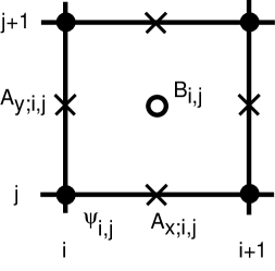
Fig. 1: Computational cell with evaluation points for $\psi$, $A_{x}$, and $A_{y}$.

The values of the link variables and the supercurrent are computed from the expressions

$$U_{x;i,j}={\rm e}^{-i\kappa^{-1}h_{x}A_{x;i,j}} \quad U_{y;i,j}={\rm e}^{-i\kappa^{-1}h_{y}A_{y;i,j}},$$ , (21)

$$J_{x;i,j}=\frac{1}{\kappa h_{x}}{\rm Im}\left[\psi_{i,j}^{*}U_{x;i,j}\psi_{i+1,j}\right] \quad J_{y;i,j}=\frac{1}{\kappa h_{y}}{\rm Im}\left[\psi_{i,j}^{*}U_{y;i,j}\psi_{i,j+1}\right].$$ , (22)

The discretized TDGL equations are

$$\frac{{\rm d}\psi_{i,j}}{{\rm d}t} = \left(L_{xx}(U_{x;\cdot,j})\psi_{\cdot,j}\right)_{i}+\left(L_{yy}(U_{y;i,\cdot})\psi_{i,\cdot}\right)_{j}+N\left(\psi_{i,j}\right),\quad(i,j)\in\mbox{Sc},$$ (23)

$$\sigma\frac{{\rm d}A_{x;i,j}}{{\rm d}t} = \left(D_{yy}A_{x;i,\cdot}\right)_{j}-\left(D_{yx}A_{y;\cdot,\cdot}\right)_{i,j}+J_{x;i,j},\quad(i,j)\in\mbox{Sc}\cup\mbox{Bl},$$ (24)

$$\sigma\frac{{\rm d}A_{y;i,j}}{{\rm d}t} = \left(D_{xx}A_{y;\cdot,j}\right)_{i}-\left(D_{xy}A_{x;\cdot,\cdot}\right)_{i,j}+J_{y;i,j}.\quad(i,j)\in\mbox{Sc}\cup\mbox{Bl},$$ (25)

where

$$\hskip 40.00006pt\left(L_{xx}(U_{x;\cdot,j})\psi_{\cdot,j}\right)_{i} = h_{x}^{-2}\left[U_{x;i,j}\psi_{i+1,j}-2\psi_{i,j}+U_{x;i-1,j}^{*}\psi_{i-1,j}\right],$$ (26)

$$\left(L_{yy}(U_{y;i,\cdot})\psi_{i,\cdot}\right)_{j} = h_{y}^{-2}\left[U_{y;i,j}\psi_{i,j+1}-2\psi_{i,j}+U_{y;i,j-1}^{*}\psi_{i,j-1}\right],$$ (27)

$$N\left(\psi_{i,j}\right) = \tau_{i,j}\psi_{i,j}-|\psi_{i,j}|^{2}\psi_{i,j},$$ (28)

$$\left(D_{yy}A_{x;i,\cdot}\right)_{j} = h_{y}^{-2}\left[A_{x;i,j+1}-2A_{x;i,j}+A_{x;i,j-1}\right],$$ (29)

$$\left(D_{xx}A_{y;\cdot,j}\right)_{i} = h_{x}^{-2}\left[A_{y;i+1,j}-2A_{y;i,j}+A_{y;i-1,j}\right],$$ (30)

$$\left(D_{yx}A_{y;\cdot,\cdot}\right)_{i,j} = h_{x}^{-1}h_{y}^{-1}\left[\left(A_{y;i+1,j}-A_{y;i,j}\right)-\left(A_{y;i+1,j-1}-A_{y;i,j-1}\right)\right],$$ (31)

$$\left(D_{xy}A_{x;\cdot,\cdot}\right)_{i,j} = h_{x}^{-1}h_{y}^{-1}\left[\left(A_{x;i,j+1}-A_{x;i,j}\right)-\left(A_{x;i-1,j+1}-A_{x;i-1,j}\right)\right].$$ (32)

The interface conditions are

$$\psi_{n_{sx}-1,j}=U_{x;n_{sx}-1,j}\psi_{n_{sx},j},\;\psi_{n_{ex}+1,j}=U^{*}_{x;n_{ex},j}\psi_{n_{ex},j},\;j=1,\ldots\,,n_{y}.$$ (33)

At the outer boundary, $B$ is given,

$$B_{0,j}=H_{L_{j}},\;B_{n_{x},j}=H_{R_{j}},\;j=1,\ldots\,,n_{y}.$$ (34)

The resulting approximation is second-order accurate [8].

3 Time Integration

We now address the integration of Eqs. (23)–(25). The first equation, which controls the evolution of $\psi$, involves the second-order linear finite-difference operators $L_{xx}$ and $L_{yy}$, whose coefficients depend on $A_{x}$ and $A_{y}$, and the local nonlinear operator $N$, which involves neither $A_{x}$ nor $A_{y}$. Each of the other two equations, which control the evolution of $A_{x}$ and $A_{y}$ respectively, involves likewise a second-order linear finite-difference operator, but with constant coefficients, and the nonlinear supercurrent operator, which involves $\psi$, $A_{x}$, and $A_{y}$. The following algorithms are distinguished by whether the various operators are treated explicitly or implicitly.

3.1 Fully Explicit Integration

Algorithm I uses a fully explicit forward Euler time-marching procedure for $\psi$, $A_{x}$, and $A_{y}$. Starting from an initial triple $(\psi^{0},A_{x}^{0},A_{y}^{0})$, we solve for $n=0,1,\ldots\,$,

$$\frac{\psi^{n+1}_{i,j}-\psi^{n}_{i,j}}{\Delta t} = \left(L_{xx}(U^{n}_{x;\cdot,j})\psi^{n}_{\cdot,j}\right)_{i}+\left(L_{yy}(U^{n}_{y;i,\cdot})\psi^{n}_{i,\cdot}\right)_{j}+N\left(\psi^{n}_{i,j}\right),\quad(i,j)\in\mbox{Sc},$$ (35)

$$\sigma\frac{A^{n+1}_{x;i,j}-A^{n}_{x;i,j}}{\Delta t} = \left(D_{yy}A^{n}_{x;i,\cdot}\right)_{j}-\left(D_{yx}A^{n}_{y;\cdot,\cdot}\right)_{i,j}+J^{n}_{x;i,j},\quad(i,j)\in\mbox{Sc}\cup\mbox{Bl},$$ (36)

$$\sigma\frac{A^{n+1}_{y;i,j}-A^{n}_{y;i,j}}{\Delta t} = \left(D_{xx}A^{n}_{y;\cdot,j}\right)_{i}-\left(D_{xy}A^{n}_{x;\cdot,\cdot}\right)_{i,j}+J^{n}_{y;i,j}.\quad(i,j)\in\mbox{Sc}\cup\mbox{Bl},$$ (37)

where $J^{n}$ is defined in terms of $\psi^{n}$, $A^{n}_{x}$, and $A^{n}_{y}$ in the obvious way. The initial triple is usually chosen so the superconductor is in the Meissner state, with a seed present to trigger the transition to the vortex state.

Algorithm I has been described in [8]. It has been implemented in a distributed-memory multiprocessor environment (IBM SP2); the transformations necessary to achieve the parallelism have been described in [9]. The code uses the Message Passing Interface (MPI) standard [10] as implemented in the MPICH software library [11] for domain decomposition, interprocessor communication, and file I/O. The code has been used extensively to study vortex dynamics in superconducting media [5, 6, 7]. The underlying algorithm provides highly accurate solutions but requires a significant number of time steps for equilibration. For stability reasons, the time step $\Delta t$ cannot exceed 0.0025.

3.2 Semi-Implicit Integration

Algorithm II is generated by an implicit treatment of the second-order linear finite-difference operators $D_{yy}$ and $D_{xx}$ in the equations for $A_{x}$ and $A_{y}$, respectively,

$$\frac{\psi^{n+1}_{i,j}-\psi^{n}_{i,j}}{\Delta t} = \left(L_{xx}(U^{n}_{x;\cdot,j})\psi^{n}_{\cdot,j}\right)_{i}+\left(L_{yy}(U^{n}_{y;i,\cdot})\psi^{n}_{i,\cdot}\right)_{j}+N\left(\psi^{n}_{i,j}\right),\quad(i,j)\in\mbox{Sc},$$ (38)

$$\sigma\frac{A^{n+1}_{x;i,j}-A^{n}_{x;i,j}}{\Delta t} = \left(D_{yy}A^{n+1}_{x;i,\cdot}\right)_{j}-\left(D_{yx}A^{n}_{y;\cdot,\cdot}\right)_{i,j}+J^{n}_{x;i,j},\quad(i,j)\in\mbox{Sc}\cup\mbox{Bl},$$ (39)

$$\sigma\frac{A^{n+1}_{y;i,j}-A^{n}_{y;i,j}}{\Delta t} = \left(D_{xx}A^{n+1}_{y;\cdot,j}\right)_{i}-\left(D_{xy}A^{n}_{x;\cdot,\cdot}\right)_{i,j}+J^{n}_{y;i,j}.\quad(i,j)\in\mbox{Sc}\cup\mbox{Bl}.$$ (40)

Equations (39) and (40) lead to two linear systems of equations,

$$\left(I-\frac{\Delta t}{\sigma}D_{yy}\right)A^{n+1}_{x;i} = F_{i}(\psi^{n},A^{n}_{x},A^{n}_{y}),\quad i=1,\ldots\,,n_{x}-1,$$ (41)

$$\left(I-\frac{\Delta t}{\sigma}D_{xx}\right)A^{n+1}_{y;j} = G_{j}(\psi^{n},A^{n}_{x},A^{n}_{y}),\quad j=1,\ldots\,,n_{y},$$ (42)

for the vectors of unknowns $A_{x;i}=\{A_{x;i,j}:j=1,\ldots\,,n_{y}\}$ and $A_{y;j}=\{A_{y;i,j}:i=1,\ldots\,,n_{x}-1\}$. The matrix $D_{yy}$ has dimension $n_{y}\times n_{y}$ and is periodic tridiagonal with elements $-h_{y}^{-2},2h_{y}^{-2},-h_{y}^{-2}$; the matrix $D_{xx}$ has dimension $(n_{x}-1)\times(n_{x}-1)$ and is tridiagonal with elements $-h_{x}^{-2},2h_{x}^{-2},-h_{x}^{-2}$, (except along the edges, because of the boundary conditions). Both matrices are independent of $i$ and $j$. Furthermore, if the boundary conditions are time independent, they are constant throughout the time-stepping process. Hence, the coefficient matrices in Eqs. (41) and (42) need to be factored only once; in fact, the factorization can be done in the preprocessing stage and the factors can be stored.

In a parallel processing environment, the coefficient matrices extend over several processors, so Eqs. (41) and (42) are broken up in blocks corresponding to the manner in which the computational mesh is distributed among the processor set. We first solve the equations within each processor (inner iterations) and then couple the solutions across processor boundaries (outer iterations). Hence, we deal with interprocessor coupling in an iterative fashion. Two to three inner iterations usually suffice to reach a desired tolerance for convergence. After each inner iteration, each processor shares boundary data with its neighbors through MPI calls.

3.3 Implicit Integration

Algorithm III combines the semi-implicit treatment of $A_{x}$ and $A_{y}$ with an implicit treatment of the order parameter,

$$\frac{\psi^{n+1}_{i,j}-\psi^{n}_{i,j}}{\Delta t} = \left(L_{xx}(U^{n}_{x;\cdot,j})\psi^{n+1}_{\cdot,j}\right)_{i}+\left(L_{yy}(U^{n}_{y;i,\cdot})\psi^{n+1}_{i,\cdot}\right)_{j}+N\left(\psi^{n}_{i,j}\right),\quad(i,j)\in\mbox{Sc},$$ (43)

$$\sigma\frac{A^{n+1}_{x;i,j}-A^{n}_{x;i,j}}{\Delta t} = \left(D_{yy}A^{n+1}_{x;i,\cdot}\right)_{j}-\left(D_{yx}A^{n}_{y;\cdot,\cdot}\right)_{i,j}+J^{n}_{x;i,j},\quad(i,j)\in\mbox{Sc}\cup\mbox{Bl},$$ (44)

$$\sigma\frac{A^{n+1}_{y;i,j}-A^{n}_{y;i,j}}{\Delta t} = \left(D_{xx}A^{n+1}_{y;\cdot,j}\right)_{i}-\left(D_{xy}A^{n}_{x;\cdot,\cdot}\right)_{i,j}+J^{n}_{y;i,j}.\quad(i,j)\in\mbox{Sc}\cup\mbox{Bl}.$$ (45)

The second and third equation are solved as in the semi-implicit algorithm of the preceding section. The first equation is solved by a method similar to the method of Douglas and Gunn [12] for the Laplacian.

We begin by transforming Eq. (43) into an equation for the correction matrix $\phi^{n+1}=\psi^{n+1}-\psi^{n}$. The equation has the general form

$$\left(I-\Delta t(L_{xx}+L_{yy})\right)\phi^{n+1}=F(\psi^{n},A_{x}^{n},A_{y}^{n}).$$ (46)

If $\Delta t$ is sufficiently small, we may replace the operator in the left member by an approximate factorization,

$$\left(I-\Delta t(L_{xx}+L_{yy})\right)\approx\left(I-\Delta tL_{xx}\right)\left(I-\Delta tL_{yy}\right),$$ (47)

and consider, instead of Eq. (46),

$$\left(I-\Delta tL_{xx}\right)\left(I-\Delta tL_{yy}\right)\phi^{n+1}=F(\psi^{n},A_{x}^{n},A_{y}^{n}).$$ (48)

This equation can be solved in two steps,

$$\left(I-\Delta tL_{xx}\right)\varphi = F,$$ (49)

$$\left(I-\Delta tL_{yy}\right)\phi^{n+1} = \varphi.$$ (50)

The conditions (33), which must be satisfied at the interface between the superconductor and the blanket material, require some care. If we impose the conditions at every time step, then

$$\phi^{n+1}_{n_{sx}-1,j} = U^{n+1}_{x;n_{sx}-1,j}\phi^{n+1}_{n_{sx},j}+\left[U^{n+1}_{x;n_{sx}-1,j}-U^{n}_{x;n_{sx}-1,j}\right]\psi^{n}_{n_{sx},j},$$

$$\phi^{n+1}_{n_{ex}+1,j} = \left(U^{n+1}_{x;n_{ex},j}\right)^{*}\phi^{n+1}_{n_{ex},j}+\left[\left(U^{n+1}_{x;n_{ex},j}\right)^{*}-\left(U^{n}_{x;n_{sx}-1,j}\right)^{*}\right]\psi^{n}_{n_{sx},j},$$

for $j=1,\ldots\,,n_{y}$. These conditions couple the correction $\phi$ to the update of $A_{x}$. To eliminate this coupling, we solve Eq. (46) subject to the reduced interface conditions

$$\phi^{n+1}_{n_{sx}-1,j} = U^{n+1}_{x;n_{sx}-1,j}\phi^{n+1}_{n_{sx},j},\;j=1,\ldots\,,n_{y},$$ (51)

$$\phi^{n+1}_{n_{ex}+1,j} = \left(U^{n+1}_{x;n_{ex},j}\right)^{*}\phi^{n+1}_{n_{ex},j},\;j=1,\ldots\,,n_{y}.$$ (52)

When Eq. (46) is replaced by Eq. (48), these conditions are inherited by the system (49).

3.4 Fully Implicit Integration

Algorithm IV uses a fully implicit integration procedure for the order parameter,

$$\frac{\psi^{n+1}_{i,j}-\psi^{n}_{i,j}}{\Delta t} = \left(L_{xx}(U^{n}_{x;\cdot,j})\psi^{n+1}_{\cdot,j}\right)_{i}+\left(L_{yy}(U^{n}_{y;i,\cdot})\psi^{n+1}_{i,\cdot}\right)_{j}+N\left(\psi^{n+1}_{i,j}\right),\quad(i,j)\in\mbox{Sc},$$ (53)

$$\sigma\frac{A^{n+1}_{x;i,j}-A^{n}_{x;i,j}}{\Delta t} = \left(D_{yy}A^{n+1}_{x;i,\cdot}\right)_{j}-\left(D_{yx}A^{n}_{y;\cdot,\cdot}\right)_{i,j}+J^{n}_{x;i,j},\quad(i,j)\in\mbox{Sc}\cup\mbox{Bl},$$ (54)

$$\sigma\frac{A^{n+1}_{y;i,j}-A^{n}_{y;i,j}}{\Delta t} = \left(D_{xx}A^{n+1}_{y;\cdot,j}\right)_{i}-\left(D_{xy}A^{n}_{x;\cdot,\cdot}\right)_{i,j}+J^{n}_{y;i,j}.\quad(i,j)\in\mbox{Sc}\cup\mbox{Bl}.$$ (55)

The new element here is the term $N\left(\psi^{n+1}_{i,j}\right)$ in the first equation.

The second and third equations are solved again as in the semi-implicit algorithm. The first equation is solved by a slight modification of the method used in the implicit algorithm of the preceding section, The modification is brought about by the approximation

$$N\left(\psi^{n+1}\right)=\tau\psi^{n+1}-|\psi^{n+1}|^{2}\psi^{n+1}\approx\frac{1}{\Delta t}\left(S\left(\psi^{n}\right)-\psi^{n}\right),$$ (56)

where $S$ is a nonlinear map,

$$S(\psi)=\frac{\tau^{1/2}\psi}{\left[|\psi|^{2}+(\tau-|\psi|^{2})\exp(-2\tau\Delta t)\right]^{1/2}}.$$ (57)

(This approximation is explained in the remark below.) Equation (53) is again of the form (46), but with a different right-hand side,

$$(I-\Delta t(L_{xx}+L_{yy}))\phi^{n+1}=G(\psi^{n},A_{x}^{n},A_{y}^{n}).$$ (58)

The difference is that, where $F$ in Eq. (46) contains a term $(\Delta t)N\left(\psi^{n}\right)$, $G$ in Eq. (58) contains the more complicated term $S\left(\psi^{n}\right)-\psi^{n}$.

Remark

The approximation (56) is suggested by semigroup theory. Symbolically,

$$N(\psi)=\lim_{\Delta t\to 0}\frac{S(\Delta t)\psi-\psi}{\Delta t}.$$ (59)

To find an expression for the “semigroup” $S$, we start from the continuous TDGL equations (6)–(8) (zero-electric potential gauge, $\Phi=0$), using the polar representation $\psi=|\psi|{\rm e}^{i\phi}$,

$$\partial_{t}|\psi| = \Delta|\psi|-|\psi||\nabla\phi-\kappa^{-1}\mbox{$\mathbf{A}$}|^{2}+\tau|\psi|-|\psi|^{3},$$ (60)

$$|\psi|\partial_{t}\phi = 2(\nabla|\psi|)\cdot(\nabla\phi-\kappa^{-1}\mbox{$\mathbf{A}$})+|\psi|\nabla\cdot(\nabla\phi-\kappa^{-1}\mbox{$\mathbf{A}$}),$$ (61)

$$\sigma\partial_{t}\mbox{$\mathbf{A}$} = -\nabla\times\nabla\times\mbox{$\mathbf{A}$}+\kappa^{-1}|\psi|^{2}(\nabla\phi-\kappa^{-1}\mbox{$\mathbf{A}$}).$$ (62)

At this point, we are interested in the effect of the nonlinear term $|\psi|^{3}$ on the dynamics. To highlight this effect, we concentrate on the time evolution of the scalar $u=|\psi|$ and the vector $v=\nabla\phi-\kappa^{-1}\mbox{$\mathbf{A}$}$. (In physical terms, $u^{2}$ is the density of superconducting charge carriers, while $u^{2}v$ is $\kappa$ times the supercurrent density.) Ignoring their spatial variations, we have a dynamical system,

$$u^{\prime} = -u|v|^{2}+\tau u-u^{3},$$ (63)

$$v^{\prime} = -\varepsilon u^{2}v,$$ (64)

where ^′ denotes differentiation with respect to $t$, and $\varepsilon=(\kappa^{2}\sigma)^{-1}$. This system yields a pair of ordinary differential equations for the scalars $x=u^{2}$ and $y=|v|^{2}$,

$$x^{\prime} = 2x(\tau-x-y),$$ (65)

$$y^{\prime} = -2\varepsilon xy.$$ (66)

If $\kappa$ is large, $\varepsilon$ is small, and the dynamics are readily analyzed. To leading order, $y$ is constant; $y=0$ is the only meaningful choice. (Recall that $xy^{1/2}$ is $\kappa$ times the magnitude of the supercurrent density.) Then the dynamics of $x$ are given by

$$x^{\prime}=2x(\tau-x).$$ (67)

We integrate this equation from $t=t_{n}$ to $t$,

$$x(t)=\frac{\tau x(t_{n})}{x(t_{n})+(\tau-x(t_{n}))\exp(-2\tau(t-t_{n}))}.$$ (68)

In particular,

$$x(t_{n+1})=\frac{\tau x(t_{n})}{x(t_{n})+(\tau-x(t_{n}))\exp(-2\tau\Delta t)},$$ (69)

where $\Delta t=t_{n+1}-t_{n}$. Since $x(t_{n})=|\psi^{n}|^{1/2}$ and $x(t_{n+1})=|\psi^{n+1}|^{1/2}$, it follows that

$$|\psi^{n+1}|=\frac{\tau^{1/2}|\psi^{n}|}{[|\psi^{n}|^{2}+(\tau-|\psi^{n}|^{2})\exp(-2\tau\Delta t)]^{1/2}}.$$ (70)

The phase $\phi$ of $\psi$ is constant in time. If we multiply both sides by ${\rm e}^{i\phi}$, we obtain the expression (57) for the “semigroup” $S$.

4 Evaluation

We now present the results of several experiments, where the algorithms described in the preceding section were applied to a benchmark problem.

4.1 Benchmark Problem

The benchmark problem adopted for this investigation was the equilibration of a vortex configuration in a superconductor (Ginzburg-Landau parameter $\kappa=16$) embedded in a thin insulator (air), where the entire system was periodic in the direction of the free surfaces ($y$).

The superconductor measured $128\xi$ in the transverse ($x$) direction. The thickness of the insulating layer on either side was taken to be $2\xi$, so the total width of the system was $132\xi$. The period in the $y$ direction was taken to be $192\xi$, so the entire configuration measured $132\xi\times 192\xi$.

The computational grid was uniform, with a mesh width $h_{x}=h_{y}={\textstyle{1\over 2}}\xi$. The periodic boundary conditions in the $y$ direction were handled through ghost points, so the computational grid had $264\times 386$ vertices. The index sets for the superconductor and blanket (see Eqs. (16) and (17)) were

Sc $$= \{(i,j):i=5,\ldots\,,260,\,j=1,\ldots\,,386\},$$ (71)

Bl $$= \{(i,j):i=1,\ldots\,,4,261,\ldots\,,264,\,\,j=1,\ldots\,,386\}.$$ (72)

The applied field was uniform in $y$ and equally strong on the left and right side of the system,

$$H_{L}=H_{R}=H=0.5.$$ (73)

(Units of $H$ are $H_{c}\surd 2$, so $H\approx 0.707\ldots H_{c}$). As there is no transport current in the system, the solution of the TDGL equations tends to an equilibrium state.

4.2 Benchmark Solution

First, preliminary runs were made to determine, for each algorithm, the optimal number of processors in a multiprocessing environment. Figure 2 shows the elapsed (wall clock) time for 50 time steps against the number of processors on the IBM SP2.

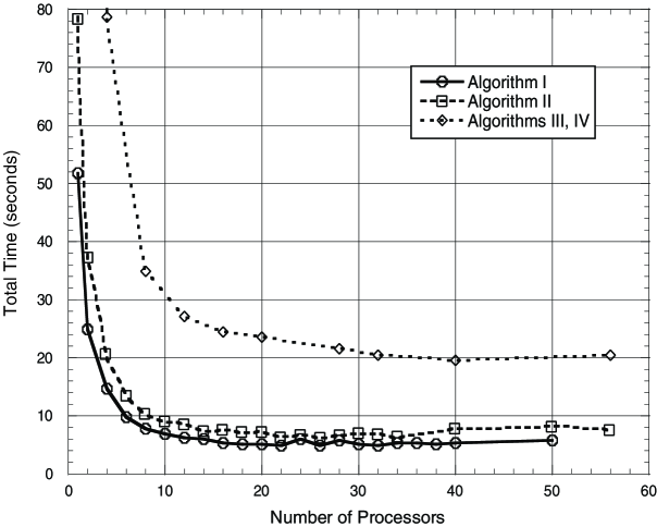
Fig. 2: Elapsed time for 50 time steps as a function of the number of processors.

Each algorithm showed a saturation around 16 processors, beyond which any improvement became marginal. All problems were subsequently run on 16 processors.

Next, the fully explicit Algorithm I was used to establish a benchmark equilibrium configuration. Equations (35)–(37) were integrated with a time step $\Delta t=0.0025$ (units of $\xi^{2}/D$), the maximal value for which the algorithm remained stable. The evolution of the vortex configuration was followed by monitoring the number of vortices and their positions. Equilibrium was reached after 10,000,000 time steps, when the number of vortices remained constant and the vortex positions varied less than $1.0\times 10^{-6}$ (units of $\xi$). The equilibrium vortex configuration had 116 vortices arranged in a hexagonal pattern; see Fig. 3.

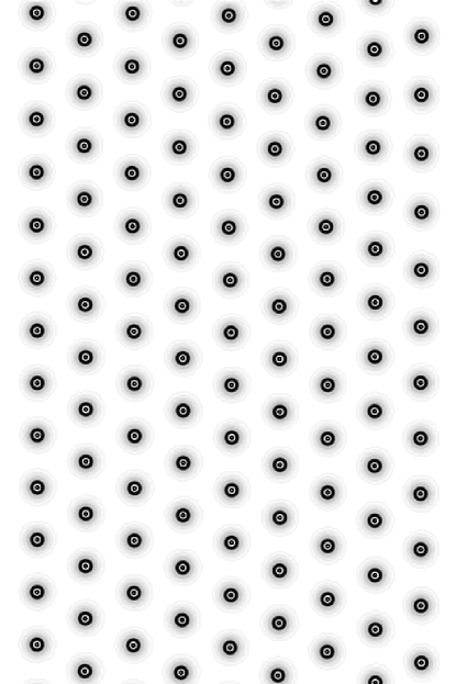
Fig. 3: Equilibrium vortex configuration for the benchmark problem.

The elapsed time for the entire computation was 50.81 hours. The elapsed time per time step (0.018 seconds) is a measure for the computational cost of Algorithm I.

4.3 Evaluation of Algorithms II–IV

Once the benchmark solution was in place, each of the remaining algorithms (II–IV) was evaluated for stability, accuracy, and computational cost.

The stability limit was found by gradually increasing the time step and integrating until equilibrium. Above the stability limit, the algorithm failed because of arithmetic divergences. Equilibrium was defined by the same criteria as for the benchmark solution: no change in the number of vortices and a variation in the vortex positions of less than $1.0\times 10^{-6}$. The results are given in Table 1; $\Delta t$ is the time step at the stability limit (units of $\xi^{2}/D$), $N$ the number of time steps needed to reach equilibrium, $T$ the elapsed (wall clock) time (in hours) needed to compute the equilibrium configuration, and $C$ the cost (in seconds per time step, $C=3600T/N$).

Because each algorithm defines its own path through phase space, one cannot expect to find identical equilibrium configurations nor equilibrium configurations that are exactly the same as the benchmark. The equilibrium vortex configurations for the four algorithms were indeed different, albeit slightly. To measure the differences quantitatively, we computed the following three parameters: (1) the number of vortices in the superconducting region, (2) the mean bond length joining neighboring pairs of vortices, and (3) the mean bond angle subtended by neighboring bonds throughout the vortex lattice. In all cases, the number of vortices was the same (116); the mean bond length varied less than $1.0\times 10^{-3}\xi$, and the mean bond angle varied by less than $1.0\times 10^{-3}$ radians. Within these tolerances, the equilibrium vortex configurations were the same.

Table 1: Performance data for Algorithms I–IV.

	$\Delta t$	$N$	$C$	$T$
Algorithm
I	0.0025	10,000,000	0.018	50.81
II	0.0500	500,000	0.103	14.32
III	0.1000	250,000	0.232	16.11
IV	0.1900	131,580	0.233	8.41

Finally, we evaluated the fully implicit Algorithm IV from the point of view of parallelism. From the benchmark problem we derived two more problems by twice doubling the size of the system in each direction, while keeping the mesh width the same (${\textstyle{1\over 2}}\xi$). The resulting computational grid had $528\times 772$ vertices for the intermediate problem and $1056\times 1544$ vertices for the largest problem. Speedup was defined as the ratio of the wall clock time (exclusive of I/O) to reach equilibrium on $p$ processors divided by the time to reach equilibrium on a single processor for the smallest and intermediate problem, or twice the time to reach equilibrium on two processors for the largest problem. (The largest problem did not fit on a single processor.) The results are given in Fig. 4.

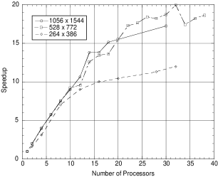
Fig. 4: Computational cell with evaluation points for $\psi$, $A_{x}$, and $A_{y}$.

The curve for the benchmark problem was obtained as an average over many runs; the data for the intermediate and largest problem were obtained from single runs, hence they are less smooth. The speedup is clearly linear when the number of processors is small; it becomes sublinear at about 12 processors for the smallest problem, 14 processors for the intermediate problem, and 18 processors for the largest problem.

5 Conclusions

The results of the investigation lead to the following conclusions.

(1) One can increase the time step $\Delta t$ nearly 80-fold, without losing stability, by going from the fully explicit Algorithm I to the fully implicit Algorithm IV.

(2) As one goes to the fully implicit Algorithm IV, the complexity of the matrix calculations and, hence, the cost $C$ of a single time step increase.

(3) The increase in the cost $C$ per time step is more than offset by the increase in the size of the time step $\Delta t$. In fact, the wall clock time needed to compute the same equilibrium state with the fully implicit Algorithm IV is one-sixth of the wall clock time for the fully explicit Algorithm I.

(4) The (physical) time to reach equilibrium—that is, $N\Delta t$, the number of time steps needed to reach equilibrium times the step size—is (approximately) the same for all algorithms, namely, 25,000 (units of $\xi^{2}/D$).

(5) The fully implicit Algorithm IV displays linear speedup in a multiprocessing environment. The speedup curves show sublinear behavior when the number of processors is large.

References

- [1] V. L. Ginzburg and L. D. Landau, On the theory of superconductivity, Zh. Eksp. Teor. Fiz. (USSR) 20 (1950,) 1064–1082; Engl. transl. in D. ter Haar, L. D. Landau; Men of Physics, Vol. I, Pergamon Press, Oxford, 1965, pp. 138–167 .
- [2] M. Tinkham, Introduction to Superconductivity (2nd edition), McGraw-Hill, Inc., New York, 1996.
- [3] A. Schmid, A time dependent Ginzburg–Landau equation and its application to a problem of resistivity in the mixed state, Phys. kondens. Materie, 5 (1966), 302–317.
- [4] L. P. Gor’kov and G. M. Éliashberg, Generalizations of the Ginzburg–Landau equations for non-stationary problems in the case of alloys with paramagnetic impurities, Zh. Eksp. Teor. Fiz., 54 (1968), 612–626; Soviet Phys.—JETP, 27 (1968), 328–334.
- [5] D. W. Braun et al., Structure of a moving vortex lattice, Phys. Rev. Lett., 76 (1996), 831–834.
- [6] G. W. Crabtree et al., Time-dependent Ginzburg-Landau simulations of vortex guidance by twin boundaries, Physica C, 263 (1996), 401–408.
- [7] G. C. Crabtree et al., Vortex motion through defects, Preprint ANL/MCS-P764-0699, Argonne National Laboratory, Argonne, Ill., 1999.
- [8] W. D. Gropp et al., Numerical simulations of vortex dynamics in type-II superconductors, J. Comp. Phys., 123 (1996), 254–266.
- [9] N. Galbreath et al., Parallel solution of the three-dimensional, time-dependent Ginzburg-Landau equation, Proc. Sixth SIAM Conference on Parallel Processing for Scientific Computing, R. F. Sincovec, D. E. Keyes, M. R. Leuze, L. R. Petzold, and D. A. Reed (eds.), SIAM, Philadelphia, 1993, pp. 160-164.
- [10] J. Dongarra et al., MPI–The Complete Reference, Vols. I & II, MIT Press, Cambridge, Mass., 1998.
- [11] W. Gropp et al., A High-Performance, Portable Implementation of the MPI Message Passing Interface Standard, Technical Report ANL/MCS-P567-0296, Argonne National Laboratory, Argonne, Ill., 1996.
- [12] J. Douglas and J. E. Gunn, A general formulation of alternating direction methods—Part I: Parabolic and hyperbolic problems, Numerische Mathematik, 6 (1964), 428–453.