Quadratic Control Lyapunov Functions for Bilinear Systems

Abstract

In this paper the existence of a quadratic control Lyapunov function for bilinear systems is considered. The existence of a control Lyapunov function ensures the existence of a control law which ensures the global asymptotic stability of the closed loop control system. In this paper we will derive conditions for the existence of a control Lyapunov function for bilinear systems. These conditions will be derived for the whole class of two dimensional bilinear systems with one control input. This will lead to a simple flow diagram representation for the controller design for bilinear systems using a quadratic control Lyapunov function. The controller design itself is carried out using Sontag’s universal control law [1] to obtain an asymptotically stable closed loop system. The Gutman control law [2] which, however, only ensures practical stability of the closed loop system but which is considerably simpler than Sontag’s control law will also be considered. An example will conclude the paper.

1 Introduction

In this paper bilinear systems (BLS) given by the state space representation

$$\dot{x}(t)=Ax(t)+\sum_{i=1}^{m}(N_{i}x(t)+b_{i})u_{i}(t)\,,\quad x(0)=x^{0}$$ (1)

are in the focus of interest. In (1) the symbol $x(t)\in R^{n}$ represents the state vector and $u(t)\in R^{m}$ represents the vector of control inputs. The matrices $A$ and $N_{i},i=1,\ldots,m$ are real $n\times n$ matrices while the vectors $b_{i},i=1,\ldots,m$ are real $n$-dimensional vectors. Applying the results from [1, 3, 4] to the class of BLS it turns out that $V(x)=x^{T}Px$ with a symmetric and positive definite $n\times n$ matrix $P$ is a control Lyapunov function (CLF) for (1) if and only if

$$Y(x):=x^{T}(A^{T}P+PA)x<0\quad\forall\,x\in M:=\left\{x\in R^{n}\left|\,\,x\neq 0\,\,,\,\,\sum_{i=1}^{m}((N_{i}x+b_{i})^{T}Px)^{2}=0\right.\right\}$$ (2)

is valid. If $V(x)$ is a CLF the control law derived by Artstein and Sontag [1, 3] ensures the global asymptotic stability of the closed loop system. It should be mentioned that (2) is identical with the design conditions derived by Gutman [2] and Mohler [5] for the controller design for BLS. However, in general the condition (2) is extremely hard to check and to fulfill.

In a numerical study, where a large set of bilinear systems has been considered we were in all cases unable to compute a matrix $P$ such that (2) is fulfilled. This numerical problem was the main motivation to analyse the design conditions for a special class of bilinear system, namely, two dimensional single input bilinear systems given by the state space representation

$$\dot{x}(t)=A\,x(t)+(Nx(t)+b)u(t),\,\,x(0)=x^{0}$$ (3)

where the two dimensional state vector is represented by $x(t)=(x_{1}(t),x_{2}(t))^{T}$ and the input $u(t)$ is a scalar function of time. The matrices $A$ and $N$ are real $2\times 2$ matrices and $b$ is a two dimensional vector. For this class of bilinear systems the computation of a positive definite and symmetric $2\times 2$ matrix $P=P^{T}>0$ for which

$$Y(x)<0\quad\forall x\in M$$ (4)

is satisfied will be carried out. In this special case the above definitions for $Y(x)$ and $M$ are simplified to

$$Y(x) = x^{T}(A^{T}P+P\,A)x=x^{T}A_{p}x\,,$$ (5)

$$M = \{x\mid x\neq 0,\quad(N\,x+b)^{T}P\,x=0\}=\{x\mid x\neq 0,\quad x^{T}N_{p}x+2x^{T}P\,b=0\}$$ (6)

where the abbreviations

$$A_{p} := A^{T}P+P\,A\,,$$ (7)

$$N_{p} := N^{T}P+P\,N$$ (8)

for the corresponding symmetric and real $2\times 2$ matrices have been introduced. The set $M$ defines a conic section in the $x$-plane whereby the shape of this conic section depends on the eigenvalues of $N_{p}$. For the analysis of the controller design a case study with respect to $N_{p}$ will be done. Especially positive definite, negative definite, semi definite and indefinite matrices $N_{p}$ and the case $N_{p}=0$ have to be considered. In the following section a necessary condition for $P$ will be derived from (4). The third section contains a detailed discussion of the positive definite case $N_{p}>0$. The extension to the remaining cases will be outlined and the results for all cases are presented as a flow diagram. The paper ends with an example and the conclusions. It should be mentioned that most of the computations were performed using the computer algebra system MAPLE [6].

2 Necessary Condition

The main goal in this section is to derive a necessary condition for $P$ from the design condition (4). Because of $Y(0)=0$ the function $Y(x)$ has to have a local maximum at $x=0$ with respect to the constraint $x\in M$ because otherwise the condition (4) is violated in a vincinity of $x=0$. First we analyse if $Y(x)$ has a local extremum if the constraint $x^{T}N_{p}x+2x^{T}P\,b=0$ which defines $M$ is active. To answer this, we define the Lagrange function $L(x,\lambda)=x^{T}A_{p}x+\lambda(x^{T}N_{p}x+2x^{T}Pb)$ using the Lagrange multiplicator $\lambda$. The necessary conditions for a local extremum using the partial derivatives are calculated as

$$\frac{\partial L}{\partial x}=2(A_{p}+\lambda N_{p})x+2\lambda Pb\stackrel{{\scriptstyle!}}{{=}}0,\quad\frac{\partial L}{\partial\lambda}=x^{T}N_{p}x+2x^{T}Pb\stackrel{{\scriptstyle!}}{{=}}0.$$ (9)

It is easily verified that $\lambda=0$, $x=0$ is a solution of (9) and consequently $x=0$ is a local extremal point of $Y(x)$ under the constraint $x^{T}N_{p}x+2x^{T}P\,b=0$. As discussed above $x=0$ is required to be a local maximum. A necessary and sufficient condition [7] for this is, that

$$v^{T}(\frac{\partial^{2}}{\partial x^{2}}\{x^{T}A_{p}x\})v<0$$ (10)

is satisfied for all vectors $v$ that satisfy

$$v^{T}(\frac{\partial}{\partial x}\{x^{T}N_{p}x+2x^{T}P\,b\})\biggl{|}_{x=0}=0.$$ (11)

The needed partial derivatives are $\frac{\partial^{2}}{\partial x^{2}}\{x^{T}A_{p}x\}=2A_{p}$ and $\frac{\partial}{\partial x}\{x^{T}N_{p}x+2x^{T}P\,b\}\bigl{|}_{x=0}=2P\,b$. The desired vectors $v$ that are othogonal to $P\,b$ and therefore satisfy (11) are given by $v=\kappa J\,P\,b$ where $\kappa$ is a non zero scalar. In the two dimensional case the matrix $J$ is given by

$$J=\left(\begin{array}[]{cc}0&-1\\ 1&0\end{array}\right).$$ (12)

Now we are able to derive a condition that is equivalent to (10) and (11). It is given by $v^{T}A_{p}v=\kappa^{2}b^{T}PJ^{T}A_{p}JPb\,<0\,\,\forall\kappa\in R\backslash\{0\}$ which can be simplified to

$$b^{T}PJ^{T}A_{p}JPb<0$$ (13)

since $\kappa^{2}$ is positive. This condition will be simplified further. In the following we assume the pair $\{A,b\}$ to be completely controllable and choose $\{A,b\}$ in controller normal form such that

$$A=\left(\begin{array}[]{cc}0&1\\ -a_{0}&-a_{1}\end{array}\right),\,\,\,\,b=\left(\begin{array}[]{c}0\\ 1\end{array}\right)$$ (14)

where $a_{0}$ and $a_{1}$ are the coefficients of the characteristic polynomial of $A$. The positive definite and symmetric matrix $P$ is parameterized as

$$P=\left(\begin{array}[]{cc}1&p_{1}\\ p_{1}&p_{2}\end{array}\right)$$ (15)

where $p_{1}$ and $p_{2}$ are real variables and the fact that $P$ is determined up to a positive factor has been used to choose the $(1,1)$ element to 1. To ensure $P>0$ the variables $p_{1}$ and $p_{2}$ have to fulfill

$$p_{2}-p_{1}^{2}>0.$$ (16)

If we use (14) and (15) in (13) the condition (13) is equivalent to $p_{1}(p_{1}^{2}-p_{2})<0$. Using (16) this inequality reduces to

$$p_{1}>0$$ (17)

which is a necessary condition on $P$ and will be central for the following computations.

3 Sufficient Conditions

In this section we discuss the controller design conditions for the case of a positive definite matrix $N_{p}$. The main idea to analyse this situation is to carry out a linear state variable transformation to transform the set $M$ into a circle. After this transformation we parameterize $M$ and evaluate $Y(x)\,\,\forall x\in M$. In the following the transformed set $M$ and the transformed function $Y(x)$ will be called $M_{y}$ and $Y_{y}(y)$, respectively. It should be mentioned that temporarily $x=0$ will be allowed in $M$ for an easier calculation of the necessary transformation. After having carried out the transformation it will be indicated to which point $x=0$ has been transformed and the related transformed point will be omitted. For the positive definite matrix $N_{p}$ we carry out a cholesky decomposition [8] of the form $N_{p}=L^{T}L$ with a nonsingular matrix $L$ given by

$$L=\left(\begin{array}[]{cc}l_{1}&l_{2}\\ 0&l_{3}\end{array}\right)$$ (18)

where $l_{1}$ and $l_{3}$ are positive. With this matrix $L$ the above mentioned transformation is performed according to $x=L^{-1}(y+y_{0})\Leftrightarrow y=Lx-y_{0}$ where $y=(y_{1},y_{2})^{T}$ represents the new state vector and

$$y_{0}=-(L^{-1})^{T}Pb=\left(\begin{array}[]{c}-\frac{p_{1}}{l_{1}}\\ \frac{p_{1}l_{2}-p_{2}l_{1}}{l_{1}l_{3}}\end{array}\right)=\left(\begin{array}[]{c}y_{0,1}\\ y_{0,2}\end{array}\right)$$ (19)

is an appropriate choice. Substituting $x=L^{-1}(y+y_{0})$ into the equations which describe $M$ leads to the transformed set

$$M_{y}=\{y\in R^{2}\mid y_{1}^{2}+y_{2}^{2}=a\}\quad\mbox{with}\quad a=\frac{(p_{1}l_{2}-p_{2}l_{1})^{2}+(p_{1}l_{3})^{2}}{l_{1}^{2}l_{3}^{2}}>0$$ (20)

which describes a circle with radius $\sqrt{a}$ in the $y$-plane. This circle is now parameterized using rational functions, thus, the transformed set $M_{y}$ is represented by

$$M_{y}=\{y\mid y=\frac{\sqrt{a}}{1+t^{2}}\left(\begin{array}[]{c}1-t^{2}\\ \ 2t\end{array}\right),t\in R\}.$$ (21)

After having computed this representation of $M_{y}$ we are now able to evaluate $Y(x)\,\,\forall x\in M$, which has the same range of values as the transformed $Y_{y}(y)\,\,\forall y\in M_{y}$. We compute $Y_{y}(y)=Y(L^{-1}y+x_{0})$ and in order to evaluate $Y_{y}(y)\,\,\forall y\in M_{y}$ we further substitute

$$y=\frac{\sqrt{a}}{1+t^{2}}\left(\begin{array}[]{c}1-t^{2}\\ \ 2t\end{array}\right)$$ (22)

in $Y_{y}(y)$ and compute $Y_{y}(y)\,\forall y\in M_{y}$ as a rational function $\tilde{Y}_{y}(t)$ of the real variable $t$. The function $\tilde{Y}_{y}(t)$ is required to be negative for all real values of the variable $t$ to ensure that the design condition (4) holds. $\tilde{Y}_{y}(t)$ is a very complex rational function of the form $\tilde{Y}_{y}(t)=\frac{Z(t)}{N(t)}$, where numerator $Z(t)$ and denominator $N(t)$ are both polynomials of degree four in $t$. The denominator polynomial is computed as $N(t)=l_{1}^{4}l_{3}^{4}(1+t^{2})^{2}$ which is positive for all real values of $t$, thus, it can be ignored for the analysis of the sign of $\tilde{Y}_{y}(t)$. The numerator polynomial $Z(t)$ is factored as the product of two polynomials of degree two given by

$$Z(t)=(t-t_{0})^{2}\cdot P(t)\quad\mbox{with}\quad t_{0}=-\frac{-y_{0,2}}{\sqrt{a}+(-y_{0,1})}.$$ (23)

The special value $t_{0}$ corresponds to $x=0$ and because $x=0$ has to be excluded from $M$ we require $Z(t)<0\,\,\forall\,t\in R\backslash\{t_{0}\}$. For all values of $t\in R\backslash\{t_{0}\}$ the polynomial $(t-t_{0})^{2}$ is positive so it does not influence the sign of $\tilde{Y}_{y}(t)$. Thus, $P(t)$ is required to be negative for all real values of $t$ in order to satisfy the design condition (4). As mentioned above $P(t)$ is a polynomial of degree two of the form $P(t)=k_{2}t^{2}+k_{1}t+k_{0}$, where $k_{2}$, $k_{1}$ and $k_{0}$ are very complex expressions containing $l_{1}$, $l_{2}$, $l_{3}$, $p_{1}$, $p_{2}$, $a_{0}$ and $a_{1}$. If we require $P(t)<0$ for all $t\in R$ the following two cases have to be considered:

1. all coefficients $k_{2}$, $k_{1}$ and $k_{0}$ are non zero, thus,

   $$P(t^{*})<0\,\,\mbox{for some}\,\,t^{*}\,\,\mbox{and}\,\,k_{1}^{2}-4k_{0}k_{2}<0$$ (24)

   have to be fulfilled, in order to guarantee $P(t)<0$ for all real $t$;

2. the coefficients $k_{2}$ and $k_{1}$ are zero and therefore $P(t)=k_{0}$ is constant and $k_{0}<0$ has to be fulfilled.

These two cases will be discussed in the following. First case one is considered. If $t^{*}=t_{0}$ given by (23) is chosen, the conditions (24) are computed as

$$P(t_{0})=8l_{1}^{2}l_{3}^{2}p_{1}(p_{1}^{2}-p_{2}) < 0,$$ (25)

$$k_{1}^{2}-4k_{0}k_{2}=16\beta l_{1}^{2}l_{3}^{2}(\sqrt{\beta}+p_{1}l_{3})^{2}\cdot$$

$$\cdot(4p_{1}^{2}a_{0}+p_{1}^{2}a_{1}^{2}-2p_{1}p_{2}a_{0}a_{1}-2p_{1}a_{1}-2p_{2}a_{0}+p_{2}^{2}a_{0}^{2}+1) < 0$$ (26)

with $\beta=(p_{1}l_{2}-p_{2}l_{1})^{2}+(p_{1}l_{3})^{2}$. Considering the necessary conditions (16) and (17) one can easily conclude that condition (25) is satisfied. It is also obvious, that the factor $16\beta l_{1}^{2}l_{3}^{2}(\sqrt{\beta}+p_{1}l_{3})^{2}$ in (26) is positive and consequently,

$$(4p_{1}^{2}a_{0}+p_{1}^{2}a_{1}^{2}-2p_{1}p_{2}a_{0}a_{1}-2p_{1}a_{1}-2p_{2}a_{0}+p_{2}^{2}a_{0}^{2}+1)<0$$ (27)

is the only condition that is left. Condition (27) is now rewritten in two different forms, which are given by

$$\left[(a_{1}p_{1}-a_{0}p_{2})-1\right]^{2}+4a_{0}(p_{1}^{2}-p_{2}) < 0$$ (28)

and

$$\left[(a_{0}p_{2}-a_{1}p_{1})-1\right]^{2}+4p_{1}(a_{0}p_{1}-a_{1}) < 0.$$ (29)

From (28) it is concluded that $a_{0}>0$ has to hold if we consider $p_{2}-p_{1}^{2}>0$ from (16). If we now use $a_{0}>0$ in (29) it is obvious that $a_{1}>0$ has to hold if we require $p_{1}>0$ from (17). The following theorem has therefore been proved.

Theorem The condition $(4p_{1}^{2}a_{0}+p_{1}^{2}a_{1}^{2}-2p_{1}p_{2}a_{0}a_{1}-2p_{1}a_{1}-2p_{2}a_{0}+p_{2}^{2}a_{0}^{2}+1)<0$ with respect to the conditions (16) and (17) can be fulfilled if and only if $a_{0}>0$ and $a_{1}>0$ hold. Thus, the bilinear system with $u\equiv 0$ has to be asymptotically stable in order to allow the controller design in this case.

In the following we consider case two ($k_{2}=k_{1}=0$ and consequently $k_{0}<0$). Since $k_{2}$ and $k_{1}$ are both linear functions of $a_{0}$ and $a_{1}$ we use $k_{2}=0$ and $k_{1}=0$ as a linear set of equations to calculate $a_{0}$ and $a_{1}$. In other words: For which bilinear system (defined by $a_{0}$ and $a_{1}$) is it possible, that this case occurs. The solution with respect to $a_{0}$ and $a_{1}$ is given by

$$a_{0} = \frac{1}{\sqrt{\beta}N_{k_{0}}}\left(p_{2}-p_{1}^{2}\right)\left(l_{2}p_{1}-p_{2}l_{1}\right)^{2}l_{1}^{2},$$ (30)

$$a_{1} = \frac{1}{\beta N_{k_{0}}}g(l_{1},l_{2},l_{3},p_{1},p_{2})$$ (31)

where $g(l_{1},l_{2},l_{3},p_{1},p_{2})$ and $N_{k_{0}}$ are very complicated expressions depending on $l_{1}$, $l_{2}$, $l_{3}$, $p_{1}$ and $p_{2}$. These values for $a_{0}$ and $a_{1}$ are substituted into the expression for $k_{0}$ and we compute

$$k_{0}=\,-\,\frac{8\sqrt{\beta}p_{1}l_{1}^{2}l_{3}^{2}}{N_{k_{0}}}\left(\sqrt{\beta}+p_{1}l_{3}\right)^{2}\left(p_{2}-p_{1}^{2}\right).$$ (32)

The only interesting case appears if $N_{k_{0}}>0$ holds since for this case $k_{0}$ is negative because the necessary conditions (16) and (17) have to be fulfilled. Considering this case ($N_{k_{0}}>0$), one can easily see from (30) that $a_{0}>0$ is valid if $l_{2}p_{1}-p_{2}l_{1}\neq 0$ holds. In the following the sign of $a_{1}$ from (31) is analyzed for the case $l_{2}p_{1}-p_{2}l_{1}\neq 0$, which reduces to the analysis of $g(l_{1},l_{2},l_{3},p_{1},p_{2})$ since $\beta>0$ holds and $N_{k_{0}}>0$ has turned out to be the only interesting case. The case $l_{2}p_{1}-p_{2}l_{1}=0$ will be discussed later. Introducing $\mu_{1}=p_{1}l_{2}$, $\mu_{2}=p_{2}l_{1}>0$ and $\mu_{3}=p_{1}l_{3}>0$ and using polar coordinates $\mu_{3}=r\cos(\varphi)$ and $\mu_{1}=\mu_{2}+r\sin(\varphi)$ with $r>0$ and $-\frac{\pi}{2}<\varphi<\frac{\pi}{2}$ we compute

$$\beta=(p_{1}l_{2}-p_{2}l_{1})^{2}+(p_{1}l_{3})^{2}=(\mu_{1}-\mu_{2})^{2}+\mu_{3}^{2}=r^{2}\quad\Leftrightarrow\quad\sqrt{\beta}=r$$ (33)

and $g(l_{1},l_{2},l_{3},p_{1},p_{2})=\tilde{g}(r,\varphi,\mu_{2})$ is given by $\tilde{g}(r,\varphi,\mu_{2})=4r^{4}\cos(\varphi)(1+\cos(\varphi))\,\,\mbox{$q^{T}Qq$}$. Hereby, the two dimensional vector $\mbox{$q$}=\left(\begin{array}[]{cc}r&\mu_{2}\end{array}\right)^{T}$ and the $2\times 2$ matrix

$$\mbox{$Q$}=\left(\begin{array}[]{cc}q_{1}&q_{2}\\ q_{2}&q_{3}\end{array}\right)$$ (34)

with

$$q_{1}=p_{2}\cos^{2}\left(\frac{\varphi}{2}\right),\quad q_{2}=(p_{2}-p_{1}^{2})\cos\left(\frac{\varphi}{2}\right)\sin\left(\frac{\varphi}{2}\right),\quad q_{3}=(p_{2}-p_{1}^{2})\sin^{2}\left(\frac{\varphi}{2}\right)$$ (35)

which is positive definite if $\varphi\neq 0$ have been introduced. Looking at this representation of $\tilde{g}(r,\varphi,\mu_{2})$ as a quadratic form with positiv definite matrix $Q$ it is obvious that $g(l_{1},l_{2},l_{3},p_{1},p_{2})>0$ and consequently $a_{1}>0$ from (31) holds for $\varphi\neq 0\Leftrightarrow l_{2}p_{1}-p_{2}l_{1}\neq 0$. The case $l_{2}p_{1}-l_{1}p_{2}=0$ which belongs to $\varphi=0$ will be discussed in the following. For $\varphi=0$ the matrix $Q$ is only positive semidefinite and the previous conclusions are no longer valid. Using $l_{2}p_{1}-l_{1}p_{2}=0$ and substituting $l_{2}=\frac{p_{2}}{p_{1}}l_{1}$ into (30) and (31) leads to

$$a_{0}=0,\quad a_{1}=\frac{1}{p_{1}}$$ (36)

which corresponds to a matrix $A$ that is not asymptotically stable. Resuming the case of a positive definite matrix $N_{p}$, the controller design is only possible if $a_{0}>0$ and $a_{1}>0$ hold if $l_{2}p_{1}-p_{2}l_{1}\neq 0$ is valid. For the case $p_{1}l_{2}-p_{2}l_{1}=0$ a system with $a_{0}=0$ and $a_{1}=\frac{1}{p_{1}}>0$ can be allowed. In this case we arrived at an interesting point since we are able to design a controller for a bilinear system which is not asymptotically stable for $u\equiv 0$. The remaining cases for $N_{p}$ are treated in the same style, namely, after the transformation of $M$ into a representative set as circle, parabola or hyperbola the set is parameterized and $Y$ is investigated. In the next section a flow diagram for controller design is presented containig all possible cases for $N_{p}$.

4 Flow Diagram

In this section we give a flow diagram for the controller design for a two dimensional bilinear system with one input $u$. For the design we assume a system that is given in controller normal form such that the matrices $A$ and $b$ have the structure defined in (14). Each system where the pair $\{A,b\}$ is completely controllable can easily be transformed into this normal form using a linear state space transformation. The results of the preceeding section and of the other cases to be treated are summarized in the flow diagram shown in Figure 1. Using this flow diagram it is possible to calculate the required matrix $P$ and carry out the controller design according to, e.g. Sontag [1] or Gutman [2].

Figure 1: Flow Diagram for the Controller Design.

5 Example

We consider the two dimensional bilinear system in controller normal form with the system matrices

$$A=\left(\begin{array}[]{cc}0&1\\ 0&-1\end{array}\right),\,\,\,N=\left(\begin{array}[]{cc}1&1\\ -1&1\end{array}\right)\,\,\mbox{and}\,\,b=\left(\begin{array}[]{c}0\\ 1\end{array}\right).$$ (37)

Now we step through the flow diagram and have to answer the following questions which correspond to the shaded path in Figure 1.

1. Is the system asymptotically stable? We compute the characteristic polynomial $p(s)=s(s+1)$ and the eigenvalues of $A$ as $s_{1}=0$ and $s_{2}=-1$; the system is not asymtotically stable.

2. $\mbox{det}(N)>0$, $\mbox{trace}(N)=0$, $n_{11}\neq 0$ and $\mbox{sgn}(n_{11})=-\mbox{sgn}(n_{21})$? We compute $\mbox{det}(N)=2>0$, $\mbox{trace}(N)=2$, $n_{11}=1\neq 0$, $\mbox{sgn}(n_{11})=1$, and $\mbox{sgn}(n_{21})=-1$; these conditions are not fulfilled, since $\mbox{trace}(N)\neq 0$.

3. Is $a_{0}=0$ and $a_{1}>0$? We consider the matrix $A$ and read $a_{0}=0$ and $a_{1}=1>0$; these conditions hold.

4. Is $n_{11}a_{1}+n_{21}>0$? We compute $n_{11}a_{1}+n_{21}=0$; we continue with the ”no” branch.

5. Is $n_{11}a_{1}+n_{21}=0$? We compute $n_{11}a_{1}+n_{21}=0$; this condition holds.

6. Exist $X>0$ such that $n_{22}+a_{1}(n_{21}X+n_{12})=0$? We evaluate this equation and compute $X=2>0$; we are able to compute the desired positive value of $X$.

7. Compute $p_{1}$ and $p_{2}$! We compute $p_{1}=\frac{1}{a_{1}}=\frac{1}{1}=1$ and $p_{2}=\frac{1}{a_{1}^{2}}+X=\frac{1}{1}+2=3$.

8. Set up the matrix $P$! We compute

   $$P=\left(\begin{array}[]{cc}1&p_{1}\\ p_{1}&p_{2}\end{array}\right)\,\,=\,\,\left(\begin{array}[]{cc}1&1\\ 1&3\end{array}\right).$$

9. Compute the control law. In this example the control law given by Gutman [2]

   $$u=-\alpha(Nx+b)^{T}Px=-\alpha(4x_{2}^{2}+x_{1}+3x_{2})$$ (38)

   is used.

Now we will check if the condition (4) holds. Therefore we have to evaluate $Y=x^{T}(A^{T}P+PA)x$ for all vectors $x$ that belong to the set $M=\{x\in R^{2}\,\mid\,x\neq 0,\,x^{T}(N^{T}P+PN)x+2x^{T}Pb=0\}$. We first compute the set $M$ using $x=(x_{1}\,,\,x_{2})^{T}$ and we have $M=\{x\in R^{2}\,\mid\,x\neq 0,\,4x_{2}^{2}+x_{1}+3x_{2}=0\}$. Now we evaluate $Y$ for all $x\in M$ and compute $Y\mid_{x\in M}=-4x_{2}^{2},\,\,x_{2}\neq 0$. This function is negative for all real values of $x_{2}\neq 0$. Thus, using this matrix $P$ the design condition (4) holds and $V(x)=x^{T}Px$ is a CLF for the BLS (37). Figure 2 shows trajectories of the closed loop system for the choice $\alpha=\frac{1}{10}$ in (38). These trajectories clearly indicate the global asymptotic stability in this case.

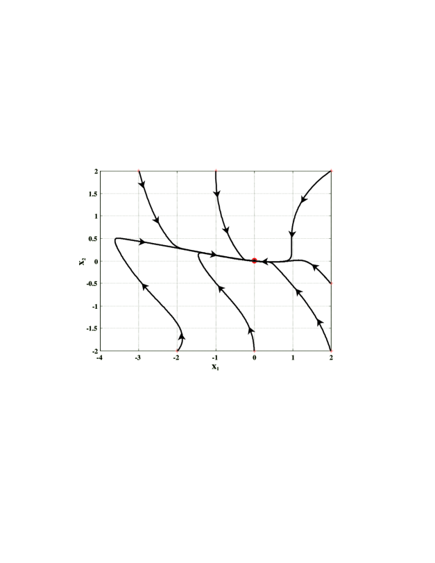
Figure 2: Simulation result for the closed loop system.

6 Conclusions

The controller design for bilinear systems is a very complicated task and only a few results for higher dimensional systems are available. Most of the recent publications treat systems with asymptotically stable system matrix in the linear part. In this paper the existence of a quadratic CLF for bilinear systems has been analysed systematically for the case of two dimensional systems with one input. This case is important because no systematic study for two dimensional systems has been carried out so far and the conditions (2) simplify with increasing number of inputs. Therefore, two dimensional systems with one input represent the first interesting case which has not been treated systematically up to now. We give necessary and sufficient conditions which ensure that the design condition (4) can be satisfied. The result of the complete analysis is presented as a flow diagram which guides the user through the controller design. This is the first complete systematic study of the conditions (2) for a whole class of bilinear systems. In previous research only special examples have been treated or the case of bilinear systems with asymptotically stable system matrix of the linear part has been investigated. The important case with an unstable system matrix of the linear part has not been treated in the literature so far. This gap is closed by the results of this paper for the case of two dimensional bilinear systems with one input. An example illustrating the design is given at the end of the paper.

References

- [1] E.D. Sontag, “A ’universal’ construction of Artstein’s theorem on nonlinear stabilization”, Systems Control Lett., Vol. 13, pp. 117–123, 1989.
- [2] P.-O. Gutman, “Stabilizing controllers for bilinear systems”, IEEE Transactions on Automatic Control, Vol. AC-26, No. 4, pp. 917 – 922, 1981.
- [3] Z. Artstein, “Stabilization with relaxed controls”, Nonlinear Anal., pp. 1163–1173, 1983.
- [4] A. Isidori, Nonlinear Control Systems, Springer, London, Third edition, 1995.
- [5] R. R. Mohler, Nonlinear Systems, Vol. II, Prentice Hall, Englewood Cliffs, New Jersey, 1991.
- [6] D. Redfern, The Maple Handbook, Springer, New York, Heidelberg, First edition, 1993.
- [7] David G. Luenberger, Linear and Nonlinear Programming, Addison-Wesley, Second edition, 1984.
- [8] P. Lancaster and M. Tismenetsky, The Theory of Matrices, Academic Press Inc., Orlando, Second edition, 1985.