The Most Refined Vassiliev Invariant of Degree One
of Knots and Links
in ${\mathbb{R}}^{1}$-fibrations over a surface

Abstract.

As it is well-known, all Vassiliev invariants of degree one of a knot $K\subset{\mathbb{R}}^{3}$ are trivial. There are nontrivial Vassiliev invariants of degree one, when the ambient space is not ${\mathbb{R}}^{3}$. Recently, T. Fiedler introduced such invariants of a knot in an ${\mathbb{R}}^{1}$-fibration over a surface $F$. They take values in the free ${\mathbb{Z}}$-module generated by all the free homotopy classes of loops in $F$. Here, we generalize them to the most refined Vassiliev invariant of degree one. The ranges of values of all these invariants are explicitly described.

We also construct a similar invariant of a two-component link in an ${\mathbb{R}}^{1}$-fibration. It generalizes the linking number.

Most proofs in this paper are postponed till the last section.

Everywhere in this text ${\mathbb{R}}^{1}$-fibration means a locally-trivial fibration with fibers, homeomorphic to ${\mathbb{R}}^{1}$.

We work in the differential category.

1. Invariants of knots and links

1.1. Basic definitions

We say, that a one-dimensional submanifold $L$ of a total space $N^{3}$ of a fibration $p:N^{3}\rightarrow M^{2}$ is generic with respect to $p$ , if $p\big{|}_{L}$ is a generic immersion. An immersion of a one-manifold into a surface is said to be generic, if it has neither self-intersection points of multiplicity greater than two, nor self-tangency points, and at each double point its branches are transversal to each other. An immersion of (a circle) $S^{1}$ to a surface is called a curve.

Let $F$ be a connected smooth two-dimensional surface (not necessarily compact or orientable) and $p:E\rightarrow F$ be an ${\mathbb{R}}^{1}$-fibration with oriented total space $E$. Let $K\subset E$ be a (smooth) oriented knot, in general position with respect to $p$.

Definition 1.1.1 (Fiedler [1]).

Let $q$ be a double point of $p(K)$. Fix an orientation on the fiber $E_{q}=p^{-1}(q)$. This determines, which of the two branches of $K$, intersecting $E_{q}$, is over-crossing and which is under-crossing. Define local writhe $\omega(q)$ to be one if the three-frame (under-crossing, over-crossing, fiber $E_{q}$) agrees with the orientation on $E$ and minus one, otherwise. (It is easy to check, that this definition does not depend on the choice of an orientation on $E_{q}$.)

1.2. Direct generalization of Fiedler’s invariants

In [1] T. Fiedler introduced invariants of a knot $K$ in an oriented total space of an ${\mathbb{R}}^{1}$-fibration $p:E\rightarrow F$. As it follows from [2], these invariants can be expressed through an invariant $U_{K}$, introduced below. If $F$ is oriented, then $U_{K}$ also can be expressed through Fiedler’s invariants. The formulas, expressing them through each other (see [2]), involve the values of all these invariants on some fixed knot homotopic to $K$.

Let $q\in p(K)$ be a crossing point. Split the curve $p(K)$ at $q$ according to the orientation and obtain two oriented loops on $F$ (see Figure 1).

Figure 1.

Definition 1.2.1.

For a crossing point $q$ of $p(K)$ denote by $\xi_{1}(q)$ and $\xi_{2}(q)$ the free homotopy classes of the two loops, created by splitting at $q$. Let $H$ be the free ${\mathbb{Z}}$-module generated by the set of all the free homotopy classes of oriented loops on $F$. Define $U_{K}\in H$ by the following formula, where the summation is taken over all the crossings, such that none of the two loops, created by splitting, is homotopic to a trivial loop.

(1) $$U_{K}=\sum_{\{q\in Q|\xi_{1}(q),\xi_{2}(q)\neq e\}}\omega(q)\Bigl{(}\xi_{1}(q)+\xi_{2}(q)\Bigr{)}$$

Theorem 1.2.2.

$U_{K}$ is an isotopy invariant of the knot $K$.

The proof is straightforward. One checks, that $U_{K}$ does not change under all the oriented versions of the three Reidemeister moves.

1.2.3.

Similarly to [1], one can introduce a version of $U_{K}$, which takes values in ${\mathbb{Z}}[H_{1}(F)]$. To obtain it, one substitutes $\xi_{1}(q)$ and $\xi_{2}(q)$ in (1) by the homology classes, realized by the corresponding loops. The summation should be made over the set of all the double points of $p(K)$, such that none of the two loops created by the splitting is homologous to $0$.

1.2.4.

Let $p:E\rightarrow F$ be an ${\mathbb{R}}^{1}$-fibration over a surface. Let $K\subset E$ be a knot generic with respect to $p$ and $q$ be a crossing point of $p(K)$. The modification of pushing of one branch of $K$ through the other along a fiber $E_{q}$ is called the modification (of the knot) along the fiber $E_{q}$.

Theorem 1.2.5.

(Cf. Fiedler [1]) Let $q$ be a crossing point of $p(K)$. Denote by $i$ and $j$ the free homotopy classes of the two loops, created by splitting of $p(K)$ at $q$ according to the orientation. Under the modification along $E_{q}$ the jump of $U_{K}$ is

(2) $$\begin{cases}\pm 2\Bigl{(}i+j\Bigr{)},&\text{ if }i,j\neq e,\\ 0,&\text{ otherwise. }\end{cases}$$

Here the sign depends on $\omega(q)$.

The proof is straightforward.

Corollary 1.2.6.

$U_{K}$ is a Vassiliev invariant of degree one.

To get the proof, one notices, that the first derivative of $U_{K}$ depends only on the free homotopy classes of the two loops, that appear, if one splits the singular knot (with one transverse double point) at the double point according to the orientation. Hence, the second derivative of $U_{K}$ is identically $0$.

1.3. The most refined Vassiliev invariant of degree one.

1.3.1.

Unfortunately $U_{K}$ appears to be not the most refined Vassiliev invariant of degree one of a knot in an ${\mathbb{R}}^{1}$-fibration. To show this, we construct two knots $K_{1}$ and $K_{2}$ and a first degree Vassiliev invariant $\tilde{U}_{K}$, such that $U_{K_{1}}=U_{K_{2}}$, and $\tilde{U}_{K_{1}}\neq\tilde{U}_{K_{2}}$.

Definition 1.3.2 (of $\tilde{U}_{K}$).

Let $\Gamma$ be an oriented figure eight graph (bouquet of two circles), $V_{\Gamma}$ be its vertex and $E^{1}_{\Gamma}$ and $E^{2}_{\Gamma}$ be its edges. Set $S$ to be a set of free homotopy classes of mappings of $\Gamma$ into $F$, factorized by an orientation preserving involution of $\Gamma$. Let $G$ be the free ${\mathbb{Z}}$-module generated by $S$. For a double point $q$ of $p(K)$ put $G_{q}\in S$ to be the class of the mapping of $\Gamma$, which sends $V_{\Gamma}$ to $q$, $E^{1}_{\Gamma}\cup E^{2}_{\Gamma}$ onto $p(K)$, according to the orientations of the edges, and is injective on the complement of the preimages of the double points of $p(K)$. Let $S^{\prime}\subset S$ be those classes, for which none of the two loops of the figure eight graph is homotopic to a trivial loop. Define $\tilde{U}_{K}\in G$ by the following formula, where the summation is taken over the set of all the crossings $q$ of $p(K)$, such that $G_{q}\in S^{\prime}$.

$$\tilde{U}_{K}=\sum_{\{q\in p(K)|G_{q}\in S^{\prime}\}}\omega(q)G_{q}$$

Figure 2.

Similarly to 1.2.6 one checks, that $\tilde{U}_{K}$ is a Vassiliev invariant of degree one.

Let $F$ be a disc with two holes. Let $K_{1}$ be the knot, shown on Figure 3, and $K_{2}$ be the knot obtained from $K_{1}$ by modifications along fibers over the crossing points $u$ and $v$. (The two shaded discs on Figure 3 are the two holes.) One can easily check, that $U_{K_{1}}=U_{K_{2}}$, but $\tilde{U}_{K_{1}}\neq\tilde{U}_{K_{2}}$.

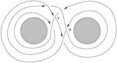
Figure 3.

The following theorem shows, that $\tilde{U}_{K}$ invariant is the most refined Vassiliev invariant of degree one.

Theorem 1.3.3.

Let $v_{1}(K)$ be any Vassiliev invariant of degree one. It induces a mapping $v_{1}^{*}:G\rightarrow{\mathbb{Z}}$, which maps a class of the projection of a singular knot $K^{\prime}$ to $v_{1}(K^{\prime})$. Fix some knot $K_{f}$. Then for any knot $K$, which is free homotopic to $K_{f}$

(3) $$v_{1}(K)=v_{1}(K_{f})+\frac{1}{2}v_{1}^{*}(\tilde{U}_{K}-\tilde{U}_{K_{f}}).$$

1.3.4.

Proof of Theorem 1.3.3.

One can obtain $K$ from $K_{f}$ by a sequence of isotopies and modifications along fibers. Both $v_{1}$ and $\tilde{U}_{K}$ are invariant under isotopy. If under a modification along a fiber $\tilde{U}_{K}$ jumps by $2G_{q}$, then $v_{1}$ jumps by $2v_{1}^{*}(G_{q})$. (Clearly $v_{1}$ does not jump under modification along a fiber, for which one of the two loops of $G_{q}$ is homotopic to a trivial loop.) The total jump of $\tilde{U}_{K}$ under the homotopy is $\tilde{U}_{K_{f}}-\tilde{U}_{K}$. Thus the corresponding jump of $v_{1}$ invariant is $v_{1}(K_{f})-v_{1}(K)=\frac{1}{2}v_{1}^{*}(\tilde{U}_{K_{f}}-\tilde{U}_{K})$ and we proved the theorem. ∎

It is natural to take the simplest knot in the corresponding class as the $K_{f}$ knot. Unfortunately, there is no canonical way to choose one.

As a corollary of Theorem 1.3.3 we get, that for any Vassiliev invariant of degree one — $v_{1}$ and two homotopic knots $K_{1}$ and $K_{2}$, equality $\tilde{U}_{K_{1}}=\tilde{U}_{K_{2}}$ implies $v_{1}(K_{1})=v_{1}(K_{2})$.

The following theorem, characterizes the range of values $\tilde{U}_{K}$.

Theorem 1.3.5.

For a singular knot $K_{s}$ (whose only singularity is a transverse double point) denote by $\bar{K}_{s}$ the free homotopy class of knots, that contains $K_{s}$. For a knot $K$ denote by $G_{K}$ the submodule of $G$ generated by the classes of the projections of singular knots $K_{s}$, such that $K\in\bar{K}_{s}$.

I: Let $K$ and $K^{\prime}$ be two oriented knots, representing the same free homotopy class. Then $\tilde{U}_{K}$ and $\tilde{U}_{K^{\prime}}$ are congruent modulo the $2G_{K}$ submodule.

II: Let $K$ be an oriented knot, $\tilde{U}$ be an element of $G$, such that it is congruent to $\tilde{U}_{K}$ modulo the $2G_{K}$ submodule. Then there exists an oriented knot $K^{\prime}$, such that:

a) $K$ and $K^{\prime}$ represent the same free homotopy class.

b) $\tilde{U}_{K^{\prime}}=\tilde{U}$.

For the proof of Theorem 1.3.5 see Section 2.1.

1.3.6.

There is a natural mapping $\phi:G\rightarrow H$, which maps $g\in G$ to a formal sum of the free homotopy classes of the two loops of $g$. Clearly, $\phi(\tilde{U}_{K})=U_{K}$. (The $\ker(\phi)$ is nontrivial and this is the reason, why $U_{K}$ is not the most refined invariant of degree one.) Using $\phi$ and Theorem 1.3.5 we obtain the following characterization of the range of values of $U_{K}$.

I: If $K$ and $K^{\prime}$ are two oriented knots representing the same free homotopy class, then $U_{K}$ and $U_{K^{\prime}}$ are congruent modulo the $\phi(2G_{K})$ submodule.

II: Let $K$ be an oriented knot, $U$ be an element of $H$, such that it is congruent to $U_{K}$ modulo the $\phi(2G_{K})$ submodule. Then, there exists an oriented knot $K^{\prime}$, such that:

a) $K$ and $K^{\prime}$ represent the same free homotopy class.

b) $U_{K^{\prime}}=U$.

1.4. Partial linking polynomial

Let $\Theta$ be an annulus. Consider a solid torus $T$ embedded into ${\mathbb{R}}^{3}$, and a projection $p:{\mathbb{R}}^{3}\rightarrow{\mathbb{R}}^{2}$, such that $\Im(p\big{|}_{T})$ is homeomorphic to $\Theta$. Let $K\subset T$ be an oriented knot, in general position with respect to $p$. We denote by $i_{1}(q)\text{ and }i_{2}(q)$ the homology classes in $H_{1}(\Theta)$ of the two loops, that are created by splitting of $p(K)$ at the double point $q$. Since $H_{1}(\Theta)={\mathbb{Z}}$ we can consider $i_{1}(q)$ and $i_{2}(q)$ as integer numbers.

Definition 1.4.1 (Aicardi [3]).

Set partial linking polynomial $A(K)$ (originally in [3] it was denoted by $s[K]$) to be a finite Laurent polynomial, defined by the following formula

$$A(K)=\sum_{\{q\in Q|i_{1}(q),i_{2}(q)\neq 0\}}\frac{1}{2}\Bigl{(}\omega(q)(t^{i_{1}(q)}+t^{i_{2}(q)})\Bigr{)}.$$

Below by $a_{i}$ we denote the coefficient of $t^{i}$ in $A(K)$.

1.4.2.

The set of all the free homotopy classes of oriented loops in $\Theta$ coincides with $H_{1}(\Theta)$. One can easily see, that $U_{K}$ is mapped to $2A(K)$ under the natural isomorphism $\psi:H\rightarrow{\mathbb{Z}}[q,q^{-1}]$.

The fact, that $\pi_{1}(T)={\mathbb{Z}}$ allows one to reconstruct an element $g\in G$ from the homology classes of the two loops of it. Thus, in this case $\tilde{U}_{K}$ invariant can also be reconstructed from $A(K)$.

1.4.3Aicardi [3].

Let $h\in{\mathbb{Z}}$ be the image of $[p(K)]$ (the homology class realized by $p(K)$) under the natural identification of $H_{1}(\Theta)$ with ${\mathbb{Z}}$. Then $a_{0}=a_{h}=0$ and $a_{i}=a_{h-i}$ for an arbitrary $i\in{\mathbb{Z}}$.

1.4.4.

One can see, that the very definition of $A(K)$ depends on the embedding of $T$ into ${\mathbb{R}}^{3}$. It is well known, that the group of orientation preserving autohomeomorphisms of $T$, factorized by isotopy relation, is isomorphic to ${\mathbb{Z}}$. It is generated by the class of an autohomeomorphism $\Phi$, that extends a positive Dehn twist along a meridian of $\partial T$. That is cutting $T$ along a meridional disc, twisting by $2\pi$ in a positive direction and gluing back. Replacement of the embedding of $T$ to ${\mathbb{R}}^{3}$ by an isotopic one does not change $A(K)$. Embeddings of all isotopic classes can be obtained from the given one by a composition with $\Phi^{n}$ for some $n\in{\mathbb{Z}}$.

Let $A^{\prime}(K)$ be the partial linking polynomial calculated, after we compose our embedding of $T$ with $\Phi$. Put

$$\Delta A(K)=A^{\prime}(K)-A(K).$$

Let $h\in{\mathbb{Z}}$ be the homology class realized by $p(K)$.

Theorem 1.4.5.

$$\Delta A(K)=\begin{cases}-|h|(t^{1}+t^{2}+\dots+t^{h-1}),&\text{if }h>0\\ -|h|(t^{-1}+t^{-2}+\dots+t^{h+1}),&\text{if }h<0\\ 0,&\text{if }h=0\end{cases}$$

For the proof of Theorem 1.4.5 see Section 2.2.

As we can make the composition of our embedding with $\Phi^{n}$, for any $n\in{\mathbb{Z}}$, we obtain the following.

1.4.6.

$A(K)$ as an invariant of the topological pair $K\subset T$ is defined up to an addition of $\Delta A(K)$. Thus, an $A(K)$ invariant of a knot $K$, could be said to be in a canonical form, if it satisfies the following conditions:

$$\begin{cases}0\leq a_{1}<h&\text{for }h>0,\\ 0\leq a_{-1}<|h|&\text{for }h<0,\\ \end{cases}$$

If $h=0$, then $A(K)$ is always in the canonical form.

Theorem 1.4.7.

Fix $h\in{\mathbb{Z}}$. Let $P_{h}$ be a subset of all finite Laurent polynomials $\sum_{i=i_{1}}^{i_{2}}p_{i}t^{i}$, satisfying the following properties:

a) $p_{0}=p_{h}=0$

b) $\forall j\in{\mathbb{Z}}\quad p_{j}=p_{h-j}$

c) if $h=2k$ for some $k\in{\mathbb{Z}}$ then $p_{k}$ is odd.

Then $P_{h}$ is the range of values of the partial linking polynomial for knots homologous to $h$.

For the proof of Theorem 1.4.7 see Section 2.3.

1.5. Invariant of links

Definition 1.5.1 (of $U_{L}$).

Let $p:E\rightarrow F$ be an ${\mathbb{R}}^{1}$-fibration, of an oriented space $E$ over a surface. Let $\Gamma$ be an oriented figure eight graph (bouquet of two circles), $V_{\Gamma}$ be its vertex and $E^{1}_{\Gamma}$ and $E^{2}_{\Gamma}$ be its edges. Set $\bar{S}$ to be a set of all the free homotopy classes of mappings of $\Gamma$ into $F$. Denote by $\bar{G}$ the free ${\mathbb{Z}}$-module generated by $\bar{S}$. Let $K_{1}\cup K_{2}=L\subset E$ be an oriented two-component link, in general position with respect to $p$. Note, that local writhe $\omega(q)$ is well defined for a point $q\in p(K_{1})\cap p(K_{2})$. Let $\bar{G}_{q}\in\bar{S}$ be the class of the mapping of $\Gamma$ onto $p(K_{1})\cup p(K_{2})$, which maps $V_{\Gamma}$ to $q$, $E^{1}_{\Gamma}$ to $p(K_{1})$, $E^{2}_{\Gamma}$ to $p(K_{2})$ (according to the orientations of the edges) and is injective on the complement of the preimage of the double points of $p(L)$. Define $U_{L}\in\bar{G}$ by the following formula, where the summation is taken over $p(K_{1})\cap p(K_{2})$

(4) $$U_{L}=\sum_{q\in p(K_{i})\cap p(K_{j})}\omega(q)\bar{G}_{q}$$

Theorem 1.5.2.

$U_{L}$ is an isotopy invariant of the link $L$.

The proof of Theorem 1.5.2 is straightforward. One just has to check, that $U_{L}$ is invariant under all the oriented versions of the Reidemeister moves.

1.5.3.

If $E={\mathbb{R}}^{3}$ and $F={\mathbb{R}}^{2}$, then $\bar{G}={\mathbb{Z}}$ (as $\pi_{1}({\mathbb{R}}^{2})=e)$. Under this identification $U_{L}=2\operatorname{lk}(K_{1},K_{2})$, where $\operatorname{lk}(K_{1},K_{2})$ is the linking number of the two knots.

1.5.4.

Let $L=K_{1}\cup\dots\cup K_{n}\subset E$ be a generic $n$-component oriented link. For $i>j$ ($i,j\in\{1,\dots,n\}$) set $L_{ij}$ to be the two component sublink of $L$, consisting of $K_{i}$ and $K_{j}$. Similarly to Theorem 1.3.3, one can see, that the ordered set of the invariants $U_{K_{i}}$ and $U_{L_{ij}}$ ($i>j$) is the most refined degree one Vassiliev invariant of $L$.

2. Proofs

2.1. Proof of Theorem 1.3.5.

I: $K^{\prime}$ can be obtained from $K$ by a sequence of isotopies and modifications along fibers. Isotopies do not change $\tilde{U}$. The modifications change $\tilde{U}$ by elements of $2G_{K}$. Thus, the first part of the theorem is proved.

II: We prove that for any $g\in G_{K}$ there exist two knots $K_{1}$ and $K_{2}$ such, that they represent the same free homotopy class as $K$ and

$$\tilde{U}_{K_{1}}=\tilde{U}_{K}-2g$$

$$\tilde{U}_{K_{2}}=\tilde{U}_{K}+2g$$

Clearly, this implies the second statement of the theorem. To obtain the two knots we isotopically deform $K$ so that $\pi(K)$ bites itself in the projection (as it is shown in Figure 4) and $G_{u}=G_{v}=g$. To obtain $K_{1}$, one performs a fiber modification along $\pi^{-1}(u)$. To obtain $K_{2}$, one performs a fiber modification along $\pi^{-1}(v)$.

Figure 4.

This finishes the proof of Theorem 1.3.5. ∎

2.2. Proof of Theorem 1.4.5.

Let $D$ be a meridional disc along the boundary of which, we performed the positive Dehn twist (used to define $\Phi$). Assume, that all the branches of K, which cross $D$, are perpendicular to it and are located on different levels (see Figure 5). Using second Reidemeister moves transform the diagram in such a way, that if we traverse $K$ along the orientation, then the branches cross $D$ in the order shown in Figure 5. (The thick dashed line in Figure 5 is $p(D)$).

Figure 5.

After we compose the embedding of $T$ with $\Phi$, the diagram will be changed, as it is shown in Figure 6.

Figure 6.

Note, that under the modification of pushing of one branch of the knot through the other, which happens outside of the neighborhood of $D$ (shown in Figure 6) $A(K)$ and $A^{\prime}(K)$ change in the same way. Hence, their difference is preserved. Thus, we can assume that our knot $K$ has an ascending diagram. After a simple calculation we get the desired result. ∎

2.3. Proof of Theorem 1.4.7.

The relation between $U$ and $A$ invariants, shown in 1.4.2, allows one to use 1.3.6 in the case of a partial linking polynomial. There is a natural bijection between one-dimensional homology classes of $T$ and free homotopy classes of oriented loops in $T$.

Thus we get, that:

a) If $K$ and $K^{\prime}$, are such that $[p(K)]=[p(K^{\prime})]=h$, then $A(K^{\prime})$ and $A(K)$ are congruent modulo the additive subgroup generated by all the elements of type

(5) $$\pm(t^{j}+t^{h-j})\text{ for }j\not\in\{h,0\}$$

(Note that if $h=2j$ then this expression is equal to $\pm 2t^{j}$.)

b) Let $K$ be a knot (with $[p(K)]=h$), and let $A$ be a finite Laurent polynomial congruent to $A(K)$ modulo the additive subgroup, generated by all the elements of type (5). Then there exists a knot $K^{\prime}$, such that $[p(K^{\prime})]=h$ and $A(K^{\prime})=A$.

Thus, if $K$ and $K^{\prime}$ are knots such, that $[p(K)]=[p(K^{\prime})]=h$ and $A(K)\in P_{h}$, then $A(K^{\prime})\in P_{h}$. And vice versa, if for some $p_{h}\in P_{h}$ there exists a knot $K_{p_{h}}$, such that $[p(K_{p_{h}})]=h$ and $A(K_{p_{h}})=p_{h}$, then such a knot exists for any $\tilde{p}_{h}\in P_{h}$. Hence, to prove the theorem it is sufficient to show, that for any $h\in{\mathbb{Z}}$ there exists a knot $K_{h}$, such that $[p(K_{h})]=h$ and $A(K_{h})\in P_{h}$. Let $K_{h}$ be a knot, that rotates $h$ times in $T$ and has an ascending diagram (see Figure 7). The $A$ invariant of it is equal to (6) and it belongs to $P_{h}$.

(6) $$\begin{cases}t^{1}+t^{2}+\dots+t^{h-1},&\text{if }h>0\\ t^{-1}+t^{-2}+\dots+t^{h+1},&\text{if }h<0\\ 0,&\text{if }h=0\\ \end{cases}$$

Figure 7.

This finishes the proof of Theorem 1.4.7. ∎

Acknowledgements

I am deeply grateful to Oleg Viro for the inspiration of this work and all the enlightening discussions. I am thankful to Francesca Aicardi, Thomas Fiedler and Michael Polyak for all the valuable discussions we had.

References

- [1] T. Fiedler, A small state sum for knots, Topology 30 (1993) no.2, 281-294
- [2] V. Tchernov First degree Vassiliev invariants of knots in - and -fibrations preprint, Uppsala, Sweden 1996
- [3] F. Aicardi, Invariant Polynomial of Framed Knots in the Solid Torus and its Applications to Wave Fronts and Legendrian Knots, J. of Knot Th. and Ramif, Vol 15, No. 6, (1996), 743-778