Asymptotics of Plancherel measures for symmetric groups

Abstract.

We consider the asymptotics of the Plancherel measures on partitions of $n$ as $n$ goes to infinity. We prove that the local structure of a Plancherel typical partition in the middle of the limit shape converges to a determinantal point process with the discrete sine kernel.

On the edges of the limit shape, we prove that the joint distribution of suitably scaled 1st, 2nd, and so on rows of a Plancherel typical diagram converges to the corresponding distribution for eigenvalues of random Hermitian matrices (given by the Airy kernel). This proves a conjecture due to Baik, Deift, and Johansson by methods different from the Riemann-Hilbert techniques used in their original papers [2, 3] and from the combinatorial proof given in [23].

Our approach is based on an exact determinantal formula for the correlation functions of the poissonized Plancherel measures in terms of a new kernel involving Bessel functions. Our asymptotic analysis relies on the classical asymptotic formulas for the Bessel functions and depoissonization techniques.

1. Introduction

1.1. Plancherel measures

Given a finite group $G$, by the corresponding Plancherel measure we mean the probability measure on the set $G^{\wedge}$ of irreducible representations of $G$ which assigns to a representation $\pi\in G^{\wedge}$ the weight $(\dim\pi)^{2}/|G|$. For the symmetric group $S(n)$, the set $S(n)^{\wedge}$ is the set of partitions $\lambda$ of the number $n$, which we shall identify with Young diagrams with $n$ squares throughout this paper. The Plancherel measure on partitions $\lambda$ arises naturally in representation–theoretic, combinatorial, and probabilistic problems. For example, the Plancherel distribution of the first part of a partition coincides with the distribution of the longest increasing subsequence of a uniformly distributed random permutation [28].

We denote the Plancherel measure on partitions of $n$ by $M_{n}$

(1.1) $$M_{n}(\lambda)=\frac{(\dim\lambda)^{2}}{n!}\,,\quad|\lambda|=n\,,$$

where $\dim\lambda$ is the dimension of the corresponding representation of $S(n)$. The asymptotic properties of these measures as $n\to\infty$ have been studied very intensively, see the References and below.

In the seventies, Logan and Shepp [21] and, independently, Vershik and Kerov [36, 38] discovered the following measure concentration phenomenon for $M_{n}$ as $n\to\infty$. Let $\lambda$ be a partition of $n$ and let $i$ and $j$ be the usual coordinates on the diagrams, namely, the row number and the column number. Introduce new coordinates $u$ and $v$ by

$$u=\frac{j-i}{\sqrt{n}}\,,\quad v=\frac{i+j}{\sqrt{n}}\,,$$

that is, we flip the diagram, rotate it $135^{\circ}$ as in Figure 1, and scale it by the factor of $n^{-1/2}$ in both directions.

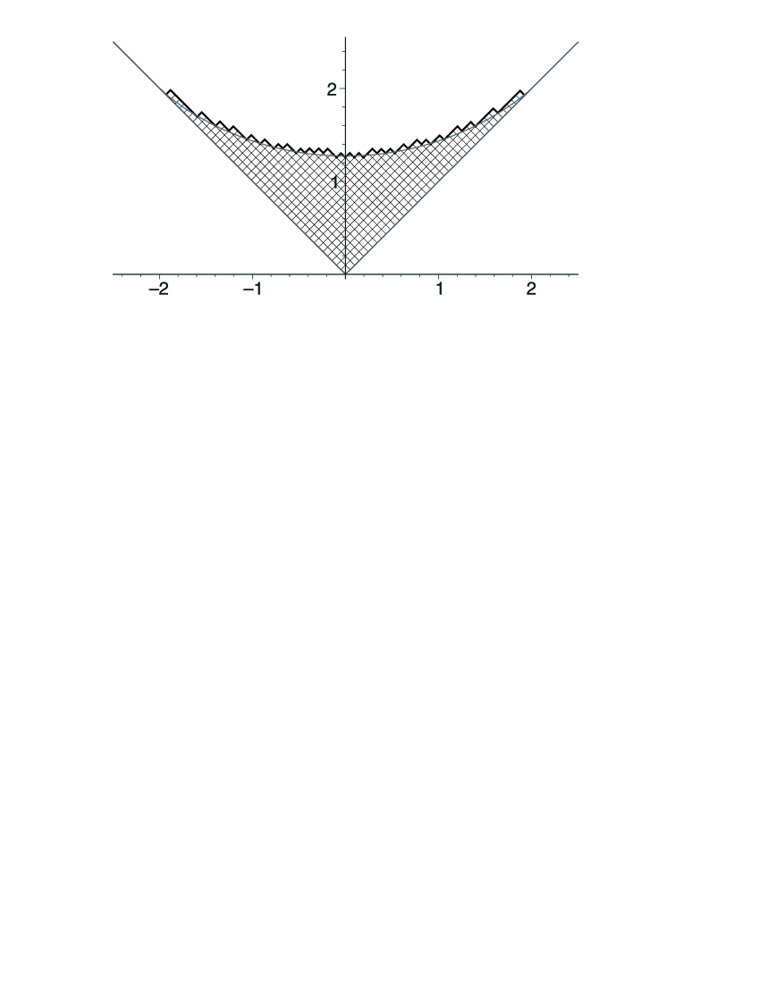
Figure 1. The limit shape of a typical diagram.

After this scaling, the Plancherel measures $M_{n}$ converge as $n\to\infty$ (see [21, 36, 38] for precise statements) to the delta measure supported on the following shape:

$$\{|u|\leq 2,|u|\leq v\leq\Omega(u)\}\,,$$

where the function $\Omega(u)$ is defined by

$$\Omega(u)=\begin{cases}{\frac{2}{\pi}\,\left(u\arcsin(u/2)+\sqrt{4-u^{2}}\right)}\,,&|u|\leq 2\,,\\ |u|\,,&|u|>2\,.\end{cases}$$

The function $\Omega$ is plotted in Figure 1. As explained in great detail in [20], this limit shape $\Omega$ is very closely connected to Wigner’s semicircle law for distribution of eigenvalues of a random matrices, see also [17, 18, 19].

From a different point of view, the connection with random matrices was observed in [2, 3], and also in the earlier papers [14, 25, 26]. In [2], Baik, Deift, and Johansson made the following conjecture. They conjectured that in the $n\to\infty$ limit and after proper scaling the joint distribution of $\lambda_{i}$, $i=1,2,\dots$ becomes identical to the joint distribution of largest eigenvalues of a Gaussian random Hermitian matrix (which is known to be the so-called Airy ensemble, see Section 1.4). They proved this for the individual distribution of $\lambda_{1}$ and $\lambda_{2}$ in [2] and [3], respectively. A combinatorial proof of the full conjecture was given by one of us in [23]. It was based on an interplay between maps on surfaces and ramified coverings of the sphere.

In this paper we study the local structure of a typical Plancherel diagram both in the bulk of the limit shape $\Omega$ and on its edge, where by the study of the edge we mean the study of the behavior of $\lambda_{1}$, $\lambda_{2}$, and so on.

We employ an analytic approach based on an exact formula in terms of Bessel functions for the correlation functions of the so-called poissonization of the Plancherel measures $M_{n}$, see Theorem 1 in the following section, and the so-called depoissonization techniques, see Section 1.4.

The exact formula in Theorem 1 is a limit case of a formula from [6], see also the recent paper [24] for a more general result. The use of poissonization and depoissonization is very much in the spirit of [2, 14, 35] and represents a well known in statistical mechanics principle of the equivalence of ensembles.

Our main results are the following two. In the bulk of the limit shape $\Omega$, we prove that the local structure of a Plancherel typical partition converges to a determinantal point process with the discrete sine kernel, see Theorem 3. This result is parallel to the corresponding result for random matrices. On the edge of the limit shape, we give an analytic proof of the Baik-Deift-Johansson conjecture, see Theorem 4. These results will be stated in Subsections 1.3 and 1.4 of the present Introduction, respectively.

Simultaneously and independently, results equivalent to our Theorems 2 and 4 were obtained by K. Johansson [15].

1.2. Poissonization and correlation functions

For $\theta>0$, consider the poissonization $M^{\theta}$ of the measures $M_{n}$

$$M^{\theta}(\lambda)=e^{-\theta}\sum_{n}\frac{\theta^{n}}{n!}\,M_{n}(\lambda)=e^{-\theta}\theta^{|\lambda|}\,\left(\frac{\dim\lambda}{|\lambda|!}\right)^{2}\,.$$

This is a probability measure on the set of all partitions. Our first result is the computation of the correlation functions of the measures $M^{\theta}$.

By correlation functions we mean the following. By definition, set

$$\mathcal{D}(\lambda)=\{\lambda_{i}-i\}\subset\mathbb{Z}\,.$$

Also, following [37], define the modified Frobenius coordinates $\operatorname{Fr}(\lambda)$ of a partition $\lambda$ by

(1.2) $$\operatorname{Fr}(\lambda)=\left(\mathcal{D}(\lambda)+{\textstyle\frac{1}{2}}\right)\triangle\left(\mathbb{Z}_{\leq 0}-{\textstyle\frac{1}{2}}\right)\\ =\left\{p_{1}+{\textstyle\frac{1}{2}},\dots,p_{d}+{\textstyle\frac{1}{2}},-q_{1}-{\textstyle\frac{1}{2}},\dots,-q_{d}-{\textstyle\frac{1}{2}}\right\}\subset\mathbb{Z}+{\textstyle\frac{1}{2}}\,,$$

where $\triangle$ stands for the symmetric difference of two sets, $d$ is the number of squares on the diagonal of $\lambda$, and $p_{i}$’s and $q_{i}$’s are the usual Frobenius coordinates of $\lambda$. Recall that $p_{i}$ is the number of squares in the $i$th row to the right of the diagonal, and $q_{i}$ is number of squares in the $i$th column below the diagonal. The equality (1.2) is a well known combinatorial fact discovered by Frobenius, see Ex. I.1.15(a) in [22]. Note that, in contrast to $\operatorname{Fr}(\lambda)$, the set $\mathcal{D}(\lambda)$ is infinite and, moreover, it contains all but finitely many negative integers.

The sets $\mathcal{D}(\lambda)$ and $\operatorname{Fr}(\lambda)$ have the following nice geometric interpretation. Let the diagram $\lambda$ be flipped and rotated $135^{\circ}$ as in Figure 1, but not scaled. Denote by $\omega_{\lambda}$ a piecewise linear function with $\omega^{\prime}_{\lambda}=\pm 1$ whose graph if given by the upper boundary of $\lambda$ completed by the lines

$$v=|u|\,,\quad u\notin[-\lambda^{\prime}_{1},\lambda_{1}]\,.$$

Then

$$k\in\mathcal{D}(\lambda)\Leftrightarrow\omega^{\prime}_{\lambda}\Big{|}_{[k,k+1]}=-1\,.$$

In other words, if we consider $\omega_{\lambda}$ as a history of a walk on $\mathbb{Z}$ then $\mathcal{D}(\lambda)$ are those moments when a step is made in the negative direction. It is therefore natural to call $\mathcal{D}(\lambda)$ the descent set of $\lambda$. As we shall see, the correspondence $\lambda\mapsto\mathcal{D}(\lambda)$ is a very convenient way to encode the local structure of the boundary of $\lambda$.

The halves in the definition of $\operatorname{Fr}(\lambda)$ have the following interpretation: one splits the diagonal squares in half and gives half to the rows and half to the columns.

Definition 1.1.

The correlation functions of $M^{\theta}$ are the probabilities that the sets $\operatorname{Fr}(\lambda)$ or, similarly, $\mathcal{D}(\lambda)$ contain a fixed subset $X$. More precisely, we set

(1.3) $$\rho^{\theta}(X) =M^{\theta}\left(\left\{\lambda\,|\,X\subset\operatorname{Fr}(\lambda)\right\}\right)\,,\quad X\in\mathbb{Z}+{\textstyle\frac{1}{2}}\,,$$

(1.4) $$\boldsymbol{\varrho}^{\theta}(X) =M^{\theta}\left(\left\{\lambda\,|\,X\subset\mathcal{D}(\lambda)\right\}\right)\,,\quad X\in\mathbb{Z}\,.$$

Theorem 1.

For any $X=\{x_{1},\dots,x_{s}\}\subset\mathbb{Z}+{\textstyle\frac{1}{2}}$ we have

$$\rho^{\theta}(X)=\det\Big{[}\mathsf{K}(x_{i},x_{j})\Big{]}_{1\leq i,j\leq s}\,,$$

where the kernel $\mathsf{K}$ is given by the following formula

(1.5) $$\mathsf{K}(x,y)=\left\{\begin{array}[]{ll}\displaystyle\sqrt{\theta}\,\,\frac{\mathsf{k}_{+}(|x|,|y|)}{|x|-|y|}\,,&xy>0\,,\\[10.0pt] \displaystyle\sqrt{\theta}\,\,\frac{\mathsf{k}_{-}(|x|,|y|)}{x-y}\,,&xy<0\,.\end{array}\right.$$

The functions $\mathsf{k}_{\pm}$ are defined by

(1.6) $$\mathsf{k}_{+}(x,y) =J_{x-\frac{1}{2}}\,J_{y+\frac{1}{2}}-J_{x+\frac{1}{2}}\,J_{y-\frac{1}{2}}\,,$$

(1.7) $$\mathsf{k}_{-}(x,y) =J_{x-\frac{1}{2}}\,J_{y-\frac{1}{2}}+J_{x+\frac{1}{2}}\,J_{y+\frac{1}{2}}\,,$$

where $J_{x}=J_{x}(2\sqrt{\theta})$ is the Bessel function of order $x$ and argument $2\sqrt{\theta}$.

This theorem is established in Section 2.1, see also Remark 1.2 below. By the complementation principle, see Sections A.3 and 2.2, Theorem 1 is equivalent to the following

Theorem 2.

For any $X=\{x_{1},\dots,x_{s}\}\subset\mathbb{Z}$ we have

(1.8) $$\boldsymbol{\varrho}^{\theta}(X)=\det\Big{[}\mathsf{J}(x_{i},x_{j})\Big{]}_{1\leq i,j\leq s}\,,$$

Here the kernel $\mathsf{J}$ is given by the following formula

(1.9) $$\mathsf{J}(x,y)=\mathsf{J}(x,y;\theta)=\sqrt{\theta}\,\,\frac{J_{x}\,J_{y+1}-J_{x+1}\,J_{y}}{x-y}\,,$$

where $J_{x}=J_{x}(2\sqrt{\theta})$.

Remark 1.2.

Theorem 1 is a limit case of Theorem 3.3 of [6]. For the reader’s convenience a direct proof of it is given in Section 2. Another proof of the results of [6] will appear in [7]. Various limit cases of the results of [6] are discussed in [8]. By different methods, the formula (1.8) was obtained by K. Johansson [15].

A representation–theoretic proof of a more general formula than Theorem 3.3 of [6] has been subsequently given in [24].

Remark 1.3.

Observe that all Bessel functions involved in the above formulas are of integer order. Also note that the ratios like $\mathsf{J}(x,y)$ are entire functions of $x$ and $y$ because $J_{x}$ is an entire function of $x$. In particular, the values $\mathsf{J}(x,x)$ are well defined. Various denominator–free formulas for the kernel $\mathsf{J}$ are given in Section 2.1.

1.3. Asymptotics in the bulk of the spectrum

Given a sequence of subsets

$$X(n)=\left\{x_{1}(n)<\dots<x_{s}(n)\right\}\subset\mathbb{Z}\,,$$

where $s=|X(n)|$ is some fixed integer, we call this sequence regular if the following limits

(1.10) $$a_{i} =\lim_{n\to\infty}\frac{x_{i}(n)}{\sqrt{n}}\,,$$

(1.11) $$d_{ij} =\lim_{n\to\infty}\left(x_{i}(n)-x_{j}(n)\right)\,,$$

exist, finite or infinite. Here $i,j=1,\dots,s$. Observe that if $d_{ij}$ is finite then $d_{ij}=x_{i}(n)-x_{j}(n)$ for $n\gg 0$.

In the case when $X(n)$ can be represented as $X(n)=X^{\prime}(n)\cup X^{\prime\prime}(n)$ and the distance between $X^{\prime}(n)$ and $X^{\prime\prime}(n)$ goes to $\infty$ as $n\to\infty$ we shall say that the sequence splits; otherwise, we call it nonsplit. Obviously, $X(n)$ is nonsplit if and only if all $x_{i}(n)$ stay at a finite distance from each other.

Define the correlation functions $\boldsymbol{\varrho}(n,\,\cdot\,)$ of the measures $M_{n}$ by the same rule as in (1.4)

$$\boldsymbol{\varrho}(n,X)=M_{n}\left(\left\{\lambda\,|\,X\subset\mathcal{D}(\lambda)\right\}\right)\,.$$

We are interested in the limit of $\boldsymbol{\varrho}(n,X(n))$ as $n\to\infty$. This limit will be computed in Theorem 3 below. As we shall see, if $X(n)$ splits, then the limit correlations factor accordingly.

Introduce the following discrete sine kernel which is a translation invariant kernel on the lattice $\mathbb{Z}$

$$\mathsf{S}(k,l;a)=\mathsf{S}(k-l,a)\,,\quad k,l\in\mathbb{Z}\,,$$

depending on a real parameter $a$:

$$\mathsf{S}(k,a) =\frac{\sin(\arccos(a/2)\,k)}{\pi k}$$

$$=\frac{\sqrt{4-a^{2}}}{2\pi}\frac{U_{k-1}(a/2)}{k}\,,\quad k\in\mathbb{Z}\,.$$

Here $U_{k}$ is the Tchebyshev polynomials of the second kind. We agree that

$$\mathsf{S}(0,a)=\frac{\arccos(a/2)}{\pi}\,,\quad\mathsf{S}(\infty,a)=0$$

and also that

$$\mathsf{S}(k,a)=\begin{cases}0\,,&\textup{$a\geq 2$ or $a\leq 2$ and $k\neq 0$}\,,\\ 1\,,&\textup{$a\leq 2$ and $k=0$}\,.\end{cases}$$

The following result describes the local structure of a Plancherel typical partition.

Theorem 3.

Let $X(n)\subset\mathbb{Z}$ be a regular sequence and let the numbers $a_{i}$, $d_{ij}$ be defined by (1.10), (1.11). If $X(n)$ splits, that is, if $X(n)=X^{\prime}(n)\cup X^{\prime\prime}(n)$ and the distance between $X^{\prime}(n)$ and $X^{\prime\prime}(n)$ goes to $\infty$ as $n\to\infty$ then

(1.12) $$\lim_{n\to\infty}\boldsymbol{\varrho}(n,X(n))=\lim_{n\to\infty}\boldsymbol{\varrho}(n,X^{\prime}(n))\cdot\lim_{n\to\infty}\boldsymbol{\varrho}(n,X^{\prime\prime}(n))\,.$$

If $X(n)$ is nonsplit then

(1.13) $$\lim_{n\to\infty}\boldsymbol{\varrho}\left(n,X(n)\right)=\det\Big{[}\,\mathsf{S}(d_{ij},a)\Big{]}_{1\leq i,j\leq s}\,,$$

where $\mathsf{S}$ is the discrete sine kernel and $a=a_{1}=a_{2}=\dots$.

We prove this theorem in Section 3.

Remark 1.4.

Notice that, in particular, Theorem 3 implies that, as $n\to\infty$, the shape of a typical partition $\lambda$ near any point of the limit curve $\Omega$ is described by a stationary random process. For distinct points on the curve $\Omega$ these random processes are independent.

Remark 1.5.

By complementation, see Section A.3 and 3.2, one obtains from Theorem 3 an equivalent statement about the asymptotics of the following correlation functions

$$\rho(n,X)=M_{n}\left(\left\{\lambda\,|\,X\subset\operatorname{Fr}(\lambda)\right\}\right)\,.$$

Remark 1.6.

The discrete sine kernel was studied before, see [40, 41], mainly as a model case for the continuous sine kernel. In particular, the asymptotics of Toeplitz determinants built from the discrete sign kernel was obtained by H. Widom in [41] answering a question of F. Dyson. As pointed out by S. Kerov, this asymptotics has interesting consequences for the Plancherel measures.

Remark 1.7.

Note that, in particular, Theorem 3 implies that the limit density (the 1-point correlation function) is given by

(1.14) $$\boldsymbol{\varrho}(\infty,a)=\begin{cases}\frac{1}{\pi}\,{\arccos(a/2)}\,,&|a|\leq 2\,,\\ 0\,,&a>2\,,\\ 1\,,&a<-2\,.\end{cases}$$

This is in agreement with the Logan-Shepp-Vershik-Kerov result about the limit shape $\Omega$. More concretely, the function $\Omega$ is related to the density (1.14) by

$$\boldsymbol{\varrho}(\infty,u)=\frac{1-\Omega^{\prime}(u)}{2}\,,$$

which can be interpreted as follows. Approximately, we have

$$\#\left\{i\,\left|\,\frac{\lambda_{i}}{\sqrt{n}}\in[u,u+\Delta u]\right.\right\}\approx\sqrt{n}\,\boldsymbol{\varrho}(\infty,u)\,\Delta u\,.$$

Set $w=\dfrac{i}{\sqrt{n}}$. Then the above relation reads $\Delta w\approx\boldsymbol{\varrho}(\infty,u)\,\Delta u$ and it should be satisfied on the boundary $v=\Omega(u)$ of the limit shape. Since $v=u+2w$, we conclude that

$$\boldsymbol{\varrho}(\infty,u)\approx\frac{dw}{du}=\frac{1-\Omega^{\prime}}{2}\,,$$

as was to be shown.

Remark 1.8.

The discrete sine-kernel $\mathsf{S}$ becomes especially nice near the diagonal, that is, where $a=0$. Indeed,

$$\mathsf{S}(x,0)=\begin{cases}1/2\,,&x=0\,,\\ {(-1)^{(x-1)/2}}\Big{/}(\pi x)\,,&x=\pm 1,\pm 3,\dots\,,\\ 0\,,&x=\pm 2,\pm 4,\dots\,.\end{cases}$$

1.4. Behavior near the edge of the spectrum and the Airy ensemble

The discrete sine kernel $\mathsf{S}(k,a)$ vanishes if $a\geq 2$. Therefore, it follows from Theorem 3 that the limit correlations $\lim\boldsymbol{\varrho}(n,X(n))$ vanish if $a_{i}\geq 2$ for some $i$. However, as will be shown below in Proposition 4.1, after a suitable scaling near the edge $u=2$, the correlation functions $\boldsymbol{\varrho}^{\theta}$ converge to the correlation functions given by the Airy kernel [11, 32]

$$\mathsf{A}(x,y)=\frac{A(x)A^{\prime}(y)-A^{\prime}(x)A(y)}{x-y}\,.$$

Here $A(x)$ is the Airy function:

(1.15) $$A(x)=\frac{1}{\pi}\,\int_{0}^{\infty}\cos\left(\frac{u^{3}}{3}+xu\right)\,du.$$

In fact, the following more precise statement is true about the behavior of the Plancherel measure near the edge $u=2$. By symmetry, everything we say about the edge $u=2$ applies to the opposite edge $u=-2$.

Consider the random point process on $\mathbb{R}$ whose correlation functions are given by the determinants

$$\rho^{\textup{Airy}}_{k}(x_{1},\dots,x_{k})=\det\Big{[}\,\mathsf{A}(x_{i},x_{j})\Big{]}_{1\leq i,j\leq k}$$

and let

$$\zeta=(\zeta_{1}>\zeta_{2}>\zeta_{3}>\dots)\in\mathbb{R}^{\infty}$$

be its random configuration. We call the random variables $\zeta_{i}$’s the Airy ensemble. It is known [11, 32] that the Airy ensemble describes the behavior of the (properly scaled) 1st, 2nd, and so on largest eigenvalues of a Gaussian random Hermitian matrix. The distribution of individual eigenvalues was obtained by Tracy and Widom in [32] in terms of certain Painlevé transcendents.

It has been conjectured by Baik, Deift, and Johansson that the random variables

$$\widetilde{\lambda}=\left(\widetilde{\lambda}_{1}\geq\widetilde{\lambda}_{2}\geq\dots\right)\,,\quad\widetilde{\lambda}_{i}=n^{1/3}\,\left(\frac{\lambda_{i}}{n^{1/2}}-2\right)$$

converge, in distribution and together with all moments, to the Airy ensemble. They verified this conjecture for individual distribution of $\lambda_{1}$ and $\lambda_{2}$ in [2] and [3], respectively. In particular, in the case of $\lambda_{1}$, this generalizes the result of [36, 38] that $\frac{\lambda_{1}}{\sqrt{n}}\to 2$ in probability as $n\to\infty$. The computation of $\lim\frac{\lambda_{1}}{\sqrt{n}}$ was known as the Ulam problem; different solutions to this problem were given in [1, 14, 29].

Convergence of all expectations of the form

(1.16) $$\left\langle\prod_{k=1}^{r}\sum_{i=1}^{\infty}e^{t_{k}\widetilde{\lambda}_{i}}\right\rangle\,,\quad t_{1},\dots,t_{r}>0\,,\quad r=1,2,\dots\,,$$

to the corresponding quantities for the Airy ensembles was established in [23]. The proof in [23] was based on a combinatorial interpretation of (1.16) as the asymptotics in a certain enumeration problem for random surfaces.

In the present paper we use different ideas to prove the following

Theorem 4.

As $n\to\infty$, the random variables $\widetilde{\lambda}$ converge, in joint distribution, to the Airy ensemble.

This is done in Section 4 using methods described in the next subsection. The result stated in Theorem 4 was independently obtained by K. Johansson in [15].

1.5. Poissonization and depoissonization

We obtain Theorems 3 and 4 from Theorem 1 using the so-called depoissonization techniques. We recall that the fundamental idea of depoissonization is the following.

Given a sequence $b_{1},b_{2},b_{3},\dots$ its poissonization is, by definition, the function

(1.17) $$B(\theta)=e^{-\theta}\sum_{k=1}^{\infty}\frac{\theta^{k}}{k!}\,b_{k}\,.$$

Provided the $b_{k}$’s grow not too rapidly this is an entire function of $\theta$. In combinatorics, it is usually called the exponential generating function of the sequence $\{b_{k}\}$. Various methods of extracting asymptotics of sequences from their generating functions are classically known and widely used, see for example [35] where such methods are used to obtain the limit shape of a typical partition under various measures on the set of partitions.

A probabilistic way to look at the generating function (1.17) is the following. If $\theta\geq 0$ then $B(\theta)$ is the expectation of $b_{\eta}$ where $\eta\in\{0,1,2,\dots\}$ is a Poisson random variable with parameter $\theta$. Because $\eta$ has mean $\theta$ and standard deviation $\sqrt{\theta}$, one expects that

(1.18) $$B(n)\approx b_{n}\,,\quad n\to\infty\,,$$

provided the variations of $b_{k}$ for $|k-n|\leq\operatorname{const}\sqrt{n}$ are small. One possible regularity condition on $b_{n}$ which implies (1.18) is monotonicity. In a very general and very convenient form, a depoissonization lemma for nonincreasing nonnegative $b_{n}$ was established by K. Johansson in [14]. We use this lemma in Section 4 to prove Theorem 4.

Another approach to depoissonization is to use a contour integral

(1.19) $$b_{n}=\frac{n!}{2\pi i}\int_{C}\frac{B(z)\,e^{z}}{z^{n}}\,\frac{dz}{z}\,,$$

where $C$ is any contour around $z=0$. Suppose, for a moment, that $b_{n}$ is constant $b=b_{n}=B(z)$. The function $e^{z}/z^{n}=e^{z-n\ln z}$ has a unique critical point $z=n$. If we choose $|z|=n$ as the contour $C$, then only neighborhoods of size $|z-n|\leq\operatorname{const}\sqrt{n}$ contribute to the asymptotics of (1.19). Therefore, for general $\{b_{n}\}$, we still expect that provided the overall growth of $B(z)$ is under control and the variations of $B(z)$ for $|z-n|\leq\operatorname{const}\sqrt{n}$ are small, the asymptotically significant contribution to (1.19) will come from $z=n$. That is, we still expect (1.18) to be valid. See, for example, [13] for a comprehensive discussion and survey of this approach.

We use this approach to prove Theorem 3 in Section 3. The growth conditions on $B(z)$ which are suitable in our situation are spelled out in Lemma 3.1.

In our case, the functions $B(\theta)$ are combinations of the Bessel functions. Their asymptotic behavior as $\theta\approx n\to\infty$ can be obtained directly from the classical results on asymptotics of Bessel functions which are discussed, for example, in the fundamental Watson’s treatise [39]. These asymptotic formulas for Bessel functions are derived using the integral representations of Bessel functions and the steepest descent method. The different behavior of the asymptotics in the bulk $(-2,2)$ of the spectrum, near the edges $\pm 2$ of the spectrum, and outside of $[-2,2]$ is produced by the different location of the saddle point in these three cases.

1.6. Organization of the paper

Section 2 contains the proof of Theorems 1 and 2 and also various formulas for the kernels $\mathsf{K}$ and $\mathsf{J}$. We also discuss a difference operator which commutes with $\mathsf{J}$ and its possible applications.

Section 3 deals with the behavior of the Plancherel measure in the bulk of the spectrum; there we prove Theorem 3. Theorem 4 and a similar result (Theorem 5) for the poissonized measure $M^{\theta}$ are established in Section 4.

At the end of the paper there is an Appendix, where we collected some necessary results about Fredholm determinants, point processes, and convergence of trace class operators.

1.7. Acknowledgements

In many different ways, our work was inspired by the work of J. Baik, P. Deift, and K. Johansson, on the one hand, and by the work of A. Vershik and S. Kerov, on the other. It is our great pleasure to thank them for this inspiration and for many fruitful discussions.

2. Correlation functions of the measures $M^{\theta}$

2.1. Proof of Theorem 1

As noted above, Theorem 1 is a limit case of Theorem 3.3 of [6]. That theorem concerns a family $\{M^{(n)}_{zz^{\prime}}\}$ of probability measures on partitions of $n$, where $z,z^{\prime}$ are certain parameters. When the parameters go to infinity, $M^{(n)}_{zz^{\prime}}$ tends to the Plancherel measure $M_{n}$. Theorem 3.3 in [6] gives a determinantal formula for the correlation functions of the measure

(2.1) $$M^{\xi}_{zz^{\prime}}=(1-\xi)^{t}\,\sum_{n=1}^{\infty}\frac{(t)_{n}}{n!}\,\xi^{n}\,M^{(n)}_{zz^{\prime}}$$

in terms of a certain hypergeometric kernel. Here $t=zz^{\prime}>0$ and $\xi\in(0,1)$ is an additional parameter. As $z,z^{\prime}\to\infty$ and $\xi=\frac{\theta}{t}\to 0$, the negative binomial distribution in (2.1) tends to the Poisson distribution with parameter $\theta$. In the same limit, the hypergeometric kernel becomes the kernel $\mathsf{K}$ of Theorem 1. The Bessel functions appear as a suitable degeneration of hypergeometric functions.

Recently, these results of [6] were considerably generalized in [24], where it was shown how this type of correlation functions computations can be done using simple commutations relations in the infinite wedge space.

For the reader’s convenience, we present here a direct and elementary proof which uses the same ideas as in [6] plus an additional technical trick, namely, differentiation with respect to $\theta$ which kills denominators. This trick yields an denominator–free integral formula for the kernel $\mathsf{K}$, see Proposition 2.7. Our proof here is a verification, not deduction. For more conceptual approaches the reader is referred to [7, 24].

Let $x,y\in\mathbb{Z}+{\textstyle\frac{1}{2}}$. Introduce the following kernel $\mathsf{L}$

$$\mathsf{L}(x,y;\theta)=\begin{cases}0\,,&xy>0\,,\\ \dfrac{1}{x-y}\dfrac{\theta^{(|x|+|y|)/2}}{\Gamma(|x|+{\textstyle\frac{1}{2}})\,\Gamma(|y|+{\textstyle\frac{1}{2}})}\,,&xy<0\,.\end{cases}$$

We shall consider the kernels $\mathsf{K}$ and $\mathsf{L}$ as operators in the $\ell^{2}$ space on $\mathbb{Z}+{\textstyle\frac{1}{2}}$.

We recall that simple multiplicative formulas (for example, the hook formula) are known for the number $\dim\lambda$ in (1.1). For our purposes, it is convenient to rewrite the hook formula in the following determinantal form. Let $\lambda=(p_{1},\dots,p_{d}\,|\,q_{1},\dots,q_{d})$ be the Frobenius coordinates of $\lambda$, see Section 1.2. We have

(2.2) $$\frac{\dim\lambda}{|\lambda|!}=\det\left[\frac{1}{(p_{i}+q_{j}+1)\,p_{i}!\,q_{i}!}\right]_{1\leq i,j\leq d}\,.$$

The following proposition is a straightforward computation using (2.2).

Proposition 2.1.

Let $\lambda$ be a partition. Then

(2.3) $$M^{\theta}(\lambda)=e^{-\theta}\,\det\Big{[}\mathsf{L}(x_{i},x_{j};\theta)\Big{]}_{1\leq i,j\leq s}\,,$$

where $\operatorname{Fr}(\lambda)=\{x_{1},\dots,x_{s}\}\subset\mathbb{Z}+{\textstyle\frac{1}{2}}$ are the modified Frobenius coordinates of $\lambda$.

Let $\operatorname{Fr}_{*}\left(M^{\theta}\right)$ be the push-forward of $M^{\theta}$ under the map $\operatorname{Fr}$. Note that the image of $\operatorname{Fr}$ consists of sets $X\subset\mathbb{Z}+{\textstyle\frac{1}{2}}$ having equally many positive and negative elements. For other $X\subset\mathbb{Z}+{\textstyle\frac{1}{2}}$, the right-hand side of (2.3) can be easily seen to vanish. Therefore $\operatorname{Fr}_{*}\left(M^{\theta}\right)$ is a determinantal point process (see the Appendix) corresponding to $\mathsf{L}$, that is, its configuration probabilities are determinants of the form (2.3).

Corollary 2.2.

$\det(1+\mathsf{L})=e^{\theta}$.

This follows from the fact that $M^{\theta}$ is a probability measure. This is explained in Propositions A.1 and A.4 in the Appendix. Note that, in general, one needs to check that $\mathsf{L}$ is a trace class operator. However, because of the special form of $\mathsf{L}$, it suffices to check a weaker claim – that $\mathsf{L}$ is a Hilbert–Schmidt operator, which is immediate.

Theorem 1 now follows from general properties of determinantal point processes (see Proposition A.6 in the Appendix) and the following

Proposition 2.3.

$\mathsf{K}=\mathsf{L}\,(1+\mathsf{L})^{-1}$.

We shall need three following identities for Bessel functions which are degeneration of the identities (3.13–15) in [6] for the hypergeometric function. The first identity is due to Lommel (see [39], Section 3.2 or [12], 7.2.(60))

(2.4) $$J_{\nu}(2z)\,J_{1-\nu}(2z)+J_{-\nu}(2z)\,J_{\nu-1}(2z)=\frac{\sin\pi\nu}{\pi\,z}\,.$$

The other two identities are the following.

Lemma 2.4.

For any $\nu\neq 0,-1,-2,\dots$ and any $z\neq 0$ we have

(2.5) $$\sum_{m=0}^{\infty}\frac{1}{m+\nu}\frac{z^{m}}{m!}\,J_{m}(2z)=\frac{\Gamma(\nu)\,J_{\nu}(2z)}{z^{\nu}}\,,$$

(2.6) $$\sum_{m=0}^{\infty}\frac{1}{m+\nu}\frac{z^{m}}{m!}\,J_{m+1}(2z)=\frac{1}{z}-\frac{\Gamma(\nu)\,J_{\nu-1}(2z)}{z^{\nu}}\,.$$

Proof.

Another identity due to Lommel (see [39], Section 5.23, or [12], 7.15.(10)) reads

$$\sum_{m=0}^{\infty}\frac{\Gamma(\nu-s+m)}{\Gamma(\nu+m+1)}\frac{z^{m}}{m!}\,J_{m+s}(2z)=\frac{\Gamma(\nu-s)}{\Gamma(s+1)}\,\frac{J_{\nu}(2z)}{z^{\nu-s}}\,.$$

Substituting $s=0$ we get (2.5). Substituting $s=1$ yields

(2.7) $$\sum_{m=0}^{\infty}\frac{1}{(m+\nu)(m+\nu-1)}\frac{z^{m}}{m!}\,J_{m+1}(2z)=\frac{\Gamma(\nu-1)\,J_{\nu}(2z)}{z^{\nu-1}}\,.$$

Let $r(\nu,z)$ the difference of the left-hand side and the right-hand side in (2.6). Using (2.7) and the recurrence relation

(2.8) $$J_{\nu+1}(2z)-\frac{\nu}{z}J_{\nu}(2z)+J_{\nu-1}(2z)=0$$

we find that $r(\nu+1,z)=r(\nu,z)$. Hence for any $z$ it is a periodic function of $\nu$ and it suffices to show that $\lim_{\nu\to\infty}r(\nu,z)=0$. Clearly, the left-hand side in (2.6) goes to 0 as $\nu\to\infty$. From the defining series for $J_{\nu}$ it is clear that

(2.9) $$J_{\nu}(2z)\sim\frac{z^{\nu}}{\Gamma(\nu+1)}\,,\quad\nu\to\infty\,,$$

which implies that the right-hand side of (2.6) also goes to $0$ as $\nu\to\infty$. This concludes the proof. ∎

Proof of Proposition.

It is convenient to set $z=\sqrt{\theta}$. Since the operator $1+\mathsf{L}$ is invertible we have to check that

$$\mathsf{K}+\mathsf{K}\,\mathsf{L}-\mathsf{L}=0\,.$$

This is clearly true for $z=0$; therefore, it suffices to check that

(2.10) $$\dot{\mathsf{K}}+\dot{\mathsf{K}}\,\mathsf{L}+\mathsf{K}\dot{\mathsf{L}}-\dot{\mathsf{L}}=0\,,$$

where $\dot{\mathsf{K}}=\frac{\partial\mathsf{K}}{\partial z}$ and $\dot{\mathsf{L}}=\frac{\partial\mathsf{L}}{\partial z}$. Using the formulas

(2.11) $$\frac{d}{dz}\,J_{x}(2z) =- 2J_{x+1}(2z)+\frac{x}{z}\,J_{x}(2z)$$

$$= 2J_{x-1}(2z)-\frac{x}{z}\,J_{x}(2z)$$

one computes

$$\dot{\mathsf{K}}(x,y)=\begin{cases}J_{|x|-\frac{1}{2}}\,J_{|y|+\frac{1}{2}}+J_{|x|+\frac{1}{2}}\,J_{|y|-\frac{1}{2}}\,,&xy>0\,,\\ \operatorname{sgn}(x)\left(J_{|x|-\frac{1}{2}}\,J_{|y|-\frac{1}{2}}-J_{|x|+\frac{1}{2}}\,J_{|y|+\frac{1}{2}}\right)\,,&xy<0\,,\end{cases}$$

where $J_{x}=J_{x}(2z)$. Similarly,

$$\dot{\mathsf{L}}(x,y)=\begin{cases}0\,,&xy>0\,,\\ \operatorname{sgn}(x)\,\dfrac{z^{|x|+|y|-1}}{\Gamma(|x|+{\textstyle\frac{1}{2}})\,\Gamma(|y|+{\textstyle\frac{1}{2}})}\,,&xy<0\,.\end{cases}$$

Now the verification of (2.10) becomes a straightforward application of the formulas (2.5) and (2.6), except for the occurrence of the singularity $\nu\in\mathbb{Z}_{\leq 0}$ in those formulas. This singularity is resolved using (2.4). This concludes the proof of Proposition 2.3 and Theorem 1. ∎

2.2. Proof of Theorem 2

Recall that by construction

$$\operatorname{Fr}(\lambda)=\left(\mathcal{D}(\lambda)+{\textstyle\frac{1}{2}}\right)\triangle\left(\mathbb{Z}_{\leq 0}-{\textstyle\frac{1}{2}}\right)\,.$$

Let us check that this and Proposition A.8 implies Theorem 2. In Proposition A.8 we substitute

$$\mathfrak{X}=\mathbb{Z}+{\textstyle\frac{1}{2}}\,,\quad Z=\mathbb{Z}_{\leq 0}-{\textstyle\frac{1}{2}}\,,\quad K=\mathsf{K}\,.$$

By definition, set

$$\varepsilon(x)=\operatorname{sgn}(x)^{x+1/2}\,,\quad x\in\mathbb{Z}+{\textstyle\frac{1}{2}}\,.$$

We have the following

Lemma 2.5.

$\mathsf{K}^{\triangle}(x,y)=\varepsilon(x)\,\varepsilon(y)\,\mathsf{J}(x-{\textstyle\frac{1}{2}},y-{\textstyle\frac{1}{2}})$

It is clear that since the $\varepsilon$-factors cancel out of all determinantal formulas, this lemma and Proposition A.8 establish the equivalence of Theorems 1 and 2.

Proof of lemma.

Using the relation

$$J_{-n}=(-1)^{n}J_{n}$$

and the definition of $\mathsf{K}$ one computes

(2.12) $$\mathsf{K}(x,y)=\operatorname{sgn}(x)\,\varepsilon(x)\,\varepsilon(y)\,\mathsf{J}(x-{\textstyle\frac{1}{2}},y-{\textstyle\frac{1}{2}})\,,\quad x\neq y\,.$$

Clearly, the relation (2.12) remains valid for $x=y>0$. It remains to consider the case $x=y<0$. In this case we have to show that

$$1-\mathsf{K}(x,x)=\mathsf{J}(x-{\textstyle\frac{1}{2}},y-{\textstyle\frac{1}{2}})\,,\quad x\in\mathbb{Z}_{\leq 0}-{\textstyle\frac{1}{2}}\,.$$

Rewrite it as

(2.13) $$1-\mathsf{J}(k,k)=\mathsf{J}(-k-1,-k-1)\,,\quad k=-x-{\textstyle\frac{1}{2}}\in\mathbb{Z}_{\geq 0}\,.$$

By (2.14) this is equivalent to

$$1-\sum_{m=0}^{\infty}(-1)^{m}\,\frac{(2k+m+2)_{m}}{\Gamma(k+m+2)\Gamma(k+m+2)}\,\frac{\theta^{k+m+1}}{m!}\\ =\sum_{n=0}^{\infty}(-1)^{n}\,\frac{(-2k+n)_{n}}{\Gamma(-k+n+1)\Gamma(-k+n+1)}\,\frac{\theta^{-k+n}}{n!}\,.$$

Examine the right–hand side. The terms with $n=0,\dots,k-1$ vanish because then $1/\Gamma(-k+n+1)=0$. The term with $n=k$ is equal to 1, which corresponds to 1 in the left–hand side. Next, the terms with $n=k+1,\dots,2k$ vanish because for these values of $n$, the expression $(-2k+n)_{n}$ vanishes. Finally, for $n\geq 2k+1$, set $n=2k+1+m$. Then the $n$th term in the second sum is equal to minus the $m$th term in the first sum. Indeed, this follows from the trivial relation

$$-(-1)^{m}\,\frac{(2k+m+2)_{m}}{m!}=(-1)^{n}\,\frac{(-2k+n)_{n}}{n!}\,,\qquad n=2k+1+m.$$

This concludes the proof. ∎

2.3. Various formulas for the kernel $\mathsf{J}$

Recall that since $J_{x}$ is an entire function of $x$, the function $\mathsf{J}(x,y)$ is entire in $x$ and $y$. We shall now obtain several denominator–free formulas for the kernel $\mathsf{J}$.

Proposition 2.6.

(2.14) $$\mathsf{J}(x,y;\theta)=\sum_{m=0}^{\infty}(-1)^{m}\,\frac{(x+y+m+2)_{m}}{\Gamma(x+m+2)\Gamma(y+m+2)}\,\frac{\theta^{\frac{x+y}{2}+m+1}}{m!}\,.$$

Proof.

Straightforward computation using a formula due to Nielsen, see Section 5.41 of [39] or [12], formula 7.2.(48) . ∎

Proposition 2.7.

Suppose $x+y>-2$. Then

$$\mathsf{J}(x,y;\theta)=\frac{1}{2}\,\int_{0}^{2\sqrt{\theta}}(J_{x}(z)\,J_{y+1}(z)+J_{x+1}(z)\,J_{y}(z))\,dz$$

Proof.

Follows from a computation done in the proof of Proposition 2.3

$$\frac{\partial}{\partial\theta}\,\mathsf{J}(x,y;\theta)=\frac{1}{2\sqrt{\theta}}\,(J_{x}\,J_{y+1}+J_{x+1}\,J_{y})\,,\quad J_{x}=J_{x}(2\sqrt{\theta})\,,$$

and the following corollary of (2.14)

$$\mathsf{J}(x,y;0)=0\,,\quad x+y>-2\,.$$

∎

Remark 2.8.

Observe that by Proposition 2.7 the operator $\frac{\partial\mathsf{J}}{\partial\theta}$ is a sum of two operators of rank 1.

Proposition 2.9.

(2.15) $$\mathsf{J}(x,y;\theta)=\sum_{s=1}^{\infty}J_{x+s}\,J_{y+s}\,,\qquad J_{x}=J_{x}(2\sqrt{\theta}).$$

Proof.

Our argument is similar to an argument due to Tracy and Widom, see the proof of the formula (4.6) in [32]. The recurrence relation (2.8) implies that

(2.16) $$\mathsf{J}(x+1,y+1)-\mathsf{J}(x,y)=-J_{x+1}\,J_{y+1}$$

Consequently, the difference between the left-hand side and the right-hand side of (2.15) is a function which depends only on $x-y$. Let $x$ and $y$ go to infinity in such a way that $x-y$ remains fixed. Because of the asymptotics (2.9) both sides in (2.15) tend to zero and, hence, the difference actually is 0. ∎

In the same way as in [32] this results in the following

Corollary 2.10.

For any $a\in\mathbb{Z}$, the restriction of the kernel $\mathsf{J}$ to the subset $\{a,a+1,a+2,\dots\}\subset\mathbb{Z}$ determines a nonnegative trace class operator in the $\ell^{2}$ space on that subset.

Proof.

By Proposition 2.9, the restriction of $\mathsf{J}$ on $\{a,a+1,a+2,\dots\}$ is the square of the kernel $(x,y)\mapsto J_{x+y+1-a}(2\sqrt{\theta})$. Since the latter kernel is real and symmetric, the kernel $\mathsf{J}$ is nonnegative. Hence, it remains to prove that its trace is finite. Again, by Proposition 2.9, this trace is equal to

$$\sum_{s=1}^{\infty}s\,(J_{a+s+1}(2\sqrt{\theta}))^{2}.$$

This sum is clearly finite by (2.9). ∎

Remark 2.11.

The kernel $\mathsf{J}$ resembles a Christoffel–Darboux kernel and, in fact, the operator in $\ell^{2}(\mathbb{Z})$ defined by the kernel $\mathsf{J}$ is an Hermitian projection operator. Recall that $\mathsf{K}=\mathsf{L}(1+\mathsf{L})^{-1}$, where $\mathsf{L}$ is of the form

$$\mathsf{L}=\begin{bmatrix}0&A\\ -A^{*}&0\end{bmatrix}$$

On can prove that this together with Lemma 2.5 implies that $\mathsf{J}$ is an Hermitian projection kernel. However, in contrast to a Christoffel–Darboux kernel, it projects to an infinite–dimensional subspace.

2.4. Commuting difference operator

Consider the difference operators $\Delta$ and $\nabla$ on the lattice $\mathbb{Z}$,

$$(\Delta f)(k)=f(k+1)-f(k)\,,\qquad(\nabla f)(k)=f(k)-f(k-1)\,.$$

Note that $\nabla=-\Delta^{*}$ as operators on $\ell^{2}(\mathbb{Z})$. Consider the following second order difference Sturm–Liouville operator

(2.17) $$D=\Delta\circ\alpha\circ\nabla+\beta\,,$$

where $\alpha$ and $\beta$ are operators of multiplication by certain functions $\alpha(k)$, $\beta(k)$. The operator (2.17) is self–adjoint in $\ell^{2}(\mathbb{Z})$. A straightforward computation shows that

(2.18) $$\big{[}Df\big{]}(k)=(-\alpha(k+1)-\alpha(k)+\beta(k))f(k)+\\ \alpha(k)f(k-1)+\alpha(k+1)f(k+1)\,.$$

It follows that if $\alpha(s)=0$ for a certain $s\in\mathbb{Z}$ then the space of functions $f(k)$ vanishing for $k<s$ is invariant under $D$.

Proposition 2.12.

Let $[\mathsf{J}]_{s}$ denote the operator in $\ell^{2}(\{s,s+1,\dots\})$ obtained by restricting the kernel $\mathsf{J}$ to $\{s,s+1,\dots\}$. Then the difference Sturm–Liouville operator (2.17) commutes with $[\mathsf{J}]_{s}$ provided

$$\alpha(k)=k-s,\qquad\beta(k)=-\,\frac{k(k+1-s-2\sqrt{\theta})}{\sqrt{\theta}}+\textup{const}\,.$$

Proof.

Since $[\mathsf{J}]_{s}$ is the square of the operator with the kernel $J_{k+l+1-s}$, it suffices to check that the latter operator commutes with $D$, with the above choice of $\alpha$ and $\beta$. But this is readily checked using (2.18). ∎

This proposition is a counterpart of a known fact about the Airy kernel, see [32]. Moreover, in the scaling limit when $\theta\to\infty$ and

$$k=2\sqrt{\theta}+x\,\theta^{1/6},\qquad s=2\sqrt{\theta}+\varsigma\,\theta^{1/6},$$

the difference operator $D$ becomes, for a suitable choice of the constant, the differential operator

$$\frac{d}{dx}\circ(x-\varsigma)\circ\frac{d}{dx}-x(x-\varsigma),$$

which commutes to the Airy operator restricted to $(\varsigma,+\infty)$. The above differential operator is exactly that of Tracy and Widom [32].

Remark 2.13.

Presumably, this commuting difference operator can be used to obtain, as was done in [32] for the Airy kernel, asymptotic formulas for the eigenvalues of $[\mathsf{J}]_{s}$, where $s=2\sqrt{\theta}+\varsigma\,\theta^{1/6}$ and $\varsigma\ll 0$. Such asymptotic formulas may be very useful if one wishes to refine Theorem 4 and to establish convergence of moments in addition to convergence of distribution functions. For individual distributions of $\lambda_{1}$ and $\lambda_{2}$ the convergence of moments was obtained, by other methods, in [2, 3].

3. Correlation functions in the bulk of the spectrum

3.1. Proof of Theorem 3

We refer the reader to Section 1.3 of the Introduction for the definition of a regular sequence $X(n)\subset\mathbb{Z}$ and the statement of Theorem 3. Also, in this section, we shall be working in the bulk of the spectrum, that is, we shall assume that all numbers $a_{i}$ defined in (1.10) lie inside $(-2,2)$. The edges $\pm 2$ of the spectrum and its exterior will be treated in the next section.

In our proof, we shall follow the strategy explained in Section 1.5. Namely, in order to compute the limit of $\boldsymbol{\varrho}(n,X(n))$ we shall use the contour integral

$$\boldsymbol{\varrho}(n,X(n))=\frac{n!}{2\pi i}\int_{|\theta|=n}\boldsymbol{\varrho}^{\theta}(X(n))\,\frac{e^{\theta}}{\theta^{n+1}}\,d\theta\,,$$

compute the asymptotics of $\boldsymbol{\varrho}^{\theta}$ for $\theta\approx n$, and estimate $|\boldsymbol{\varrho}^{\theta}|$ away from $\theta=n$. Both tasks will be accomplished using classical results about the Bessel functions.

We start our proof with the following lemma which formalizes the above informal depoissonization argument. The hypothesis of this lemma is very far from optimal, but it is sufficient for our purposes. For the rest of this section, we fix a number $0<\alpha<1/4$ which shall play an auxiliary role.

Lemma 3.1.

Let $\{f_{n}\}$ be a sequence of entire functions

$$f_{n}(z)=e^{-z}\sum_{k\geq 0}\frac{f_{nk}}{k!}\,z^{k}\,,\quad n=1,2,\dots\,,$$

and suppose that there exist such constants $f_{\infty}$ and $\gamma$ that

(3.1) $$\max_{|z|=n}\left|f_{n}(z)\right|=O\left(e^{\gamma\,\sqrt{n}}\right)$$

(3.2) $$\max_{|z/n-1|\leq n^{-\alpha}}\left|f_{n}(z)-f_{\infty}\right|e^{-\gamma|z-n|/\sqrt{n}}=o(1)\,,$$

as $n\to\infty$. Then

$$\lim_{n\to\infty}f_{nn}=f_{\infty}\,.$$

Proof.

By replacing $f_{n}(z)$ by $f_{n}(z)-f_{\infty}$, we may assume that $f_{\infty}=0$. By Cauchy and Stirling formulas, we have

$$f_{nn}=(1+o(1))\,\sqrt{\frac{n}{2\pi}}\,\int_{|\zeta|=1}\frac{f_{n}(n\zeta)\,e^{n(\zeta-1)}}{\zeta^{n}}\,\frac{d\zeta}{i\zeta}\,.$$

Choose some large $C>0$ and split the circle $|\zeta|=1$ into 2 parts as follows:

$$S_{1}=\left\{\frac{C}{n^{1/4}}\leq|\zeta-1|\right\}\,,\quad S_{2}=\left\{\frac{C}{n^{1/4}}\geq|\zeta-1|\right\}\,.$$

The inequality (3.1) and the equality

$$\left|e^{n(\zeta-1)}\right|=e^{-n|\zeta-1|^{2}/2}\,.$$

imply that the integral $\int_{S_{1}}$ decays exponentially provided $C$ is large enough. On $S_{2}$, the inequality (3.2) applies for sufficiently large $n$ and gives

$$\max_{z\in S_{2}}\left|f_{n}(n\zeta)\right|e^{-\gamma\sqrt{n}|\zeta-1|}=o(1)\,.$$

Therefore, the the integral $\int_{S_{2}}$ is $o(\,\,)$ of the following integral

$$\sqrt{n}\int_{|\zeta|=1}\frac{d\zeta}{i\zeta}\,\exp\left(-n\frac{|\zeta-1|^{2}}{2}+\gamma\sqrt{n}|\zeta-1|\right)\sim\int_{-\infty}^{\infty}e^{-s^{2}/2+\gamma|s|}\,ds\,.$$

Hence, $\int_{S_{2}}=o(1)$ and the lemma follows. ∎

Definition 3.2.

Denote by $\mathcal{F}$ the algebra (with respect to termwise addition and multiplication) of sequences $\{f_{n}(z)\}$ which satisfy the properties (3.1) and (3.2) for some, depending on the sequence, constants $f_{\infty}$ and $\gamma$. Introduce the following map

$$\operatorname{\mathcal{L}im}:\mathcal{F}\to\mathbb{C}\,,\quad\{f_{n}(z)\}\mapsto f_{\infty}\,,$$

which is clearly a homomorphism.

Remark 3.3.

Note that we do not require $f_{n}(z)$ to be entire. Indeed, the kernel $\mathsf{J}$ may have a square root branching, see the formula (2.14).

By Theorem 2, the correlation functions $\boldsymbol{\varrho}^{\theta}$ belong to the algebra generated by sequences of the form

$$\{f_{n}(z)\}=\left\{\mathsf{J}(x_{n},y_{n};z)\right\}\,,$$

where the sequence $X=X(n)=\{x_{n},y_{n}\}\subset\mathbb{Z}$ is regular which, we recall, means that the limits

$$a=\lim_{n\to\infty}\frac{x_{n}}{\sqrt{n}}\,,\quad d=\lim_{n\to\infty}(x_{n}-y_{n})$$

exist, finite or infinite. Therefore, we first consider such sequences.

Proposition 3.4.

If $X=\{x_{n},y_{n}\}\subset\mathbb{Z}$ is regular then

$$\left\{\mathsf{J}(x_{n},y_{n};z)\right\}\in\mathcal{F}\,,\quad\operatorname{\mathcal{L}im}\left(\left\{\mathsf{J}(x_{n},y_{n};z)\right\}\right)=\mathsf{S}(d,a)\,.$$

In the proof of this proposition it will be convenient to allow $X\subset\mathbb{C}$. For complex sequences $X$ we shall require $a\in\mathbb{R}$; the number $d\in\mathbb{C}$ may be arbitrary.

Lemma 3.5.

Suppose that a sequence $X\subset\mathbb{C}$ is as above and, additionally, suppose that $\Im x_{n}$, $\Im y_{n}$ are bounded and $d\neq 0$. Then the sequence $\left\{\mathsf{J}(x_{n},y_{n};z)\right\}$ satisfies (3.2) with $f_{\infty}=\mathsf{S}(d,a)$ and certain $\gamma$.

Proof of Lemma.

We shall use Debye’s asymptotic formulas for Bessel functions of complex order and large complex argument, see, for example, Section 8.6 in [39]. Introduce the following function

$$F(x,z)=z^{1/4}\,J_{x}(2\sqrt{z})\,.$$

The formula (1.9) can be rewritten as follows

(3.3) $$\mathsf{J}(x,y;z)=\frac{F(x,z)\,F(y+1,z)-F(x+1,z)\,F(y,z)}{x-y}\,.$$

The asymptotic formulas for Bessel functions imply that

(3.4) $$F(x,z)=\frac{\cos\left(\sqrt{z}\,G(u)+\frac{\pi}{4}\right)}{H(u)^{1/2}}\left(1+O\left(z^{-1/2}\right)\right)\,,\quad u=\frac{x}{\sqrt{z}}\,,$$

where

$$G(u)=\frac{\pi}{2}\left(u-\Omega(u)\right)\,,\quad H(u)=\frac{\pi}{2}\,\sqrt{4-u^{2}}\,,$$

provided that $z\to\infty$ in such a way that $u$ stays in some neighborhood of $(-2,2)$; the precise form of this neighborhood can be seen in Figure 22 in Section 8.61 of [39]. Because we assume that

$$\lim_{n\to\infty}\frac{x_{n}}{\sqrt{n}}\,,\,\lim_{n\to\infty}\frac{y_{n}}{\sqrt{n}}\in(-2,2)\,,$$

and because $|z/n-1|<n^{-\alpha}$, the ratios ${x_{n}}/{\sqrt{z}}$, ${y_{n}}/{\sqrt{z}}$ stay close to $(-2,2)$. For future reference, we also point out that the constant in $O\left(z^{-1/2}\right)$ in (3.4) is uniform in $u$ provided $u$ is bounded away from the endpoints $\pm 2$.

First we estimate $\Im\left(\sqrt{z}\,G(u)\right)$. The function $G$ clearly takes real values on the real line. From the obvious estimate

$$\left|\Im\left(\sqrt{z}\,G(u)\right)\right|\leq\left|\Im\left(\sqrt{n}\,G(x/\sqrt{n})\right)\right|+\left|\sqrt{z}\,G(x/\sqrt{z})-\sqrt{n}\,G(x/\sqrt{n})\right|$$

and the boundedness of $G$, $G^{\prime}$, and $|\Im x|$ we obtain an estimate of the form

(3.5) $$\max_{|z/n-1|\leq n^{-\alpha}}|F(x;z)|e^{-\operatorname{const}\,|z-n|/\sqrt{n}}=O(1)\,.$$

If $d=\infty$ then because of the denominator in (3.3) the estimate (3.5) implies that

$$\mathsf{J}(x_{n},y_{n};z)=o\left(e^{\operatorname{const}\,|z-n|/\sqrt{n}}\right)\,.$$

Since $\mathsf{S}(\infty,a)=0$, it follows that in this case the lemma is established.

Assume, therefore, that $d$ is finite. Observe that for any bounded increment $\Delta x$ we have

(3.6) $$F(x+\Delta x,z)=\frac{\cos\left(\sqrt{z}\,G(u)+G^{\prime}(u)\,\Delta x+\frac{\pi}{4}\right)}{H(u)^{1/2}}\\ +O\left(\frac{(\Delta x)^{2}}{\sqrt{z}}\,e^{\operatorname{const}\,|z-n|/\sqrt{n}}\right)\,,$$

and, in particular, the last term is $o\left(e^{\operatorname{const}\,|z-n|/\sqrt{n}}\right)$. Using the trigonometric identity

$$\cos\left(A\right)\cos\left(B+C\right)-\cos\left(A+C\right)\cos\left(B\right)=\sin\left(C\right)\sin\left(A-B\right)\,,$$

and observing that

$$G^{\prime}(u)=\arccos(u/2)\,,\quad\sin(G^{\prime}(u))=\frac{\sqrt{4-u^{2}}}{2}=\frac{H(u)}{\pi}\,,$$

we compute

$$F(x_{n};z)\,F(y_{n}+1;z)-F(x_{n}+1;z)\,F(y_{n};z)=\\ \frac{1}{\pi}\sin\left(\arccos\left(\frac{x_{n}}{2\sqrt{z}}\right)\,(x_{n}-y_{n})\right)+o\left(e^{\operatorname{const}\,|z-n|/\sqrt{n}}\right)\,.$$

Since, by hypothesis,

$$\frac{x_{n}}{\sqrt{z}}\to a\,,\quad(x_{n}-y_{n})\to d\,,$$

and $d\neq 0$, the lemma follows. ∎

Remark 3.6.

Below we shall need this lemma for a variable sequence $X=\{x_{n},y_{n}\}$. Therefore, let us spell out explicitly under what conditions on $X$ the estimates in Lemma 3.5 remain uniform. We need the sequences $\frac{x_{n}}{\sqrt{n}}$ and $\frac{y_{n}}{\sqrt{n}}$ to converge uniformly; then, in particular, the ratios $\frac{x_{n}}{\sqrt{n}}$ and $\frac{y_{n}}{\sqrt{n}}$ are uniformly bounded away from $\pm 2$. Also, we need $\Im x_{n}$ and $\Im y_{n}$ to be uniformly bounded. Finally, we need $|d|$ to be uniformly bounded from below.

Proof of Proposition.

First, we check the condition (3.2). In the case $d\neq 0$ this was done in the previous lemma. Suppose, therefore, that $\{x_{n}\}$ is a regular sequence in $\mathbb{Z}_{\geq 0}$ and consider the asymptotics of $\mathsf{J}(x_{n},x_{n};z)$.

Because the function $\mathsf{J}(x,y;z)$ is an entire function of $x$ and $y$ we have

(3.7) $$\mathsf{J}(x,x;z)=\frac{1}{2\pi}\int_{0}^{2\pi}\mathsf{J}\left(x,x+re^{it};z\right)\,dt\,,$$

where $r$ is arbitrary; we shall take $r$ to be some small but fixed number. From the previous lemma we know that

$$\mathsf{J}\left(x,x+re^{it};z\right)=\frac{1}{\pi re^{it}}\sin\left(\omega\left(\frac{x}{\sqrt{z}}\right)\,re^{it}\right)+o\left(e^{\operatorname{const}\,|z-n|/\sqrt{n}}\right)\,.$$

From the above remark it follows that this estimate is uniform in $t$. This implies the property (3.2) for $\mathsf{J}(x_{n},x_{n};z)$.

To prove the estimate (3.1) we use Schläfli’s integral representation (see Section 6.21 in [39])

(3.8) $$J_{x}(2\sqrt{z})=\frac{1}{\pi}\int_{0}^{\pi}\cos\left(xt-2\sqrt{z}\,\sin t\right)\,dt-\\ \frac{\sin\pi x}{\pi}\int_{0}^{\infty}e^{-xt-2\sqrt{z}\,\sinh t}\,dt\,,$$

which is valid for $|\arg z|<\pi$ and even for $\arg z=\pm\pi$ provided $\Re x>0$ or $x\in\mathbb{Z}$.

If $x\in\mathbb{Z}$ then the second summand in (3.8) vanishes and and the first is $O\left(e^{\operatorname{const}|z|^{1/2}}\right)$ uniformly in $x\in\mathbb{Z}$. This implies the estimate (3.1) provided $d\neq 0$.

It remains, therefore, to check (3.1) for $\mathsf{J}(x_{n},x_{n};z)$ where $\{x_{n}\}\in\mathbb{Z}$ is a regular sequence. Again, we use (3.7). Observe, that since $\Re\sqrt{z}\geq 0$ the second summand in (3.8) is uniformly small provided $\Im x$ is bounded from above and $\Re x$ is bounded from below. Therefore, (3.7) produces the (3.1) estimate for $x_{n}\geq 1$. For $x_{n}\leq 0$ we use the relation (2.13) and the reccurence (2.16) to obtain the estimate. ∎

Proof of Theorem 3.

Let $X(n)$ be a regular sequence and let the numbers $a_{i}$ and $d_{ij}$ be defined by (1.10), (1.11). We shall assume that $|a_{i}|<2$ for all $i$. The validity of the theorem in the case when $|a_{i}|\geq 2$ for some $i$ will be obvious form the results of the next section.

We have

(3.9) $$\boldsymbol{\varrho}^{\theta}(X(n)) =e^{-\theta}\,\sum_{k=0}^{\infty}\boldsymbol{\varrho}(k,X(n))\,\frac{\theta^{k}}{k!}$$

(3.10) $$=\det\Big{[}\mathsf{J}(x_{i}(n),x_{j}(n))\Big{]}_{1\leq i,j\leq s}\,.$$

where the first line is the definition of $\boldsymbol{\varrho}^{\theta}$ and the second is Theorem 2. From (3.9) it is obvious that $\boldsymbol{\varrho}^{\theta}$ is entire. Therefore, we can apply Lemma 3.1 to it. It is clear that Lemma 3.1, together with Proposition 3.4, implies Theorem 3. The factorization (1.12) follows from the vanishing $\mathsf{S}(\infty,a)=0$. ∎

3.2. Asymptotics of $\rho(n,X)$

Recall that the correlation functions $\rho(n,X)$ were defined by

$$\rho(n,X)=M_{n}\left(\left\{\lambda\,|\,X\subset\operatorname{Fr}(\lambda)\right\}\right)\,,\quad X\subset\mathbb{Z}+{\textstyle\frac{1}{2}}\,.$$

The asymptotics of these correlation functions can be easily obtained from Theorem 3 by complementation, see Sections A.3 and 2.2, and the result is the following.

Let $X(n)\subset\mathbb{Z}+{\textstyle\frac{1}{2}}$ be a regular sequence. If it splits, then the limit $\lim_{n\to\infty}\rho(n,X(n))$ factors as in (1.12). Suppose therefore, that $X(n)$ is nonsplit. Here one has to distinguish two cases. If $X(n)\subset\mathbb{Z}_{\geq 0}+{\textstyle\frac{1}{2}}$ or $X(n)\subset\mathbb{Z}_{\leq 0}-{\textstyle\frac{1}{2}}$ then we shall say that this sequence is off-diagonal. Geometrically, it means that $X(n)$ corresponds to modified Frobenius coordinates of only one kind: either the row ones or the column ones. For off-diagonal sequences we obtain from Theorem 3 by complementation that

$$\lim_{n\to\infty}\rho\left(n,X(n)\right)=\det\Big{[}\,\mathsf{S}(d_{ij},|a|)\Big{]}_{1\leq i,j\leq s}\,,$$

where $\mathsf{S}$ is the discrete sine kernel and $a=a_{1}=a_{2}=\dots$.

If $X(n)$ is nonsplit and diagonal, that is, if it is nonsplit and includes both positive and negative numbers, then one has to assume additionally that the number of positive and negative elements of $X(n)$ stabilizes for sufficiently large $n$. In this case the limit correlations are given by the kernel

(3.11) $$\mathsf{D}(x,y)=\begin{cases}\mathsf{S}\left(x-y,0\right)\,,&xy>0\,,\\ \displaystyle\frac{\cos\left(\frac{\pi}{2}(x+y)\right)}{\pi(x-y)}\,,&xy<0\,.\end{cases}$$

Remark that this kernel is not translation invariant. Note, however, that

$$\mathsf{D}(x+1,y+1)=\operatorname{sgn}(xy)\,\mathsf{D}(x,y)\,,$$

provided $x$ and $x+1$ have the same sign and similarly for $y$. Therefore, if the subsets $X\subset\mathbb{Z}+{\textstyle\frac{1}{2}}$ and $X+m$, $m\in\mathbb{Z}$, have the same number of positive and negative elements then

$$\det\Big{[}\mathsf{D}(x_{i},x_{j})\Big{]}_{x_{i}\in X}=\det\Big{[}\mathsf{D}(x_{i}+m,x_{j}+m)\Big{]}_{x_{i}\in X}\,.$$

4. Edge of the spectrum: convergence to the Airy ensemble

4.1. Results and strategy of proof

In this section we prove Theorem 4 which was stated in Section 1.4 of the Introduction. We refer the reader to Section 1.4 for a discussion of the relation between Theorem 4 and the results obtained in [2, 3, 23].

Recall that the Airy kernel was defined as follows

$$\mathsf{A}(x,y)=\frac{A(x)A^{\prime}(y)-A^{\prime}(x)A(y)}{x-y}.$$

where $A(x)$ is the Airy function (1.15). The Airy ensemble is, by definition, a random point process on $\mathbb{R}$, whose correlation functions are given by

$$\rho^{\textup{Airy}}_{k}(x_{1},\dots,x_{k})=\det\Big{[}\,\mathsf{A}(x_{i},x_{j})\Big{]}_{1\leq i,j\leq k}\,.$$

This ensemble was studied in [32]. We denote by $\zeta_{1}>\zeta_{2}>\dots$ a random configuration of the Airy ensemble. Theorem 4 says that after a proper scaling and normalization, the rows $\lambda_{1},\lambda_{2},\dots$ of a Plancherel random partition $\lambda$ converge in joint distribution to the Airy ensemble. Namely, the following random variables $\widetilde{\lambda}$

$$\widetilde{\lambda}=\left(\widetilde{\lambda}_{1}\geq\widetilde{\lambda}_{2}\geq\dots\right)\,,\quad\widetilde{\lambda}_{i}=n^{1/3}\,\left(\frac{\lambda_{i}}{n^{1/2}}-2\right)\,,$$

converge, in joint distribution, to the Airy ensemble as $n\to\infty$.

In the proof of Theorem 4, we shall follow the strategy explained in Section 1.5 of the Introduction. First, we shall prove that under the poissonized measure $M^{\theta}$ on the set of partitions $\lambda$, the random variables $\widetilde{\lambda}$ converge, in joint distribution, to the Airy ensemble as $\theta\approx n\to\infty$. This result is stated below as Theorem 5. From this, using certain monotonicity and Lemma 4.7 which is due to K. Johansson, we shall conclude that the same is true for the measures $M_{n}$ as $n\to\infty$.

The proof of Theorem 5 will be based on the analysis of the behavior of the correlation functions of $M^{\theta}$, $\theta\approx n\to\infty$, near the point $2\sqrt{n}$. From the expression for correlation functions of $M^{\theta}$ given in Theorem 1 it is clear that this amounts to the study of the asymptotics of $J_{2\sqrt{n}}(2\sqrt{\theta})$ when $\theta\approx n\to\infty$. This asymptotics is classically known and from it we shall derive the following

Proposition 4.1.

Set $r=\sqrt{\theta}$. We have

$$r^{\frac{1}{3}}\mathsf{J}\left(2r+xr^{\frac{1}{3}},2r+yr^{\frac{1}{3}},{r^{2}}\right)\to\mathsf{A}(x,y),\quad r\to+\infty\,,$$

uniformly in $x$ and $y$ on compact sets of $\mathbb{R}$.

The prefactor $r^{\frac{1}{3}}$ corresponds to the fact that we change the local scale near $2r$ to get non-vanishing limit correlations.

Using this and verifying certain tail estimates we obtain the following

Theorem 5.

For any fixed $m=1,2,\dots$ and any $a_{1},\dots,a_{m}\in\mathbb{R}$ we have

(4.1) $$\lim_{\theta\to+\infty}M^{\theta}\left(\left\{\lambda\,\left|\,\frac{\lambda_{i}-2\sqrt{\theta}}{\theta^{\frac{1}{6}}}\,<a_{i}\,,\ 1\leq i\leq m\right.\right\}\right)=\\ \operatorname{Prob}\{\zeta_{i}<a_{i}\,,\ 1\leq i\leq m\}\,,$$

where $\zeta_{1}>\zeta_{2}>\dots$ is the Airy ensemble.

Observe that the limit behavior of $\widetilde{\lambda}$ is, obviously, identical with the limit behavior of similarly scaled $1$st, $2$nd, an so on maximal Frobenius coordinates.

Proofs of Proposition 4.1 and Theorem 5 are given Section 4.2. In Section 4.3, using a depoissonization argument based on Lemma 4.7 we deduce Theorem 4.

Remark 4.2.

We consider the behavior of any number of initial rows of $\lambda$, where $\lambda$ is a Plancherel random partition. By symmetry, same results describe the behavior of any number of initial columns of $\lambda$.

4.2. Proof of Theorem 5

Suppose we have a point process on $\mathbb{R}$ with determinantal correlation functions

$$\rho_{k}(x_{1},\dots,x_{k})=\det[K(x_{i},x_{j})]_{1\leq i,j\leq k}\,,$$

for some kernel $K(x,y)$. Let $I$ be a possibly infinite interval $I\subset\mathbb{R}$. By $[K]_{I}$ we denote the operator in $L^{2}(I,dx)$ obtained by restricting the kernel on $I\times I$. Assume $[K]_{I}$ is a trace class operator. Then the intersection of the random configuration $X$ with $I$ is finite almost surely and

$$\operatorname{Prob}\{|X\cap I|=N\}=\left.\frac{d^{N}}{dz^{N}}\det\Big{(}1-z[K]_{I}\Big{)}\right|_{z=1}\,.$$

In particular, the probability that $X\cap I$ is empty is equal to

$$\operatorname{Prob}\{X\cap I=\emptyset\}=\det\Big{(}1-[K]_{I}\Big{)}\,.$$

More generally, if $I_{1},\dots,I_{m}$ is a finite family of pairwise nonintersecting intervals such that the operators $[K]_{I_{1}},\dots,[K]_{I_{m}}$ are trace class then

(4.2) $$\operatorname{Prob}\{|X\cap I_{1}|=N_{1},\dots,|X\cap I_{m}|=N_{m}\}\\ =\left.\frac{\partial^{N_{1}+\dots+N_{m}}}{\partial z_{1}^{N_{1}}\dots\partial z_{m}^{N_{m}}}\det\Big{(}1-z_{1}[K]_{I_{1}}-\dots-z_{m}[K]_{I_{m}}\Big{)}\right|_{z_{1}=\dots=z_{m}=1}.$$

Here operators $\{[K]_{I_{i}}\}$ are considered to be acting in the same Hilbert space, for example, in $L^{2}(I_{1}\sqcup I_{2},\sqcup\dots\sqcup I_{m},dx)$.

In case of intersecting intervals $I_{1},\dots,I_{m}$, the probabilities

$$\operatorname{Prob}\{|X\cap I_{1}|=N_{1},\dots,|X\cap I_{m}|=N_{m}\}$$

are finite linear combinations of expressions of the form (4.2). Therefore, in order to show the convergence in distribution of point processes with determinantal correlation functions, it suffices to show the convergence of expressions of the form (4.2).

The formula (4.2) is discussed, for example, in [33]. It remains valid for processes on a lattice such as $\mathbb{Z}$ in which case the kernel $K$ should be an operator on $\ell^{2}(\mathbb{Z})$.

As verified, for example, in Proposition A.11 in the Appendix, the right-hand side of (4.2) is continuous in each $[K]_{I_{i}}$ with respect to the trace norm. We shall show that after a suitable embedding of $\ell^{2}(\mathbb{Z})$ inside $L^{2}(\mathbb{R})$ the kernel $\mathsf{J}(x,y;\theta)$ converges to the Airy kernel $\mathsf{A}(x,y)$ as $\theta\to\infty$.

Namely, we shall consider a family of embeddings $\ell^{2}(\mathbb{Z})\to L^{2}(\mathbb{R})$, indexed by a positive number $r>0$, which are defined by

(4.3) $$\ell^{2}(\mathbb{Z})\owns\chi_{k}\mapsto r^{1/6}\,\chi_{\left[\frac{k-2r}{r^{1/3}},\frac{k+1-2r}{r^{1/3}}\right]}\in L^{2}(\mathbb{R})\,,\quad k\in\mathbb{Z}\,,$$

where $\chi_{k}\in\ell^{2}(\mathbb{Z})$ is the characteristic function of the point $k\in\mathbb{Z}$ and, similarly, the function on the right is the characteristic function of a segment of length $r^{-1/3}$. Observe that this embedding is isometric. Let $\mathsf{J}_{r}$ denote the kernel on $\mathbb{R}\times\mathbb{R}$ that is obtained from the kernel $\mathsf{J}(\,\cdot\,,\,\cdot\,,r^{2})$ on $\mathbb{Z}\times\mathbb{Z}$ using the embedding (4.3). We shall establish the following

Proposition 4.3.

We have

$$[\mathsf{J}_{r}]_{[a,\infty)}\to[\mathsf{A}]_{[a,\infty)}\,,\quad r\to\infty\,,$$

in the trace norm for all $a\in\mathbb{R}$ uniformly on compact sets in $a$.

This proposition immediately implies Theorem 5 as follows

Proof of Theorem 5.

Consider the left-hand side of (4.1) and choose for each $a_{i}$ a pair of functions $k_{i}^{-}(r),k_{i}^{+}(r)\in\mathbb{Z}$ such that

$$\frac{k_{i}^{-}(r)-2r}{r^{1/3}}=a_{i}^{-}(r)\leq a_{i}\leq a_{i}^{+}(r)=\frac{k_{i}^{+}(r)-2r}{r^{1/3}}$$

and $a_{i}^{-}(r),a_{i}^{+}(r)\to a_{i}$ as $r\to\infty$. Then, on the one hand, the probability in left-hand side of (4.1) lies between the corresponding probabilities for $a_{i}^{-}(r)$ and $a_{i}^{+}(r)$. On the other hand, the probabilities for $a_{i}^{-}(r)$ and $a_{i}^{+}(r)$ can be expressed in the form (4.2) for the kernel $\mathsf{J}_{r}$ and by Propositions 4.3 and continuity of the Airy kernel they converge to one and same limit given by the Airy kernel as $r\to\infty$. ∎

Now we get to the proofs of Propositions 4.1 and 4.3 which will require some computations. Recall that the Airy function can be expressed in terms of Bessel functions as follows

(4.4) $$A(x)=\begin{cases}\frac{1}{\pi}\sqrt{\frac{x}{3}}K_{\frac{1}{3}}\left(\frac{2}{3}x^{\frac{3}{2}}\right)\,,&x\geq 0\,,\\ \frac{\sqrt{|x|}}{3}\left[J_{\frac{1}{3}}\left(\frac{2}{3}|x|^{\frac{3}{2}}\right)+J_{-\frac{1}{3}}\left(\frac{2}{3}|x|^{\frac{3}{2}}\right)\right]\,,&x\leq 0\,,\end{cases}$$

see Section 6.4 in [39]. Also recall that

(4.5) $$A(x)\sim\frac{1}{2x^{1/4}\sqrt{\pi}}\,e^{-\frac{3}{2}x^{3/2}}\,,\quad x\to+\infty\,,$$

see, for example, the formula 7.23 (1) in [39].

Lemma 4.4.

For any $x\in\mathbb{R}$ we have

(4.6) $$\left|r^{\frac{1}{3}}J_{2r+xr^{\frac{1}{3}}}(2r)-A(x)\right|=O(r^{-\frac{1}{3}})\,,\quad r\to\infty\,,$$

moreover, the constant in $O(r^{-\frac{1}{3}})$ is uniform in $x$ on compact subsets of $\mathbb{R}$.

Proof.

Assume first that $x\geq 0$. We denote

$$\nu=2r+xr^{\frac{1}{3}},\quad\alpha=\operatorname{arccosh}\left(1+xr^{-\frac{2}{3}}/2\right)\geq 0.$$

It will be convenient to use the following notation

$$P=\nu(\tanh\alpha-\alpha),\quad Q=\frac{\nu}{3}\tanh^{3}\alpha.$$

The formula 8.43(4) in [39] reads

(4.7) $$J_{\nu}(2r)=\frac{\tanh\alpha}{\pi\sqrt{3}}e^{P+Q}K_{\frac{1}{3}}\left(Q\right)+\frac{3\gamma_{1}}{\nu}\,e^{P}$$

where $|\gamma_{1}|<1$. We have the following estimates as $r\to+\infty$

$$\alpha=x^{\frac{1}{2}}r^{-\frac{1}{3}}+O(r^{-1}),$$

$$\tanh\alpha=\alpha+O(\alpha^{3})=x^{\frac{1}{2}}r^{-\frac{1}{3}}+O(r^{-1}),$$

$$P+Q=\nu\cdot O(\alpha^{5})=O(r^{-\frac{2}{3}}),\quad e^{P+Q}=1+O(r^{-\frac{2}{3}}),$$

$$Q=\frac{1}{3}\,\left(2r+xr^{\frac{1}{3}}\right)\left(x^{\frac{3}{2}}r^{-1}+O(r^{-\frac{4}{3}})\right)=\frac{2x^{\frac{3}{2}}}{3}+O(r^{-\frac{1}{3}}),$$

$$K_{\frac{1}{3}}\left(Q\right)=K_{\frac{1}{3}}\left(\frac{2x^{\frac{3}{2}}}{3}\right)+O(r^{-\frac{1}{3}}),$$

$$P\leq 0,\quad\frac{3\gamma_{1}}{\nu}\,e^{P}=O(r^{-1}).$$

Substituting this into (4.7), we obtain the claim (4.6) for $x\geq 0$.

Assume now that $x\leq 0$. Denote

$$\nu=2r+xr^{\frac{1}{3}},\quad\beta=\operatorname{arccos}\left(1+xr^{-\frac{2}{3}}/2\right)\geq 0,\quad y=|x|.$$

Introduce the notation

$$\widetilde{P}=\nu(\tan\beta-\beta),\quad\widetilde{Q}=\frac{\nu}{3}\tan^{3}\beta\,.$$

The formula 8.43 (5) in [39] reads

(4.8) $$J_{\nu}(r)=\frac{1}{3}\tan\beta\cos\left(\widetilde{P}-\widetilde{Q}\right)\left[J_{-\frac{1}{3}}\left(\widetilde{Q}\right)+J_{\frac{1}{3}}\left(\widetilde{Q}\right)\right]\\ +\frac{1}{\sqrt{3}}\tan\beta\sin\left(\widetilde{P}-\widetilde{Q}\right)\left[J_{-\frac{1}{3}}\left(\widetilde{Q}\right)-J_{\frac{1}{3}}\left(\widetilde{Q}\right)\right]+\frac{24\gamma_{2}}{\nu}$$

where $|\gamma_{2}|<1$. Again we have the estimates as $r\to+\infty$

$$\beta=y^{\frac{1}{2}}r^{-\frac{1}{3}}+O(r^{-1}),$$

$$\tan\beta=\beta+O(\beta^{3})=y^{\frac{1}{2}}r^{-\frac{1}{3}}+O(r^{-1}),$$

$$\widetilde{P}-\widetilde{Q}=\nu\cdot O(\beta^{5})=O(r^{-\frac{2}{3}}),$$

$$\cos\left(\widetilde{P}-\widetilde{Q}\right)=1+O(r^{-\frac{4}{3}}),\quad\sin\left(\widetilde{P}-\widetilde{Q}\right)=O(r^{-\frac{2}{3}}),$$

$$\widetilde{Q}=\frac{1}{3}\left(2r-yr^{\frac{1}{3}}\right)\left(y^{\frac{3}{2}}r^{-1}+O(r^{-\frac{4}{3}})\right)=\frac{2y^{\frac{3}{2}}}{3}+O(r^{-\frac{1}{3}}),$$

$$J_{\pm\frac{1}{3}}\left(\widetilde{Q}\right)=J_{\pm\frac{1}{3}}\left(\frac{2y^{\frac{3}{2}}}{3}\right)+O(r^{-\frac{1}{3}}).$$

These estimates after substituting into (4.8) produce (4.6) for $x\leq 0$. ∎

Lemma 4.5.

There exist $C_{1},C_{2},C_{3},\varepsilon>0$ such that for any $A>0$ and $s>0$ we have

(4.9) $$\left|J_{r+Ar^{\frac{1}{3}}+s}(r)\right| \leq C_{1}\,{r^{-\frac{1}{3}}}{\exp\left(-C_{2}\left(A^{\frac{3}{2}}+sA^{\frac{1}{2}}r^{-\frac{1}{3}}\right)\right)},\quad s\leq\varepsilon r\,,$$

(4.10) $$\left|J_{r+Ar^{\frac{1}{3}}+s}(r)\right| \leq\exp\left(-C_{3}(r+s)\right),\quad s\geq\varepsilon r\,,$$

for all $r\gg 0$.

Proof.

First suppose that $s\leq\varepsilon r$. Set $\nu=r+Ar^{\frac{1}{3}}+s$. We shall use (4.7) with $\alpha=\operatorname{arccosh}(\nu/r)$. Provided $\varepsilon$ is chosen small enough and $r$ is sufficiently large, $\alpha$ will be close to $0$ and we will be able to use Taylor expansions. For $r\gg 0$ we have

$$\alpha=\operatorname{arccosh}(1+Ar^{-\frac{2}{3}}+sr^{-1})\geq\operatorname{const}\,(Ar^{-\frac{2}{3}}+sr^{-1})^{\frac{1}{2}}\,,$$

and, similarly,

$$-P=\nu(\alpha-\tanh\alpha)\geq\operatorname{const}\,(A+sr^{-\frac{1}{3}})^{\frac{3}{2}}\,.$$

Since the function $x^{\frac{3}{2}}$ is concave, we have

$$-P\geq\operatorname{const}\,(A^{\frac{3}{2}}+sA^{\frac{1}{2}}r^{-\frac{1}{3}})\,.$$

The constant here is strictly positive.

Since $K_{\frac{1}{3}}(x)\leq\operatorname{const}\,x^{-\frac{1}{2}}e^{-x}$ (see, for example, the formula 7.23 (1) in [39]) we obtain

$$\tanh\alpha\,e^{P+Q}K_{\frac{1}{3}}\left(Q\right)\leq\operatorname{const}\,\frac{e^{P}}{\sqrt{\nu\tanh\alpha}}\\ \leq\frac{\operatorname{const}}{r^{\frac{1}{3}}}\exp\left(-\operatorname{const}\,\left(A^{\frac{3}{2}}+sA^{\frac{1}{2}}r^{-\frac{1}{3}}\right)\right)\,,$$

where we used that $\tanh\alpha\geq\operatorname{const}\,r^{-\frac{1}{3}}$. Finally, we note that

$$\frac{e^{P}}{\nu}\leq\frac{1}{r}\,\exp\left({-\operatorname{const}\,\left(A^{\frac{3}{2}}+sA^{\frac{1}{2}}r^{-\frac{1}{3}}\right)}\right),$$

and this completes the proof of (4.9).

The estimate (4.10) follows directly from the formulas 8.5 (9), (4), (5) in [39]. ∎

Lemma 4.6.

For any $\delta>0$ there exists such $M>0$ that for all $x,y>M$ and large enough $r$

$$\left|\mathsf{J}\left(2r+xr^{\frac{1}{3}},2r+yr^{\frac{1}{3}},{r^{2}}\right)\right|<\delta r^{-\frac{1}{3}}.$$

Proof.

From (2.15) we have

(4.11) $$\mathsf{J}\left(2r+xr^{\frac{1}{3}},2r+yr^{\frac{1}{3}},{r^{2}}\right)=\sum_{s=1}^{\infty}J_{2r+xr^{\frac{1}{3}}+s}(2r)\,J_{2r+yr^{\frac{1}{3}}+s}(2r).$$

Let us split the sum in (4.11) into two parts

$${\sum}_{1}=\sum_{l\leq\varepsilon r}\,,\quad{\sum}_{2}=\sum_{l>\varepsilon r}\,,$$

that is, one sum for $l\leq\varepsilon r$ and the other for $l>\varepsilon r$, and apply Lemma 4.5 to these two sums. Note that $2r$ here corresponds to $r$ in Lemma 4.5; this produces factors of $2^{\frac{1}{3}}$ and does not affect the estimate.

Let the $c_{i}$’s stand for some positive constants not depending on $M$. From (4.9) we obtain the following estimate for the first sum

$${\sum}_{1}\leq c_{1}\,r^{-\frac{2}{3}}\,\exp\left(-c_{2}\,M^{\frac{3}{2}}\right)\,\sum_{s=1}^{[\varepsilon r]}q^{s}$$

where

$$q=\exp\left(-c_{2}M^{\frac{1}{2}}r^{-\frac{1}{3}}\right)\,,\quad 0<q<1\,.$$

Therefore,

$${\sum}_{1}\leq\frac{c_{1}\,r^{-\frac{2}{3}}\,\exp\left(-c_{2}\,M^{\frac{3}{2}}\right)}{1-q}\leq r^{-\frac{1}{3}}\cdot c_{3}\exp(-c_{2}M^{\frac{3}{2}})M^{-\frac{1}{2}}\,.$$

We can choose $M$ so that $c_{3}\exp(-c_{2}M^{\frac{3}{2}})M^{-\frac{1}{2}}<\delta/2$.

For the second sum we use (4.10) and obtain

$${\sum}_{2}\leq\sum_{s\geq\varepsilon r}\exp(-c_{4}(r+s))\leq c_{5}\exp(-c_{4}r).$$

Clearly, this is less than $\delta r^{-\frac{1}{3}}/2$ for $r\gg 0$. ∎

Proof of Proposition 4.1.

As shown in [9, 32], the Airy kernel has the following integral representation

(4.12) $$\mathsf{A}(x,y)=\int_{0}^{\infty}A(x+t)A(y+t)dt.$$

The formula (4.11) implies that for any integer $N>0$

(4.13) $$\mathsf{J}\left(2r+xr^{\frac{1}{3}},2r+yr^{\frac{1}{3}},{r^{2}}\right)=\sum_{s=1}^{N}J_{2r+xr^{\frac{1}{3}}+s}(2r)\,J_{2r+yr^{\frac{1}{3}}+s}(2r)\\ +\mathsf{J}\left(2r+xr^{\frac{1}{3}}+N,2r+yr^{\frac{1}{3}}+N,{r^{2}}\right)\,.$$

Let us fix $\delta>0$ and pick $M>0$ according to Lemma 4.6. Since, by assumption, $x$ and $y$ lie in compact set of $\mathbb{R}$, we can fix $m$ such that $x,y\geq m$. Set

$$N=[(M-m+1)\,r^{\frac{1}{3}}]\,.$$

Then the inequalities

$$x+Nr^{-\frac{1}{3}}>M,\quad y+Nr^{-\frac{1}{3}}>M$$

are satisfied for all $x,y$ in our compact set and Lemma 4.4 applies to the sum in (4.13). We obtain

$$\left|r^{\frac{2}{3}}\sum_{s=1}^{N}J_{2r+xr^{\frac{1}{3}}+s}(2r)\,J_{2r+yr^{\frac{1}{3}}+s}(2r)-\right.\\ \left.\sum_{s=1}^{N}A(x+sr^{-\frac{1}{3}})A(y+sr^{-\frac{1}{3}})\right|=O(1)$$

because the number of summands is $N=O(r^{\frac{1}{3}})$ and $A(x)$ is bounded on subsets of $\mathbb{R}$ which are bounded from below. Note that

$$r^{-\frac{1}{3}}\sum_{s=1}^{N}A(x+sr^{-\frac{1}{3}})A(x+sr^{-\frac{1}{3}})$$

is a Riemann integral sum for the integral

$$\int\limits_{0}^{M-m+1}A(x+t)A(y+t)\,dt,$$

and it converges to this integral as $r\to+\infty$. Since the absolute value of the second term in the right-hand side of (4.13) does not exceed $\delta r^{-\frac{1}{3}}$ by the choice of $N$, we get

$$\left|r^{\frac{1}{3}}\mathsf{J}\left(2r+xr^{\frac{1}{3}},2r+yr^{\frac{1}{3}},{r^{2}}\right)-\int\limits_{0}^{M-m+1}A(x+t)A(y+t)dt\right|\leq\delta+o(1)$$

as $r\to+\infty$, and this estimate is uniform on compact sets. Now let $\delta\to 0$ and $M\to+\infty$. By (4.5) the integral (4.12) converges uniformly in $x$ and $y$ on compact sets and we obtain the claim of the proposition. ∎

Proof of Proposition 4.3.

It is clear that Proposition 4.1 implies the convergence of $[\mathsf{J}_{r}]_{a}$ to $[\mathsf{A}]_{a}$ in the weak operator topology. Therefore, by Proposition A.9, it remains to prove that $\operatorname{tr}[\mathsf{J}_{r}]_{a}\to\operatorname{tr}[\mathsf{A}]_{a}$ as $r\to+\infty$. We have

$$\operatorname{tr}[\mathsf{J}_{r}]_{a}=\sum_{k=[2r+ar^{\frac{1}{3}}]}^{\infty}\mathsf{J}(k,k;{r^{2}})+o(1)\,,$$

where the $o(1)$ correction comes from the fact that $a$ may not be a number of the form $\frac{k-2r}{r^{1/3}}$, $k\in\mathbb{Z}$. By (4.11) we have

(4.14) $$\sum_{k=[2r+ar^{\frac{1}{3}}]}^{\infty}\mathsf{J}(k,k;{r^{2}})=\sum_{l=1}^{\infty}l\left(J_{[2r+ar^{\frac{1}{3}}]+l}(2r)\right)^{2}\,.$$

Similarly,

(4.15) $$\operatorname{tr}[\mathsf{A}]_{a}=\int_{a}^{\infty}\mathsf{A}(s,s)ds=\int_{0}^{\infty}t(A(a+t))^{2}dt\,.$$

Since we already established the uniform convergence of kernels on compact sets, it is enough to show that the both (4.14) and (4.15) go to zero as $a\to+\infty$ and $r\to+\infty$. For the Airy kernel this is clear from (4.5). For the kernel $\mathsf{J}_{r}$ it is equivalent to the following statement: for any $\delta>0$ there exists $M_{0}>0$ such that for all $M>M_{0}$ and large enough $r$ we have

(4.16) $$\left|\sum_{l=1}^{\infty}l\,J_{2r+Mr^{\frac{1}{3}}+l}^{2}(2r)\right|<\delta\,.$$

We shall employ Lemma 4.5 for $A=M$. Again, we split the sum in (4.16) in two parts

$${\sum}_{1}=\sum_{l\leq\varepsilon r}\,,\quad{\sum}_{2}=\sum_{l>\varepsilon r}\,.$$

For the first sum Lemma 4.5 gives

$${\sum}_{1}\leq c_{1}r^{-\frac{2}{3}}\exp\left(-c_{2}M^{\frac{3}{2}}\right)\sum_{l\leq[\varepsilon r]}l\,q^{l}\,,$$

where

$$q=\exp\left(-c_{2}M^{\frac{1}{2}}r^{-\frac{1}{3}}\right)\,,\quad 0<q<1\,,$$

and the $c_{i}$’s are some positive constants that do not depend on $M$. Since $\sum l\,q^{l}=q(1-q)^{-2}$ we obtain

$${\sum}_{1}\leq c_{1}r^{-\frac{2}{3}}\exp\left(-c_{2}M^{\frac{3}{2}}\right)\,\frac{q}{(1-q)^{2}}\leq c_{3}\frac{\exp\left(-c_{2}M^{\frac{3}{2}}\right)}{M}\,.$$

This can be made arbitrarily small by taking $M$ sufficiently large.

For the other part of the sum we have the estimate

$${\sum}_{2}\leq\sum_{l>\varepsilon r}l\exp(-c_{4}(r+l))$$

which, evidently, goes to zero as $r\to+\infty$. ∎

4.3. Depoissonization and proof of Theorem 4

Fix some $m=1,2,\dots$ and denote by $F_{n}$ the distribution function of $\lambda_{1},\dots,\lambda_{m}$ under the Plancherel measure $M_{n}$

$$F_{n}(x_{1},\dots,x_{m})=M_{n}\left(\left\{\lambda\,\left|\,\lambda_{i}<x_{i}\,,\ 1\leq i\leq m\right.\right\}\right)\,.$$

Also, set

$$F(\theta,x)=e^{-\theta}\sum_{k=0}^{\infty}\frac{\theta^{k}}{k!}\,F_{k}(x).$$

This is the distribution function corresponding to the measure $M^{\theta}$.

The measures $M_{n}$ can be obtained as distribution at time $n$ of a certain random growth process of a Young diagram, see e.g. [38]. This implies that

$$F_{n+1}(x)\leq F_{n}(x)\,,\quad x\in\mathbb{R}^{m}\,.$$

Also, by construction, $F_{n}$ is monotone in $x$ and similarly

(4.17) $$F(\theta,x)\leq F(\theta,y)\,,\quad x_{i}\leq y_{i}\,,\quad i=1,\dots,m\,.$$

We shall use these monotonicity properties together with the following lemma.

Lemma 4.7 (Johansson, [14]).

There exist constants $C>0$ and $n_{0}>0$ such that for any nonincreasing sequence $\{b_{n}\}_{n=0}^{\infty}\subset[0,1]$

$$1\geq b_{0}\geq b_{1}\geq b_{2}\geq b_{3}\geq\dots\geq 0,$$

and its exponential generating function

$$B(\theta)=e^{-\theta}\sum_{k=0}^{\infty}\frac{\theta^{k}}{k!}\cdot b_{k}$$

we have for all $n>n_{0}$ the following inequalities:

$$B(n+4\sqrt{n\ln n})-\frac{C}{n^{2}}\leq b_{n}\leq B(n-4\sqrt{n\ln n})+\frac{C}{n^{2}}.$$

This lemma implies that for all $x\in\mathbb{R}^{m}$

(4.18) $$F(n+4\sqrt{n\ln n},x)-\frac{C}{n^{2}}\leq F_{n}(x)\leq F(n-4\sqrt{n\ln n},x)+\frac{C}{n^{2}}\,.$$

Set

$$\bar{1}=(1,\dots,1)\,.$$

Theorem 5 asserts that

(4.19) $$F\left(\theta,2{\theta}^{\frac{1}{2}}\,\bar{1}+\theta^{\frac{1}{6}}\,x\right)\to F(x),\quad\theta\to+\infty,\quad x\in\mathbb{R}^{m},$$

where $F(x)$ is the corresponding distribution function for the Airy ensemble. Note that $F(x)$ is continuous.

Denote $n_{\pm}=n\pm 4\sqrt{n\ln n}$. Then for $i=1,\dots,m$

$$2n^{\frac{1}{2}}_{\pm}+n^{\frac{1}{6}}_{\pm}\,x_{i}=2n^{\frac{1}{2}}+n^{\frac{1}{6}}\,x_{i}+O((\ln n)^{1/2})\,.$$

Hence, for any $\varepsilon>0$ and all sufficiently large $n$ we have

$$2n^{\frac{1}{2}}_{+}+n_{+}^{\frac{1}{6}}\,(x_{i}-\varepsilon)\leq 2n^{\frac{1}{2}}+n^{\frac{1}{6}}\,x_{i}\leq 2n^{\frac{1}{2}}_{-}+n_{-}^{\frac{1}{6}}\,(x_{i}+\varepsilon)\,,$$

for $i=1,\dots,m$. By (4.17) this implies that

$$F\left(n_{+},2n^{\frac{1}{2}}\,\bar{1}+n^{\frac{1}{6}}\,x\right) \geq F\left(n_{+},2n^{\frac{1}{2}}_{+}\,\bar{1}+n_{+}^{\frac{1}{6}}\,\left(x-\varepsilon\,\bar{1}\right)\right)$$

$$F\left(n_{-},2n^{\frac{1}{2}}\,\bar{1}+n^{\frac{1}{6}}\,x\right) \leq F\left(n_{-},2n^{\frac{1}{2}}_{-}\,\bar{1}+n_{-}^{\frac{1}{6}}\,\left(x+\varepsilon\,\bar{1}\right)\right)\,.$$

From this and (4.18) we obtain

$$F\left(n_{+},2n^{\frac{1}{2}}_{+}\,\bar{1}+n_{+}^{\frac{1}{6}}\,\left(x-\varepsilon\,\bar{1}\right)\right)-\frac{C}{n^{2}}\\ \leq F_{n}\left(2n^{\frac{1}{2}}\,\bar{1}+n^{\frac{1}{6}}\,x\right)\leq\\ F\left(n_{-},2n^{\frac{1}{2}}_{-}\,\bar{1}+n_{-}^{\frac{1}{6}}\,\left(x+\varepsilon\,\bar{1}\right)\right)+\frac{C}{n^{2}}\,.$$

From this and (4.19) we conclude that

$$F\left(x-\varepsilon\,\bar{1}\right)+o(1)\leq F_{n}\left(2n^{\frac{1}{2}}\,\bar{1}+n^{\frac{1}{6}}\,x\right)\leq F\left(x+\varepsilon\,\bar{1}\right)+o(1)$$

as $n\to\infty$. Since $\varepsilon>0$ is arbitrary and $F(x)$ is continuous we obtain

$$F_{n}\left(2n^{\frac{1}{2}}\,\bar{1}+n^{\frac{1}{6}}\,x\right)\to F(x),\quad n\to\infty,\quad x\in\mathbb{R}^{m},$$

which is the statement of Theorem 4.

Appendix A General properties of determinantal point processes

In this Appendix, we collected some necessary facts about determinantal point processes, their correlation functions, Fredholm determinants, and convergence of trace class operators.

Let $\mathfrak{X}$ be a countable set, let $\operatorname{Conf}(\mathfrak{X})=2^{\mathfrak{X}}$ be the set of subsets of $\mathfrak{X}$ and denote by $\operatorname{Conf}(\mathfrak{X})_{0}\subset\operatorname{Conf}(\mathfrak{X})$ the set of finite subsets of $\mathfrak{X}$. We call elements of $\operatorname{Conf}(\mathfrak{X})$ configurations. Let $L$ be a kernel on $\mathfrak{X}$, that is, a function on $\mathfrak{X}\times\mathfrak{X}$ also viewed as a matrix of an operator in $H=\ell^{2}(\mathfrak{X})$.

By a determinantal point process on $\mathfrak{X}$ (in [10] such processes are called fermion point processes) we mean a probability measure on $\operatorname{Conf}(\mathfrak{X})_{0}$ such that

$$\operatorname{Prob}(X)=\frac{\det\big{[}L(x_{i},x_{j})\big{]}_{x_{i}\in X}}{\det(1+L)}\,,\quad X\in\operatorname{Conf}(\mathfrak{X})_{0}\,.$$

Here the determinant in the numerator is the usual determinant of linear algebra, whereas the determinant in the denominator is, in general, a Fredholm determinant. Some sufficient conditions under which $\det(1+L)$ makes sense are described in the following subsection.

A.1. Fredholm determinants and determinantal processes

Let $H$ be a complex Hilbert space, $\mathcal{L}(H)$ be the algebra of bounded operators in $H$, and $\mathcal{L}_{1}(H)$, $\mathcal{L}_{2}(H)$ be the ideals of trace class and Hilbert–Schmidt operators, respectively.

Assume we are given a splitting $H=H_{+}\oplus H_{-}$. According to this splitting, write operators $A\in\mathcal{L}(H)$ in block form $A=\begin{bmatrix}A_{++}&A_{+-}\\ A_{-+}&A_{--}\end{bmatrix}$, where

$$A_{++}:H_{+}\to H_{+},\quad A_{+-}:H_{-}\to H_{+},$$

$$A_{-+}:H_{+}\to H_{-},\quad A_{--}:H_{-}\to H_{-}\,.$$

The algebra $\mathcal{L}(H)$ is equipped with a natural $\mathbb{Z}_{2}$-grading. Specifically, given $A$, its even part $A_{\textup{even}}$ and odd part $A_{\textup{odd}}$ are defined as follows

$$A_{\textup{even}}=\begin{bmatrix}A_{++}&0\\ 0&A_{--}\end{bmatrix},\qquad A_{\textup{odd}}=\begin{bmatrix}0&A_{+-}\\ A_{-+}&0\end{bmatrix}\,.$$

Denote by $\mathcal{L}_{1|2}(H)$ the set of operators $A\in\mathcal{L}(H)$ such that $A_{\textup{even}}$ is in the trace class $\mathcal{L}_{1}(H)$ while $A_{\textup{odd}}$ is in the Hilbert–Schmidt class $\mathcal{L}_{2}(H)$. It is readily seen that $\mathcal{L}_{1|2}(H)$ is an algebra. We endow it with the topology induced by the trace norm on the even part and the Hilbert–Schmidt norm on the odd part.

It is well known that the determinant $\det(1+A)$ makes sense if $A\in\mathcal{L}_{1}(H)$. It can be characterized as the only function which is continuous in $A$ with respect to the trace norm $\|A\|_{1}=\operatorname{tr}\sqrt{AA^{*}}$ and which coincides with the usual determinant when $A$ is a finite–dimensional operator. See, e.g., [30].

Proposition A.1.

The function $A\mapsto\det(1+A)$ admits a unique extension to $\mathcal{L}_{1|2}(H)$, which is continuous in the topology of that algebra.

Proof.

For $A\in\mathcal{L}_{1|2}(H)$, set

(A.1) $$\det(1+A)=\det((1+A)e^{-A})\cdot e^{\operatorname{tr}A_{\textup{even}}}$$

As is well known (e.g., [30]),

$$A\mapsto(1+A)e^{-A}-1$$

is a continuous map from $\mathcal{L}_{2}(H)$ to $\mathcal{L}_{1}(H)$. Next, $A\mapsto\operatorname{tr}A_{\textup{even}}$ evidently is a continuous function on $\mathcal{L}_{1|2}(H)$. Consequently, (A.1) is well defined and is a continuous function on $\mathcal{L}_{1|2}(H)$. When $A\in\mathcal{L}_{1}(H)$, (A.1) agrees with the conventional definition, because then

$$\det((1+A)e^{-A})\cdot e^{\operatorname{tr}A_{\textup{even}}}=\det(1+A)e^{-\operatorname{tr}A+\operatorname{tr}A_{\textup{even}}}=\det(1+A).$$

This concludes the proof. ∎

Corollary A.2.

If $\{P_{n}\}$ is an ascending sequence of projection operators in $H$ such that $P_{n}\to 1$ strongly, then

$$\det(1+A)=\lim_{n\to\infty}\det(1+P_{n}AP_{n}).$$

Proof.

Indeed, $P_{n}AP_{n}$ approximates $A$ in the topology of $\mathcal{L}_{1|2}(H)$. ∎

Corollary A.3.

If $A,B\in\mathcal{L}_{1|2}(H)$ then

$$\det(1+A)\,\det(1+B)=\det((1+A)(1+B)).$$

Proof.

Indeed, this is true for finite–dimensional $A,B$, and then we use the continuity argument. ∎

In our particular case, the splitting of $H=\ell^{2}(\mathfrak{X})$ will come from a splitting of $\mathfrak{X}=\mathfrak{X}_{+}\sqcup\mathfrak{X}_{-}$ into two complementary subsets as follows

$$H_{\pm}=\ell^{2}(\mathfrak{X}_{\pm})\,.$$

An operator $L$ in $H$ will be viewed as an infinite matrix whose rows and columns are indexed by elements of $\mathfrak{X}$. Given $X\subset\mathfrak{X}$, we denote by $L_{X}$ the corresponding finite submatrix in $L$.

Proposition A.4.

If $L\in\mathcal{L}_{1|2}(H)$ then

(A.2) $$\sum_{X}\det L_{X}=\det(1+L),$$

where summation is taken over all finite subsets $X\subset\mathfrak{X}$ including the empty set with understanding that $\det L_{\varnothing}=1$.

Proof.

Given a finite subset $Y\subset\mathfrak{X}$, we assign to it, in the natural way, a projection operator $P_{Y}$. Then, by elementary linear algebra,

$$\sum_{X\subseteq Y}\det L_{X}=\det(1+P_{Y}LP_{Y}).$$

Assume $Y$ becomes larger and larger, so that in the limit it covers the whole $\mathfrak{X}$. Then the left-hand side tends to the left-hand side of (A.2). On the other hand the right-hand side tends to $\det(1+L)$ by Corollary A.2. ∎

Remark A.5.

Suppose that $L=\begin{bmatrix}0&A\\ -A^{*}&0\end{bmatrix}$, where $A$ is of Hilbert–Schmidt class. Then $L\in\mathcal{L}_{1|2}(H)$. It is readily seen that $\det L_{X}\geq 0$ for all $X$, and it is worth noting that $\det L_{X}=0$ unless $|X_{+}|=|X_{-}|$. By Proposition A.4, we can define a probability measure on finite subsets $X$ of $\mathfrak{X}$ by

$$\operatorname{Prob}(X)=\frac{\det L_{X}}{\det(1+L)}\,,\quad X\in\operatorname{Conf}(\mathfrak{X})_{0}\,.$$

A.2. Correlation functions of determinantal processes

Given $X\in\operatorname{Conf}(\mathfrak{X})_{0}$, let $\rho(X)$ be the probability that a random configuration contains $X$, that is,

$$\rho(X)=\operatorname{Prob}\left(\left\{Y\in\operatorname{Conf}(\mathfrak{X})_{0},X\subset Y\right\}\right)\,.$$

We call $\rho(X)$ the correlation functions. The fundamental fact about determinantal point processes is that their correlation functions have again a determinantal form.

Proposition A.6.

Let $L$ be as above and set $K=L(1+L)^{-1}$. Then $\rho(X)=\det K_{X}$.

Proof.

We follow the argument in [10], Exercise 5.4.7. Let $f(x)$ be an arbitrary function on $\mathfrak{X}$ such that $f(x)=1$ for all but a finite number of $x$’s. Form the probability generating functional:

$$\Phi(f)=\sum_{X}\prod_{x\in X}f(x)\cdot\operatorname{Prob}(X).$$

Then, viewing $f$ as a diagonal matrix, we get

$$\Phi(f)=\frac{\sum_{X}\det(fL)}{\det(1+L)}=\frac{\det(1+fL)}{\det(1+L)}\,,$$

where the last equality is justified by Proposition A.4 applied to the operator $fL$.

Now, set $g(x)=f(x)-1$, so that $g(x)=0$ for all but finitely many $x$’s. Then we can rewrite this relation as follows

$$\Phi(f)=\frac{\det(1+fL)}{\det(1+L)}=\frac{\det(1+L+gL)}{\det(1+L)}=\det(1+gK),$$

where the last equality follows by Corollary A.3.

Next, as $gK$ is in $\mathcal{L}_{1|2}(H)$ (it is even finite–dimensional), this can be rewritten as

$$\Phi(f)=\sum_{X}\det((gK)_{X})=\sum_{X}\prod_{x\in X}g(x)\cdot\det K_{X}.$$

On the other hand, by the very definition of $\Phi(f)$,

$$\Phi(f)=\sum_{X}\prod_{x\in X}g(x)\cdot\rho(X).$$

This implies $\rho(X)=\det K_{X}$, as desired. ∎

Remark A.7.

If $L=\begin{bmatrix}0&A\\ -A^{*}&0\end{bmatrix}$ then

$$K=\begin{bmatrix}AA^{*}(1+AA^{*})^{-1}&(1+AA^{*})^{-1}A\\ -(1+A^{*}A)^{-1}A^{*}&A^{*}A(1+A^{*}A)^{-1}\end{bmatrix}\,.$$

A.3. Complementation principle

In this section we discuss a simple but useful observation which was communicated to us by S. Kerov. Consider an arbitrary probability measure on $\operatorname{Conf}(\mathfrak{X})$ such that its correlation functions

$$\rho(X)=\operatorname{Prob}\left(\left\{Y\in\operatorname{Conf}(\mathfrak{X}),X\subset Y\right\}\right)\,,\quad X\in\operatorname{Conf}(\mathfrak{X})_{0}\,,$$

have a determinantal form

$$\rho(X)=\det\Big{[}K(x_{i},x_{j})\Big{]}_{x_{i}\in X}$$

for some kernel $K$.

Let $Z\subset\mathfrak{X}$ be an arbitrary subset of $\mathfrak{X}$. Consider the symmetric difference mapping

$$\triangle_{Z}:\operatorname{Conf}(\mathfrak{X})\to\operatorname{Conf}(\mathfrak{X})\,,\quad Y\mapsto Y\triangle Z\,,$$

which is an involution in $\operatorname{Conf}(\mathfrak{X})$. Let $\operatorname{Prob}^{\triangle}=\left(\triangle_{Z}\right)_{*}\operatorname{Prob}$ be the image of our probability measure under $\triangle_{Z}$ and let $\rho^{\triangle}(X)$ be the correlation functions of the measure $\operatorname{Prob}^{\triangle}$. Define a new kernel $K^{\triangle}$ as follows. Let $Z^{\prime}=\mathfrak{X}\setminus Z$ be the complement of $Z$ and write the matrix $K$ in the block form with respect to the decomposition $\mathfrak{X}=Z^{\prime}\sqcup Z$

$$K_{Z^{\prime}\sqcup Z}=\begin{bmatrix}A&B\\ C&D\end{bmatrix}\,.$$

By definition, set

$$K^{\triangle}_{Z^{\prime}\sqcup Z}=\begin{bmatrix}A&B\\ -C&1-D\end{bmatrix}\,.$$

We have the following

Proposition A.8.

$\rho^{\triangle}(X)=\det\Big{[}K^{\triangle}(x_{i},x_{j})\Big{]}_{x_{i}\in X}$ .

Proof.

Set $X_{1}=X\setminus Z$, $X_{2}=Z\setminus X$. By the inclusion-exclusion principle we have

$$\rho^{\triangle}(X) =\operatorname{Prob}\left(\left\{Y\in\operatorname{Conf}(\mathfrak{X}),X_{1}\subset Y,X_{2}\cap Y=\emptyset\right\}\right)$$

$$=\sum_{S\subset X_{2}}(-1)^{|S|}\rho(X_{1}\cup S)\,.$$

This alternating sum is easily seen to be identical to the expansion of $\det\Big{[}K^{\triangle}(x_{i},x_{j})\Big{]}_{x_{i}\in X}$ by linearity using

$$\begin{bmatrix}A&B\\ -C&1-D\end{bmatrix}=\begin{bmatrix}A&B\\ -C&-D\end{bmatrix}+\begin{bmatrix}0&0\\ 0&1\end{bmatrix}$$

∎

A.4. Convergence of trace class operators

Let $K_{1},K_{2},\dots$ and $K$ be Hermitian nonnegative operators in $\mathcal{L}_{1}(H)$. The following proposition is a special case of Theorem 2.20 in the book [31] (we are grateful to P. Deift for this reference). For the reader’s convenience we give a proof here.

Proposition A.9.

The following conditions are equivalent:

(i) $\|K_{n}-K\|_{1}\to 0$;

(ii) $\operatorname{tr}K_{n}\to\operatorname{tr}K$ and $K_{n}\to K$ in the weak operator topology.

First, prove a lemma:

Lemma A.10.

Let $X=\begin{bmatrix}A&B\\ B^{*}&D\end{bmatrix}$ be a nonnegative operator $2\times 2$ matrix. Then $\|B\|_{1}\leq\sqrt{\operatorname{tr}A\cdot\operatorname{tr}D}$.

Proof of Lemma.

Without loss of generality one can assume that the block $B$ is a nonnegative diagonal matrix, $B=\textup{diag}(b_{1},b_{2},\dots)$. Write the blocks $A$ and $D$ as matrices, too, and let $a_{i}$ and $d_{i}$ be their diagonal entries. Since $X\geq 0$, we have $b_{i}^{2}\leq a_{i}d_{i}$ and therefore

$$\|B\|_{1}=\sum b_{i}\leq\sum\sqrt{a_{i}d_{i}}\leq\sqrt{\sum a_{i}\cdot\sum d_{i}}\leq\sqrt{\operatorname{tr}A\cdot\operatorname{tr}D}.$$

∎

Proof of Proposition A.9.

Clearly, (i) implies (ii). To check the converse claim, write $K$ in the block form, $K=\begin{bmatrix}A&B\\ B^{*}&D\end{bmatrix}$, where $A$ is of finite size and $\operatorname{tr}D$ is small. Write all the $K_{n}$’s in the block form with respect to the same decomposition of the Hilbert space, $K_{n}=\begin{bmatrix}A_{n}&B_{n}\\ B_{n}^{*}&D_{n}\end{bmatrix}$. Since $K_{n}\to K$ weakly, we have convergence of finite blocks, $A_{n}\to A$, which implies $\operatorname{tr}A_{n}\to\operatorname{tr}A$. Since $\operatorname{tr}K_{n}\to\operatorname{tr}K$, we get $\operatorname{tr}D_{n}\to\operatorname{tr}D$, so that all the traces $\operatorname{tr}D_{n}$ are small together with $\operatorname{tr}D$ provided that $n$ is large enough.

Write $K^{\prime}=\begin{bmatrix}A&0\\ 0&0\end{bmatrix}$ and similarly for $K_{n}$. Then

$$\|K_{n}-K\|_{1}\leq\|K_{n}-K^{\prime}_{n}\|_{1}+\|K^{\prime}_{n}-K^{\prime}\|_{1}+\|K^{\prime}-K\|_{1}.$$

In the right-hand side, the first and the third summands are small because of the lemma, while the second summand is small because it is equal to $\|A_{n}-A\|_{1}$. ∎

Proposition A.11.

The map $(A_{1},\dots,A_{n})\mapsto\det(I+\lambda_{1}A_{1}+\dots+\lambda_{n}A_{n})$ defines a continuous map from $(\mathcal{L}_{1}(H))^{n}$ to the algebra of entire functions in $n$ variables with the topology of uniform convergence on compact sets.

Proof.

The fact that $\det(I+\lambda_{1}A_{1}+\dots+\lambda_{n}A_{n})$ is holomorphic in $\{\lambda_{i}\}$ for any trace class operators $A_{1},\dots,A_{n}$ is proved in [30]. The continuity of the map follows from the inequality

$$|\det(I+B)-\det(I+C)|\leq\|B-C\|_{1}\exp(\|B\|_{1}+\|C\|_{1}+1)$$

which holds for any $B,C\in\mathcal{L}_{1}(H)$, see [27, 31]. ∎

References

• [1] D. Aldous and P. Diaconis, Hammersley’s interacting particle process and longest increasing subsequences, Prob. Theory and Rel. Fields, 103, 1995, 199–213.
• [2] J. Baik, P. Deift, K. Johansson, On the distribution of the length of the longest increasing subsequence of random permutations, math.CO/9810105.
• [3] by same author, On the distribution of the length of the second row of a Young diagram under Plancherel measure, math.CO/9901118.
• [4] P. Biane, Permutation model for semi-circular systems and quantum random walks, Pacific J. Math., 171, no. 2, 1995, 373–387.
• [5] by same author, Representations of symmetric groups and free probability, preprint, 1998.
• [6] A. Borodin and G. Olshanski, Distribution on partitions, point processes, and the hypergeometric kernel, math.RT/9904010.
• [7] by same author, paper in preparation.
• [8] by same author, Z-measures on partitions, Robinson-Schensted-Knuth correspondence, and $\beta=2$ random matrix ensembles, math.CO/9905189.
• [9] P. A. Clarkson and J. B. McLeod, A connection formula for the second Painlevé transcendent, Arch. Rat. Mech. Anal., 103, 1988, 97–138.
• [10] D. J. Daley and D. Vere-Jones, An introduction to the theory of point processes, Springer series in statistics, Springer Verlag, 1988.
• [11] P. J. Forrester, The spectrum edge of random matrix ensembles, Nuclear Phys. B, 402, 1993, no. 3, 709–728.
• [12] Higher Transcendental functions, Bateman Manuscript Project, McGraw-Hill, New York, 1953.
• [13] P. Jacquet and W. Szpankowski, Analytical depoissonization and its applications, Theor. Computer Sc., 201, 1998, 1–62.
• [14] K. Johansson, The longest increasing subsequence in a random permutation and a unitary random matrix model, Math. Res. Letters, 5, 1998, 63–82.
• [15] by same author, Discrete orthogonal polynomials and the Plancherel measure, math.CO/9906120.
• [16] S. Kerov, Gaussian limit for the Plancherel measure of the symmetric group, C. R. Acad. Sci. Paris, 316, Série I, 1993, 303–308.
• [17] by same author, Transition probabilities of continual Young diagrams and the Markov moment problem, Func. Anal. Appl., 27, 1993, 104–117.
• [18] by same author, The asymptotics of interlacing roots of orthogonal polynomials, St. Petersburg Math. J., 5, 1994, 925–941.
• [19] by same author, A differential model of growth of Young diagrams, Proceedings of the St. Petersburg Math. Soc., 4, 1996, 167–194.
• [20] by same author, Interlacing measures, Amer. Math. Soc. Transl., 181, Series 2, 1998, 35–83.
• [21] B. F. Logan and L. A. Shepp, A variational problem for random Young tableaux, Adv. Math., 26, 1977, 206–222.
• [22] I. G. Macdonald, Symmetric functions and Hall polynomials, Oxford University Press, 1995.
• [23] A. Okounkov, Random matrices and random permutations, math.CO/9903176
• [24] by same author, Infinite wedge and measures on partitions, math.RT/9907127
• [25] E. M. Rains, Increasing subsequences and the classical groups, Electr. J. of Combinatorics, 5(1), 1998.
• [26] A. Regev, Asymptotic values for degrees associated with strips of Young diagrams, Adv. Math., 41, 1981, 115-136.
• [27] E. Seiler and B. Simon, On finite mass renormalization in the two-dimensional Yukawa model, J. of Math. Phys., 16, 1975, 2289–2293.
• [28] C. Schensted, Longest increasing and decreasing subsequences, Canad. J. Math., 13, 1961, 179-191.
• [29] T. Seppäläinen, A microscopic model for Burgers equation and longest increasing subsequences, Electron.  J.  Prob., 1, no. 5, 1996.
• [30] B. Simon, Notes on Infinite Determinants of Hilbert Space Operators, Adv. Math., 24, 1977, 244–273.
• [31] by same author, Trace ideals and their applications. London Math. Soc. Lecture Note Ser., 35, Cambridge University Press, 1979, 134 pp.
• [32] C. A. Tracy and H. Widom, Level-spacing distributions and the Airy kernel, Commun. Math. Phys., 159, 1994, 151–174.
• [33] by same author, Introduction to random matrices, Geometric and quantum aspects of integrable systems, Lecture Notes in Phys., 424, 1993, Springer Verlag, pp. 103–130.
• [34] by same author, On the distribution of the lengths of the longest monotone subsequences in random words, math.CO/9904042.
• [35] A. Vershik, Statistical mechanics of combinatorial partitions and their limit configurations, Func. Anal. Appl., 30, no. 2, 1996, 90–105.
• [36] A. Vershik and S. Kerov, Asymptotics of the Plancherel measure of the symmetric group and the limit form of Young tableaux, Soviet Math. Dokl., 18, 1977, 527–531.
• [37] by same author, Asymptotic theory of the characters of a symmetric group Func. Anal. Appl., 15, 1981, no. 4, 246-255.
• [38] by same author, Asymptotics of the maximal and typical dimension of irreducible representations of symmetric group, Func. Anal. Appl., 19, 1985, no.1.
• [39] G. N. Watson, A treatise on the theory of Bessel functions, Cambridge University Press, 1944
• [40] H. Widom, Random Hermitian matrices and (nonrandom) Toeplitz matrices, Toeplitz Operators and Related Topics, the Harold Widom anniversary volume, edited by E. L. Basor and I. Gohberg, Operator Theory: Advances and Application, Vol. 71, Birkhäuser Verlag, 1994, pp. 9–15.
• [41] by same author, The strong Szegö limit theorem for circular arcs, Indiana U. Math. J., 21, 1971, 271–283.