Extremal Optimization: Methods derived from Co-Evolution

Abstract

We describe a general-purpose method for finding high-quality solutions to hard optimization problems, inspired by self-organized critical models of co-evolution such as the Bak-Sneppen model. The method, called Extremal Optimization, successively eliminates extremely undesirable components of sub-optimal solutions, rather than “breeding” better components. In contrast to Genetic Algorithms which operate on an entire “gene-pool” of possible solutions, Extremal Optimization improves on a single candidate solution by treating each of its components as species co-evolving according to Darwinian principles. Unlike Simulated Annealing, its non-equilibrium approach effects an algorithm requiring few parameters to tune. With only one adjustable parameter, its performance proves competitive with, and often superior to, more elaborate stochastic optimization procedures. We demonstrate it here on two classic hard optimization problems: graph partitioning and the traveling salesman problem.

1 Natural Emergence of Optimized Configurations

Every day, enormous efforts are devoted to organizing the supply and demand of limited resources, so as to optimize their utility. Examples include the supply of foods and services to consumers, the scheduling of a transportation fleet, or the flow of information in communication networks within society or within a parallel computer. By contrast, without any intelligent organizing facility, many natural systems have evolved into amazingly complex structures that optimize the utilization of resources in surprisingly sophisticated ways (Bak 1996). For instance, driven merely by sunlight, biological evolution has developed efficient and strongly interdependent networks in which resources rarely go to waste. Even the inanimate morphology of natural landscapes exhibits patterns far from random that often seem to serve a purpose, such as the efficient drainage of water (Rodriguez-Iturbe 1997). The physical properties of these fractal patterns have aroused the interest of statistical physicists in recent times (Mandelbrot 1983).

Natural systems that exhibit such self-organizing qualities often possess common features: they generally consist of a large number of strongly coupled entities with very similar properties (like species in biological evolution, despite their apparent differences). Hence, they permit a statistical description at some coarse level. An external resource (such as sunlight) drives the system which then takes its direction purely by chance. If we were to rerun evolution, there may not be trees and elephants, say, but other complex structures. Like flowing water breaking through the weakest of all barriers in its wake, species are coupled in a global comparative process that persistently washes away the least fit. In this process, unlikely but highly adapted structures surface inadvertently, as Darwin observed (Darwin 1859). Optimal adaptation thus emerges naturally, without divine intervention, from the dynamics through a selection against the extremely “bad”. In fact, this process prevents the inflexibility that would inevitably arise in a controlled breeding of the “good”.

Certain models relying on extremal processes have been proposed to explain self-organizing systems in nature (Paczuski 1996). In particular, the Bak-Sneppen model of biological evolution is based on this principle (Bak 1993, Sneppen 1995). It is happily devoid of any specificity about the nature of interactions between species, yet produces salient nontrivial features of paleontological data such as broadly distributed lifetimes of species, large extinction events, and punctuated equilibrium (Gould 1977).

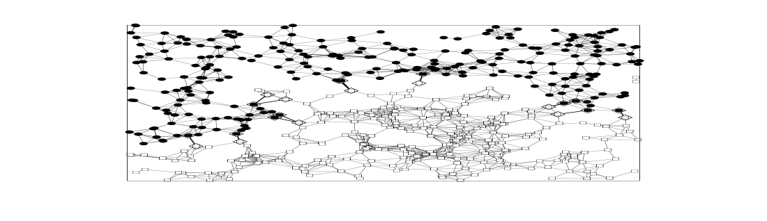
Figure 1: Two random geometric graphs, $N=500$, with connectivities $\alpha\approx 4$ (top) and $\alpha\approx 8$ (bottom) in an optimized configuration found by EO. At $\alpha=4$ the graph barely percolates, with only one “bad” edge connecting the set of 250 round points with the set of 250 square points (diamonds show the two ends of the edge), thus $m_{\rm opt}=1$. For the denser graph on the bottom, EO obtained the cutsize $m_{\rm opt}=13$.

Species in the Bak-Sneppen model are located on the sites of a lattice, and each is represented by a value between 0 and 1 indicating its “fitness”. At each update step, the smallest value (representing the worst adapted species) is discarded and replaced with a new value drawn randomly from a flat distribution on $[0,1]$. Without any interactions, all the fitnesses in the system would eventually become 1. But obvious interdependencies between species provide constraints for balancing the system’s overall fitness with that of its members: the change in fitness of one species impacts the fitness of an interrelated species. Therefore, at each update step in the Bak-Sneppen model, the fitness values on the sites neighboring the smallest value are replaced with new random numbers as well. No explicit definition is given of the mechanism by which these neighboring species are related. Yet after a certain number of updates, the system organizes itself into a highly correlated state known as self-organized criticality (SOC) (Bak 1987). In that state, almost all species have reached a fitness above a certain threshold. But these also species possess what is called punctuated equilibrium (Gould 1977): since one’s weakened neighbor can undermine one’s own fitness, co-evolutionary activity gives rise to chain reactions. Fluctuations that rearrange the fitness of many species occur routinely. These fluctuations can be of the scale of the system itself, making any possible configuration accessible.

In the Bak-Sneppen model, the high degree of adaptation of most species is obtained by the elimination of badly adapted ones instead of a particular “engineering” of better ones. While such dynamics might not lead to as optimal a solution as could be engineered in specific circumstances, it provides near-optimal solutions with a high degree of latency for a rapid adaptation response to changes in the resources that drive the system.

In the following we will describe an optimization method inspired by these insights (Boettcher, submitted, and Boettcher, to appear), called extremal optimization, and study its performance for graph partitioning and the traveling salesman problem.

2 Extremal Optimization and Graph Partitioning

In graph (bi-)partitioning, we are given a set of $N$ points, where $N$ is even, and “edges” connecting certain pairs of points. The problem is to partition the points into two equal subsets, each of size $N/2$, with a minimal number of edges cutting across the partition. (Call the number of these edges the “cutsize” $m$, and the optimal cutsize $m=m_{\rm opt}$.) The points themselves could, for instance, be associated with positions in the unit square. A “geometric” graph of average connectivity $\alpha$ would then be formed by connecting any two points within Euclidean distance $d$, where $N\pi d^{2}=\alpha$ (see Fig. 1). Constraining the partitioned subsets to be of fixed (equal) size makes the solution to the problem particularly difficult. This geometric problem resembles those found in VLSI design, concerning the optimal partitioning of gates between integrated circuits (Dunlop 1985).

Graph partitioning is an NP-hard optimization problem (Garey 1979): it is believed that for large $N$ the number of steps necessary for an algorithm to find the exact optimum must, in general, grow faster than any polynomial in $N$. In practice, however, the goal is usually to find near-optimal solutions quickly. Special-purpose heuristics to find approximate solutions to specific NP-hard problems abound (Alpert 1995, Johnson 1997). Alternatively, general-purpose optimization approaches based on stochastic procedures have been proposed, most notably simulated annealing (Kirkpatrick 1983, Černy 1985) and genetic algorithms (Holland 1975). These methods, although slower, are applicable to problems for which no specialized heuristic exists. Extremal optimization (EO) falls into the latter category, adaptable to a wide range of combinatorial optimizations problems rather than crafted for a specific application.

In close analogy to the Bak-Sneppen model of SOC, the EO algorithm proceeds as follows for the case of graph bi-partitioning:

1. Initially, partition the $N$ points at will into two equal subsets.

2. Rank each point $i$ according to its fitness, $\lambda_{i}=g_{i}/(g_{i}+b_{i})$, where $g_{i}$ is the number of (good) edges connecting $i$ to points within the same subset, and $b_{i}$ is the number of (bad) edges connecting $i$ to the other subset. If point $i$ has no connections at all ($g_{i}=b_{i}=0$), let $\lambda_{i}=1$.

3. Pick the least fit point, i.e., the point (from either subset) with the smallest $\lambda_{i}\in[0,1]$. Pick a second point at random from the other subset, and interchange these two points so that each one is in the opposite subset from where it started.

4. Repeat at (2) for a preset number of times [assume $O(N)$ updates].

The result of an EO run is defined as the best (minimum cutsize) configuration seen so far. All that is necessary to keep track of, then, is the current configuration and the best so far.

EO, like simulated annealing (SA) and genetic algorithms (GA), is inspired by observations of physical systems [for a comparison of SA and GA, see e. g. (de Groot 1991)]. However, SA emulates the behavior of frustrated systems in thermal equilibrium: if one couples such a system to a heat bath of adjustable temperature, by cooling the system slowly one may come close to attaining a state of minimal energy. SA accepts or rejects local changes to a configuration according to the Metropolis algorithm (Metropolis 1953) at a given temperature, enforcing equilibrium dynamics (“detailed balance”) and requiring a carefully tuned “temperature schedule”. In contrast, EO takes the system far from equilibrium: it applies no decision criteria, and all new configurations are accepted indiscriminately. It may appear that EO’s results would resemble an ineffective random search. But in fact, by persistent selection against the worst fitnesses, one quickly approaches near-optimal solutions. At the same time, significant fluctuations still remain at late run-times (unlike in SA), crossing sizable barriers to access new regions in configuration space, as shown in Fig. 2. EO and genetic algorithms are equally contrasted. GAs keep track of entire “gene pools” of solutions from which to select and “breed” an improved generation of global approximations. By comparison, EO operates only with local updates on a single copy of the system, with improvements achieved instead by elimination of the bad.

Figure 2: Evolution of the cutsize during an extremal optimization run on an $N=500$ geometric graph with $\alpha=5$ (see Fig. 1). The shaded area marks the range of cutsizes explored in the respective time bins. The best cutsize ever found is 2, which is visited repeatedly in this run. In contrast to simulated annealing, which has large fluctuations in early stages of the run and then converges much later, extremal optimization quickly approaches a stage where broadly distributed fluctuations allow it to probe many local optima. In this run, a random initial partition was used, and the runtime on a 200MHz Pentium was 9sec.

Further improvements may be obtained through a slight modification of the EO procedure. Step (2) of the algorithm establishes a fitness rank for all points, going from rank $n=1$ for the worst fitness $\lambda$ to rank $n=N$ for the best. (For points with degenerate values of $\lambda$, the ranks may be assigned in random order.) Now relax step (3) so that the points to be interchanged are both chosen from a probability distribution over the rank order: from each subset, we pick a point having rank $n$ with probability $P(n)\propto n^{-\tau},~{}1\leq n\leq N$. The choice of a power-law distribution for $P(n)$ ensures that no regime of fitness gets excluded from further evolution, since $P(n)$ varies in a gradual, scale-free manner over rank. Universally, for a wide range of graphs, we obtain best results for $\tau\approx 1.2-1.6$. What is the physical meaning of an optimal value for $\tau$? If $\tau$ is too small, we often dislodge already well-adapted points of high rank: “good” results get destroyed too frequently and the progress of the search becomes undirected. On the other hand, if $\tau$ is too large, the process approaches a deterministic local search and gets stuck near a local optimum of poor quality. At the optimal value of $\tau$, the more fit components of the solution are allowed to survive, without the search being too narrow. Our numerical studies have indicated that the best choice for $\tau$ is closely related to a transition from ergodic to non-ergodic behavior, with optimal performance of EO obtained near the edge of ergodicity.

To evaluate EO, we tested the algorithm on a testbed of well-studied large graphs discussed in (Hendrickson 1996, Merz 1998). Table 1 summarizes EO’s results on these, using 30 runs of at most $200N$ update steps (in several cases far fewer were necessary; see below). On the first four large graphs, SA’s performance is extremely poor; we therefore substitute results given in (Hendrickson 1996) using a variety of specialized heuristics. EO significantly improves upon these cutsizes, though at longer runtimes. The best results to date on the graphs are due to various GAs (Merz 1998). EO reproduces all of these cutsizes, displaying an increasing runtime advantage as $N$ increases. On the final four graphs, for which no GA results were available, EO matches or dramatically improves upon SA’s cutsizes. And although increasing $\alpha$ generally slows down EO and speeds up SA, EO’s runtime is still nearly competitive with SA’s on the high-connectivity Nasa graphs.

Several factors account for EO’s speed. First of all, in step (1) we employ a simple “greedy” start to form the initial partition, clustering connected points into the same partition from a random seed. This helps EO to succeed rapidly. By contrast, greedy initialization improves the performance of SA only for the smallest and sparsest graphs. Second of all, in step (2) we use a stochastic sorting process to accelerate the algorithm. At each update step, instead of perfectly ordering the fitnesses $\lambda_{i}$, we arrange them on an ordered binary tree called a “heap”. We then select members from the heap such that on average, the actual rank selection approximates $P(n)\sim n^{-\tau}$. This stochastic rank sorting introduces a runtime factor of only $\alpha\log{N}$ per update step. Finally, EO requires significantly fewer update steps (Fig. 2) than, say, a complete SA temperature schedule. The quality of our large $N$ results confirms that $O(N)$ update steps are indeed sufficient for convergence. In the case of the Nasa graphs, only $30N$ update steps (rather than the full $200N$) were in fact required for EO to reach its best results, and in the case of the Brack2 graph, only $2N$ steps were required.

Table 1: Best cutsizes and runtimes for our testbed of graphs. EO and SA results are from our runs (SA parameters as determined by Johnson et al. (Johnson 1989)), using a 200MHz Pentium. GA results are from Merz and Freisleben (Merz 1998), using a 300MHz Pentium. Comparison data for three of the large graphs are due to results from heuristics by Hendrickson (Hendrickson 1996), using a 50MHz Sparc20.

Graph	EO		GA		heuristics
Hammond	90	(42s)	90	(1s)	97	(8s)
($N=4720$; $\alpha=5.8$)
Barth5	139	(64s)	139	(44s)	146	(28s)
($N=15606$; $\alpha=5.8$)
Brack2	731	(12s)	731	(255s)	—
($N=62632$; $\alpha=11.7$)
Ocean	464	(200s)	464	(1200s)	499	(38s)
($N=143437$; $\alpha=5.7$)
Graph			EO		SA
Nasa1824			739	(6s)	739	(3s)
($N=1824$; $\alpha=20.5$)
Nasa2146			870	(10s)	870	(2s)
($N=2146$; $\alpha=32.7$)
Nasa4704			1292	(15s)	1292	(13s)
($N=4704$; $\alpha=21.3$)
Stufe10			51	(180s)	371	(200s)
($N=24010$; $\alpha=3.8$)

3 Optimizing near Critical Points

Further comparison of EO and SA, averaged over a large sample of a particular type of graph, shows EO to be especially useful near critical points (Boettcher, to appear). It has been observed that many optimization problems exhibit critical points delimiting “easy” phases of a generally hard problem (Cheeseman 1991). Near such a critical point, finding solutions becomes particularly difficult for local search methods that explore some neighborhood in configuration space starting from an existing state. Near-optimal solutions become widely separated with diverging barrier heights between them. It is not surprising that equilibrium search methods based on heat-bath techniques like SA are not particularly successful here (Binder 1987). In contrast, the driven dynamics of EO does not possess any temperature control parameters that could increasingly limit the scale of fluctuations. A non-equilibrium approach like EO thus provides a general-purpose optimization method that is complementary to SA, which would be expected to freeze quickly into a poor local optimum “where the really hard problems are” (Cheeseman 1991).

Figure 3: Plot of SA’s error relative to the best result found on geometric graphs, as a function of the mean connectivity $\alpha$.

Figure 4: Scaling plot of the data from EO according to Eq. 1 for geometric graphs, as a function of the mean connectivity $\alpha$. The scaling parameters and the fit are as discussed in the text.

As an example, we explore this critical point for the equal partitioning of geometric graphs, as a function of their connectivity. It is hopeless to obtain reliable benchmarks for the exact optimal partition of large graphs. Instead, by averaging over many instances we can try to reproduce well-known results from the percolation properties of this class of graphs. For instance, when the average connectivity $\alpha$ of a geometric graph is much below $\alpha_{\rm crit}\approx 4.5$, the percolation threshold found for these graphs (Balberg 1985), the graph most likely consists of many small clusters. These can easily be sorted into equal sized partitions with vanishing cutsize, at a cost of at most O($N^{2}$). When, on the other hand, the connectivity is large, the graph is dense and almost homogeneous with many near-optimal solutions in close proximity. But for connectivities near $\alpha_{\rm crit}$, a “percolating” cluster of size O($N$) appears with very widely separated minima (see Fig. 1), making both the decision problem and the actual search very costly (Cheeseman 1991).

We have generated geometric graphs of connectivities between $\alpha=4$ and $\alpha=10$ (by varying the threshold distance $d$ below which points are connected), at $N=500$, 1000, 2000, 4000, 8000, and 16000. For each $\alpha$ we generated 16 different instances of graphs, identical for SA and EO. We performed 32 optimization runs for each method on each instance. On each run, we used a different random seed to establish an initial partition of the points. SA was run using the algorithm developed by Johnson et al. (Johnson 1989) for this case, but with a temperature length four times longer, to improve results. EO was run for $200N$ update steps to produce a comparable runtime. For each method, we have taken only the best result from all runs on a given instance. We average those best results, for a particular connectivity $\alpha$, to obtain the mean cutsize for that method as a function of $\alpha$ and $N$. To compare EO and SA, we determine the relative error of SA with respect to the best result found by either method (most often by EO!) for $\alpha\geq\alpha_{\rm crit}$. Fig. 3 suggests that the error of SA diverges about linearly with increasing $N$, near $\alpha_{\rm crit}$.

For the data obtained with EO, we make an Ansatz

$$\langle m_{\rm opt}\rangle\sim N^{\nu}\left(\alpha-\alpha_{\rm 0}\right)^{\beta}$$ (1)

with $\nu=0.6$, in order to scale the data for all $N$ onto a single curve (see Fig. 4). The remaining parameters are established according to a data fit, yielding $\alpha_{0}=4.1$ and $\beta=1.4$. The fact that $\alpha_{0}<\alpha_{\rm crit}$ indicates that below the percolation threshold EO’s cutsizes are already non-vanishing, and so even EO does not always find optimal partitions there.

4 Extremal Optimization of the TSP

In the graph partitioning problem, the implementation of EO is particularly straightforward. The concept of fitness, however, is equally meaningful in any optimization problem whose cost function can be decomposed into $N$ equivalent degrees of freedom. Thus, EO may be applied to many other NP-hard problems, even those where the choice of quantities for the fitness function, as well as the choice of elementary move, is less clear than in graph partitioning. One case where these choices are far from obvious is the traveling salesman problem. Even so, we have found there that EO presents a challenge to more finely tuned methods (Boettcher, submitted).

In the traveling salesman problem (TSP), $N$ points (“cities”) are given, and every pair of cities $i$ and $j$ is separated by a distance $d_{ij}$. The problem is to connect the cities using the shortest closed “tour”, passing through each city exactly once. For our purposes, take the $N\times N$ distance matrix $d_{ij}$ to be symmetric. Its entries could be the Euclidean distances between cities in a plane — or alternatively, random numbers drawn from some distribution, making the problem non-Euclidean. (The former case might correspond to a business traveler trying to minimize driving time; the latter to a traveler trying to minimize expenses on a string of airline flights, whose prices certainly do not obey triangle inequalities!)

For the TSP, we implement EO in the following way. Consider each city $i$ as a degree of freedom, with a fitness based on the two links emerging from it. Ideally, a city would want to be connected to its first and second nearest neighbor, but is often “frustrated” by the competition of other cities, causing it to be connected instead to (say) its $p$th and $q$th neighbors, $1\leq p\neq q\leq N-1$. Let us define the fitness of city $i$ to be $\lambda_{i}=3/(p_{i}+q_{i})$, so that $\lambda_{i}=1$ in the ideal case.

Defining a move class (step (3) in EO’s algorithm) is more difficult for the TSP than for graph partitioning, since the constraint of a closed tour requires an update procedure that changes several links at once. One possibility, used by SA among other local search methods, is a “two-change” rearrangement of a pair of non-adjacent segments in an existing tour. There are $O(N^{2})$ possible choices for a two-change. Most of these, however, lead to even worse results. For EO, it would not be sufficient to select two independent cities of poor fitness from the rank list, as the resulting two-change would destroy more good links than it creates. Instead, let us select one city $i$ according to its fitness rank $n_{i}$, using the distribution $P(n)\sim n^{-\tau}$ as before, and eliminate the longer of the two links emerging from it. Then, reconnect $i$ to a close neighbor, using the same distribution function $P(n)$ as for the rank list of fitnesses, but now applied instead to a rank list of $i$’s neighbors ($n=1$ for first neighbor, $n=2$ for second neighbor, and so on). Finally, to form a valid closed tour, one of the old links to the new (neighbor) city must be replaced; there is a unique way of doing so. For the optimal choice of $\tau$, this move class allows us the opportunity to produce many good neighborhood connections, while maintaining enough fluctuations to explore the configuration space.

Table 2: Best tour-lengths found for the Euclidean (top) and the random-distance TSP (bottom). Results for each value of $N$ are averaged over 10 instances, using on each instance an exact algorithm (except for $N=256$ Euclidean where none was available), the best-of-ten EO runs, and the best-of-ten SA runs. Euclidean tour-lengths are rescaled by $1/\sqrt{N}$.

$N$	Exact	EO10	SA10
Euclidean  16	0.71453	0.71453	0.71453
32	0.72185	0.72237	0.72185
64	0.72476	0.72749	0.72648
128	0.72024	0.72792	0.72395
256	—	0.72707	0.71854
Rand. Dist.  16	1.9368	1.9368	1.9368
32	2.1941	2.1989	2.1953
64	2.0771	2.0915	2.1656
128	2.0097	2.0728	2.3451
256	2.0625	2.1912	2.7803

We performed simulations at $N=16$, 32, 64, 128, and 256, in each case generating ten random instances for both the Euclidean and non-Euclidean TSP. The Euclidean case consisted of $N$ points placed at random in the unit square with periodic boundary conditions; the non-Euclidean case consisted of a symmetric $N\times N$ distance matrix with elements drawn randomly from a uniform distribution on the unit interval. On each instance we ran both EO and SA, selecting for both methods the best of 10 runs from random initial conditions. EO used $\tau=4$ (Eucl.) and $\tau=4.4$ (non-Eucl.), with $16N^{2}$ update steps. SA used an annealing schedule with $\Delta T/T=0.9$ and temperature length $32N^{2}$. The results are given in Table 2, along with baseline results using an exact algorithm. While the EO results trail those of SA by up to about 1% in the Euclidean case, EO significantly outperforms SA for the non-Euclidean (random distance) TSP. Surprisingly, using increased run times (longer temperature schedules) diminishes rather than improves SA’s performance in the latter case. Finally, note that one would not expect a general method such as EO to be competitive here with specialized optimization algorithms designed particularly with the TSP in mind. But remarkably, EO’s performance in both the Euclidean and non-Euclidean cases — within several percent of optimality for $N\leq 256$ — places it not far behind the leading specially-crafted TSP heuristics (Johnson 1997).

5 Extremal Optimization and Learning

Our results therefore indicate that a simple extremal optimization approach based on self-organizing dynamics can outperform state-of-the-art (and far more complicated or finely tuned) general-purpose algorithms on hard optimization problems. Based on its success on the generic and broadly applicable graph partitioning problem, as well as on the TSP, we believe the concept will be applicable to numerous other NP-hard problems. It is worth stressing that the rank ordering approach employed by EO is inherently non-equilibrium. Such an approach could not, for instance, be used to enhance SA, whose temperature schedule requires equilibrium conditions. This rank ordering serves as a sort of “memory”, allowing EO to retain well-adapted pieces of a solution. In this respect it mirrors one of the crucial properties noted in the Bak-Sneppen model (Boettcher 1996). At the same time, EO maintains enough flexibility to explore further reaches of the configuration space and to “change its mind”. Its success at this complex task provides motivation for the use of extremal dynamics to model mechanisms such as learning, as has been suggested recently to explain the high degree of adaptation observed in the brain (Chialvo 1999).

References

C. J. Alpert and A. B. Kahng, Integration: the VLSI Journal 19, 1 (1995).

P. Bak, How Nature Works (Springer, New York, 1996).

P. Bak, C. Tang, and K. Wiesenfeld, Phys. Rev. Lett. 59, 381 (1987).

P. Bak and K. Sneppen, Phys. Rev. Lett. 71, 4083 (1993).

I. Balberg, Phys. Rev. B 31, R4053 (1985).

K. Binder, Applications of the Monte Carlo Method in Statistical Physics, K. Binder, Ed. (Springer, Berlin, 1987).

S. Boettcher and M. Paczuski, Phys. Rev. E 54, 1082 (1996), and Phys. Rev. Lett. 79, 889 (1997).

S. Boettcher, J. Phys. A: Math. Gen, to appear; available at http://xxx.lanl.gov/abs/cond-mat/9901353.

S. Boettcher and A. G. Percus, submitted to Artificial Intelligence; available at http://xxx.lanl.gov/abs/cond-mat/9901351.

V. Černy, J. Optimization Theory Appl. 45, 41 (1985).

P. Cheeseman, B. Kanefsky, and W. M. Taylor, in Proc. of IJCAI-91, J. Mylopoulos and R. Rediter, Eds. (Morgan Kaufmann, San Mateo, CA, 1991), pp. 331–337.

D. R. Chialvo and P. Bak, J. Neurosci., to appear.

C. Darwin, The Origin of Species by Means of Natural Selection (Murray, London, 1859).

A. E. Dunlop and B. W. Kernighan, IEEE Trans. on Computer-Aided Design CAD–4, 92 (1985).

M. R. Garey and D. S. Johnson, Computers and Intractability: A Guide to the Theory of NP-Completeness (Freeman, New York, 1979).

S. J. Gould and N. Eldridge, Paleobiology 3, 115–151 (1977).

C. de Groot, D. Wuertz, K. H. Hoffmann, Lecture Notes in Computer Science 496, 445-454 (1991).

B. A. Hendrickson and R. Leland, in Proceedings of the 1995 ACM/IEEE Supercomputing Conference (Supercomputing ’95), San Diego, CA, December 3–8, 1995 (ACM Press, New York, 1996).

J. Holland, Adaptation in Natural and Artificial Systems (University of Michigan Press, Ann Arbor, 1975).

D. S. Johnson, C. R. Aragon, L. A. McGeoch, and C. Schevon, Operations Research 37, 865 (1989).

D. S. Johnson and L. A. McGeoch, in Local Search in Combinatorial Optimization, E. H. L. Aarts and J. K. Lenstra, Eds. (Wiley, New York, 1997), chap. 8.

S. Kirkpatrick, C. D. Gelatt, and M. P. Vecchi, Science 220, 671 (1983).

B. B. Mandelbrot, The Fractal Geometry of Nature (Freeman, New York, 1983).

P. Merz and B. Freisleben, in Lecture Notes in Computer Science: Parallel Problem Solving From Nature — PPSN V, A. E. Eiben, T. Bäck, M. Schoenauer, and H.-P. Schwefel, Eds. (Springer, Berlin, 1998), vol. 1498, pp. 765–774, and Technical Report No. TR–98–01 (Department of Electrical Engineering and Computer Science, University of Siegen, Siegen, Germany, 1998), available at http://www.informatik.uni-siegen.de/~pmerz/publications.html.

N. Metropolis, A. W. Rosenbluth, M. N. Rosenbluth, A. H. Teller, and E. Teller, J. Chem. Phys. 21, 1087 (1953).

M. Paczuski, S. Maslov, and P. Bak, Phys. Rev. E 53, 414 (1996).

I. Rodriguez-Iturbe and A. Rinaldo, Fractal River Basins: Chance and Self-Organization (Cambridge, New York, 1997).

K. Sneppen, P. Bak, H. Flyvbjerg, and M. H. Jensen, Proc. Natl. Acad. Sci. 92, 5209 (1995).