Geometric Knot Spaces and Polygonal Isotopy

Abstract.

The space of $n$-sided polygons embedded in three-space consists of a smooth manifold in which points correspond to piecewise linear or “geometric” knots, while paths correspond to isotopies which preserve the geometric structure of these knots. The topology of these spaces for the case $n=6$ and $n=7$ is described. In both of these cases, each knot space consists of five components, but contains only three (when $n=6$) or four (when $n=7$) topological knot types. Therefore “geometric knot equivalence” is strictly stronger than topological equivalence. This point is demonstrated by the hexagonal trefoils and heptagonal figure-eight knots, which, unlike their topological counterparts, are not reversible. Extending these results to the cases $n\geq 8$ will also be discussed.

Keywords: polygonal knots, space polygons, knot spaces, knot invariants.

1. Introduction

Consider the sorts of configurations that can be constructed out of a sequence of line segments, glued end to end to end to form an embedded loop in $\mathbb{R}^{3}.$ The line segments might represent bonds between atoms in a polymer, segments in the base-pair sequence of a circular DNA macromolecule, or simply thin wooden sticks attached with flexible rubber joints. Thus, a spatial polygon of this kind serves as a mathematical model for some object which is physically knotted yet retains some of the rigidity inherited from the materials from which it is built.

It is a classical result of three-dimensional topology that knotted loops made out of flexible string can always be approximated by polygonal loops consisting of many thin, rigid segments. Furthermore, any deformation performed on the string can always be approximated by a deformation of the polygon, as long as the number of edges is allowed to increase. However if we insist that the number of edges remain constant, then we clearly restrict the types of knots that we can construct. For instance, if we use five or fewer edges, every loop we build is topologically unknotted; on the other hand we can build a trefoil or a figure-eight knot if we use six or seven edges, respectively. See Figure  1. What is not clear is whether we can always mimic a topological deformation by a deformation of polygons when we place restrictions on the number of edges. For instance, it is unknown whether we can build a really complicated polygon which, if it were made out of flexible string, could be topologically deformed into a round unknot but, if it were built out of rigid sticks with flexible joints, could not be flattened out into a planar polygon. In other words, it is an open question whether there exist topological unknots which are geometrically knotted.

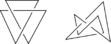
Figure 1. A hexagonal trefoil knot and a heptagonal figure-eight knot.

As it turns out, it is not always possible to find a geometric isotopy (i.e. one which keeps the number of edges fixed) between two polygonal configurations which are topologically equivalent. In fact, even the case of hexagonal trefoils is nontrivial, as there are distinct geometric isotopy types, or isotopes, of this knot. As a consequence, familiar properties such as reversibility behave differently when dealing with geometric knots.

One formulation due to Dick Randell [13, 14] is obtained by observing the correspondence between $n$-sided polygonal loops in Euclidean three-space and points in $\mathbb{R}^{3n}.$ Suppose that $P$ is an $n$-sided polygon in $\mathbb{R}^{3},$ together with a choice of a “first vertex” $v_{1}$ and an orientation. By listing the coordinates of each vertex in sequence, we obtain a point $(x_{1},y_{1},z_{1},x_{2},y_{2},z_{2},\ldots,x_{n},y_{n},z_{n})\in\mathbb{R}^{3n}$ which we associate with $P=\langle v_{1},v_{2},\ldots,v_{n}\rangle.$ As in the theory of Vassiliev invariants, let the discriminant $\Sigma^{(n)}$ be the set of all points in $\mathbb{R}^{3n}$ which correspond to polygons with self-intersections. If $n>3,$ this discriminant is the union of $\frac{1}{2}n(n-3)$ pieces, each of which corresponds to the set of polygons with an intersecting pair of non-adjacent edges. For instance, the subset in $\Sigma^{(n)}$ consisting of polygons for which the edges $v_{1}v_{2}$ and $v_{3}v_{4}$ intersect can be described as the collection of polygons for which:

1. the vertices $v_{1},v_{2},v_{3},$ and $v_{4}$ are coplanar,

2. the line determined by $v_{1}$ and $v_{2}$ separates $v_{3}$ from $v_{4},$ and

3. the line determined by $v_{3}$ and $v_{4}$ separates $v_{1}$ from $v_{2}.$

Note that this set corresponds to the closure of the locus in $\mathbb{R}^{3n}$ of the system

$$(v_{2}-v_{1})\times(v_{3}-v_{1})\cdot(v_{4}-v_{1})=0,$$

$$(v_{2}-v_{1})\times(v_{3}-v_{1})\cdot(v_{2}-v_{1})\times(v_{4}-v_{1})<0,$$

$$(v_{4}-v_{3})\times(v_{1}-v_{3})\cdot(v_{4}-v_{3})\times(v_{2}-v_{3})<0.$$

Therefore, each of these pieces is the closure of a codimension one cubic semi-algebraic variety, i.e. a hypersurface with boundary. We define the space of geometric knots to be the complement of this discriminant, $\mathfrak{Geo}^{(n)}=\mathbb{R}^{3n}-\Sigma^{(n)}.$ Therefore $\mathfrak{Geo}^{(n)}$ is a dense open submanifold of $\mathbb{R}^{3n}.$ In this space, points correspond to embedded polygons or geometric knots, paths correspond to geometric isotopies, and path-components correspond to geometric knot types.

By a theorem of Whitney [18], for any given $n$ there are only finitely many path-components in $\mathfrak{Geo}^{(n)}.$ It is also a well-known “folk theorem,” due perhaps to Kuiper, that the spaces $\mathfrak{Geo}^{(3)},\mathfrak{Geo}^{(4)},$ and $\mathfrak{Geo}^{(5)}$ are connected. In [2, 3], I showed that the spaces $\mathfrak{Geo}^{(6)}$ and $\mathfrak{Geo}^{(7)}$ have five components each. Contrast this with the fact that only three topological knot types are represented in $\mathfrak{Geo}^{(6)},$ and that only four topological knot types are present in $\mathfrak{Geo}^{(7)}.$ When $n>8,$ the exact number of path-components remains unknown. In fact, even the number of topological knot types represented in the different components of $\mathfrak{Geo}^{(n)}$ is known only when $n<9.$ The following theorem summarizes the current status of the classification of geometric knots with a small number of edges.

Theorem 1.

(Calvo [2, 3])

1. The spaces $\mathfrak{Geo}^{(3)},\mathfrak{Geo}^{(4)},$ and $\mathfrak{Geo}^{(5)}$ are path-connected and consist only of unknots.

2. The space $\mathfrak{Geo}^{(6)}$ of hexagonal knots contains five path-components. These consist of a single component of unknots, two components of right-handed trefoils, and two components of left-handed trefoils.

3. The space $\mathfrak{Geo}^{(7)}$ of heptagonal knots contains five path-components. These consist of a single component of unknots and of each type of trefoil knot, and two components of figure-eight knots.

4. The space $\mathfrak{Geo}^{(8)}$ of octagonal knots contains at least twenty path-components. However, the only knots represented in this space are the unknot, the trefoil knot, the figure-eight knot, every five and six crossing prime knot $(5_{1},5_{2},6_{1},6_{2},$ and $6_{3}),$ the square and granny knots $(3_{1}\pm 3_{1}),$ the (3, 4)-torus knot $(8_{19}),$ and the knot $8_{20}.$

It is important to note that although the deformations obtained as paths in $\mathfrak{Geo}^{(n)}$ preserve the polygonal structure of the knot in question, in general they will not preserve edge length. Let $f:\mathfrak{Geo}^{(n)}\rightarrow\mathbb{R}^{n}$ be the map taking $P=\langle v_{1},v_{2},\ldots,v_{n}\rangle$ to the $n$-tuple

$$(\lVert v_{1}-v_{2}\rVert,\lVert v_{2}-v_{3}\rVert,\ldots,\lVert v_{n-1}-v_{n}\rVert,\lVert v_{n}-v_{1}\rVert).$$

Then points in the preimage $\mathfrak{Equ}^{(n)}=f^{-1}(1,1,\ldots,1)$ correspond to equilateral knots with unit length edges. Since the point $(1,1,\ldots,1)$ is a regular value for $f,$ the space $\mathfrak{Equ}^{(n)}$ is a $2n$-dimensional submanifold (in fact, a codimension $n$ quadric hypersurface) intersecting a number of the components of $\mathfrak{Geo}^{(n)},$ some perhaps more than once. Paths in this submanifold correspond to geometric isotopies which do preserve edge length, so the path-components of this space offer yet another notion of knottedness.

In his original papers on molecular conformation spaces [13, 14], Randell shows that if $n\leq 5$ then $\mathfrak{Equ}^{(n)}$ is connected. The case when $n=6$ had virtually remained untouched for ten years, except for work by Kenneth Millett and Rosa Orellana showing that $\mathfrak{Equ}^{(6)}$ contains a single component of topological unknots. ​​ By focusing attention to a special case of singular “almost knotted” hexagons, [3] shows that two hexagons are equilaterally equivalent exactly when they are geometrically equivalent. Thus $\mathfrak{Equ}^{(6)}$ intersects each component of $\mathfrak{Geo}^{(6)}$ exactly once. Furthermore, [3] shows that this correspondence of path-components is not uninteresting, as the inclusion $\mathfrak{Equ}^{(6)}\hookrightarrow\mathfrak{Geo}^{(6)}$ has a nontrivial kernel at the level of fundamental group. In fact, if $\mathcal{T}$ is a component of trefoils in $\mathfrak{Geo}^{(6)},$ then $\pi_{1}(\mathcal{T})=\mathbb{Z}_{2}$ while $\pi_{1}(\mathcal{T}\cap\mathfrak{Equ}^{(6)})$ contains an infinite cyclic subgroup.

This paper presents two key ingredients from [2, 3] used to obtain Theorem 1. In Section 2, we discuss a method of decomposing $\mathfrak{Geo}^{(n)}$ into three-dimensional fibres or “strata.” This method proved particularly useful in the analysis of $\mathfrak{Geo}^{(6)}$ and $\mathfrak{Geo}^{(7)}.$ Then Section  3 describes an upper bound on the minimal crossing number of the knot realized by an $n$-sided polygon. This bound, which is obtained by looking at a particular projection of polygon into a sphere, improves the one previously known by a linear term and provides enough control to classify the topological knot types present in $\mathfrak{Geo}^{(8)}.$

2. A Stratification of Geometric Knot Spaces

Consider the map $g$ with domain $\mathfrak{Geo}^{(n)}$ which “forgets” the last vertex of a polygon, mapping

$$P=\langle v_{1},v_{2},v_{3},\ldots,v_{n-1},v_{n}\rangle\mapsto g(P)=\langle v_{1},v_{2},v_{3},\ldots,v_{n-1}\rangle.$$

Notice that a generic polygon in $\mathfrak{Geo}^{(n)}$ will map to an embedded polygon in $\mathfrak{Geo}^{(n-1)};$ the only polygons which do not are the ones for which some part of the linkage $v_{1}v_{2}\ldots v_{n-1}$ passes through the line segment between $v_{1}$ and $v_{n-1},$ and these polygons form a codimension one subset of $\mathfrak{Geo}^{(n)}.$ In particular, since $\mathfrak{Geo}^{(n)}$ is a manifold, every $n$-sided polygon can be perturbed by just a tiny amount so that its image under $g$ lies in $\mathfrak{Geo}^{(n-1)}.$

Suppose that $Q$ is an $(n-1)$-sided polygon in $\mathfrak{Geo}^{(n-1)}.$ Then the preimage $g^{-1}(Q)$ will be a three-dimensional manifold, homeomorphic to the set of valid $n$th vertices for $Q.$ This divides $\mathfrak{Geo}^{(n)}$ into three-dimensional slices or strata. As $Q$ varies over $\mathfrak{Geo}^{(n-1)},$ the corresponding three-dimensional stratus $g^{-1}(Q)$ will vary. By observing how these strata change, we can obtain useful information about $\mathfrak{Geo}^{(n)}.$

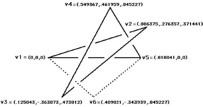
Figure 2. One possible sixth vertex for the pentagon $Q.$

For example, consider the pentagon $Q=\langle v_{1},v_{2},v_{3},v_{4},v_{5}\rangle$ with coordinates

$$\langle(0,0,0),(.886375,.276357,.371441),$$

$$(.125043,-.363873,.473812),$$

$$(.549367,.461959,.845227),(.818041,0,0)\rangle$$

shown in Figure  2. Suppose that we replace the edge between $v_{5}$ and $v_{1}$ with a pair of new edges, from $v_{5}$ to some new vertex $v_{6}\in\mathbb{R}^{3}$ and from this vertex back to $v_{1}.$ This creates a hexagon which, with a bit of care in choosing $v_{6},$ will also be embedded in $\mathbb{R}^{3}.$ For instance, if we place the new vertex at $(.4090205,0,-.912525),$ we obtain an unknotted hexagon. On the other hand, placing $v_{6}$ at $(.4090205,-.343939,.845227),$ gives a hexagon which is knotted as a right-handed trefoil. See Figure  2. The preimage $g^{-1}(Q)\in\mathfrak{Geo}^{(6)}$ is homeomorphic to the dense open subset of $\mathbb{R}^{3}$ consisting of “valid” sixth vertices for $Q.$

To examine which points in $\mathbb{R}^{3}$ correspond to embedded hexagons obtained from $Q,$ we will think of the $x$-axis as a “central axis” in this space and consider the collection of half-planes radiating from this axis. We refer to these as standard half-planes. These half-planes appear as rays from the origin in Figure  3, which shows the projection of $Q$ into the $yz$-plane.

Let $\mathcal{P}_{2},\mathcal{P}_{3},$ and $\mathcal{P}_{4}$ be the standard half-planes containing $v_{2},v_{3},$ and $v_{4},$ respectively. Thus

$$\mathcal{P}_{2}=\{y=\tfrac{276357}{371441}z\approx.744z,\;z>0\},$$

$$\mathcal{P}_{3}=\{y=-\tfrac{363873}{473812}z\approx-.768z,\;z>0\},$$

$$\mathcal{P}_{4}=\{y=\tfrac{461959}{845227}z\approx.547z,\;z>0\},$$

as shown in Figure  3.

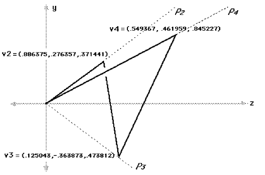
Figure 3. Projection of pentagon $Q$ into $yz$-plane.

Notice that the interior of any standard half-plane to the left of $\mathcal{P}_{2}$ and $\mathcal{P}_{3}$ will miss $Q$ altogether. Thus, any point in the interior of any these half-planes may be used as a sixth vertex for a hexagon. Every other standard half-plane, however, does intersect $Q$ at one or more interior points, so these half-planes will contain some points which correspond to hexagons with self-intersections.

The interior of any standard half-plane between $\mathcal{P}_{2}$ and $\mathcal{P}_{4}$ will intersect $Q$ only once, in its second edge. Depending on which point of this plane we choose for the new vertex $v_{6},$ the two-edge linkage $v_{5}v_{6}v_{1}$ will either dip underneath or jump over this edge. If $v_{5}v_{6}v_{1}$ goes under $v_{2}v_{3},$ then $v_{6}$ can be dragged back to the $x$-axis, say to the midpoint of edge $v_{1}v_{5},$ giving an isotopy of the resulting hexagon back to the unknotted loop realized by the pentagon $Q.$ However, if $v_{5}v_{6}v_{1}$ loops above the edge $v_{2}v_{3},$ then this edge will obstruct any isotopy of the hexagon which attempts to push $v_{6}$ down towards the $x$-axis in this plane. For instance, $Q$ crosses the half-plane $\{y=.6z,\;z>0\}$ at the point $(.828333,.227547,.379246).$ Vertices collinear with $(.828333,.227547,.379246)$ and $v_{1}$ correspond to embedded hexagons only when they lie between these points; otherwise the second and sixth edges of the resulting hexagon will cross each other. Similarly, vertices collinear with $(.828333,.227547,.379246)$ and $v_{5}$ which do not lie between these two points correspond to hexagons with intersecting second and fifth edges. Therefore, points in the rays beginning at $(.828333,.227547,$ $.379246)$ and radiating away from either $v_{1}$ or $v_{5}$ do not correspond to embedded hexagons, and the half-plane is cut into two regions by a “V”-shaped discriminant. See Figure  4(a). If $v_{6}$ is placed in the region of this half-plane labelled i, then the pair of new edges will dip under the edge $v_{2}v_{3}$ and the resulting hexagon will be isotopic to $Q.$ Alternatively, if $v_{6}$ is placed in the region labelled ii, then $v_{5}v_{6}v_{1}$ will jump over this edge.

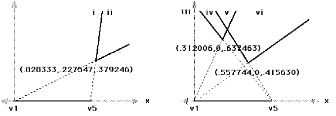
(a) $\{y=.6z,\;z>0\}$                                              (b) $\{y=0,\;z>0\}$     

Figure 4. $Q$ separates each half-plane by “V”-shaped discriminants.

Now, the interior of every standard half-plane between $\mathcal{P}_{4}$ and $\mathcal{P}_{3}$ intersects $Q$ in two points, in the interior of its second and third edges. As before, these edges will form obstructions to a homotopy moving $v_{6}$ in this plane. Therefore, for each of the points through which these edges cross the half-plane, there will be a “V”-shaped discriminant as above. For example, in the half-plane $\{y=0,\;z>0\},$ which intersects $Q$ at the points $(.557744,0,.415630)$ and $(.312006,0,.637463),$ vertices in the four rays beginning at either of these points and radiating away from $v_{1}$ and $v_{5}$ correspond to hexagons with self-intersections. These two “V”-shaped discriminants separate the half-plane into four regions, arranged as in Figure  4(b). As before, placing the new vertex in each of these regions corresponds to looping the new edges of the hexagon over either the second (vi) or third (iv) edge of $Q,$ or both (v), or neither (iii) of these.

We can show that the arrangement of the “V”-shaped discriminants remains relatively unchanged for standard half-planes in each of these intervals. In fact, the connected components of the half-planes in Figure  4 are only cross-sectional slices of “cylindrical sectors” of $g^{-1}(Q)$ which wrap around the $x$-axis. Denote these sectors as i, ii, iii, iv, v, and vi, using the notation in Figure  4. Furthermore, let o denote the sector of $g^{-1}(Q)$ corresponding to vertices in half-planes which do not intersect $Q$ at all. Then the way in which these sectors are glued together depends on the behavior of the discriminants at the three “critical level” standard half-planes $\mathcal{P}_{2},\mathcal{P}_{3},$ and $\mathcal{P}_{4}.$

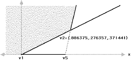
Figure 5. Critical level $\mathcal{P}_{2}=\{y=\tfrac{276357}{371441}z\approx.744z,\;z>0\}.$

The first of these half-planes, $\mathcal{P}_{2},$ contains the first edge of $Q,$ which connects $v_{1}=(0,0,0)$ to $v_{2}=(.886375,.276357,.371441).$ Vertices in rays beginning at any point in this edge and radiating away from $v_{6}$ correspond to hexagons with intersecting first and fifth edges. Hence, for each point in this edge there is a “V”-shaped discriminant. The union of these discriminants forms a two-dimensional discriminant corresponding to an obstruction in the space $g^{-1}(Q).$ See Figure  5. However, this obstruction only partially blocks access to sector i. Therefore both i and ii are glued to o at this half-plane.

A similar two-dimensional discriminant occurs for $\mathcal{P}_{4}.$ This half-plane contains the fourth edge of $Q,$ which joins $v_{4}=(.549367,.461959,.845227)$ and $v_{5}=(.818041,$ $0,0).$ Vertices collinear with the origin and any point $p$ on this edge correspond to embedded hexagons only if they lie between $(0,0,0)$ and $p.$ See Figure  6. This discriminant completely closes off sector vi, and obstructs parts of sectors i, ii, and iii. Thus, at this level, i is attached to iii and iv, ii is attached to v, and vi is abruptly terminated.

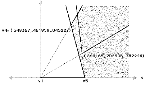
Figure 6. Critical level $\mathcal{P}_{4}=\{y=\tfrac{461959}{845227}z\approx.547z,\;z>0\}.$

The third critical level half-plane, $\mathcal{P}_{3},$ presents a different situation, as it intersects $Q$ only at the vertex $v_{3}=(.125043,-.363873,.473812).$ In this case, the “V”-shaped discriminants corresponding to the second and third edges of $Q$ come together as the two edges become incident at their common vertex. As the discriminants merge, sectors iv and vi are terminated, while both of the sectors iii and v merge with sector o.

Figure  7 presents a cylindrical section of $\mathbb{R}^{3}$ about the $x$-axis, showing the sectors of $g^{-1}(Q)$ and the connections between them. In particular, it shows that $g^{-1}(Q)$ consists of two disjoint path-components, corresponding to the two knot types possible for hexagons in the stratus $g^{-1}(Q)$: the unknot and the right-handed trefoil.

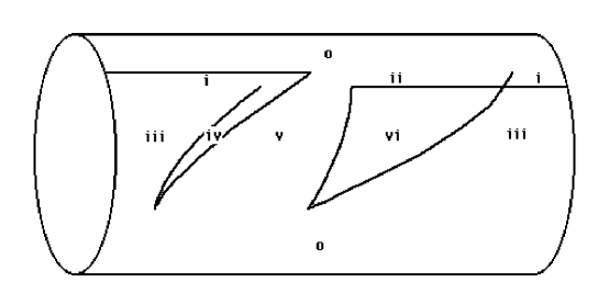
Figure 7. Cylindrical section of $\mathbb{R}^{3}$ showing the different interconnecting sectors of $g^{-1}(Q).$

The key feature characterizing a pentagon’s corresponding stratus in $\mathfrak{Geo}^{(6)}$ is the relative position of the second, third, and fourth vertices with respect to the axis through the other two vertices. Suppose that $Q=\langle v_{1},v_{2},v_{3},v_{4},v_{5}\rangle$ is an arbitrary pentagon in $\mathfrak{Geo}^{(5)},$ and that $\mathcal{L}$ is the line determined by $v_{1}$ and $v_{5}.$ Since $\mathfrak{Geo}^{(5)}$ is a manifold, we can perturb $Q$ slightly, if necessary, to ensure that $v_{1}v_{5}$ is the only edge of $Q$ which intersects $\mathcal{L}.$ As above, let $\mathcal{P}_{2},\mathcal{P}_{3},$ and $\mathcal{P}_{4}$ be the half-planes with boundary $\mathcal{L}$ which contain $v_{2},v_{3},$ and $v_{4},$ respectively. Again, a slight deformation will make $Q$ a generic pentagon, guaranteeing that the three $\mathcal{P}_{i}$’s are distinct.

As in the example above, the $\mathcal{P}_{i}$’s will divide $\mathbb{R}^{3}$ into three open regions, with $Q$ intersecting two of these and completely missing the third. As we rotate in a right-handed fashion about the axis $\mathcal{L},$ beginning in the region which misses $Q,$ we will encounter each of the $\mathcal{P}_{i}$’s in one of six orders. For example, in the pentagon shown in Figures  2 and 3, these half-planes appear in the order $\mathcal{P}_{2}-\mathcal{P}_{4}-\mathcal{P}_{3},$ or simply, 2-4-3.

Let $H\in\mathfrak{Geo}^{(6)}$ be a generic hexagon embedded in $\mathbb{R}^{3}.$ By considering the order in which the $\mathcal{P}_{i}$’s associated with $g(H)$ occur, we divide $\mathfrak{Geo}^{(6)}$ into six open regions meeting along codimension one sets where either:

1. two of the $\mathcal{P}_{i}$’s coincide, or

2. an edge of $H$ crosses $\mathcal{L}.$

By analyzing the behavior of the strata $g^{-1}(g(H))$ as they interconnect, we obtain Table  1, which indicates the number of path-components in each of the six regions of $\mathfrak{Geo}^{(6)},$ arranged by the topological knot type they represent.

Table 1. Number of components in each region of $\mathfrak{Geo}^{(6)}.$

$\mathbf{Region\,of\,\mathfrak{Geo}^{(6)}}$		$\quad\mathbf{0}\quad$	$\quad\mathbf{3_{1}}\quad$	$\;\,\mathbf{-3_{1}}\;\,$
2-3-4		1	-	-
2-4-3		1	1	-
3-2-4		1	1	-
3-4-2		1	-	1
4-2-3		1	-	1
4-3-2		1	-	-

As noted above, the six regions of $\mathfrak{Geo}^{(6)}$ meet along codimension one subsets consisting of hexagons for which two of the $\mathcal{P}_{i}$’s coincide. For instance, regions 2-4-3 and 4-2-3 meet along a subset consisting of hexagons with $\mathcal{P}_{2}=\mathcal{P}_{4}.$ The six regions also meet along codimension one subsets consisting of hexagons that intersect line $\mathcal{L}.$ For example, regions 2-4-3 and 4-3-2 meet along a set of hexagons for which edge $v_{2}v_{3}$ intersects this line. These connections are shown schematically in Figure 8; here solid lines represent hexagons with two coinciding $\mathcal{P}_{i}$’s while gray lines represent hexagons for which some edge intersects line $v_{1}v_{5}.$

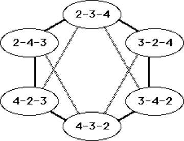
Figure 8. Codimension one connections between regions.

Consider a hexagon $H$ in the common boundary between two regions of $\mathfrak{Geo}^{(6)}.$ Since $H$ can be perturbed slightly to make generic hexagons of either type, $H$ must be of a topological knot type common to both regions. However, the only knot type common to adjacent regions in Figure 8 is the unknot. Therefore hexagons in these codimension one subsets must be unknotted and, in particular, the topological unknots form a single component of geometric unknots in $\mathfrak{Geo}^{(6)}.$

On the other hand, suppose that $h:[0,1]\rightarrow\mathfrak{Geo}^{(6)}$ is a path from some trefoil of type 2-4-3 to some trefoil of type 3-2-4. Since $\mathfrak{Geo}^{(6)}$ is an open subset of $\mathbb{R}^{18},$ there is a small open 18-ball contained in $\mathfrak{Geo}^{(6)}$ about each point in this path. Thus we can assume that whenever $h$ passes through a boundary of one of the six regions, it does so through a generic point in one of the codimension one subsets above. But then $h$ must pass through either 2-3-4 or 4-3-2; see Figure 8. This is a contradiction since only unknots live in these regions. Thus there is no path connecting the trefoils of type 2-4-3 and those of type 3-2-4. Similarly, there is no path between the type 4-2-3 and 3-4-2 trefoils. This proves that $\mathfrak{Geo}^{(6)}$ consists of five path-components: one consisting of unknots, two of right-handed trefoils, and two of left-handed trefoils.

The geometric knot types in $\mathfrak{Geo}^{(6)}$ are completely characterized by a pair of combinatorial invariants which capture a hexagon’s topological chirality (i.e. right- or left-handedness) and geometric curl (i.e. “upward” or “downward” twisting), and are easily computed from the coordinates of a hexagon’s vertices. To define these invariants, let $H=\langle v_{1},v_{2},v_{3},v_{4},v_{5},v_{6}\rangle$ be an embedded hexagon in $\mathbb{R}^{3},$ and consider the open triangular disc determined by vertices $v_{1},v_{2},$ and $v_{3}.$ This disc inherits an orientation from $H$ via the “right hand rule.” Let $\Delta_{2}$ be the algebraic intersection number of the hexagon and this triangle. Notice that the triangular disc can only be pierced by edges $v_{4}v_{5}$ and $v_{5}v_{6}.$ Furthermore, if both of these edges intersect the disc, they will do so in opposite directions, with their contributions to $\Delta_{2}$ canceling out. Thus $\Delta_{2}$ takes on a value of 0, 1, or $-1.$ Similarly, define $\Delta_{4}$ and $\Delta_{6}$ to be the intersection numbers of H with the triangles $\triangle v_{3}v_{4}v_{5}$ and $\triangle v_{5}v_{6}v_{1},$ respectively. By considering the possible values for the $\Delta_{i}$’s (see Lemma 8 in [3]), we can show that

1. $H$ is a right-handed trefoil if and only if $\Delta_{2}=\Delta_{4}=\Delta_{6}=1,$

2. $H$ is a left-handed trefoil if and only if $\Delta_{2}=\Delta_{4}=\Delta_{6}=-1,$ and

3. $H$ is an unknot if and only if $\Delta_{i}=0$ for some $i\in\{2,4,6\},$

implying that the product

(1) $$\Delta(H)=\Delta_{2}\Delta_{4}\Delta_{6},$$

which we call the chirality of $H$, is an invariant under geometric deformations.

Next, we define the curl of $H$ as

(2) $$\mathfrak{curl}\,H=\text{sign}\bigl{(}(v_{3}-v_{1})\times(v_{5}-v_{1})\cdot(v_{2}-v_{1})\bigr{)}.$$

This gives the sign of the $z$-coordinate of $v_{2}$ when we rotate $H$ so that $v_{1},v_{3},$ and $v_{5}$ are placed on the $xy$-plane in a counterclockwise fashion, and therefore measures in some sense whether a hexagon twists up or down. Consider a path $h:[0,1]\rightarrow\mathfrak{Geo}^{(6)}$ which changes the curl of a hexagonal trefoil from +1 to -1. Then there must be some point on this path for which the vector triple product in (2) is equal to zero. At this point, the vertices $v_{1},v_{2},v_{3},$ and $v_{5}$ are all coplanar. However, we can show such a hexagon must be unknotted, giving us a contradiction. In particular, the product $\Delta^{2}(H)\,\mathfrak{curl}\,H$ is also an invariant under geometric deformations. A simple calculation then shows that every trefoil of type 2-4-3 or 4-2-3 has positive curl, while every one of type 3-2-4 or 3-4-2 has negative curl.

Theorem 2.

Define the joint chirality-curl of a hexagon $H$ as the ordered pair $\mathcal{J}(H)=(\Delta(H),\Delta^{2}(H)\,\mathfrak{curl}\,H).$ Then

(3) $$\mathcal{J}(H)=\begin{cases}(0,0)&\text{iff}\,H\,\text{is an unknot,}\\ (+1,c)&\text{iff}\,H\,\text{is a right-handed trefoil with}\,\mathfrak{curl}\,H=c,\\ (-1,c)&\text{iff}\,H\,\text{is a left-handed trefoil with}\,\mathfrak{curl}\,H=c.\end{cases}$$

Therefore the geometric knot type of a hexagon $H$ is completely determined by the value of its chirality and curl.

Before leaving the world of hexagons behind, let us make one last observation. Recall that the construction of $\mathfrak{Geo}^{(n)}$ depends on a choice of a “first vertex” $v_{1}$ and an orientation. This amounts to choosing a sequential labeling $v_{1},v_{2},\ldots,v_{n}$ for the vertices of each polygon. A different choice of labels will lead to a different point in $\mathfrak{Geo}^{(n)}$ corresponding to the same underlying polygon. Thus the dihedral group $\mathbf{D}_{n}$ of order $2n$ acts on $\mathfrak{Geo}^{(n)}$ by shifting or reversing the order of these labels, and this action preserves topological knot type. Observation of the effects on $\mathfrak{curl}\,H$ by the group action of $\mathbf{D}_{6}$ on $\mathfrak{Geo}^{(6)}$ reveals that same statement does not hold true for geometric knot type. In particular, if the group action is defined by the automorphisms

$$r:\langle v_{1},v_{2},v_{3},v_{4},v_{5},v_{6}\rangle \mapsto\langle v_{1},v_{6},v_{5},v_{4},v_{3},v_{2}\rangle,$$

$$s:\langle v_{1},v_{2},v_{3},v_{4},v_{5},v_{6}\rangle \mapsto\langle v_{2},v_{3},v_{4},v_{5},v_{6},v_{1}\rangle,$$

then

$$\mathfrak{curl}\,rH=\mathfrak{curl}\,sH=-\mathfrak{curl}\,H.$$

This shows that the hexagonal trefoil knot is not reversible: In contrast with trefoils in the topological setting, reversing the orientation on a hexagonal trefoil yields a different geometric knot. Furthermore, shifting the labels over by one vertex also changes the the knot type of a trefoil, so that taking quotients under this action we can see that the spaces $\mathfrak{Geo}^{(6)}/\!\prec\!s\!\succ$ of non-based, oriented hexagons, and $\mathfrak{Geo}^{(6)}/\!\prec\!r,s\!\succ$ of non-based, non-oriented hexagons consist of only three components each.

A similar decomposition can be made for the space $\mathfrak{Geo}^{(7)}$ of heptagons. In this case we consider the relative ordering of the half-planes $\mathcal{P}_{2},\mathcal{P}_{3},\mathcal{P}_{4},$ and $\mathcal{P}_{5}$ bounded by the line through $v_{1}$ and $v_{6}.$ This defines 24 open regions which meet along codimension one subsets where two of the $\mathcal{P}_{i}$’s coincide. These junctions can be schematically described as switches in the indices denoting the regions. For instance, regions 2-4-3-5 and 4-2-3-5 meet along a subset consisting of hexagons with $\mathcal{P}_{2}=\mathcal{P}_{4}.$ We can build a model for these connections by taking a vertex for each of the 24 regions and an edge for each codimension-1 subset joining them. The result is a valence-3 graph which forms the 1-dimensional skeleton of a solid zonotope called a permutahedron, shown in Figure  9. Each vertex of the permutahedron is part of a unique square face corresponding to the order-4 sequence of index switches in which the first two indices and the last two indices are switched in an alternating fashion. In addition, each vertex is part of two distinct hexagonal faces which correspond to the order-6 switch sequences in which either the first or last index is fixed while the other three indices are permuted through all six possible orderings. Therefore the valence-3 permutahedron has six square faces and eight hexagonal faces. Extending the edges shared by any two hexagonal faces shows that this is nothing more than a truncated octahedron, also known in crystallography as a Fedorov cubo-octahedron.  ​​

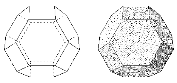
Figure 9. The valence 3 permutahedron.

With a few additional considerations,  ​​ the analysis of the strata over each of these regions shows that $\mathfrak{Geo}^{(7)}$ has a single path-component of unknots and of each topological type of trefoil, and two containing figure-eight knots. Again, these figure-eight knots are new examples of distinct geometric isotopes of the same topological knot, which can be distinguished by a geometric invariant $\Xi,$ defined as follows.

Suppose that $H$ is the heptagon $\langle v_{1},v_{2},v_{3},v_{4},v_{5},v_{6},v_{7}\rangle.$ Define the functions $\Theta_{3}(H)$ and $\Theta_{6}(H)$ as

(4) $$\Theta_{3} =\text{sign}\bigl{(}(v_{7}-v_{1})\times(v_{2}-v_{1})\cdot(v_{3}-v_{1})\bigr{)},$$

$$\Theta_{6} =\text{sign}\bigl{(}(v_{6}-v_{1})\times(v_{7}-v_{1})\cdot(v_{2}-v_{1})\bigr{)}.$$

Then $\Theta_{3}=\Theta_{6}$ if the vertices $v_{3}$ and $v_{6}$ lie on the same side of the plane $\mathcal{P}$ determined by $v_{7},v_{1},$ and $v_{2},$ and $\Theta_{3}=-\Theta_{6}$ if $v_{3}$ and $v_{6}$ lie on different sides of $\mathcal{P}.$ Notice that for a generic heptagon, exactly one of the functions $\frac{1}{2}(\Theta_{3}+\Theta_{6})$ and $\frac{1}{2}(\Theta_{3}-\Theta_{6})$ is zero, while the other is $\pm 1.$

Let $I_{34}$ denote the algebraic intersection number of edge $v_{3}v_{4}$ with the triangular disc $\triangle v_{7}v_{1}v_{2},$ using the usual orientations induced by $H.$ Similarly define $I_{45}$ and $I_{56}$ as the intersection numbers of the triangle $\triangle v_{7}v_{1}v_{2}$ with the edges $v_{4}v_{5}$ and $v_{5}v_{6},$ respectively.

If $H$ has $\Theta_{3}=\Theta_{6},$ then $v_{3}$ and $v_{6}$ lie on the same side of the plane $\mathcal{P}$ so that the three-edge linkage $v_{3}v_{4}v_{5}v_{6}$ will intersect $\mathcal{P}$ at most twice. Furthermore, if both of these intersections happen in the interior of $\triangle v_{7}v_{1}v_{2},$ they occur with opposite orientations. Thus the sum $I_{34}+I_{45}+I_{56}$ only takes on values -1, 0, or 1.

On the other hand, suppose that $H$ is a figure-eight knot with $\Theta_{3}=-\Theta_{6}.$ Then $v_{3}$ and $v_{6}$ lie on the opposite sides of the plane $\mathcal{P}$ so that the three-edge linkage $v_{3}v_{4}v_{5}v_{6}$ intersects $\mathcal{P}$ an odd number of times. First, suppose that there is only one intersection; then the linkage $v_{7}v_{1}v_{2}$ can be piecewise linearly isotoped into a straight line segment. We can think of this isotopy as either pushing $v_{1}$ in a straight line path towards the midpoint of the line segment $v_{2}v_{7},$ or (in the case that the intersection occurs inside $\triangle v_{7}v_{1}v_{2}$) as stretching $v_{7}v_{1}v_{2}$ into a large loop, swinging it like a “jump rope” around and to the other side of the heptagon, and then pushing it in until it coincides with the line segment $v_{2}v_{7}.$ See Figure  10. In either case we get a hexagonal realization of a figure-eight knot. Since this is impossible, the linkage $v_{3}v_{4}v_{5}v_{6}$ has to cross the plane $\mathcal{P}$ three times, and in particular, $v_{3}v_{4}$ and $v_{5}v_{6}$ must do so with the same orientation. Therefore the quantity $I_{34}-I_{56}$ will either be zero (when both edges intersect $\triangle v_{7}v_{1}v_{2},$ or when neither of the two do) or $\pm 1$ (when only one of these intersections occurs inside the triangle).

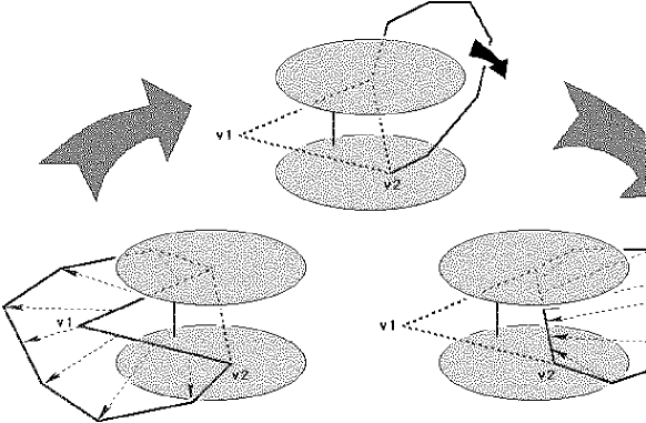
Figure 10. A piecewise linear isotopy of the linkage $v_{7}v_{1}v_{2}.$

A quick look at the possible configurations shows that:

1. if $H$ is a heptagonal figure-eight knot with $\Theta_{3}=\Theta_{6},$ then exactly one of the intersection numbers $I_{34},I_{45},$ or $I_{56}$ is non-zero; thus $I_{34}+I_{45}+I_{56}=\pm 1$ (Lemma 4.2 in [2]), and

2. if $H$ is a heptagonal figure-eight knot with $\Theta_{3}=-\Theta_{6},$ then exactly one of the intersection numbers $I_{34}$ or $I_{56}$ is non-zero; in particular $I_{34}-I_{56}=\pm 1$ (Lemma 4.3 in [2]).

Now consider the function

(5) $$\Xi(H)=\frac{1}{2}\biggl{(}\Theta_{3}+\Theta_{6}\biggr{)}\biggr{(}I_{34}+I_{45}+I_{56}\biggr{)}+\frac{1}{2}\biggl{(}\Theta_{3}-\Theta_{6}\biggr{)}\biggr{(}I_{34}-I_{56}\biggr{)}.$$

By (i) and (ii) above, $\Xi$ can only take values of 1 or -1. Suppose that the value of $\Xi$ changes along some path $h:[0,1]\rightarrow\mathfrak{Geo}^{(7)}.$ Since $\mathfrak{Geo}^{(7)}$ is a manifold, we can assume that, in this path, only one vertex passes through the interior of $\triangle v_{7}v_{1}v_{2}$ at any one time, and that only one edge intersects the line segment $v_{7}v_{2}$ at a time, and that these two things happen at different times. Note that each of these events will change the values of $I_{34}+I_{45}+I_{56}$ and $I_{34}-I_{56}$ by at most one. However, $\Xi$ can only change in increments of two, so if the values of $\Theta_{3}$ and $\Theta_{6}$ remain constant through out $h,$ $\Xi$ must also remain unchanged.

By reversing orientations if necessary, we can assume then that the deformation changes the sign of $\Theta_{3}.$ In particular, let $H_{0}$ be a heptagonal figure-eight knot with $\Theta_{3}=0.$ By pushing $v_{3}$ slightly towards $v_{6},$ we get a heptagon $H_{0}^{+}$ with $\Theta_{3}=\Theta_{6};$ let $I_{34}^{+}$ be the appropriate intersection number for this heptagon. On the other hand, we obtain a heptagon $H_{0}^{-}$ with $\Theta_{3}=-\Theta_{6}$ by pushing $v_{3}$ away from $v_{6};$ let $I_{34}^{-}$ be the corresponding intersection number for this heptagon. By picking $H_{0}^{+}$ and $H_{0}^{-}$ close enough to $H_{0},$ we can assume that the values of the intersection numbers $I_{45}$ and $I_{56}$ coincide for all three knots. This leaves two cases to consider.

First, suppose that $I_{34}^{-}=0.$ Then $I_{56}=\pm 1$ by (ii), and hence $I_{34}^{+}=I_{45}=0$ by (i). Therefore

$$\biggl{(}I_{34}^{+}+I_{45}+I_{56}\biggr{)}=I_{56}=-\biggl{(}I_{34}^{-}-I_{56}\biggr{)}.$$

The extra negative sign in the right hand term of this equation neutralizes the change of sign in $\Theta_{3},$ so that $\Xi$ remains unchanged.

Next, suppose that $I_{34}^{-}=\pm 1,$ in which case $I_{34}^{+}=0.$ Then $I_{56}=0$ by (ii) and $I_{45}=\pm 1$ by (i). Furthermore, the edges $v_{3}v_{4}$ and $v_{4}v_{5}$ must intersect the interior of $\triangle v_{7}v_{1}v_{2}$ from opposite directions, so $I_{34}^{-}=-I_{45}.$ Therefore

$$\biggl{(}I_{34}^{+}+I_{45}+I_{56}\biggr{)}=I_{45}=-I_{34}^{-}=-\biggl{(}I_{34}^{-}-I_{56}\biggr{)},$$

so that, as before, $\Xi$ does not change. This proves the following result.

Theorem 3.

$\Xi$ is an invariant of heptagonal figure-eight knots under geometric deformations.

It is interesting to note that $\Xi$ is also invariant under mirror reflections, since the resulting sign changes in the functions $\Theta_{3},\Theta_{6},I_{34},I_{45},$ and $I_{56}$ cancel out in (5). This reflects the fact that heptagonal figure-eight knots are achiral, i.e. equivalent to their mirror images. Figure  11 shows one such isotopy. Starting with the diagram at the top of Figure  11 and proceeding in a clockwise fashion, we first push $v_{1}$ through the interior of the triangular disc $\triangle v_{2}v_{3}v_{4}.$ Note that in doing so, we may need to change the lengths of one or more of the edges. Although it is difficult to see from the perspective of Figure  11, this motion actually defines an isotopy from the heptagon $\langle v_{1},v_{2},v_{3},v_{4},v_{5},v_{6},v_{7}\rangle$ to the heptagon $\langle-v_{6},-v_{7},-v_{1},-v_{2},-v_{3},-v_{4},-v_{5}\rangle.$ We continue by repeating similar moves, passing $v_{3}$ through $\triangle v_{4}v_{5}v_{6},$ then $v_{5}$ through $\triangle v_{6}v_{7}v_{1},$ and so on. After seven steps, when we move $v_{6}$ past $\triangle v_{7}v_{1}v_{2},$ we arrive at the diagram at the bottom of Figure  11. At this point, the figure-eight knot is the mirror image of the starting position.

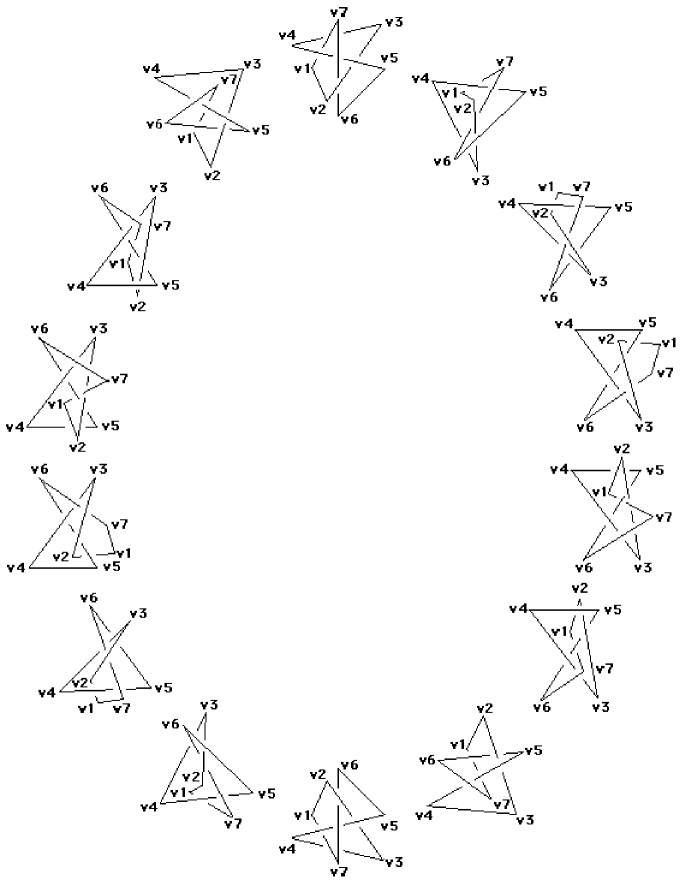
Figure 11. Heptagonal figure-eight knots are achiral.

Finally, consider the $\mathbf{D}_{7}$ action on $\mathfrak{Geo}^{(7)}$ defined by the automorphisms

$$r\langle v_{1},v_{2},v_{3},v_{4},v_{5},v_{6},v_{7}\rangle =\langle v_{1},v_{7},v_{6},v_{5},v_{4},v_{3},v_{2}\rangle$$

$$s\langle v_{1},v_{2},v_{3},v_{4},v_{5},v_{6},v_{7}\rangle =\langle v_{2},v_{3},v_{4},v_{5},v_{6},v_{7},v_{1}\rangle.$$

Reversing the orientation on $H$ via the map $r$ will reverse the orientations on both the edges of $H$ and the triangular discs that they define. In particular,

$$I_{34}(rH)=I_{56}(H)\qquad\qquad I_{45}(rH)=I_{45}(H)\qquad\qquad I_{56}(rH)=I_{34}(H).$$

On the other hand, $r$ not only switches the roles of $\Theta_{3}$ and $\Theta_{6},$ but also changes their signs:

$$\Theta_{3}(rH) =\text{sign}\bigl{(}(v_{2}-v_{1})\times(v_{7}-v_{1})\cdot(v_{6}-v_{1})\bigr{)},$$

$$=-\text{sign}\bigl{(}(v_{6}-v_{1})\times(v_{7}-v_{1})\cdot(v_{2}-v_{1})\bigr{)},$$

$$=-\Theta_{6}(H),$$

$$\Theta_{6}(rH) =\text{sign}\bigl{(}(v_{3}-v_{1})\times(v_{2}-v_{1})\cdot(v_{7}-v_{1})\bigr{)},$$

$$=-\text{sign}\bigl{(}(v_{7}-v_{1})\times(v_{2}-v_{1})\cdot(v_{3}-v_{1})\bigr{)},$$

$$=-\Theta_{3}(H).$$

Therefore

$$\Xi(rH) =\frac{1}{2}\biggl{(}\Theta_{3}(rH)+\Theta_{6}(rH)\biggr{)}\biggr{(}I_{34}(rH)+I_{45}(rH)+I_{56}(rH)\biggr{)}$$

$$\hskip 71.13188pt+\frac{1}{2}\biggl{(}\Theta_{3}(rH)-\Theta_{6}(rH)\biggr{)}\biggr{(}I_{34}(rH)-I_{56}(rH)\biggr{)}$$

$$=\frac{1}{2}\biggl{(}-\Theta_{6}(H)-\Theta_{3}(H)\biggr{)}\biggr{(}I_{56}(H)+I_{45}(H)+I_{34}(H)\biggr{)}$$

$$\hskip 85.35826pt+\frac{1}{2}\biggl{(}-\Theta_{6}(H)+\Theta_{3}(H)\biggr{)}\biggr{(}I_{56}(H)-I_{34}(H)\biggr{)}$$

$$=-\Xi(H).$$

This shows that, like hexagonal trefoil knots, figure-eight knots in $\mathfrak{Geo}^{(7)}$ are irreversible, in contrast with their topological counterparts. However, recall that the irreversibility of trefoils in $\mathfrak{Geo}^{(6)}$ depended strongly on our choice of a “first” vertex $v_{1}.$ In that case, a cyclic permutation of its six vertices would change the trefoil’s geometric knot type. This is not the case for the figure-eight knots in $\mathfrak{Geo}^{(7)},$ for consider the group action induced by the automorphism $s$ on the set of geometric isotopes of the figure-eight knot. This is an order 7 action on a two element set, and must therefore be trivial. In other words, we must have

$$\Xi(sH)=\Xi(H).$$

Hence the distinction in the two figure-eight knot types is an effect of “true” geometric knotting, which goes beyond a simple relabeling of the vertices or our arbitrary choice of first vertex.

3. Knot Projections and Minimal Polygon index

In Section  2, we were concerned with the question of determining, for a given integer $n,$ the number of path-components present in the space $\mathfrak{Geo}^{(n)}$ of $n$-sided polygons. In other words, “how many geometric knot types are there for a particular value of $n$?” However, as $n$ increases, the space $\mathfrak{Geo}^{(n)}$ becomes more and more combinatorially intricate. As this happens, we turn to the question of understanding the number of represented topological (rather than geometric) knot types, and in particular, of how complicated a knot can be realized by an $n$-sided polygon. The answer to this question is only known when $n\leq 8.$ For example, we know there are 9-sided polygonal embeddings of every seven crossing prime knot $(7_{1},\ldots,7_{7})$ as well as the knots $8_{16},8_{17},8_{18},8_{21},9_{40},9_{41},9_{42},$ and $9_{46},$ but presumably this list could be much bigger, and include some of the knots for which we have so far only found 10- or 11-sided realizations. ​​ In this section, we give one of several known bounds on the complexity of an $n$-sided polygon.

Recall that the minimal crossing number of a knot is the smallest number of crossings present in any general position projection of the knot into a plane or sphere. This is the conventional measure of a knot’s complexity, used in the standard notation for knots and links as well as in the knot tables in the appendices of [1], [7], [8], and [16]. We similarly define the minimal polygon index of a knot as the smallest number of edges present in any polygonal embedding of the knot. This invariant, which is elsewhere known as the stick number [1, 5, 6], the broken line number [12], or simply the edge number [9, 15], serves as the corresponding measure of complexity for polygonal knots. These two invariants are traditionally related by the following construction.  ​​

Let $P=\langle v_{1},v_{2},\ldots,v_{n-1},v_{n}\rangle\in\mathfrak{Geo}^{(n)}$ be an $n$-sided polygon embedded in $\mathbb{R}^{3}.$ We project the points in $P$ orthogonally onto a plane perpendicular to one of its edges, say $v_{1}v_{2}.$ This amounts to looking at the polygon from a viewpoint in which we see the edge $v_{1}v_{2}$ “head on,” so that the image of $P$ on our retina (i.e. the plane) is an $(n-1)$-sided polygon. An edge in this image cannot cross either of its two neighbors, or itself, so each edge will intersect at most $n-4$ other edges. Thus for generic polygons in $\mathfrak{Geo}^{(n)},$ this method gives a knot projection with no more than $\tfrac{1}{2}(n-1)(n-4)$ crossings. This leads to the conclusion that if a knot $K$ has minimal crossing number $c(K)$ and minimal polygon index $s(K),$ then

$$c(K)\leq\frac{\bigl{(}s(K)-1\bigr{)}\bigl{(}s(K)-4\bigr{)}}{2},$$

or equivalently (by completing squares and solving for $s$)

$$s(K)\geq\frac{5\,+\,\sqrt{9\,+\,8c(K)}}{2}.$$

For hexagons and heptagons, the bound on crossing number becomes 5 and 9, respectively, well over the actual values of 3 and 4 obtained in Section  2. In fact, the estimated $\tfrac{1}{2}(n-1)(n-4)$ crossings in the image of an $n$-sided polygon can never be achieved when $n$ is odd. Here we present an improvement on the bounds above.

First suppose that we relabel the vertices of $P$ in sequence so that $v_{1}$ is a point on the boundary of the convex hull spanned by the vertices of $P.$ Therefore, we can find a plane $\mathcal{P}_{1}$ which intersects $P$ only at the vertex $v_{1},$ with $P$ lying entirely on one side of $\mathcal{P}_{1}.$

Let $\mathcal{S}$ be a large sphere centered at $v_{1}$ and enclosing all of $P,$ and consider the image of the radial projection $p:P-\{v_{1}\}\rightarrow\mathcal{S}.$ By our choice of $v_{1},$ this image lies entirely in a hemisphere of $\mathcal{S}$ cut by the equator $\mathcal{S}\cap\mathcal{P}_{1}.$ Furthermore, note that the interiors of edges $v_{1}v_{2}$ and $v_{1}v_{n}$ are respectively mapped to the single points $p(v_{2})$ and $p(v_{n}).$ Thus, by picking a generic $P$ in $\mathfrak{Geo}^{(n)},$ we can assume that $\Gamma=p(P-\{v_{1}\})$ consists of a chain of $n-2$ great circular arcs on $\mathcal{S}$ intersecting in four-valent crossings.

Suppose that $\Gamma$ has $c$ crossings. Since $\Gamma$ is contained in a single hemisphere of $\mathcal{S},$ a pair of arcs will intersect at most once. Furthermore adjacent arcs cannot intersect, so each one of the $n-4$ interior arcs $p(v_{3}v_{4}),\ldots,p(v_{n-2}v_{n-1})$ can intersect at most $n-5$ other arcs, while each of the extreme arcs $p(v_{2}v_{3})$ and $p(v_{n-1}v_{n})$ can intersect at most $n-4$ other arcs. Hence

$$c\leq\frac{1}{2}\biggl{(}(n-4)(n-5)+2(n-4)\biggr{)}=\frac{(n-3)(n-4)}{2}.$$

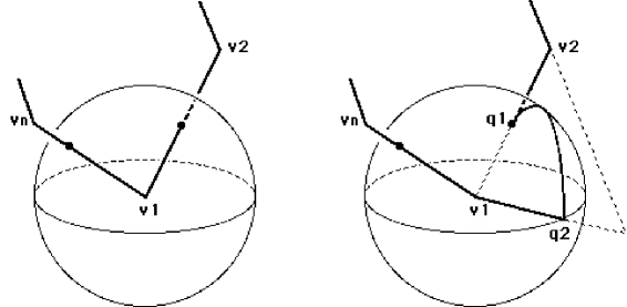
(a)                                                (b)     

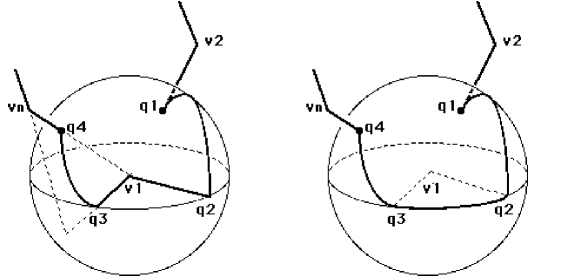
(c)                                                (d)     

Figure 12. Deformation of $P$ inside a small $\epsilon$-ball about $v_{1}.$

Let $\epsilon>0$ be small enough that the closed $\epsilon$-ball $\mathcal{B}_{\epsilon}$ centered at $v_{1}$ intersects the polygon $P$ in exactly two small segments of the edges $v_{1}v_{2}$ and $v_{n}v_{1},$ as shown in Figure  12(a). Suppose that the edge $v_{1}v_{2}$ intersects the sphere $\partial\mathcal{B}_{\epsilon}$ at the point $q_{1}.$ Furthermore, let $q_{2}$ be the point where the equator $\partial\mathcal{B}_{\epsilon}\cap\mathcal{P}_{1}$ intersects the half-plane containing $v_{2}$ and bounded by the line determined by $v_{1}$ and $v_{3}.$ Then we can deform the segment $q_{1}v_{1}$ so that it curves along a great circle path $\alpha_{1}$ from $q_{1}$ to $q_{2},$ and then in a straight line path to $v_{1}.$ See Figure  12(b). Note that since the arc $\alpha_{1}$ lies on the same plane as $v_{2}v_{3},$ then $p(\alpha_{1})\cup p(v_{2}v_{3})$ forms a single great circle trajectory on $\mathcal{S}$ from $p(v_{3})$ to $p(q_{2}).$ Thus, after this deformation, the upper bound on the total number of crossings given above still holds.

Similarly, let $q_{3}$ be the point of intersection between the equator $\partial\mathcal{B}_{\epsilon}\cap\mathcal{P}_{1}$ and the half-plane containing $v_{n}$ and bounded by the line determined by $v_{1}$ and $v_{n-1},$ and let $q_{4}$ be the point at which the edge $v_{n}v_{1}$ intersects $\partial\mathcal{B}_{\epsilon}.$ Then the segment $v_{1}q_{4}$ can be deformed so that it travels in a straight line path from $v_{1}$ to $q_{3}$ and then curves along a great circle path $\alpha_{3}$ from $q_{3}$ to $q_{4}.$ See Figure  12(c). As before, the arc $\alpha_{3}$ lies on the same plane as $v_{n-1}v_{n},$ so $p(v_{n-1}v_{n})\cup p(\alpha_{3})$ forms a single great circle trajectory on $\mathcal{S}$ from $p(v_{n-1})$ to $p(q_{3}).$ Therefore the upper bound on the number of crossings given above still holds after this deformation.

Finally, isotope $P$ by moving $v_{1}$ into the interior of the triangle $\triangle q_{2}v_{1}q_{3}$ while curving the segments $q_{2}v_{1}$ and $v_{1}q_{3}$ until they coincide with an arc along the equator $\partial\mathcal{B}_{\epsilon}\cap\mathcal{P}_{1},$ as in Figure  12(d). This final transformation turns $P$ into a non-polygonal embedding of the same (topological) knot type; this new embedding agrees with $P$ outside of the ball $\mathcal{B}_{\epsilon}$ but completely avoids its interior. In the meanwhile, the image under $p$ of this embedding is simply a (spherical) knot projection $\Gamma^{\prime}$ consisting of the $n-2$ arcs of $\Gamma$ (with its ends extended by $p(\alpha_{1})$ and $p(\alpha_{3})$), together with an $(n-1)$th arc $\alpha_{2}$ running along the equator $\mathcal{S}\cap\mathcal{P}_{1}$ and joining the endpoints $p(q_{2})$ and $p(q_{3}).$ Since $\Gamma$ is contained entirely on one side of the equator, $\alpha_{2}$ does not cross any other arcs. Hence the new projection has no more crossings than it did before the last deformation, proving the following theorem.

Theorem 4.

Suppose that a knot $K$ with minimal crossing number $c(K)$ and minimal polygon index $s(K).$ Then

(6) $$c(K)\leq\frac{\bigl{(}s(K)-3\bigr{)}\bigl{(}s(K)-4\bigr{)}}{2}.$$

Completing the square in (6) shows that

$$2c\leq s^{2}-\,7s\,+\,12=\biggl{(}s-\frac{7}{2}\biggr{)}^{2}-\frac{1}{4},$$

so that

$$s(K)\geq\frac{7\,+\,\sqrt{8c(K)\,+\,1}}{2}.$$

Note that Theorem  4 correctly predicts that the trefoil is the only non-trivial knot which can be realized with six edges.

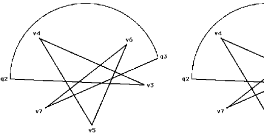
(a)                                                           (b)

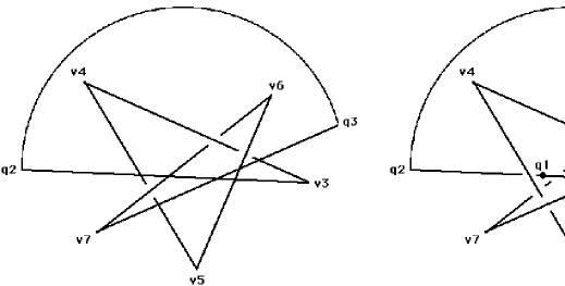
(c)                                                           (d)

Figure 13. A knot universe and several choices in over- and under-crossings.

In the case of octagons, the new bound on crossing number becomes 10. However, in [2] we systematically look at the possible knot projections $\Gamma^{\prime}$ resulting from the deformation described by Figure  12 and thereby enumerate the topological knots which are appear in $\mathfrak{Geo}^{(8)}.$ For example, consider the ten-crossing knot universe shown in Figure  13(a). By appropriately choosing at each crossing which strand goes “over” and which one goes “under,” we will obtain a knot projection $\Gamma^{\prime}$ corresponding, as above, to some octagon $P.$ As we make choices in “over” and “under” crossings we need to keep a few points in mind:

1. If $v_{2}v_{3}$ passes under every one of its crossings, then the interior of the triangular disc $\triangle v_{1}v_{2}v_{3}$ does not intersect the rest of $P.$ In this case, $P$ can be isotoped by pushing $v_{2}$ in a straight line path to the midpoint of the line segment $v_{1}v_{3}$ until $P$ coincides with a heptagon. A similar isotopy exists if $v_{7}v_{8}$ contributes only “under” crossings. Therefore we need not consider these diagrams.

2. If the edges $v_{5}v_{6}$ and $v_{6}v_{7}$ both go under $v_{3}v_{4},$ as in Figure  13(b), then we can isotope $P$ so that the corresponding $\Gamma^{\prime}$ has two fewer crossings. For instance, we can shrink the lengths of $v_{5}v_{6}$ and $v_{6}v_{7},$ in essence performing a Reidemeister 2 move. We can therefore ignore crossing choices which permit a reducing isotopy of this type, delaying their analysis until we examine the resulting reduced diagram.

3. Some choices of “over” and “under” crossings will lead to configurations which are impossible to create with straight edges. For instance, consider the three crossing choices made in Figure  13(c). Let $\mathcal{P}$ be the plane containing $v_{4},v_{5},$ and $v_{6}.$ Note that the interior of edge $v_{6}v_{7}$ lies entirely above the plane $\mathcal{P},$ since it starts on the plane at $v_{6}$ and then crosses over $v_{4}v_{5}.$ Similarly, the interior of edge $v_{3}v_{4}$ lies below the plane $\mathcal{P}$ since it crosses under $v_{5}v_{6}$ and then meets the plane at $v_{4}.$ This means that $v_{3}v_{4}$ cannot cross over $v_{6}v_{7},$ as in Figure  13(c), unless one of the two edges is bent.

4. A particularly tricky example of a bad “over” and “under” crossing choice is shown in Figure  13(d). This diagram corresponds to an octagonal realization of the knot $8_{18},$ shown in Figure  14. Here the problem is not as obvious as before. In fact, among all of the projections corresponding to impossible configurations which we encounter in [2], this is the only one which is not clearly impossible. Nonetheless, through a delicate balance between introducing self-intersections and counting dimensions, we can show that there is no way to construct this configuration. The details of this argument will appear in a forthcoming paper.

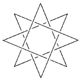
Figure 14. This octagonal embedding of the knot $8_{18}$ cannot be constructed with straight edges.

After considering all possible projections $\Gamma^{\prime}$ with more than six crossings, we find that the only knots with polygon index 8 and crossing number greater than 6 are $8_{19}$ and $8_{20}.$ Since it is known that there are octagonal realizations of every knot $K$ with crossing number $c(K)\leq 6,$ we obtain a complete list of the topological knots present in $\mathfrak{Geo}^{(8)},$ as indicated in Theorem  1(iv). With the exception of $6_{3},$ the square knot $3_{1}-3_{1},$ the figure-eight knot $4_{1},$ and the unknot, every knot type in this list is chiral and therefore must contribute at least two path-components in $\mathfrak{Geo}^{(8)}.$ Therefore $\mathfrak{Geo}^{(8)}$ will contain at least twenty path-components.

References

- [1] C. C. Adams, The knot book: An elementary introduction to the mathematical theory of knots, W. H. Freeman and Co., New York, 1994.
- [2] J. A. Calvo, Geometric knot theory: the classification of spatial polygons with a small number of edges, Ph.D. thesis, University of California, Santa Barbara, 1998.
- [3] by same author, The embedding space of hexagonal knots, preprint, 1999.
- [4] J. A. Calvo and K. C. Millett, Minimal edge piecewise linear knots, Ideal Knots (A. Stasiak, V. Katrich, and L. H. Kauffman, eds.), Series on Knots and Everything, vol. 19, World Scientific, Singapore, 1999, pp. 107 – 128.
- [5] C. C. Adams, B. M. Brennan, D. L. Greilsheimer, and A. K. Woo, Stick numbers and composition of knots and links, Journal of Knot Theory and its Ramifications 6 (1997), no. 2, 149–161.
- [6] E. Furstenberg, J. Lie, and J. Schneider, Stick knots, preprint, 1997.
- [7] L. H. Kauffman, On knots, Annals of Mathematics Studies, vol. 115, Princeton University Press, Princeton, NJ, 1987.
- [8] C. Livingston, Knot theory, Carus Mathematical Monographs, vol. 24, Mathematical Association of America, Washington, DC, 1993.
- [9] M. Meissen, Edge number results for piecewise-linear knots, Knot Theory, Polish Academy of Sciences, Warsaw, 1998, pp. 235–242.
- [10] K. C. Millett, Knotting of regular polygons in 3-space, Journal of Knot Theory and its Ramifications 3 (1994), no. 3, 263–278; also in [11] pp. 31–46.
- [11] K. C. Millett and D. W. Sumners (eds.), Random knotting and linking, Series on Knots and Everything, vol. 7, World Scientific, Singapore, 1994.
- [12] S. Negami, Ramsey theorems for knots, links, and spatial graphs, Transactions of the American Mathematical Society 324 (1991), no. 2, 527–541.
- [13] R. Randell, A molecular conformation space, MATH/CHEM/COMP 1987 (R. C. Lacher, ed.), Studies in Physical and Theoretical Chemistry, vol. 54, Elsevier Science, Amsterdam, 1988, pp. 125 –140.
- [14] by same author, Conformation spaces of molecular rings, MATH/CHEM/COMP 1987 (R. C. Lacher, ed.), Studies in Physical and Theoretical Chemistry, vol. 54, Elsevier Science, Amsterdam, 1988, pp. 141 –156.
- [15] by same author, An elementary invariant of knots, Journal of Knot Theory and its Ramifications 3 (1994), no. 3, 279–286; also in [11] pp. 47–54.
- [16] D. Rolfsen, Knots and links, Mathematical Lecture Series, vol. 7, Publish or Perish, Houston, TX, 1976.
- [17] A. E. H. Tutton, Crystallography and practical crystal measurement, vol. 1, Macmillan and Co. Ltd., London, 1922.
- [18] H. Whitney, Elementary structure of real algebraic varieties, Annals of Mathematics 66 (1967), 545 –556.
- [19] G. M. Ziegler, Lectures on polytopes, Graduate Texts in Mathematics, vol. 152, Springer Verlag, New York, 1995.