Castelnuovo function, zero-dimensional schemes and singular plane curves

Abstract.

We study families $V$ of curves in ${\mathbb{P}}^{2}({\mathbb{C}})$ of degree $d$ having exactly $r$ singular points of given topological or analytic types. We derive new sufficient conditions for $V$ to be T-smooth (smooth of the expected dimension), respectively to be irreducible. For T-smoothness these conditions involve new invariants of curve singularities and are conjectured to be asymptotically proper, i.e., optimal up to a constant factor. To obtain the results, we study the Castelnuovo function, prove the irreducibility of the Hilbert scheme of zero-dimensional schemes associated to a cluster of infinitely near points of the singularities and deduce new vanishing theorems for ideal sheaves of zero-dimensional schemes in ${\mathbb{P}}^{2}$. Moreover, we give a series of examples of cuspidal curves where the family $V$ is reducible, but where $\pi_{1}({\mathbb{P}}^{2}\!\setminus\!\!\>C)$ coincides (and is abelian) for all $C\in V$.

Introduction

Statement of the problem and asymptotically proper bounds

Singular algebraic curves, their existence, deformation, families (from the local and global point of view) attract continuous attention of algebraic geometers since the last century. The geometry of equisingular families of algebraic curves on smooth algebraic surfaces has been founded in basic works of Plücker, Severi, Segre, Zariski, and has tight links and finds important applications in singularity theory, topology of complex algebraic curves and surfaces, and in real algebraic geometry.

In the present paper we consider the family $V_{d}^{\text{\it irr}}(S_{1},\dots,S_{r})$ of reduced irreducible complex plane curves of degree $d$ with $r$ isolated singular points of given topological, or analytic types $S_{1},\dots,S_{r}$ (further referred to as equisingular families, or ESF). The questions about the non-emptiness, smoothness, irreducibility and dimension are basic in the geometry of ESF. Except for the case of nodal curves, no complete answers are known and one can hardly expect them.

Our goal, however, is to obtain asymptotically proper sufficient conditions for ESF to have “good” properties like being non-empty, or smooth, or irreducible. The conditions should be expressed in the form of bounds to numerical invariants of curves and singularities such that, for the “good” properties to hold, the necessary respectively sufficient conditions should be given by inequalities with the same invariants but, maybe, with different absolute constants. As an example, we mention our sufficient condition for the non-emptiness of $V_{d}^{\text{\it irr}}(S_{1},\dots,S_{r})$ with topological singularities $S_{1},\dots,S_{r}$ [GLS1, Lo, Lo1]

$$\textstyle{\sum\limits_{i=1}^{r}}\mu(S_{i})<\tfrac{1}{46}\cdot(d+2)^{2}\ ,$$ (0.1)

whereas the classically known necessary condition is

$$\textstyle{\sum\limits_{i=1}^{r}}\mu(S_{i})\leq(d-1)^{2}\ .$$ (0.2)

In the present paper we obtain two qualitatively new bounds: one for the smoothness of $V_{d}^{\text{\it irr}}(S_{1},\dots,S_{r})$ and one for the irreducibility. In particular, we show that the inequality

$$\textstyle{\sum\limits_{i=1}^{r}}\gamma(S_{i})<d^{2}+6d+8\,,$$ (0.3)

where $\gamma(S)$ is a new singularity invariant (defined in Section 2.1), is sufficient for the smoothness and expected dimension (also called T-property) of $V_{d}^{\text{\it irr}}(S_{1},\dots,S_{r})$. We expect (0.3) to be asymptotically proper for topological singularities in the following sense:

Conjecture 0.1.

There exists an absolute constant $A>0$ such that for any topological singularity $S$ there are infinitely many pairs $(r,d)\in{\mathbb{N}}\!\>^{2}$ such that $V_{d}^{\text{\it irr}}(r\!\!\>\cdot\!\!\>S)$ is empty or not smooth or has dimension greater than the expected one and

$$r\cdot\gamma(S)\>\leq\>A\cdot d^{2}.$$

We know that the exponent $2$ of $d$ in the right-hand side of (0.3) cannot be raised in any reasonable sufficient criterion for T-property with the left-hand side being the sum of local singularity invariants. Hence, for an asymptotically proper sufficient criterion for T-property the right-hand side is correct. On the other hand, for the left-hand side of such a sufficient criterion different invariants can be used. What we conjecture is that the new invariant $\gamma(S)$ is the “correct” one for an asymptotically proper bound in the case of topological singularities.

The conjecture is known to be true for an infinite series of singularities of types $A$ and $D$ (cf. [Sh5, GLS2]) and it holds for ordinary singularities, because here the inequality (0.3) is implied by

$$4\cdot\#(\text{nodes\/})+18\cdot\#(\text{triple points\/})+\textstyle{\sum\limits_{\operatorname{mt}S_{i}>3}}\tfrac{16}{7}\cdot(\operatorname{mt}S_{i})^{2}\><\>d^{2}+6d+8\,,$$ (0.4)

(cf. Corollary 2.5) whereas the inequality

$$\textstyle{\sum\limits_{i=1}^{r}}\operatorname{mt}S_{i}(\operatorname{mt}S_{i}-1)\>\leq\>(d-1)(d-2)$$

is necessary for the existence of an irreducible curve with ordinary singularities $S_{1},\dots,S_{r}$.

New criteria for smoothness and irreducibility of equisingular families

We show that under condition (0.3) (with singularity invariants $\gamma(S)\leq(\tau^{\prime}(S)\!\!\;+\!\!\;1)^{2}$, where $\tau^{\prime}$ stands for the Tjurina number $\tau$ if $S$ is an analytic type and for $\tau^{\text{es}}=\mu-\text{modality}$ if $S$ is a topological type) the family $V=V_{d}^{\text{\it irr}}(S_{1},\dots,S_{r})$ is either empty or smooth of the expected dimension (Theorem 1 in Section 2). In addition, for any curve $C\in V_{d}^{\text{\it irr}}(S_{1},\dots,S_{r})$ the inequality (0.3) with analytic invariants $\gamma$ is sufficient for the independence of versal deformations of all singular points when varying in the space of plane curves of degree $d$.

This improves the previously known condition (cf. [GLS2])

$$\textstyle{\sum\limits_{i=1}^{r}}(\tau^{\prime}(S_{i})+1)^{2}\><\>d^{2}\,,$$

mainly with respect to the singularity invariants in the left-hand side. For instance, for an ordinary singular point $S$ of multiplicity $m$, considered up to topological equivalence,

$$(\tau^{\prime}(S)+1)^{2}=\bigl{(}\tfrac{m(m+1)}{2}-1\bigr{)}^{2}\ \sim\ \tfrac{1}{4}m^{4},$$

whereas the invariant in the left-hand side of the new condition is $\gamma(S)\leq\frac{16}{7}\!\;m^{2}$ (cf. (0.4)).

Another new result concerns the irreducibility of ESF. It says that under the conditions $\max_{i}\tau^{\prime}(S_{i})\leq\frac{2}{5}\!\;d-1$ and

$$\tfrac{25}{2}\cdot\#(\text{nodes})+18\cdot\#(\text{cusps})+\tfrac{10}{9}\cdot\!\textstyle{\sum\limits_{\tau^{\prime}(S_{i})\geq 3}}(\tau^{\prime}(S_{i})\!+\!2)^{2}\,<\>d^{2}$$ (0.5)

the family $V_{d}^{\text{\it irr}}(S_{1},\dots,S_{r})$ is irreducible (cf. Theorem 2 in Section 3 with a slightly stronger statement). The irreducibility criterion (0.5) improves the bounds known before

$$\textstyle{\sum\limits_{i=1}^{r}}\mu(S_{i})\,<\,\min\limits_{1\leq i\leq r}f(S_{i})\cdot d^{2},$$ (0.6)

$$f(S)\,=\,\tfrac{2}{(\mu(S)+\operatorname{mt}S-1)^{2}(3\mu(S)-(\operatorname{mt}S)^{2}+3\cdot\operatorname{mt}S+2)^{2}}\,,$$

obtained in [Sh4], and

$$\textstyle{\sum\limits_{i=1}^{r}}\alpha(S_{i})\,<\,\tfrac{2\alpha-3}{2\alpha(\alpha-1)}\cdot d^{2}-\tfrac{2\alpha-9}{2(\alpha-1)}\cdot d-\tfrac{4\alpha}{\alpha-1}\,,\quad\alpha\,:=\,\max\limits_{1\leq i\leq r}\alpha(S_{i})\,,$$ (0.7)

where $\alpha(\text{node})=3$, $\alpha(\text{cusp})=5$ and $\alpha(S)\geq\frac{10}{9}(\tau^{\prime}(S)+2)$ for other singularities $S$, obtained in the Appendix to [Ba]. We like to point out that the coefficient of $d^{2}$ in (0.6) and in (0.7) depends on the “worst” singularity, hence these sufficient conditions are weakened significantly when adding one complicated singularity. On the other hand, the new condition (0.5) contains the contributions of the singularities in an additive form, whence it is not so sensitive to adding an extra singularity.

Curves with nodes and cusps

We pay a special attention to the classical case of families of curves with $n$ nodes and $k$ cusps, for which the criteria (0.3), (0.5) appear to be

$$4n+9k\,<\,d^{2}+6d+8\,,\quad\mbox{respectively}\quad\tfrac{25}{2}\!\>n+18k\,<\,d^{2}\,,$$ (0.8)

(Corollaries 2.4, 3.2). This is stronger than the previously known sufficient conditions for the smoothness of $V_{d}^{\text{\it irr}}(n\!\!\;\cdot\!\!\>A_{1},\ k\!\!\;\cdot\!\!\>A_{2})$,

$$4n+9k<d^{2}\quad\mbox{(cf.\ \cite[cite]{[\@@bibref{}{GLS97}{}{}]})}\,,$$

and for the irreducibility,

$$225\!\>n+450\!\>k\,<\,d^{2}\quad\text{(cf.\ \cite[cite]{[\@@bibref{}{Shu94}{}{}]})}\quad\text{and}\quad\tfrac{120}{7}\!\>n+\tfrac{200}{7}\!\>k\,<\,d^{2}-\tfrac{5}{7}\!\>d-\tfrac{200}{7}\quad\text{(cf.\ \cite[cite]{[\@@bibref{}{Barkats}{}{}]})}\,.$$

We note also that for families of cuspidal curves our smoothness criterion is quite close to an optimal one: the above inequalities provide the smoothness and expected dimension of $V_{d}^{\text{\it irr}}(k\!\!\;\cdot\!\!\>A_{2})$ for $k\leq\frac{1}{9}d^{2}\!\!\>+O(d)$, whereas the families of irreducible curves of degree $d$ with $k=\frac{6}{49}d^{2}\!\!\>+O(d)$ cusps, constructed in [Sh3], are either nonsmooth, or have dimension greater than the expected one. That is, the coefficient $\frac{1}{9}$ of $d^{2}$ differs from an optimal one by a factor $\leq 1.1$.

Concerning the irreducibility it was proven in [Sh3] that the variety $V=V_{d}^{\text{\it irr}}(6p^{2}\!\cdot\!\!\>A_{2})$ of cuspidal curves of degree $d$ with precisely $6p^{2}$ cusps has at least two components for $d=6p$, showing that the coefficient $\frac{1}{18}$ of $d^{2}$ in (0.5) differs from an optimal one by a factor $\leq 3$. These examples generalize the classical example of sextic curves having 6 cusps given by Zariski [Za]. In Proposition 3.4 we modify the construction to obtain curves of degree $d$ slightly bigger than $6p$ having $6p^{2}$ cusps such that the corresponding ESF $V$ has at least two irreducible components but, different to Zariski’s example, $\pi_{1}({\mathbb{P}}^{2}\!\setminus\!\!\>C)={\mathbb{Z}}/d{\mathbb{Z}}$ for each $C\in V$. We do not know whether $V$ is connected.

Principal approach

Looking for a sufficient smoothness and irreducibility condition, applicable to families of curves with arbitrary singularities, we use the fact that the smoothness and expected dimension of an equisingular family $V$ follow from the $h^{1}$-vanishing for the ideal sheaves of some zero-dimensional subschemes of the plane (or another smooth surface) associated with any curve $C\in V$ (see [GK, GL] for a detailed general setting), and that the irreducibility of $V$ follows from the $h^{1}$-vanishing for the ideal sheaf of certain zero-dimensional schemes associated with a generic curve $C\in V$ (such an approach was realized, for instance, in [Sh3, Sh4, Ba]).

Various $h^{1}$-vanishing criteria have been used in connection with the problems stated. The classical idea, applied by Severi [Se], Segre, Zariski [Za] through the later development [GK, Sh1], is to restrict the ideal sheaf to the curve $C\in V$ itself. For many cases one obtains better results when replacing $C$ by a polar curve [Sh, GL], or a special auxiliary curve [Sh3, Sh4]. A similar idea combined with Horace’s method can be found in [Sh5, GLS]. Chiantini and Sernesi [CS] applied Bogomolov’s theory of unstable rank two vector bundles on surfaces for the smoothness problem of families of nodal curves, which then was extended to curves with arbitrary singularities [GLS2]. It was Barkats [Ba] who showed how to apply the Castelnuovo function and Davis’ Theorem [Da] for the computation of $h^{1}$ in relation to the irreducibility problem.

In the present paper we strongly exploit Barkats’ observation, combining it with other tools. Moreover, we perform our computations in a different way to obtain stronger $h^{1}$-vanishing theorems (cf. Proposition 2.1 and Lemma 5.3). Finally, we derive sufficient irreducibility conditions with better asymptotic behavior (see explanation above), which involve both, topological and analytic, singularities. A similar approach is used for the smoothness problem completing with the result (0.3).

Further results and distribution of the material

For the convenience of the reader we present the material in a self-contained form. In Section 1 we introduce and set up the theory of zero-dimensional schemes associated to singular points. In Sections 1.2 (respectively 1.4) we do this for topological (respectively analytic) singularities. Section 1.3 contains a proof for the existence and irreducibility of the Hilbert scheme associated to generalized singularity schemes, or, for clusters (answering a question of Kleiman and Piene).

We compute several invariants of plane curve singularities, for instance, we determine the degree of $C^{0}$-sufficiency (correcting the result in [Li]), cf. Lemmas 1.4 and 1.5. In Section 1.5 we recall basic facts about the Castelnuovo function of a zero-dimensional scheme in ${\mathbb{P}}^{2}$.

In Sections 2 and 3 we formulate the main results on the smoothness and irreducibility of equisingular families of curves, in particular, we introduce the new invariants $\gamma(C;X)$ (cf. Section 2.1). Sections 4 and 5 contain the proofs of the main results.

Basic definitions and notations

Two germs $(C,z)\subset({\mathbb{P}}^{2}\!,z)$ and $(D,w)\subset({\mathbb{P}}^{2}\!,w)$ of reduced plane curve singularities (or any of their defining power series) are said to be topologically equivalent (respectively analytically equivalent, also called contact equivalent) if there exists a local homeomorphism (respectively analytic isomorphism) $({\mathbb{P}}^{2}\!,z)\to({\mathbb{P}}^{2}\!,w)$ mapping $(C,z)$ to $(D,w)$. The corresponding equivalence classes are called topological (resp. analytic) types.

We recall the notion of families of plane curves that will be used in the following. Let $T$ be a complex space, then by a family of (reduced, irreducible) plane curves over $T$ we mean a commutative diagram

$$\begin{array}[]{lcl}\;{\mathcal{C}}&\stackrel{{\scriptstyle j}}{{\hookrightarrow}}&\;\;{\mathbb{P}}^{2}\!\times T\\ \scriptstyle{\varphi}\textstyle{\searrow}&&\swarrow\scriptstyle{pr}\\ &T&\end{array}$$

where $\varphi$ is a proper and flat morphism such that for all points $t\in T$ the fibre ${\mathcal{C}}_{t}:=\varphi^{-1}(t)$ is a (reduced, irreducible) plane curve, $j:{\mathcal{C}}\hookrightarrow{\mathbb{P}}^{2}\!\times T$ is a closed embedding and $pr$ denotes the natural projection. In a similar manner, one defines (flat) families of zero-dimensional schemes in ${\mathbb{P}}^{2}$ (respectively in a surface $\Sigma$).

A family with sections is a diagram as above, together with sections $\sigma_{1},\dots,\sigma_{r}:T\to{\mathcal{C}}$ of $\varphi$. The sections are called trivial if $\sigma_{i}$ is an isomorphism $T\to\{z_{i}\}\times T$ for some $z_{i}\in{\mathbb{P}}^{2}$.

To a family of reduced plane curves as above and a fibre $C={\mathcal{C}}_{t_{0}}$ we can associate, in a functorial way, the deformation $\coprod_{i}({\mathcal{C}},z_{i})\to(T,t_{0})$ of the multigerm $(C,\text{Sing}\,C)=\coprod_{i}(C,z_{i})$ over the germ $(T,t_{0})$. Having a family with sections $\sigma_{1},\dots,\sigma_{r}$, $\sigma_{i}(t_{0})=z_{i}$, we obtain in the same way a deformation of $\coprod_{i}(C,z_{i})$ over $(T,t_{0})$ with sections.

A family ${\mathcal{C}}\hookrightarrow{\mathbb{P}}^{2}\!\times T\to T$ of reduced curves (with sections) is called equianalytic, respectively equisingular (along the sections) if, for each $t\in T$, the induced deformation of the multigerm $({\mathcal{C}}_{t},\text{Sing}\,{\mathcal{C}}_{t})$ is isomorphic (isomorphic as deformation with section) to the trivial deformation, respectively to an equisingular deformation along the trivial section (for the equisingular case cf. [Wa]).

The Hilbert scheme of plane curves of degree $d$ together with its universal family is the family of all curves of degree $d$ in ${\mathbb{P}}^{2}$, the base space may be identified with the linear system $\big{|}H^{0}\bigl{(}{\mathcal{O}}_{{\mathbb{P}}^{2}}(d)\bigr{)}\big{|}$. We are interested in subfamilies of curves in ${\mathbb{P}}^{2}$ having fixed analytic, respectively topological types of their singularities.

To be specific, let $S_{1},\dots,S_{r}$ be fixed analytic, respectively topological types. Denote by $V_{d}(S_{1},\dots,S_{r})$ the space of reduced curves $C\subset{\mathbb{P}}^{2}$ of degree $d$ having precisely $r$ singularities which are of types $S_{1},\dots,S_{r}$. By [GL], Proposition 2.1, $V_{d}(S_{1},\dots,S_{r})$ is a locally closed subscheme of $\big{|}H^{0}\bigl{(}{\mathcal{O}}_{{\mathbb{P}}^{2}}(d)\bigr{)}\big{|}$ and represents the functor of equianalytic, respectively equisingular families of given types $S_{1},\dots,S_{r}$.

In the following, by abuse of notation, we write $C\in V_{d}(S_{1},\dots,S_{r})$ to denote either the point in $V_{d}(S_{1},\dots,S_{r})$ or the curve corresponding to the point, that is, the corresponding fibre in the universal family.

Acknowledgements

We should like to thank Ragni Piene for helpful remarks concerning the Hilbert scheme studied in Section 1.3 and for the reference to the paper [NV].

1. Zero-dimensional schemes

1.1. Geometrical meaning of zero-dimensional schemes and $h^{1}$-vanishing

Throughout the paper, we work with zero-dimensional schemes $X=X(C)$ that are contained in a reduced plane curve $C\subset{\mathbb{P}}^{2}$ and concentrated in finitely many points $z$. The corresponding ideal sheaves will be denoted by ${\mathcal{J}}_{X/{\mathbb{P}}^{2}}\subset{\mathcal{O}}_{{\mathbb{P}}^{2}}$. Moreover, we denote

$$\deg X:=\textstyle{\sum\limits_{z}}\dim_{\mathbb{C}}{\mathcal{O}}_{{\mathbb{P}}^{2},z}/({\mathcal{J}}_{X/{\mathbb{P}}^{2}})_{z}\,,\qquad\operatorname{mt}(X,z):=\max\left\{\nu\in{\mathbb{Z}}\,\big{|}\,({\mathcal{J}}_{X/{\mathbb{P}}^{2}})_{z}\subset\mathfrak{m}_{z}^{\nu}\right\}\,,$$

with ${\mathcal{O}}_{{\mathbb{P}}^{2},z}$ the analytic local ring at $z$ and $\mathfrak{m}_{z}\subset{\mathcal{O}}_{{\mathbb{P}}^{2},z}$ the maximal ideal.

Let $C$ be a reduced plane curve and let $\text{Sing}\,C=\{z_{1},\dots,z_{r}\}$ be its singular locus. We shall consider, among others, the following schemes $X$:

1. $X^{\text{ea}}(C)=X^{\text{ea}}(C,z_{1})\cup\ldots\cup X^{\text{ea}}(C,z_{r})$, the zero-dimensional scheme concentrated in $\text{Sing}\,C$ defined by the Tjurina ideals

   $$I^{\text{ea}}(C,z_{i})\,:=\,j(C,z_{i})\,=\,\langle\,f,\tfrac{\partial f}{\partial x},\tfrac{\partial f}{\partial y}\,\rangle\,\subset\,{\mathcal{O}}_{{\mathbb{P}}^{2},z_{i}}\,,$$

   (where $f(x,y)=0$ is a local equation for $(C,z_{i})$). $I^{\text{ea}}(C,z_{i})$ is the tangent space to equianalytic, i.e., analytically trivial deformations of $(C,z_{i})$.

2. $X^{\text{es}}(C)=X^{\text{es}}(C,z_{1})\cup\ldots\cup X^{\text{es}}(C,z_{r})$, the zero-dimensional scheme defined by the equisingularity ideals

   $$I^{\text{es}}(C,z_{i})\,:=\,\bigl{\{}\,g\in{\mathcal{O}}_{{\mathbb{P}}^{2},z_{i}}\>\big{|}\>f+\varepsilon g\text{ is equisingular over Spec}\,({\mathbb{C}}[\varepsilon]/\varepsilon^{2})\,\bigr{\}}\,.$$

   Note that $X^{\text{es}}(C)$ is contained in $X^{\text{ea}}(C)$ (cf. [Wa]). $I^{\text{es}}(C,z_{i})$ is the tangent space to equisingular deformations of $(C,z_{i})$.

3. $X^{\text{ea}}_{\text{fix}}(C)=X^{\text{ea}}_{\text{fix}}(C,z_{1})\cup\ldots\cup X^{\text{ea}}_{\text{fix}}(C,z_{r})$ the zero-dimensional scheme defined by the ideals

   $$I^{\text{ea}}_{\text{fix}}(C,z_{i})\,:=\,\langle f\rangle+\mathfrak{m}_{z_{i}}\!\!\!\>\cdot\!\!\>j(C,z_{i})\,\subset\,j(C,z_{i})\,,$$

   where $\mathfrak{m}_{z_{i}}=\mathfrak{m}_{{\mathbb{P}}^{2},z_{i}}\subset{\mathcal{O}}_{{\mathbb{P}}^{2},z_{i}}$ denotes the maximal ideal. $I^{\text{ea}}_{\text{fix}}(C,z_{i})$ is the tangent space to equianalytic deformations of $(C,z_{i})$ with fixed position of the singularity, i.e., equianalytic deformations along the trivial section.

4. $X^{\text{es}}_{\text{fix}}(C)=X^{\text{es}}_{\text{fix}}(C,z_{1})\cup\ldots\cup X^{\text{es}}_{\text{fix}}(C,z_{r})$ the zero-dimensional scheme defined by the ideals

   $$I^{\text{es}}_{\text{fix}}(C,z_{i})\,:=\,\Bigl{\{}g\in{\mathcal{O}}_{{\mathbb{P}}^{2},z_{i}}\>\Big{|}\>\begin{array}[]{c}\scriptstyle{f+\varepsilon g\text{ is equisingular over Spec}\,({\mathbb{C}}[\varepsilon]/\varepsilon^{2})}\\ \text{\scriptsize along the trivial section}\end{array}\Bigr{\}}\subset I^{\text{es}}(C,z_{i})\,.$$

   $I^{\text{es}}_{\text{fix}}(C,z_{i})$ is the tangent space to equisingular deformations of $(C,z_{i})$ with fixed position of the singularity.

5. $X^{s}(C)=X^{s}(C,z_{1})\cup\ldots\cup X^{s}(C,z_{r})$ the zero-dimensional scheme introduced in [GLS1] in order to handle the topological types of the singularities (cf. Section 1.2).

6. $X^{a}(C)=X^{a}(C,z_{1})\cup\ldots\cup X^{a}(C,z_{r})$ the zero-dimensional scheme introduced in this paper in order to handle the analytic types of the singularities (cf. Section 1.4). In order to apply these schemes, we shall have, however, to consider also (slightly) bigger schemes $\widetilde{X}^{a}(C)\supset X^{a}(C)$.

The importance of the schemes $X(C)$ comes from the fact that the cohomology groups $H^{i}\bigl{(}{\mathcal{J}}_{X(C)/{\mathbb{P}}^{2}}(d)\bigr{)}$ have a precise geometric meaning for the space $V_{d}(S_{1},\dots,S_{r})$. To explain this for $X^{\text{ea}}_{\text{fix}}(C)$ and $X^{\text{es}}_{\text{fix}}(C)$, consider the map

$$\Phi_{d}:V_{d}(S_{1},\dots,S_{r})\longrightarrow\text{Sym}^{r}{\mathbb{P}}^{2}\,,\quad C\longmapsto(z_{1}\!+\!\ldots\!+\!z_{r})\,,$$ (1.1)

where $\text{Sym}^{r}{\mathbb{P}}^{2}$ is the $r$-fold symmetric product of ${\mathbb{P}}^{2}$ and $(z_{1}\!+\!\ldots\!+\!z_{r})$ is the unordered tuple of the singularities of $C$. Since any equisingular, in particular any equianalytic, deformation of a germ admits a unique singular section (cf. [Te]), the universal family

$${\mathcal{U}}_{d}(S_{1},\dots,S_{r})\hookrightarrow{\mathbb{P}}^{2}\times V_{d}(S_{1},\dots,S_{r})\to V_{d}(S_{1},\dots,S_{r})$$

admits, locally at $C$, $r$ singular sections. Composing these sections with the projections to ${\mathbb{P}}^{2}$ gives a local description of the map $\Phi_{d}$ and shows in particular that $\Phi_{d}$ is a well defined morphism, even if $V_{d}(S_{1},\dots,S_{r})$ is not reduced.

Let $V_{d,\text{fix}}(S_{1},\dots,S_{r})$ denote the disjoint union of the fibres of $\Phi_{d}$, together with the induced universal family on each fibre. It follows that $V_{d,\text{fix}}(S_{1},\dots,S_{r})$ represents the functor of equianalytic, resp. equisingular families of given types $S_{1},\dots,S_{r}$ along trivial sections.

In the following proposition, we write $X(C)$ instead of $X^{\text{ea}}(C)$, resp. $X^{\text{ea}}_{\text{fix}}(C)$, resp. $X^{\text{es}}(C)$, resp. $X^{\text{es}}_{\text{fix}}(C)$ if the statement holds in all four cases. Moreover, we write $V$ to denote $V_{d}(S_{1},\dots,S_{r})$, resp. $V_{d,\text{fix}}(S_{1},\dots,S_{r})$.

Proposition 1.1.

Let $C\subset{\mathbb{P}}^{2}$ be a reduced curve of degree $d$ with precisely $r$ singularities $z_{1},\dots,z_{r}$ of analytic or topological types $S_{1},\dots,S_{r}$.

1. $H^{0}\bigl{(}{\mathcal{J}}_{X(C)/{\mathbb{P}}^{2}}(d)\bigr{)}\big{/}H^{0}({\mathcal{O}}_{{\mathbb{P}}^{2}})$ is isomorphic to the Zariski tangent space of $V\!$ at $C$.

2. $h^{0}\bigl{(}{\mathcal{J}}_{X(C)/{\mathbb{P}}^{2}}(d)\bigr{)}-h^{1}\bigl{(}{\mathcal{J}}_{X(C)/{\mathbb{P}}^{2}}(d)\bigr{)}-1\>\leq\>\dim(V,C)\>\leq\>h^{0}\bigl{(}{\mathcal{J}}_{X(C)/{\mathbb{P}}^{2}}(d)\bigr{)}-1$

3. $H^{1}\bigl{(}{\mathcal{J}}_{X(C)/{\mathbb{P}}^{2}}(d)\bigr{)}=0$ if and only if $V\!$ is T-smooth at $C$, i.e., smooth of the expected dimension $d(d+3)/2-\deg X(C)$.

4. $H^{1}\bigl{(}{\mathcal{J}}_{X^{\text{ea}}(C)/{\mathbb{P}}^{2}}(d)\bigr{)}=0$ if and only if the natural morphism of germs

   $$\bigl{(}V_{d}(S_{1},\dots,S_{r}),\,C\bigr{)}\longrightarrow\textstyle{\prod\limits_{i=1}^{r}}\text{Def}\,(C,z_{i})$$

   is smooth (in particular surjective) of fibre dimension $h^{0}\bigl{(}{\mathcal{J}}_{X^{\text{ea}}(C)/{\mathbb{P}}^{2}}(d)\bigr{)}-1$. Here $\prod_{i=1}^{r}\text{Def}\,(C,z_{i})$ is the cartesian product of the base spaces of the semiuniversal deformation of the germs $(C,z_{i})$.

5. Let $X_{\text{fix}}(C)=X^{\text{ea}}_{\text{fix}}(C)$, resp. $X^{\text{es}}_{\text{fix}}(C)$. Then $H^{1}\bigl{(}{\mathcal{J}}_{X_{\text{fix}}(C)/{\mathbb{P}}^{2}}(d)\bigr{)}=0$ if and only if the morphism of germs $\Phi_{d}:\bigl{(}V_{d}(S_{1},\dots,S_{r}),C\bigr{)}\rightarrow\bigl{(}\mathrm{Sym}^{r}{\mathbb{P}}^{2},(z_{1}\!+\!\ldots\!+\!z_{r})\bigr{)}$ is smooth of fibre dimension $h^{0}\bigl{(}{\mathcal{J}}_{X_{\text{fix}}(C)/{\mathbb{P}}^{2}}(d)\bigr{)}-1$. In particular, arbitrary close to $C$ there are curves in $V_{d}(S_{1},\dots,S_{r})$ having their singularities in general position in ${\mathbb{P}}^{2}$.

Proof. Note that $H^{0}\bigl{(}{\mathcal{J}}_{X(C)/{\mathbb{P}}^{2}}(d)\bigr{)}\big{/}H^{0}({\mathcal{O}}_{{\mathbb{P}}^{2}})$ is isomorphic to $H^{0}\bigl{(}{\mathcal{J}}_{X(C)/{\mathbb{P}}^{2}}(d)\otimes{\mathcal{O}}_{C}\bigr{)}$ and that $H^{1}\bigl{(}{\mathcal{J}}_{X(C)/{\mathbb{P}}^{2}}(d)\bigr{)}$ is isomorphic to $H^{1}\bigl{(}{\mathcal{J}}_{X(C)/{\mathbb{P}}^{2}}(d)\otimes{\mathcal{O}}_{C}\bigr{)}$. Hence the statements (a)–(c) follow for $X^{\text{ea}}(C)$ and $X^{\text{es}}(C)$ from [GL], Theorem 3.6 (cf. also [GK]). The proof uses standard arguments from deformation theory and carries over to deformations with trivial sections. (d) was proved in [GL], Corollary 3.9. To see (e), we apply (c) to $X_{\text{fix}}(C)$ and notice that this implies that $\Phi_{d}$ has a smooth fibre through $C$ of the claimed dimension. Moreover, ${\mathcal{J}}_{X_{\text{fix}}(C)/{\mathbb{P}}^{2}}(d)$ is a subsheaf of ${\mathcal{J}}_{X(C)/{\mathbb{P}}^{2}}(d)$, where $X(C)=X^{\text{ea}}(C)$, resp. $X^{\text{es}}(C)$, is of (finite) codimension $2r$. In particular, $H^{1}\bigl{(}{\mathcal{J}}_{X(C)/{\mathbb{P}}^{2}}(d)\bigr{)}=0$ and therefore, by (c), $V_{d}(S_{1},\dots,S_{r})$ is smooth at $C$, the fibre having codimension $2r$. It follows that $\Phi_{d}$ is flat with smooth fibre, hence smooth. $\Box$

1.2. Zero-dimensional schemes associated to topological types of singularities: Singularity schemes

Let $C\subset{\mathbb{P}}^{2}$ be a reduced plane curve of degree $d$ and $(C,z)$ be the germ of $C$ at $z\in{\mathbb{P}}^{2}$, given by $f\in{\mathcal{O}}_{{\mathbb{P}}^{2},z}$. We denote by $T(C,z)$ the (infinite) complete embedded resolution tree of $(C,z)$ with vertices the points infinitely near to $z$. We call an infinitely near point $q\in T(C,z)$ essential, if it is not a node of the union of the strict transform $f_{(q)}$ of $f$ at $q$ and the reduced exceptional divisor.

Definition (cf. [GLS1]).

Let $z$ be a singular point of $C$. We denote by $T^{\ast}(C,z)$ the tree spanned by $z$ and the essential points infinitely near to $z$. We define $X^{s}(C,z)$ to be the zero-dimensional scheme given by the ideal

$$I^{s}(C,z)\,:=\,I^{s}(f)\,:=\,\bigl{\{}\,g\in{\mathcal{O}}_{{\mathbb{P}}^{2},z}\>\big{|}\>\operatorname{mt}\hat{g}_{(q)}\geq\operatorname{mt}\hat{f}_{(q)},\;\;q\in T^{\ast}(C,z)\,\bigr{\}}\,\subset\,{\mathcal{O}}_{{\mathbb{P}}^{2},z},$$

where $\hat{g}_{(q)}$ denotes the total transform of $g$ under the modification $\pi_{(q)}$ defining $q$, and $\operatorname{mt}$ stands for multiplicity. We call $X^{s}(C,z)$ the singularity scheme of $(C,z)$.

Note that the topological type of $(C,z)$ is completely characterized by the partially ordered system of multiplicities $\operatorname{mt}\hat{f}_{(q)}$, $q\in T^{\ast}(C,z)$, whence for all elements $g\in I^{s}(C,z)$ the singularities of the germs at $z$ defined by $f$ and $f+tg$, $t$ generic, have the same topological type. Moreover, if $g\in I^{s}(C,z)$ is a generic element and $(C^{\prime}\!,z)$ is the germ defined by $g$, then $I^{s}(C,z)=I^{s}(C^{\prime}\!,z)$.

Remark 1.2.

We can also use the language of clusters and proximate points (cf., e.g., [Ca]) to describe the scheme $X^{s}(C,z)$: A cluster $K$ with origin at $z$ is a finite (partially ordered) set of points $q_{i,j}$ infinitely near to $z$, $z$ itself included, each with assigned integral (“virtual”) multiplicity $m_{i,j}$. Here, the first index $i$ refers to the level of $q_{i,j}$, that is, the order of the neighbourhood of $z$ which contains $q_{i,j}$. The point $q\in K$ is called proximate to $p\in K$ if it is a point in the first neighbourhood $E^{\prime}=\pi^{-1}(p)$ of $p$, $\pi$ the blowing-up of $p$, or if it is a point infinitely near to $p$ lying on the corresponding strict transform of $E^{\prime}$. We write $q\dashrightarrow p$. The point $q\in K$ is called free if it is proximate to $\leq 1$ point $p\in K$.

Note that for any $q\in T(C,z)$

$$\operatorname{mt}\hat{f}_{(q)}-\operatorname{mt}f_{(q)}\>=\textstyle{\sum\limits_{q\dashrightarrow p}}\operatorname{mt}\hat{f}_{(p)}\,.$$

Thus, it is not difficult to see that $I^{s}(C,z)$ is the ideal of plane curve germs $g$ going through the cluster of the (partially ordered) essential points $q\in T^{\ast}(C,z)$ with the virtual multiplicities $m_{q}:=\operatorname{mt}f_{(q)}$ (in the sense of [Ca], Definition 2.3 b).

The degree of $X^{s}(C,z)$ is in fact an invariant of the topological type $S$ of the singularity, namely

$$\deg X^{s}(S):=\deg X^{s}(C,z)=\delta(C,z)+\!\textstyle{\sum\limits_{q\in T^{\ast}\!\!\>(C,z)}}\!m_{q}\,.$$

For this and further properties of $X^{s}(C,z)$, cf. [GLS1] (respectively [Ca]).

Definition .

Let $(C,z)\subset({\mathbb{P}}^{2}\!,z)$ be a reduced plane curve singularity defined by $f\in{\mathcal{O}}_{{\mathbb{P}}^{2},z}$. Then we define the $C^{0}\!$-deformation-determinacy $\nu^{s}(C,z)$ of $(C,z)$ as the minimum integer $\nu$ such that for any $g\in\mathfrak{m}_{z}^{\nu+1}$ and all $t\in{\mathbb{C}}$ close to $0$, the germ defined by $f+tg$ is topologically equivalent to $(C,z)$.

Remark 1.3.

1. Recall that the ideal $I^{s}(C,z)$ defines a maximal (w.r.t. inclusion) linear space of germs $g$ such that for $t$ close to $0$ the germ $f+tg$ is topologically equivalent to $(C,z)$. Hence, $\nu^{s}(C,z)=\min\,\left\{\nu\in{\mathbb{Z}}\,\big{|}\,\mathfrak{m}_{z}^{\nu+1}\subset I^{s}(C,z)\right\}$.

2. Let $g\in\mathfrak{m}_{z}^{\nu+2}$, $\nu\geq\nu^{s}(C,z)$. Then $I^{s}(f+g)=I^{s}(f)$. In particular, the singularities defined by $f$ and $f+g$ are topologically equivalent.

Lemma 1.4.

Let $(C,z)\subset({\mathbb{P}}^{2},z)$ be a reduced plane curve singularity of topological type $S$ and $Q_{1},\dots,Q_{s}$ its local branches. Then

$$\nu^{s}(S):=\nu^{s}(C,z)=\min\,\Bigl{\{}\nu\in{\mathbb{Z}}\>\Big{|}\>\nu+1\geq\max_{j}\,\tfrac{2\delta(Q_{j})+\sum_{i\neq j}(Q_{i},Q_{j})_{z}+\sum_{q\in T^{\ast}\!\cap Q_{j}}\operatorname{mt}Q_{j,(q)}}{\operatorname{mt}Q_{j}}\Bigr{\}},$$

where $(Q_{i},Q_{j})_{z}$ denotes the intersection multiplicity of the branches $Q_{i}$ and $Q_{j}$ at $z$, and $Q_{j,(q)}$ denotes the strict transform of $Q_{j}$ at $q\in T^{\ast}\!:=T^{\ast}(C,z)$.

Proof. This follows immediately from [GLS1], Lemma 2.8. $\Box$

Note that the formula for $\nu^{s}$ given in [Li] is wrong, at least in the case of several branches, as can be seen for $A_{2k+1}$-singularities.

We can estimate $\nu^{s}(C,z)$ in terms of $\tau^{\text{es}}(C,z)$, the codimension of the $\mu$-const stratum in the semiuniversal deformation of $(C,z)$, respectively in terms of $\delta(C,z)$. Note that $\delta(C,z)$ is the codimension of the equiclassical stratum in the semiuniversal deformation of $(C,z)$, whence $\delta(C,z)\leq\tau^{\text{es}}(C,z)$ (cf. [DH]).

Lemma 1.5.

$\nu^{s}(C,z)\leq\tau^{\text{es}}(C,z)$ for any reduced plane curve singularity $(C,z)$. If all branches of $(C,z)$ have at least multiplicity $3$ then we have even $\nu^{s}(C,z)\leq\delta(C,z)$.

Proof. If $(C,z)$ is an $A_{k}$-singularity, then we have $\tau^{\text{es}}(C,z)=\tau(C,z)=k$, and the statement is obvious. Let $\operatorname{mt}(C,z)\geq 3$ and $Q_{1},\dots,Q_{s}$ be the local branches of $(C,z)$.

Case 1: $(C,z)$ is irreducible. Then, by Lemma 1.4, we have

$$\nu^{s}(C,z)\>=\>\min\,\Bigl{\{}\nu\in{\mathbb{Z}}\>\Big{|}\>\nu+1\geq\tfrac{2\delta(C,z)+\sum_{q\in T^{\ast}}m_{q}}{\operatorname{mt}(C,z)}\Bigr{\}}\,.$$

If $\operatorname{mt}(C,z)=3$, we know that $\#\{q\in T^{\ast}\>\!|\!\>m_{q}\!\leq\!\!\;2\}\leq 3$, whence

$$\textstyle{\sum\limits_{q\in T^{\ast}}}m_{q}\>\leq\>\textstyle{\sum\limits_{q\in T^{\ast}}}\tfrac{m_{q}(m_{q}-1)}{2}+3\>=\>\delta(C,z)+\operatorname{mt}(C,z)\,.$$ (1.2)

If $\operatorname{mt}(C,z)\geq 4$, we know at least that $\#\{q\in T^{\ast}\!\>|\!\>m_{q}\!=\!\!\;1\}\leq\operatorname{mt}(C,z)$. Thus,

$$\textstyle{\sum\limits_{q\in T^{\ast}}m_{q}}\>\leq\>2\textstyle{\sum\limits_{q\in T^{\ast}}}\tfrac{m_{q}(m_{q}-1)}{2}+\operatorname{mt}(C,z)\>=\>2\delta(C,z)+\operatorname{mt}(C,z)\,.$$

Case 2: $(C,z)$ is reducible. For any $j=1,\dots,s$ we have to estimate

$$\tfrac{2\delta(Q_{j})+\sum_{i\neq j}(Q_{i},Q_{j})_{z}+\sum_{q\in T^{\ast}\!\cap Q_{j}}\operatorname{mt}Q_{j,(q)}}{\operatorname{mt}Q_{j}}-1\,.$$ (1.3)

If $\operatorname{mt}Q_{j}\geq 3$, this does not exceed

$$\tfrac{2\delta(Q_{j})+\sum_{q\in T^{\ast}(Q_{j})}\!\operatorname{mt}Q_{j,(q)}+2\sum_{i\neq j}(Q_{i},Q_{j})_{z}}{\operatorname{mt}Q_{j}}-1\>\leq\>\delta(C,z)\,,$$

by (1.2) and since, as is well-known, $\delta(C,z)=\sum_{i}\delta(Q_{i})+\sum_{i<k}(Q_{i},Q_{k})_{z}$ (cf. [BG], Lemma 1.2.2). If $\operatorname{mt}Q_{j}=2$, (1.3) is bounded by

$$\tfrac{1}{2}\cdot\Bigl{(}\textstyle{\sum\limits_{q\in T^{\ast}(Q_{j})}}\operatorname{mt}Q_{j,(q)}\left(\operatorname{mt}Q_{j,(q)}-1\right)+\textstyle{\sum\limits_{q\in T^{\ast}\!\cap Q_{j}}}\operatorname{mt}Q_{j,(q)}\left(m_{q}-\operatorname{mt}Q_{j,(q)}+1\right)\Bigr{)}-1$$

$$\leq \textstyle{\sum\limits_{q\in T^{\ast}\!\cap Q_{j}}}\tfrac{m_{q}\cdot\operatorname{mt}Q_{j,(q)}}{2}-1\>\leq\>\textstyle{\sum\limits_{q\in T^{\ast}}}\tfrac{m_{q}(m_{q}+1)}{2}-\#\{q\in T^{\ast}\}-1\>\leq\>\tau^{\text{es}}(C,z)$$

(recall that $m_{z}\geq 3$ and that there are at most two points in $T^{\ast}\!\cap Q_{j}$ with $m_{q}=1$). Finally, for a smooth branch $Q_{j}$, (1.3) can be estimated as

$$\textstyle{\sum\limits_{q\in T^{\ast}\!\cap Q_{j}}}m_{q}\,-1\>\leq\>\textstyle{\sum\limits_{q\in T^{\ast}}}\tfrac{m_{q}(m_{q}+1)}{2}-\#\{q\in T^{\ast}\}-1\>\leq\>\tau^{\text{es}}(C,z)$$

(since there is no point in $T^{\ast}\!\cap Q_{j}$ with $m_{q}\!<2$). $\Box$

1.3. Hilbert schemes associated to (generalized) singularity schemes

Let $\Sigma$ be a smooth projective surface. The Hilbert functor ${\mathcal{H}}ilb\;\!^{n}_{\Sigma}$ which associates to an analytic space $T$ the set of all (flat) families of zero-dimensional schemes in $\Sigma$ over $T$, that is, the set of all analytic subspaces $\mathfrak{X}\subset\Sigma\times T$, flat over $T$ such that

1. for any $t\in T$ the fibre $\mathfrak{X}_{t}$ of the restriction to $\mathfrak{X}$ of the canonical projection $\Sigma\times T\rightarrow T$ is a zero-dimensional scheme of length $n$

is well-known to be representable by a smooth connected space of dimension $2n$, the Hilbert scheme $\operatorname{Hilb\!\>}^{n}_{\Sigma}$ (cf. [Ha, Fo], respectively the overview article [Ia1] ). That is, there is a universal family

$$\begin{array}[]{lcl}{\mathcal{U}}^{n}&\buildrel j\over{\hookrightarrow}&\;\;\Sigma\times\operatorname{Hilb\!\>}^{n}_{\Sigma}\\ \scriptstyle{\varphi}\textstyle{\searrow}&&\swarrow\scriptstyle{pr}\\ &\operatorname{Hilb\!\>}^{n}_{\Sigma}&\phantom{\Big{(}}\end{array}$$

such that each element of ${\mathcal{H}}ilb\;\!^{n}_{\Sigma}(T)$, $T$ a complex space, can be induced from $\varphi$ via base change by a unique map $T\to\operatorname{Hilb\!\>}^{n}_{\Sigma}$. Moreover, there exists a birational (“Hilbert-Chow”-) morphism

$$\phi:\operatorname{Hilb\!\>}^{n}_{\Sigma}\longrightarrow\text{Sym}^{n}\Sigma\,,$$

which can be thought of as assigning to a closed subscheme $Z\subset\Sigma$ of length $n$ the $0$-cycle consisting of the points of $Z$ with multiplicities given by the length of their local rings on $Z$ (cf. [Fo], Cor. 2.6).

In [Br], J. Briancon has shown that the functor ${\mathcal{H}}ilb\;\!^{n}_{{\mathbb{C}}\{x,y\}}$, which associates to an analytic space $T$ the set of analytic subspaces $\mathfrak{X}\subset{\mathbb{C}}\!\!\>^{2}\!\!\>\!\times T$, flat over $T$, satisfying (1) and

1. the support of $\mathfrak{X}$ is contained in $\{0\}\times T$

is representable by an irreducible (but in general non-reduced) scheme $\operatorname{Hilb\!\>}^{n}_{{\mathbb{C}}\{x,y\}}$. Note that (the reduction of) $\operatorname{Hilb\!\>}^{n}_{{\mathbb{C}}\{x,y\}}$ can be identified with the closed subset $\phi^{-1}(nz)\subset\operatorname{Hilb\!\>}^{n}_{\Sigma}$, $z\in\Sigma$.

Definition .

Let $\mathfrak{X}\hookrightarrow\Sigma\times T\to T$ be a family of zero-dimensional schemes over a complex space $T$. We say that the family is resolvable by blowing-up sections if there exist pairwise disjoint sections $\sigma^{(i)}_{1}\!,\dots,\sigma^{(i)}_{k_{i}}:\,T\to Z^{(i)},$ $i=0,\dots,N$, and morphisms $\pi_{i}:Z^{(i+1)}\!\!\>\to Z^{(i)}$ such that

• $Z^{(0)}=\Sigma\times T$, $\mathfrak{X}^{(0)}\!=\mathfrak{X}$,

• $\pi_{i}:Z^{(i+1)}\!\to Z^{(i)}$ is the blowup of $Z^{(i)}$ along the (disjoint) sections $\sigma^{(i)}_{1},\dots,\sigma^{(i)}_{k_{i}}$ and we denote by $\mathfrak{X}^{(i+1)}$ the strict transform of $\mathfrak{X}^{(i)}$, $i=0,\dots,N$,

• for any $0\leq i\leq N$ and any $1\leq j\leq k_{i}$ the (flat) family $(\mathfrak{X}^{(i)}\!\!\>\hookrightarrow\!\!\>Z^{(i)}\!\!\!\>\to\!\!\>T)$ is equimultiple along the section $\sigma^{(i)}_{j}$, that is, if ${\mathcal{I}}_{j}^{(i)}\!\subset{\mathcal{O}}_{Z^{(i)}}$ denotes the ideal of the section $\sigma^{(i)}_{j}$ then the ideal of $\mathfrak{X}^{(i)}$ is contained in $({\mathcal{I}}_{j}^{(i)})^{m}$, where $m=\operatorname{mt}(\mathfrak{X}_{t}^{(i)}\!,\sigma_{j}^{(i)}(t))$ for all $t\in T$,

• $\text{supp}(\mathfrak{X}^{(i)})=\bigcup_{j=1}^{k_{i}}\sigma^{(i)}_{j}(T)$ and $\text{supp}(\mathfrak{X}^{(N+1)})=\emptyset$.

Remark 1.6.

Any (irreducible) zero-dimensional scheme $X$ supported at $z\in\Sigma$ defines a cluster $\operatorname{{\mathcal{C}}\!\!\;\ell\!\>}(X)$, given by the finite set $\{z\}\cup\text{supp}(X^{(1)})\cup\ldots\cup\text{supp}(X^{(N)})$ with assigned multiplicities $m_{q}:=\operatorname{mt}(X^{(i)}\!,q)$ for $q\in\text{supp}(X^{(i)})$. Here, $X^{(i+1)}\!\subset\Sigma^{(i+1)}$ is the strict transform of $X^{(i)}$ under the blowing-up of $\text{supp}(X^{(i)})\subset\Sigma^{(i)}$, $i=0,\dots,N$, $X^{(0)}\!:=X\subset\Sigma=:\Sigma^{(0)}$ and $\text{supp}(X^{(N+1)})=\emptyset$.

Let $(C,z)\subset(\Sigma,z)$ be a reduced plane curve singularity, given by $f\in{\mathbb{C}}\{x,y\}$, and let

$$T^{\ast}\!=\{z;q_{1,1},..\!\>,q_{1,k_{1}};\dots;q_{s,1},..\!\>,q_{s,k_{s}}\}\subset T(C,z)$$

be a finite subtree. We introduce the following notations (cf. Remark 1.2):

• $K:=\operatorname{{\mathcal{C}}\!\!\;\ell\!\>}(C,T^{\ast})$, the cluster given by the points $q\in T^{\ast}\!$ and the assigned virtual multiplicities $\underline{m}:=(\operatorname{mt}f_{(q)})_{q\in T^{\ast}\!}$;

• $X(C,T^{\ast})$, the zero-dimensional scheme defined by the ideal of plane curve germs going through the cluster $\operatorname{{\mathcal{C}}\!\!\;\ell\!\>}(C,T^{\ast})$;

• $\mathbb{G}:=(\Gamma_{K},\underline{m})$, the cluster graph associated to $K$. Here $\Gamma_{K}$ is the (abstract) oriented tree with coloured edges ($\longrightarrow$,$\dashrightarrow$), whose vertices are in 1–1 correspondence with the points of $K$, the edges $\longrightarrow$ correspond to pairs $(q_{i+1,j},q_{i,k})$ with $q_{i+1,j}$ infinitely near to $q_{i,k}$, and the edges $\dashrightarrow$ to pairs $(q_{i+\ell,j},q_{i,k})$ with $q_{i+\ell,j}$ proximate to $q_{i,k}$, $\ell\geq 2$;

• $V_{0}$ any subset of the set of vertices $V$ of $\Gamma_{K}$, containing the root $z$ and satisfying

  $$(q\in V_{0}\,,\;q\longrightarrow p\>\Longrightarrow\>p\in V_{0});$$ (1.4)

• $K_{0}=\operatorname{{\mathcal{C}}\!\!\;\ell\!\>}(C,T_{0}^{\ast})$, $T_{0}^{\ast}\subset T^{\ast}$ such that $\Gamma_{K_{0}}=(V_{0},\longrightarrow,\dashrightarrow)$, the subgraph of $\Gamma_{K}$ obtained by deleting the vertices in $V\setminus V_{0}$ and the corresponding edges;

• $n:=\sum_{q\in V}\frac{m_{q}(m_{q}\!\!\>+\!\!\;1)}{2}$ .

Now, we define the Hilbert functor ${\mathcal{H}}ilb\;\!^{\mathbb{G},V_{0}}_{{K}_{0}}$ on the category of reduced complex spaces $T$ by associating to $T$ the set of all families $(\mathfrak{X}\hookrightarrow\Sigma\times T\to T)\in{\mathcal{H}}ilb\;\!^{n}_{{\mathbb{C}}\{x,y\}}(T)$ satisfying

1. there is a finite disjoint union of irreducible reduced complex spaces $T^{\prime}\!$ and a finite surjective morphism $\alpha:T^{\prime}\!\to T$ such that the induced family $(\alpha^{\ast}\mathfrak{X}\hookrightarrow\Sigma\!\!\>\times\!\!\>T^{\prime}\!\to T^{\prime})$ is resolvable by blowing-up sections $\sigma^{(i)}_{j}\!:T^{\prime}\to Z^{(i)}$ (cf. the above definition for the notations) and, additionally, if $F$ is any component of the exceptional divisor of $Z^{(i)}\!\to\Sigma\times T^{\prime}$, then the image of $\sigma^{(i)}_{j}$ is either contained in $F$ or it has empty intersection with $F$ ($1\leq j\leq k_{i}$, $1\leq i\leq N$);

2. $\operatorname{clg}(\mathfrak{X}_{t})=\mathbb{G}$ for each $t\in T$ (where $\operatorname{clg}(\mathfrak{X}_{t})$ denotes the cluster graph defined by the cluster $\operatorname{{\mathcal{C}}\!\!\;\ell\!\>}(\mathfrak{X}_{t})$, cf. Remark 1.6);

3. the sections $s_{j}^{(i)}$ passing through the infinitely near points in $\operatorname{{\mathcal{C}}\!\!\;\ell\!\>}(\mathfrak{X}_{t})$ corresponding to the vertices $q_{i,j}\in V_{0}$ are trivial sections with image in ${K}_{0}\!\times\!\!\;T^{\prime}$.

If $V_{0}$ consists precisely of the root of $\Gamma$ (i.e., ${K}_{0}=\{z\}$ with the assigned multiplicity $m_{z}$), we also write ${\mathcal{H}}ilb\;\!^{\mathbb{G}}_{{\mathbb{C}}\{x,y\}}$ instead of ${\mathcal{H}}ilb\;\!^{\mathbb{G},V_{0}}_{{K}_{0}}$.

Remark 1.7.

We use the fact, proved by A. Nobile and O.E. Villamayor [NV] (in the algebraic category), that after a finite base change $\alpha$ we always have sections, that is,

$${\mathcal{H}}ilb\;\!^{\mathbb{G}}_{{\mathbb{C}}\{x,y\}}(T)=\bigl{\{}(\mathfrak{X}\hookrightarrow\Sigma\times T\to T)\in{\mathcal{H}}ilb\;\!^{n}_{C\{x,y\}}(T)\,\big{|}\>\operatorname{clg}(\mathfrak{X}_{t})=\mathbb{G}\text{ for all }t\in T\bigr{\}}.$$

The proof of this fact can be transferred to the analytic category (cf. also [Ri]). Moreover, Nobile and Villamayor show that the subfunctor ${\mathcal{H}}ilb\;\!^{\mathbb{G}}_{\Sigma}\subset{\mathcal{H}}ilb\;\!^{n}_{\Sigma}$ of families satisfying ($\mathbb{G}1$) and ($\mathbb{G}2$) (defined on the category of reduced algebraic schemes) is representable.

Proposition 1.8.

The functor ${\mathcal{H}}ilb\;\!^{\mathbb{G},V_{0}}_{{K}_{0}}$ (defined on the category of reduced complex spaces) is representable by a locally closed subspace $\operatorname{Hilb\!\>}^{\mathbb{G},V_{0}}_{{K}_{0}}\subset\operatorname{Hilb\!\>}^{n}_{{\mathbb{C}}\{x,y\}}$. In particular, the functor ${\mathcal{H}}ilb\;\!^{\mathbb{G}}_{{\mathbb{C}}\{x,y\}}$ is representable by a locally closed subspace $\operatorname{Hilb\!\>}^{\mathbb{G}}_{{\mathbb{C}}\{x,y\}}\subset\operatorname{Hilb\!\>}^{n}_{{\mathbb{C}}\{x,y\}}$.

Proof.

We proceed by induction on $n$. For $n=1$ there is nothing to show ($\operatorname{Hilb\!\>}^{1}_{{\mathbb{C}}\{x,y\}}$ is just one point). Let $n\geq 2$ and $m:=m_{z}$.

Step 1. The subfunctor ${\mathcal{H}}^{n,m}_{{\mathbb{C}}\{x,y\}}$ of ${\mathcal{H}}ilb\;\!^{n}_{{\mathbb{C}}\{x,y\}}$ given by

$${\mathcal{H}}^{n,m}_{{\mathbb{C}}\{x,y\}}(T)=\bigl{\{}(\mathfrak{X}\hookrightarrow\Sigma\times T\to T)\in{\mathcal{H}}ilb\;\!^{n}_{{\mathbb{C}}\{x,y\}}(T)\>\big{|}\>\operatorname{mt}(\mathfrak{X}_{t})=m\text{ for any }t\in T\/\bigr{\}}$$

is representable by a locally closed subspace $H^{n,m}_{{\mathbb{C}}\{x,y\}}\subset\operatorname{Hilb\!\>}^{n}_{{\mathbb{C}}\{x,y\}}$.

This can be seen as follows: Consider the description of $\operatorname{Hilb\!\>}^{n}_{{\mathbb{C}}\{x,y\}}$ as an algebraic subset of the Grassmannian of codim $n$ vector spaces of ${\mathbb{C}}\{x,y\}/\mathfrak{m}^{n}$ given by J. Briancon. In the local coordinates $\lambda_{\alpha,\beta,i,j}$ associated to given stairs (cf. [Br], II 2.1) the subspace $H^{n,m}_{{\mathbb{C}}\{x,y\}}\subset\operatorname{Hilb\!\>}^{n}_{{\mathbb{C}}\{x,y\}}$ is defined by the vanishing of all $\lambda_{\alpha,\beta,i,j}$ with $i+j<m$ and the condition that not all $\lambda_{\alpha,\beta,i,j}$, $i+j=m$ vanish.

Step 2. We introduce the following notations:

1. $\mathfrak{U}\hookrightarrow\Sigma\times H^{n,m}_{{\mathbb{C}}\{x,y\}}\to H^{n,m}_{{\mathbb{C}}\{x,y\}}$ denotes the universal family, $\pi:\Sigma^{\prime}\to\Sigma$, respectively $\pi:\Sigma^{\prime}\!\times H^{n,m}_{{\mathbb{C}}\{x,y\}}\to\Sigma\times H^{n,m}_{{\mathbb{C}}\{x,y\}}$ the blowing-up of $z\in\Sigma$ (respectively of the trivial section $t\mapsto(z,t)$ in $\Sigma\times H^{n,m}_{{\mathbb{C}}\{x,y\}}$), and $E^{\prime}$ the exceptional divisor of $\pi$.

2. $\mathbb{G}^{(i)}\!:=(\Gamma^{(i)},\underline{m})$   ($\Gamma^{(i)}$ an oriented coloured tree with set of vertices $V^{(i)}$), $i=1,\dots,k_{1}$, denote the cluster graphs obtained from $\mathbb{G}$ by removing the root $z$ (cf. Figure 1). Set

   

   Figure 1. A cluster graph $\mathbb{G}$ (with subset $V_{0}\subset V$, marked by $\Box$) and the cluster graphs $\mathbb{G}^{(i)}$ (with subsets $V^{(i)}_{0}\!\subset V^{(i)}$), $i=1,2,3$.

   $$n_{i}:=\sum_{q\in V^{(i)}}\frac{m_{q}(m_{q}\!+\!\!\>1)}{2}\,,\quad\widetilde{n}:=n_{1}+\ldots+n_{k_{1}}=n-\frac{m(m\!+\!\!\>1)}{2}\,.$$

Without restriction, we can assume that the roots of $\Gamma^{(1)}\!,\dots,\Gamma^{(s)}$, $0\leq s\leq k_{1}$, are vertices in $V_{0}$ (corresponding precisely to the infinitely near points $q_{1,1},\dots,q_{1,s}$ of level 1 in ${K}_{0}$), while the roots of $\Gamma^{(i)}$, $i>s$, are not in $V_{0}$. We introduce the subsets

$$V_{0}^{(i)}:=\bigl{(}V_{0}\cap V^{(i)}\bigr{)}\cup\underbrace{\{\text{root of $\Gamma^{(i)}$}\}\cup\bigl{(}\left\{p\mid p\dashrightarrow z\right\}\cap\,V^{(i)}\bigr{)}}_{\begin{array}[]{c}\scriptscriptstyle{||}\\ \textstyle{\{p_{\ell_{i},i}\to\dots\to p_{1,i}\}}\end{array}}\subset V^{(i)}\,,\quad i=1,\dots,k_{1},$$

which (clearly) satisfy the property (1.4) and which correspond to clusters ${K}^{(i)}_{0}$ with origin $p_{1,i}\in E^{\prime}\subset\Sigma^{\prime}$, $i=1,\dots,k_{1}$, given by

• those points in ${K}_{0}$ which are infinitely near to $p_{1,i}=q_{1,i}$, $i=1,\dots,s$,

• the intersection points $p_{j,i}$, $j=2,\dots,\ell_{i}$, of the strict transform of $E^{\prime}$ with the exceptional divisor of $\pi_{j,i}:\Sigma_{j,i}\to\Sigma_{j-1,i}$, the blowup of $p_{j-1,i}$ in $\Sigma_{j-1,i}$ (where $\Sigma_{1,i}=\Sigma^{\prime}$), $i=1,\dots,k_{1}$.

Note that the points $p_{1,1},\dots,p_{1,s}$ are already fixed by ${K}_{0}$, while $p_{1,s+1},\dots,p_{1,k_{1}}$ can be chosen arbitrarily in $E^{\prime}$, such that all the $p_{1,i}$ are pairwise distinct.

Step 3. Let $t\in H$ be such that $\operatorname{clg}(\mathfrak{U}_{t})=\mathbb{G}$ and such that the infinitely near points corresponding to the vertices in $V_{0}$ are in the prescribed position given by ${K}_{0}$. We show that there exists a cartesian diagram of germs

obviously implying the statement of Proposition 1.8.

$(i)$  We consider the strict transform $\varphi:\widetilde{\mathfrak{U}}\hookrightarrow\Sigma^{\prime}\!\times\!\!\>H^{n,m}_{{\mathbb{C}}\{x,y\}}\!\to H^{n,m}_{{\mathbb{C}}\{x,y\}}$ of the universal family, given by the ideal (sheaf) ${\mathcal{J}}_{\widetilde{\mathfrak{U}}}$ associated to $U\mapsto{\mathcal{J}}_{\widetilde{\mathfrak{U}}}(U):=\bigl{\{}\;\!\widehat{g}\;\big{|}\;g\in\!\!\>{\mathcal{J}}_{\mathfrak{U}}(U)\bigr{\}}:({\mathcal{I}}_{E^{\prime}}(U))^{m}$. Here, $\widehat{g}$ denotes the total transform of $g$ under $\pi$, and ${\mathcal{I}}_{E^{\prime}}$ the ideal of the exceptional divisor in $\Sigma^{\prime}\!\times\!\!\>H^{n,m}_{{\mathbb{C}}\{x,y\}}$.

By semicontinuity of the fibre dimension of the finite morphism $\varphi$, it follows that there is a locally closed subset $H\subset H^{n,m}_{{\mathbb{C}}\{x,y\}}$ such that for any $t\in H$ we have $\dim_{{\mathbb{C}}}(\widetilde{\mathfrak{U}}_{\!\;t})=\widetilde{n}$. In particular, the restriction of $\varphi$ to the preimage of $H$ defines a flat morphism, whence, by the universal property of $\operatorname{Hilb\!\>}^{\widetilde{n}}_{\Sigma^{\prime}}$ there exists a morphism $\psi:H\to\mathrm{Hilb}^{\widetilde{n}}_{\Sigma^{\prime}}\,.$

$(ii)$  There is an isomorphism of germs $\zeta:\,\bigl{(}\mathrm{Hilb}^{\widetilde{n}}_{\Sigma^{\prime}},\psi(t)\bigr{)}\stackrel{{\scriptstyle\cong}}{{\longrightarrow}}\textstyle{\prod_{i=1}^{k_{1}}}\bigl{(}\mathrm{Hilb}^{n_{i}}_{\Sigma^{\prime}},\psi(t)_{i})$ (cf., e.g., [Ia]), and we can consider the (Hilbert-Chow) morphism of germs

$$\phi=(\phi_{1},\dots,\phi_{k_{1}}):\>\textstyle{\prod\limits_{i=1}^{k_{1}}}\bigl{(}\mathrm{Hilb}^{n_{i}}_{\Sigma^{\prime}},\psi(t)_{i})\longrightarrow\textstyle{\prod\limits_{i=1}^{k_{1}}}\bigl{(}\mathrm{Sym}^{n_{i}}\Sigma^{\prime},n_{i}\!\cdot\!\!\>p_{1,i}\bigr{)}\,.$$

The preimages under $\phi_{i}$ of the (germs at $n_{i}\!\cdot\!\!\>p_{1,i}$ of the) locally closed subsets

$$\Delta^{(i)}:=\Biggl{\{}\begin{array}[]{ll}\left\{n_{i}\!\cdot\!\!\>p_{1,i}\right\}&\text{ if }\,1\leq i\leq s\\ \left\{n_{i}\!\cdot\!\!\>w\mid w\in E^{\prime}\right\}&\text{ if }\,s<i\leq k_{1}\end{array}$$

are (locally) isomorphic to $\operatorname{Hilb\!\>}^{n_{i}}_{{\mathbb{C}}\{x,y\}}$ (if $i\leq s$), respectively to $E^{\prime}\!\times\operatorname{Hilb\!\>}^{n_{i}}_{{\mathbb{C}}\{x,y\}}$ (if $i>s$).

$(iii)$  Finally, locally at $t$, $\operatorname{Hilb\!\>}^{\mathbb{G},V_{0}}_{{K}_{0}}$ is the preimage under $\zeta\circ\psi$ of

$$\textstyle{\prod\limits_{i=1}^{s}}\operatorname{Hilb\!\>}^{\mathbb{G}^{(i)},V^{(i)}_{0}}_{{K}^{(i)}_{0}}\times\!\textstyle{\prod\limits_{i=s+1}^{k_{1}}}\!\Bigl{(}E^{\prime}\!\times\!\!\;\operatorname{Hilb\!\>}^{\mathbb{G}^{(i)},V^{(i)}_{0}}_{{K}^{(i)}_{0}}\Bigr{)}\>\subset\;\textstyle{\prod\limits_{i=1}^{s}}\operatorname{Hilb\!\>}^{n_{i}}_{{\mathbb{C}}\{x,y\}}\times\!\textstyle{\prod\limits_{i=s+1}^{k_{1}}}\!\left(E^{\prime}\!\times\!\!\;\operatorname{Hilb\!\>}^{n_{i}}_{{\mathbb{C}}\{x,y\}}\right)$$

which, by the induction hypothesis, is a locally closed subset. ∎

Proposition 1.9.

The Hilbert scheme $\operatorname{Hilb\!\>}^{\mathbb{G},V_{0}}_{{K}_{0}}$ is irreducible and has dimension $M$ equal to the number of free points in $K\setminus K_{0}$. In particular, $\operatorname{Hilb\!\>}^{\mathbb{G}}_{{\mathbb{C}}\{x,y\}}$ is irreducible of dimension equal to the number of free points in $K\setminus\{z\}$.

Proof.

Again, we proceed by induction on $n$. With the notations introduced in the proof of Proposition 1.8, we can assume that the first $\ell$ triples

$$\bigl{(}\mathbb{G}^{(i)},V_{0}\cap V^{(i)},V_{0}^{(i)}\bigr{)}\,,\quad i=1,\dots,\ell\,,$$

are pairwise different and occur precisely $\nu_{i}$-times among all such triples (in particular, $\nu_{1}+\ldots+\nu_{\ell}=k_{1}$). Recall that we assumed $V_{0}\cap V^{(i)}\neq\emptyset$ precisely for $i=1,\dots,s\leq\ell$. (Note that $\nu_{i}=1$ if $V_{0}\cap V^{(i)}\neq\emptyset$).

For any $i=1,\dots,\ell$, let $\widetilde{\mathfrak{X}}^{(i)}$ be the union of those connected components of the strict transform $\varphi:\widetilde{\mathfrak{X}}\hookrightarrow\Sigma^{\prime}\!\times\!\!\>\operatorname{Hilb\!\>}^{\mathbb{G},V_{0}}_{{K}_{0}}\!\to\operatorname{Hilb\!\>}^{\mathbb{G},V_{0}}_{{K}_{0}}$ of the universal family which satisfy

• $\operatorname{clg}(\widetilde{\mathfrak{X}}^{(i)}_{t}\!,x)=\mathbb{G}^{(i)}$,

• the infinitely near points of $\operatorname{{\mathcal{C}}\!\!\;\ell\!\>}(\widetilde{\mathfrak{X}}^{(i)}_{t}\!,x)$ corresponding to the vertices in $V_{0}\cap V^{(i)}$ are in the prescribed position given by ${K}_{0}$,

• the infinitely near points of $\operatorname{{\mathcal{C}}\!\!\;\ell\!\>}(\widetilde{\mathfrak{X}}^{(i)}_{t}\!,x)$ corresponding to the vertices in $V_{0}^{(i)}$ are on $E^{\prime}$ (respectively on its strict transform)

for all $x\in\text{supp}(\widetilde{\mathfrak{X}}^{(i)}_{t})$, $t\in\operatorname{Hilb\!\>}^{\mathbb{G},V_{0}}_{{K}_{0}}$. In particular, $\widetilde{\mathfrak{X}}=\widetilde{\mathfrak{X}}^{(1)}\cup\ldots\cup\widetilde{\mathfrak{X}}^{(\ell)}$ and the fibres of the restriction of $\varphi$,  $\varphi_{i}:\widetilde{\mathfrak{X}}^{(i)}\to\operatorname{Hilb\!\>}^{\mathbb{G},V_{0}}_{{K}_{0}}$ have constant (vector space) dimension ($=\nu_{i}n_{i}$). Hence the $\varphi_{i}$ are flat and, by the universal property of $\operatorname{Hilb\!\>}^{\nu_{i}n_{i}}_{\Sigma^{\prime}}$, we obtain morphisms

$$\operatorname{Hilb\!\>}^{\mathbb{G},V_{0}}_{{K}_{0}}\stackrel{{\scriptstyle\rho_{i}}}{{\longrightarrow}}\operatorname{Hilb\!\>}^{\nu_{i}n_{i}}_{\Sigma^{\prime}}\stackrel{{\scriptstyle\phi_{i}}}{{\longrightarrow}}\text{Sym}^{\nu_{i}n_{i}}\Sigma^{\prime}\,,\quad i=1,\dots,\ell\,.$$

We complete the proof by showing that the composed morphism

$$\phi\circ\rho:=(\phi_{1}\circ\rho_{1},\dots,\phi_{\ell}\circ\rho_{\ell}):\;\operatorname{Hilb\!\>}^{\mathbb{G},V_{0}}_{{K}_{0}}\longrightarrow\text{Sym}^{\nu_{1}n_{1}}\Sigma^{\prime}\times\ldots\times\text{Sym}^{\nu_{\ell}n_{\ell}}\Sigma^{\prime}$$

is dominant with irreducible and equidimensional fibres on the irreducible set $\Delta_{1}\times\ldots\times\Delta_{\ell}$. Here, $\Delta_{i}=\big{\{}n_{i}\!\cdot\!\!\>q_{1,i}\big{\}}$ if $1\leq i\leq s$ ($q_{1,i}$ being the infinitely near point in ${K}_{0}$ corresponding to the root of $\Gamma^{(i)}$), and $\Delta_{i}=\big{\{}\sum_{j=1}^{\nu_{i}}n_{i}\!\cdot\!\!\>w_{i,j}\,\big{|}\,w_{i,j}\in E^{\prime}\big{\}}$ if $s<i\leq\ell$.

Let $(w_{i,j})_{i,j}$ be any $k_{1}$-tuple of pairwise different points $w_{i,j}\in E^{\prime}$, $w_{i,1}=q_{1,i}$ if $1\leq i\leq s$, ($j=1,\dots,\nu_{i}$, $i=1,\dots,\ell$). Then there is a curve germ $(C(\underline{w}),z)$, topologically equivalent to $(C,z)$, having tangent directions $w_{i,j}$. Moreover, we can choose $C(\underline{w})$ such that the local branches of $C$ and $C(\underline{w})$ with tangent direction $q_{1,i}$, $i=1,\dots,s$, coincide. By chosing the subtree $T^{\ast}(\underline{w})\subset T(C(\underline{w}),z)$ corresponding to $T^{\ast}\!\subset T(C,z)$, we obtain a zero-dimensional scheme $X(\underline{w})=X(C(\underline{w}),T^{\ast}(\underline{w}))$ with associated cluster graph $\mathbb{G}$. By construction, $X(\underline{w})$ corresponds to a point in the fibre $(\phi\circ\rho)^{-1}\bigl{(}\sum_{j=1}^{\nu_{1}}n_{1}w_{1,j},\dots,\sum_{j=1}^{\nu_{\ell}}n_{\ell}w_{\ell,j}\bigr{)}$. On the other hand, any point in the image is of this form and

$$(\phi\circ\rho)^{-1}\Bigl{(}\textstyle{\sum\limits_{j=1}^{\nu_{1}}n_{1}w_{1,j},\dots,\sum\limits_{j=1}^{\nu_{\ell}}n_{\ell}w_{\ell,j}\Bigr{)}\,\cong\,\prod\limits_{j=1}^{\nu_{1}}\operatorname{Hilb\!\>}^{\mathbb{G}^{(1)},V^{(1)}_{0}}_{{K}^{(1)}_{0}}\times\ldots\times\prod\limits_{j=1}^{\nu_{\ell}}\operatorname{Hilb\!\>}^{\mathbb{G}^{(\ell)},V^{(\ell)}_{0}}_{{K}^{(\ell)}_{0}}}\,.$$

Hence, by the induction hypothesis, the fibres are irreducible and equidimensional.

In the same manner, the dimension statement follows from the induction hypothesis, since the dimension of the image of $\phi\circ\rho$ equals the number of free points of level 1 in $K\setminus K_{0}$. ∎

Remark and Definition 1.10.

Let $(C,z)\subset(\Sigma,z)$ be a reduced plane curve singularity. Then, by the above, the cluster graph $\mathbb{G}$ defined by the cluster $\operatorname{{\mathcal{C}}\!\!\;\ell\!\>}(C,T^{\ast}(C,z))$ is an invariant of the topological type $S$ of the singularity. Hence, we can introduce

$${\mathcal{H}}_{0}(S):=\operatorname{Hilb\!\>}^{\mathbb{G}}_{{\mathbb{C}}\{x,y\}}\,.$$

Notice that the universal family ${\mathcal{U}}_{d}(S)\hookrightarrow{\mathbb{P}}^{2}\!\times\!\!\>V_{d}(S)\rightarrow V_{d}(S)$ of reduced plane curves of degree $d$ having a singularity of (topological) type $S$ along the section $\Phi_{d}:V_{d}(S)\to{\mathbb{P}}^{2}$ as its only singularity defines a family $\varphi:\mathfrak{X}^{s}\hookrightarrow{\mathbb{P}}^{2}\!\times\!\!\>V_{d}(S)\rightarrow V_{d}(S)$ of singularity schemes (supported along $\Phi_{d}$). There exists an affine subset ${\mathbb{A}}^{2}\!\subset{\mathbb{P}}^{2}$ such that the complementary line $L_{\infty}$ satisfies

$$V:=V_{d}(S)\setminus\Phi_{d}^{-1}(L_{\infty})\underset{\text{dense}}{\hookrightarrow}V_{d}(S)\,.$$

We consider the induced family $\mathfrak{X}^{s}\!\!\>\hookrightarrow{\mathbb{A}}^{2}\!\times V\rightarrow V$. Applying the translation

$${\mathbb{A}}^{2}\!\times V\longrightarrow{\mathbb{A}}^{2}\!\times V:\;(\underline{x};\,C)\longmapsto\bigl{(}\underline{x}\!\!\>-\!\!\>\Phi_{d}(C);\,C)$$

leads to a family over $V$ of zero-dimensional schemes in ${\mathbb{A}}^{2}$, supported along the trivial section. It follows that there exists a morphism

$$\Psi_{d}:V\longrightarrow{\mathcal{H}}(S):={\mathbb{P}}^{2}\!\times{\mathcal{H}}_{0}(S)\,,$$ (1.5)

assigning to a curve $C\in V$ with singularity at $w$ the tuple $\bigl{(}\Phi_{d}(C),\tau_{w0}(X^{s}(C,w))\bigr{)}$, where $\tau_{w0}$ denotes the translation mapping $w$ to $0$.

1.4. Zero-dimensional schemes associated to analytic types of singular points

Even if throughout the paper we work with plane curves, we should like to introduce the analogue to the schemes $X^{s}$ for analytic types in the more general context of hypersurfaces $F\subset{\mathbb{P}}^{n}$ with isolated singularities.

Let $f\in{\mathcal{O}}_{{\mathbb{P}}^{n}\!,z}$ define an isolated singularity. We consider zero-dimensional ideals $I(g)\subset{\mathcal{O}}_{{\mathbb{P}}^{n}\!,z}$ defined for every $g\in{\mathcal{O}}_{{\mathbb{P}}^{n},w}$ analytically (or contact) equivalent to $f$, that is, of the form $g=(u\!\!\>\cdot\!\!\>f)\circ\psi$ with $\psi:({\mathbb{P}}^{n}\!,w)\rightarrow({\mathbb{P}}^{n}\!,z)$ a local analytic isomorphism and $u\in{\mathcal{O}}_{{\mathbb{P}}^{n}\!,z}$ a unit, such that the following four conditions hold:

1. $g\in I(g)$,

2. a generic element $h\in I(g)$ is contact equivalent to $g$ and satisfies $I(h)=I(g)$,

3. for $\psi$ and $u$ as above we have $I(\psi^{\ast}(u\cdot f))=\psi^{\ast}I(f)$.

4. there exists an $m>1$ such that $I(g)$ is determined by the $m$-jet of $g$.

Note that (c) implies that this definition is independent of the choice of the generator $g$ of the ideal $\langle g\rangle$ and that the isomorphism class of $I(g)$ is an invariant of the analytic type of $g$. If the germ $(F,z)\subset({\mathbb{P}}^{n}\!,z)$ is given by $f$, we set $I(F,z):=I(f)$ and $X(F,z):=V(I(F,z))\subset{\mathbb{P}}^{n}$.

Definition .

Let $(F,z)\subset({\mathbb{P}}^{n}\!,z)$ be a hypersurface germ with isolated singularity given by $f\in{\mathcal{O}}_{{\mathbb{P}}^{n}\!,z}$. If a collection of ideals $I(g)$, $g$ contact equivalent to $f$, satisfies (a)–(d) and has the maximal possible size, i.e., minimal colength in ${\mathcal{O}}_{{\mathbb{P}}^{n},w}$, we denote $I(g)$ by $I^{a}(g)$. We set

$$I^{a}(F,z):=I^{a}(f)\,,\quad X^{a}(F,z)=V(I^{a}(F,z))\subset{\mathbb{P}}^{n}\,.$$

Since the degree of the zero-dimensional scheme $X^{a}(F,z)$ is invariant under local analytic isomorphisms we can introduce $\deg X^{a}(S):=\deg X^{a}(F,z)$, where $S$ is the analytic type of $(F,z)$. Moreover, since $X^{a}(F,z)=X^{a}(f)$ is zero-dimensional, we can define

$$\nu^{a}(F,z):=\nu^{a}(f):=\min\,\bigl{\{}\nu\in{\mathbb{Z}}\,\big{|}\,\mathfrak{m}_{z}^{\nu+1}\subset I^{a}(f)\bigr{\}}\,.$$

$\nu^{a}(F,z)$ is called the (analytic) deformation-determinacy of $(F,z)$. Note that $\nu^{a}$ does only depend on the analytic type $S$ of the singularity $(F,z)$. Hence, we may introduce $\nu^{a}(S):=\nu^{a}(F,z)$.

Recall that the analytic type of an isolated hypersurface singularity $(F,z)\subset({\mathbb{P}}^{n}\!,z)$ with Milnor number $\mu=\mu(F,z)$ is already determined by its $(\mu\!+\!1)$-jet. Hence, by the maximality of $I^{a}(f)$, $\nu^{a}(F,z)\leq\mu(F,z)+1$. We shall show that even $\nu^{a}(F,z)\leq\tau(F,z)$, where $\tau(F,z)$ denotes the Tjurina number of $(F,z)$.

Remark 1.11.

Let $S$ be an analytic type, $0=(0\!\!\>:\!\!\>\ldots\!\!\>:\!\!\>0\!\!\>:\!\!\>1)\in{\mathbb{P}}^{n}$ and $f\in{\mathcal{O}}_{{\mathbb{P}}^{n}\!,0}$ define a singularity of type $S$. Consider a collection of ideals $I(g)$, $g$ contact equivalent to $f$, satisfying (a)–(d). The set of all zero-dimensional schemes $X(F,0)\subset{\mathbb{P}}^{n}$, $(F,0)$ being of type $S$, coincides with the set of all $X(g)$, $g\in{\mathcal{O}}_{{\mathbb{P}}^{n},0}$ contact equivalent to $f$, which, by condition (c), can be identified with the orbit of $I(f)$ (mod $\mathfrak{m}_{0}^{\nu+1}$) under the action of the (irreducible) algebraic group

$$G\>=\>\text{Diff}\,\text{(mod}\,\mathfrak{m}_{0}^{\nu+1}).$$

Here Diff denotes the group of local analytic isomorphisms $({\mathbb{P}}^{n},0)\rightarrow({\mathbb{P}}^{n},0)$ and $\nu\geq\nu^{a}(f)$.

Definition .

Let ${\mathcal{H}}_{0}(S)$ denote the orbit of $I(f)$ (mod $\mathfrak{m}_{0}^{\nu+1}$) under the action of $G$. Let $V_{d}$ be (the base space of) a family of reduced hypersurfaces $F$ of degree $d$ having an isolated singularity of type $S$ along the section $z=z(F)$. As in Remark 1.10, there exists ${\mathbb{A}}^{n}\!\subset{\mathbb{P}}^{n}$ and a dense subset $V\subset V_{d}$ such that the support of $X(F)$, $F\in V$, is contained in ${\mathbb{A}}^{n}$. In particular, we can define a morphism

$$V_{d}\underset{\text{dense}}{\supset}V\stackrel{{\scriptstyle\Psi_{d}}}{{\longrightarrow}}{\mathcal{H}}(S):={\mathbb{P}}^{n}\!\times{\mathcal{H}}_{0}(S)\,,\quad F\longmapsto\left(z,\tau_{z0}(X^{a}(F,z))\right)\,,$$ (1.6)

where $\tau_{z0}$ denotes the translation mapping $z$ to $0$. Note that ${\mathcal{H}}(S)$ is irreducible by Remark 1.11.

In general, the schemes $X^{a}(F,z)$ are difficult to handle, since there is no concrete description of $I^{a}(F,z)$, which would be needed, e.g., to determine the degree of $X^{a}(F,z)$. Of course, there are special cases, where we can describe $I^{a}(F,z)$ explicitely. For instance, for a simple plane curve singularity $(C,z)$, where we have just $X^{a}(C,z)=X^{s}(C,z)$.

To be able to estimate $\deg X^{a}(S)$ for arbitrary singularities we shall introduce ideals $I(g)$ satisfying the properties (a)–(d), but not necessarily being of maximal size.

Note that necessarily $I(g)\subset I^{\text{ea}}_{\text{fix}}(g)=\langle g\rangle+\mathfrak{m}_{z}\!\cdot\!\!\;j(g)$, since for $h\in I(g)$ the deformation $g+th$ is equianalytic with fixed position of the singularity, in particular, the tangent vector $h$ to this deformation is an element of $I^{\text{ea}}_{\text{fix}}(g)$.

Definition .

Let $f\in{\mathcal{O}}_{{\mathbb{P}}^{n}\!,z}$ be an isolated singularity and let $j(f)$ denote the Tjurina ideal, i.e., the ideal generated by $f$ and its partial derivatives. We introduce

$$\widetilde{I}^{a}(f)\>:=\>\bigl{\{}\,g\in{\mathcal{O}}_{{\mathbb{P}}^{n}\!,z}\;\big{|}\;\>j(g)\subset j(f)\,\bigr{\}}\>\subset\>j(f)\,.$$

If $\underline{x}=(x_{1},\dots,x_{n})$ are local coordinates at $z$ and if $f\in{\mathbb{C}}\{\underline{x}\}$ then

$$\widetilde{I}^{a}(f)\>=\>\left\{\alpha_{0}f+\textstyle{\sum\limits_{i=1}^{n}}\alpha_{i}\tfrac{\partial f}{\partial x_{i}}\;\,\Big{|}\,\;\begin{array}[]{l}\alpha_{0},\,\alpha_{1},\dots,\alpha_{n}\in{\mathbb{C}}\{\underline{x}\}\,,\\ (\alpha_{1},\dots,\alpha_{n})\cdot D^{2}\!f(\underline{x})\equiv\underline{0}\text{ mod }j(f)\end{array}\right\}$$ (1.7)

where $D^{2}\!f(\underline{x})$ denotes the Hessian matrix.

Clearly, $\widetilde{I}^{a}(f)$ is an ideal containing $f$ and it is already determined by the $(\mu\!+\!1)$-jet of $f$. We shall show that the collection of ideals $\widetilde{I}^{a}(f)$ satisfies also the conditions $(b)$ and $(c)$. The description (1.7) of $\widetilde{I}^{a}(f)$ provides an algorithm, using standard bases, to compute $\widetilde{I}^{a}(f)$, which has been implemented in Singular [GPS], cf. [Lo1].

Lemma and Definition 1.12.

Let $z,w\in{\mathbb{P}}^{n}$ be arbitrary points. Moreover, let $f\in{\mathcal{O}}_{{\mathbb{P}}^{n}\!,z}$ be an isolated singularity, $\psi:({\mathbb{P}}^{n}\!,w)\to({\mathbb{P}}^{n}\!,z)$ the germ of an analytic isomorphism and $u\in{\mathcal{O}}_{{\mathbb{P}}^{n}\!,z}$ a unit. Then $\psi^{\ast}\widetilde{I}^{a}(u\cdot f)=\widetilde{I}^{a}(\psi^{\ast}f).$

In particular, for a hypersurface germ $(F,z)\subset({\mathbb{P}}^{n}\!,z)$ with isolated singularity defined by $f$ we can introduce $\widetilde{I}^{a}(F,z):=\widetilde{I}^{a}(f)$ and $\widetilde{X}^{a}(F,z):=V(\widetilde{I}^{a}(F,z))$.

Proof. By the chain rule, we have $j(g\circ\psi)=\psi^{\ast}(j(g))$ and, obviously, $j(u\!\!\>\cdot\!\!\>f)=j(f)$. $\Box$

Lemma 1.13.

Let $f,g\in{\mathbb{C}}\{\underline{x}\}$ with $f$ an isolated singularity. Let $\mathfrak{m}\subset{\mathbb{C}}\{\underline{x}\}$ be the maximal ideal and let $j(f),j(g)$ denote the Tjurina ideals of $f,g$.

1. If $j(g)\subset j(f)$ then $f+tg$ is contact equivalent to $f$ for almost all $t\in{\mathbb{C}}$.

2. If $j(g)\subset\mathfrak{m}\cdot j(f)$ then $f+tg$ is contact equivalent to $f$ for all $t\in{\mathbb{C}}$.

3. If $f+tg$ is contact equivalent to $f$ for sufficiently small $t$, then $g\in\langle f\rangle+\mathfrak{m}\cdot j(f)$

Proof. (a),(b) Set $h_{t}:=f+tg$. By assumption, there exists a matrix $A(\underline{x})=(a_{ij})_{i,j=0...n}$ such that

$$\bigl{(}h_{t},\tfrac{\partial h_{t}}{\partial x_{1}},\dots,\tfrac{\partial h_{t}}{\partial x_{n}}\bigr{)}=\bigl{(}f,\tfrac{\partial f}{\partial x_{1}},\dots,\tfrac{\partial f}{\partial x_{n}}\bigr{)}\cdot\bigl{(}I+tA(\underline{x})\bigr{)}\,.$$

In Case (a) det$\,\left(I\!+\!tA(0)\right)$ vanishes for at most $n\!+\!1$ values of $t$, while in Case (b) we have det$\,\left(I\!+\!tA(0)\right)=1$ for all $t$ (since $a_{ij}\in\mathfrak{m}$). Since the Tjurina ideals $j(f)$ and $j(h_{t})$ coincide if det$\,\left(I\!+\!tA(0)\right)\neq 0$, (a) and (b) follow from the Theorem of Mather-Yau [MY]. (c) follows since $g$ is in the tangent space to the contact orbit, which is $\langle f\rangle+\mathfrak{m}\cdot j(f)$. $\Box$

Remark 1.14.

Since $\mathfrak{m}_{z}^{\tau}\subset j(C,z)$ for $\tau=\tau(C,z)$ the Tjurina number, Lemma 1.13 (b) says that the local equation $f$ of $(C,z)$ is $(\tau\!+\!1)$-determined with respect to contact equivalence, while Lemma 1.13 (a) says that $f$ is $\tau$-deformation-determined.

Lemma 1.15.

Let $f\in{\mathbb{C}}\{\underline{x}\}$ be an isolated singularity. Then a generic element $g\in\widetilde{I}^{a}(f)$ is analytically equivalent to $f$ and satisfies $\widetilde{I}^{a}(g)=\widetilde{I}^{a}(f)$.

More precisely, let $d_{0}$ be the minimal degree of a polynomial defining $\widetilde{I}^{a}(f)$. Then for any $d\geq d_{0}$ the set of polynomials in $\widetilde{I}^{a}(f)$ of degree $\leq d$ which define $\widetilde{I}^{a}(f)$ is a Zariski-open dense subset.

Proof. Let $d\geq d_{0}$. Then the polynomials $g\in\widetilde{I}^{a}(f)$ of degree $\leq d$ are parametrized by a finite dimensional vectorspace of positive dimension. Since $j(g)\subset j(f)$, we have $\tau(g)\geq\tau(f)$ and equality holds exactly if $j(g)=j(f)$, that is, exactly if $\widetilde{I}^{a}(g)=\widetilde{I}^{a}(f)$. Now, the statement follows since the set of all $g$ with minimal possible Tjurina number $\tau(g)=\tau(f)$ is a non-empty Zariski-open set. $\Box$

1.5. The Castelnuovo function of a zero-dimensional scheme in ${\mathbb{P}}^{2}$

Let $X\subset{\mathbb{P}}^{2}$ be a zero-dimensional scheme.

Definition .

The Castelnuovo function of $X$ is defined as

$${\mathcal{C}}_{X}:\;{\mathbb{Z}}_{\geq 0}\longrightarrow{\mathbb{Z}}_{\geq 0}\,,\quad d\longmapsto h^{1}\bigl{(}{\mathcal{J}}_{X/{\mathbb{P}}^{2}}(d-1)\bigr{)}-h^{1}\bigl{(}{\mathcal{J}}_{X/{\mathbb{P}}^{2}}(d)\bigr{)}\,.$$

In the following, we remind some basic properties of the Castelnuovo function, which are obvious or can be proven by applying an elementary version of the so-called “Horace method” based on the exact sequence

$$0\longrightarrow{\mathcal{J}}_{X/{\mathbb{P}}^{2}}(d-1)\stackrel{{\scriptstyle\cdot L}}{{\longrightarrow}}{\mathcal{J}}_{X/{\mathbb{P}}^{2}}(d)\longrightarrow{\mathcal{O}}_{L}(d)\longrightarrow 0\,,$$

where $L$ denotes a generic line, respectively the corresponding exact cohomology sequence

$$H^{0}\bigl{(}{\mathcal{J}}_{X/{\mathbb{P}}^{2}}(d)\bigr{)}\longrightarrow H^{0}\bigl{(}{\mathcal{O}}_{L}(d)\bigr{)}\longrightarrow H^{1}\bigl{(}{\mathcal{J}}_{X/{\mathbb{P}}^{2}}(d-1)\bigr{)}\longrightarrow H^{1}\bigl{(}{\mathcal{J}}_{X/{\mathbb{P}}^{2}}(d)\bigr{)}\longrightarrow 0\,.$$

For the details, we refer to [Da].

We introduce the notations

$$a(X) = \min\,\bigl{\{}\,d\in{\mathbb{Z}}\,\big{|}\,h^{0}\bigl{(}{\mathcal{J}}_{X/{\mathbb{P}}^{2}}(d)\bigr{)}>0\bigr{\}}$$

$$b(X) = \min\,\bigl{\{}\,d\in{\mathbb{Z}}\,\big{|}\,\big{|}H^{0}\bigl{(}{\mathcal{J}}_{X/{\mathbb{P}}^{2}}(d)\bigr{)}\big{|}\text{ has no fixed curve}\bigr{\}}$$

$$t(X) = \min\,\bigl{\{}\,d\in{\mathbb{Z}}\,\big{|}\,h^{1}\bigl{(}{\mathcal{J}}_{X/{\mathbb{P}}^{2}}(d)\bigr{)}=0\bigr{\}}.$$

Note that $a(X)\leq b(X)\leq t(X)+1$. Let $d\geq 0$ be an integer, then we have

1. ${\mathcal{C}}_{Y}(d)\leq{\mathcal{C}}_{X}(d)$ for any subscheme $Y\subset X$.

2. ${\mathcal{C}}_{X}(0)+\ldots+{\mathcal{C}}_{X}(d)=h^{1}\bigl{(}{\mathcal{J}}_{X/{\mathbb{P}}^{2}}(-1)\bigr{)}-h^{1}\bigl{(}{\mathcal{J}}_{X/{\mathbb{P}}^{2}}(d)\bigr{)}=\deg X-h^{1}\bigl{(}{\mathcal{J}}_{X/{\mathbb{P}}^{2}}(d)\bigr{)}$.

3. ${\mathcal{C}}_{X}(d)=0$ if and only if $d\geq t(X)+1$.

4. ${\mathcal{C}}_{X}(d)\leq d+1$ with equality iff $h^{0}\bigl{(}{\mathcal{J}}_{X/{\mathbb{P}}^{2}}(d)\bigr{)}=0$, that is, if $d\leq a(X)-1$.

5. if $d\geq a(X)$ then ${\mathcal{C}}_{X}(d)\leq{\mathcal{C}}_{X}(d-1)$.

6. if $b(X)\leq d\leq t(X)+1$ then ${\mathcal{C}}_{X}(d)<{\mathcal{C}}_{X}(d-1)$.

   

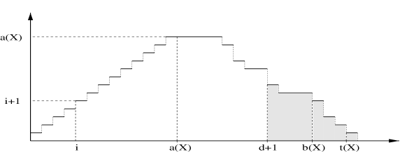
   Figure 2. The graph of a Castelnuovo function (considered as a function on ${\mathbb{R}}_{\geq 0}$ given by ${\mathcal{C}}_{X}(t)={\mathcal{C}}_{X}([t])$). The content of the shaded region is $h^{1}\bigl{(}{\mathcal{J}}_{X/{\mathbb{P}}^{2}}(d)\bigr{)}$.

7. Lemma 1.16 (Davis [Da]).

   Let $X\subset{\mathbb{P}}^{2}$ be a zero-dimensional scheme and $d_{0}\geq a(X)$ such that ${\mathcal{C}}_{X}(d_{0})={\mathcal{C}}_{X}(d_{0}\!+\!1)$. Then there exists a fixed curve $D$ of degree ${\mathcal{C}}_{X}(d_{0})$ in the complete linear system $\big{|}H^{0}\bigl{(}{\mathcal{J}}_{X/{\mathbb{P}}^{2}}(d_{0})\bigr{)}\big{|}$ with the additional property that for each $d\geq 0$ we have ${\mathcal{C}}_{X\cap D}(d)=\min\,\{{\mathcal{C}}_{X}(d),{\mathcal{C}}_{X}(d_{0})\}.$

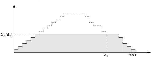
Figure 3. The graph of the Castelnuovo function ${\mathcal{C}}_{X\cap D}$, where $D$ is the fixed curve in $\big{|}H^{0}\bigl{(}{\mathcal{J}}_{X/{\mathbb{P}}^{2}}(d_{0})\bigr{)}\big{|}$ given by Lemma 1.16. The content of the shaded region is $\deg(X\cap D)$.

Definition .

We call a zero-dimensional scheme $X\subset{\mathbb{P}}^{2}$ decomposable if there exists a $d_{0}>0$ such that ${\mathcal{C}}_{X}(d_{0}\!-\!\!\>1)>{\mathcal{C}}_{X}(d_{0})={\mathcal{C}}_{X}(d_{0}\!+\!\!\>1)>0$.

Finally, by Bézout’s Theorem, we have

1. Let $X=C_{d}\cap C_{k}$ be the intersection of two curves $C_{d}$ and $C_{k}$ without common components. Moreover, let $\deg C_{d}=d$, $\deg C_{k}=k$ , $k\leq d$. Then ${\mathcal{C}}_{X}(i)\leq k$ for each $i\geq 0$ and ${\mathcal{C}}_{X}(d+k-i)=i-1$ for any $i=1,\dots,k+1$.

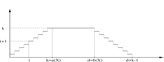
Figure 4. The graph of the Castelnuovo function for the complete intersection $X=C_{d}\cap C_{k}$.

Considering these properties, it is not difficult to prove the following lemma, which is basically due to Barkats [Ba].

Lemma 1.17.

Let $C_{d}\subset{\mathbb{P}}^{2}$ be an irreducible curve of degree $d>0$, and $X\subset C_{d}$ a zero-dimensional scheme such that $h^{1}\bigl{(}{\mathcal{J}}_{X/{\mathbb{P}}^{2}}(d)\bigr{)}>0$. Suppose moreover $d>a(X)$. Then there exists a curve $C_{k}$ of degree $k\geq 3$ such that the scheme $Y=C_{k}\cap X$ is non-decomposable and satisfies

1. $h^{1}\bigl{(}{\mathcal{J}}_{Y/{\mathbb{P}}^{2}}(d)\bigr{)}=h^{1}\bigl{(}{\mathcal{J}}_{X/{\mathbb{P}}^{2}}(d)\bigr{)},$

2. $k_{0}\cdot(d+3-k_{0})\leq\deg Y,$ where $k_{0}=\min\left\{k,\>\left[\tfrac{d+3}{2}\right]\right\}\,.$

Proof. Case 1. Suppose $X$ to be decomposable and let $d_{0}>0$ be maximal with the property ${\mathcal{C}}_{X}(d_{0})={\mathcal{C}}_{X}(d_{0}\!+\!\!\>1)>0.$

By Lemma 1.16, we obtain the existence of a curve $C_{k}$ of degree $k={\mathcal{C}}_{X}(d_{0})<d$ such that $Y:=X\cap C_{k}$ is non-decomposable and ${\mathcal{C}}_{Y}(i)=\min\{{\mathcal{C}}_{X}(i),{\mathcal{C}}_{X}(d_{0})\}$ for each $i\geq 0$. Remark that $Y$ is enclosed in the complete intersection $C_{d}\cap C_{k}$, whence

$$1\>\leq\>{\mathcal{C}}_{Y}(d+1)\>\leq\>{\mathcal{C}}_{C_{k}\cap C_{d}}(d+1)\>=\>k-2\,.$$ (1.8)

In particular, $k\geq 3$ and

$$h^{1}\bigl{(}{\mathcal{J}}_{Y/{\mathbb{P}}^{2}}(d)\bigr{)}\>=\textstyle{\sum\limits_{i=d+1}^{\infty}}{\mathcal{C}}_{Y}(i)\>=\textstyle{\sum\limits_{i=d+1}^{\infty}}{\mathcal{C}}_{X}(i)\>=\>h^{1}\bigl{(}{\mathcal{J}}_{X/{\mathbb{P}}^{2}}(d)\bigr{)}\,.$$

Since $Y$ is non-decomposable and ${\mathcal{C}}_{Y}(i)\leq k$ for each $i\geq 0$, we have

$$\deg Y\>\geq\>\textstyle{\sum\limits_{i=0}^{d+1}}{\mathcal{C}}_{Y}(i)\>\geq\>\textstyle{\sum\limits_{j=1}^{k_{0}}}\bigl{(}d+2-2(j\!-\!1)\bigr{)}\>=\>k_{0}(d+2-k_{0}+1)\,,$$ (1.9)

whence the statement of the lemma.

Case 2. If $X$ is a non-decomposable scheme, we can choose $Y=X$ and $k:=a(X)<d$. By the above reasoning we obtain again (1.8) and (1.9). $\Box$

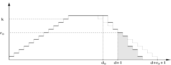
Figure 5. The graph of a Castelnuovo function ${\mathcal{C}}_{Y}$. The content of the shaded region is $h^{1}\bigl{(}{\mathcal{J}}_{Y/{\mathbb{P}}^{2}}(d)\bigr{)}$.

Remark 1.18.

The zero-dimensional scheme $Y$ and the curve $C_{k}$ in Lemma 1.17 satisfy

$$h^{1}\bigl{(}{\mathcal{J}}_{Y/{\mathbb{P}}^{2}}(d)\bigr{)}\>=\,\textstyle{\sum\limits_{i=d+1}^{\infty}}{\mathcal{C}}_{Y}(i)\>\leq\>\tfrac{r_{0}(r_{0}+1)}{2}\,,$$ (1.10)

where $r_{0}:={\mathcal{C}}_{Y}(d+1)\leq k-2$ and (cf. Figure 5)

$$\deg Y = h^{1}\bigl{(}{\mathcal{J}}_{Y/{\mathbb{P}}^{2}}(d)\bigr{)}+\textstyle{\sum\limits_{i=0}^{d}}{\mathcal{C}}_{Y}(i)$$

$$\geq h^{1}\bigl{(}{\mathcal{J}}_{Y/{\mathbb{P}}^{2}}(d)\bigr{)}+\textstyle{\sum\limits_{j=1}^{k_{0}}}(d+r_{0}+1-2(j\!-\!1))-\tfrac{r_{0}(r_{0}+1)}{2}$$

$$= h^{1}\bigl{(}{\mathcal{J}}_{Y/{\mathbb{P}}^{2}}(d)\bigr{)}+(d+2-k_{0}+r_{0})\cdot k_{0}-\tfrac{r_{0}(r_{0}+1)}{2}\,.$$

2. Smoothness

2.1. Equisingular and equianalytic families

Let $S_{1},\dots,S_{r}$ be topological (respectively analytic) types. We recall that, by Proposition 1.1, the variety $V_{d}^{\text{\it irr}}(S_{1},\dots,S_{r})$ is T-smooth at $C\in V_{d}^{\text{\it irr}}(S_{1},\dots,S_{r})$ if and only if

$$h^{1}\bigl{(}{\mathcal{J}}_{X^{\text{es}}(C)/{\mathbb{P}}^{2}}(d)\bigr{)}=0\,,\;\>\bigl{(}\text{respectively }\,h^{1}\bigl{(}{\mathcal{J}}_{X^{\text{ea}}(C)/{\mathbb{P}}^{2}}(d)\bigr{)}=0\bigr{)}\,.$$

In order to formulate our results for the smoothness problem in a short way, we first have to introduce new invariants for plane curve singularities.

Definition .

Let $(C,z)\subset({\mathbb{P}}^{2},z)$ be a reduced plane curve singularity and

$$\emptyset\neq X=X(C,z)\subset X^{\text{ea}}(C,z)$$

be any zero-dimensional scheme. Then we define for any curve germ $(D,z)\subset({\mathbb{P}}^{2},z)$ without common component with $(C,z)$

$$\Delta(C,D;X):=\min\,\bigl{\{}\,(C,D)_{z}-\deg(D\cap X)\,,\;\deg(D\cap X)\,\bigr{\}}\,,$$

where $(C,D)_{z}$ denotes the local intersection number of the germs $(C,z)$ and $(D,z)$. Note that always $\Delta(C,D;X)\geq 1$ (cf. Lemma 4.1 below). Hence, we can introduce

$$\gamma\!\;\bigl{(}C;X\bigr{)}:=\max_{(D,z)}\left\{\tfrac{(\deg(D\cap X))^{2}}{\Delta(C,D;X)}+2\deg(D\cap X)+\Delta(C,D;X)\right\}\,,$$ (2.1)

where the maximum is taken over all curve germs $(D,z)\subset({\mathbb{P}}^{2},z)$ that have no component in common with $(C,z)$. In particular, we introduce

$$\gamma^{\text{es}}\!\>(C,z):=\gamma\!\;\bigl{(}C;\!\>X^{\text{es}}(C,z)\bigr{)}\,\qquad\gamma^{\text{ea}}\!\>(C,z):=\gamma\!\;\bigl{(}C;\!\>X^{\text{ea}}(C,z)\bigr{)}\,.$$

In Section 4 we shall prove the following $h^{1}$-vanishing theorem:

Proposition 2.1.

Let $C\subset{\mathbb{P}}^{2}$ be an irreducible curve of degree $d\geq 6$ with $r$ singular points $z_{1},\dots,z_{r}$ and $X_{i}\subset X^{\text{ea}}(C,z_{i})$, $i=1,\dots,r$, be any zero-dimensional schemes. Moreover, let $X$ be the (disjoint) union of the schemes $X_{1},\dots,X_{r}$. If

$$\textstyle{\sum\limits_{i=1}^{r}}\gamma\!\;(C;X_{i})\,<\,d^{2}+6d+8\,,$$ (2.2)

then $h^{1}\bigl{(}{\mathcal{J}}_{X/{\mathbb{P}}^{2}}(d)\bigr{)}$ vanishes.

As a corollary, we obtain our main smoothness result:

Theorem 1.

Let $C\subset{\mathbb{P}}^{2}$ be an irreducible curve of degree $d\geq 6$ having $r$ singularities $z_{1},\dots,z_{r}$ of topological (respectively analytic) types $S_{1},\dots,S_{r}$ as its only singularities. Then

1. $V_{d}^{\text{\it irr}}(S_{1},\dots,S_{r})$ is T-smooth at $C$ if

   $$\textstyle{\sum\limits_{i=1}^{r}}\gamma^{\text{es}}(C,z_{i})<d^{2}+6d+8\quad\Bigl{(}\text{respectively }\,\textstyle{\sum\limits_{i=1}^{r}}\gamma^{\text{ea}}(C,z_{i})<d^{2}+6d+8\Bigr{)}.$$ (2.3)

2. Under the condition

   $$\textstyle{\sum\limits_{i=1}^{r}}\gamma^{\text{ea}}(C,z_{i})<d^{2}+6d+8$$

   the space of curves of degree $d$ is a joint versal deformation of all singular points of the curve $C$.

In the following lemma we give general estimates for the invariants $\gamma^{\text{es}}(C,z)$ (respectively $\gamma^{\text{ea}}(C,z)$) which show that Theorem 1 improves the previously known results (as stated above):

Lemma 2.2.

For any reduced plane curve singularity $(C,z)\subset({\mathbb{P}}^{2},z)$, we can estimate

$$\gamma^{\text{es}}(C,z)\>\leq(\tau^{\text{es}}(C,z)+1)^{2}\>\text{ and }\>\gamma^{\text{ea}}(C,z)\>\leq(\tau(C,z)+1)^{2}\,,$$

where $\tau(C,z)=\deg X^{\text{ea}}(C,z)$ denotes the Tjurina number, while $\tau^{\text{es}}(C,z)=\deg X^{\text{es}}(C,z)$ is the codimension of the $\mu$-const stratum in a versal deformation base of $(C,z)$.

Proof. Let $(D,z)$ have no common component with $(C,z)$, let $X=X^{\text{es}}(C,z)$ (respectively $X=X^{\text{ea}}(C,z)$) and $\Delta=\Delta(C,D;X)$. There are two cases:

Case 1. $\Delta=\deg D\cap X$. Then, obviously,

$$\tfrac{(\deg(D\cap X))^{2}}{\Delta}+2\deg(D\cap X)+\Delta\>=\>4\cdot\deg(D\cap X)\>\leq\>4\cdot\deg X\>\leq\>(\deg X+1)^{2}.$$

Case 2. $\Delta=(C,D)_{z}-\deg(D\cap X)<\deg(D\cap X)$, i.e., $(C,D)_{z}<2\deg(D\cap X)$. Then

$$\tfrac{(\deg(D\cap X))^{2}}{\Delta}+2\deg(D\cap X)+\Delta\>=\>\tfrac{(C,D)_{z}^{2}}{(C,D)_{z}-\deg(D\cap X)}\,,$$

which is decreasing on $\deg(D\cap X)+1\leq(C,D)_{z}\leq 2\deg(D\cap X)-1$. Consequently, it does not exceed $(\deg(D\cap X)+1)^{2}\leq(\deg X+1)^{2},$ whence the statement. $\Box$

Examples .

1. Let $(C,z)$ be an $A_{k}$-singularity (local equation $x^{2}-y^{k+1}=0$). Then we have $\gamma^{\text{es}}(C,z)=\gamma^{\text{ea}}(C,z)=(k+1)^{2}=(\tau^{\text{es}}(C,z)+1)^{2}$.

2. Let $(C,z)$ be a $D_{4}$-singularity (local equation $x^{3}-y^{3}=0$). Then we obtain (cf. (2.5)) $\gamma^{\text{es}}(C,z)=\gamma^{\text{ea}}(C,z)=18<25=(\tau^{\text{es}}(C,z)+1)^{2}$.

Applying the estimates from Lemma 2.2 to Theorem 1, we obtain in particular:

Corollary 2.3.

Let $d\geq 6$ be an integer. Then $V_{d}^{\text{\it irr}}(S_{1},\dots,S_{r})$ is T-smooth at $C$ if

$$\textstyle{\sum\limits_{i=1}^{r}}\left(\tau^{\text{es}}(C,z)+1\right)^{2}<d^{2}+6d+8\quad\Bigl{(}\text{respectively }\,\textstyle{\sum\limits_{i=1}^{r}}\left(\tau(C,z)+1\right)^{2}<d^{2}+6d+8\Bigr{)}\,.$$

2.2. Families of curves with nodes and cusps

Already for families of curves with nodes and cusps, we obtain a slight improvement against the previously known bounds (cf. [GLS2, Sh5]).

Corollary 2.4.

The variety $V_{d}^{\text{\it irr}}(n\cdot A_{1},\,k\cdot A_{2})$ of irreducible plane curves of degree $d\geq 6$ having $n$ nodes and $k$ cusps as its only singularities is either empty or a smooth variety of the expected dimension $d(d+3)/2-n-2k$ if

$$4n+9k\><\>d^{2}+6d+8\,.$$

Proof. This follows immediately from Theorem 1 (cf. also Corollary 2.3). $\Box$

2.3. Families of curves with ordinary singularities

For families of curves with ordinary singularities (i.e., all local branches are smooth and have different tangents) the new invariants pay off drastically. We obtain a result which is not only asymptotically better than the previously known (cf. [GLS2]), but even asymptotically proper.

Corollary 2.5.

Let $V_{d}^{\text{\it irr}}(m_{1},\dots,m_{r})$ be the variety of irreducible curves of degree $d\geq 6$ having $r$ ordinary multiple points of multiplicities $m_{1},\dots,m_{r}$, respectively, as only singularities. Then $V_{d}^{\text{\it irr}}(m_{1},\dots,m_{r})$ is either empty or a smooth variety of the expected dimension $d(d+3)/2-\sum_{i}\bigl{(}m_{i}(m_{i}\!\!\>+1)/2-2\bigr{)}$ if

$$4\cdot\#(\text{nodes\/})+18\cdot\#(\text{triple points\/})+\textstyle{\sum\limits_{m_{i}\geq 4}}\tfrac{16}{7}\cdot m_{i}^{2}\><\>d^{2}+6d+8.$$ (2.4)

Proof. Let $(C,z)\subset({\mathbb{P}}^{2},z)$ be an ordinary $m$-fold point, then $I^{\text{es}}:=I^{\text{es}}(C,z)=j(C,z)+\mathfrak{m}_{z}^{m}$. We shall show that

$$\max_{(D,z)}\left\{\tfrac{\left(\deg(D\cap X^{\text{es}})+\Delta^{\text{es}}(C,D)\right)^{2}}{\Delta^{\text{es}}(C,D)}\right\}\>=\>\gamma^{\text{es}}(C,z)\>\left\{\begin{array}[]{ll}=4&\text{ if }m=2,\\ =18&\text{ if }m=3,\\ \leq\tfrac{16}{7}m^{2}&\text{ if }m\geq 4,\end{array}\right.$$ (2.5)

whence (2.4) implies (2.3) and the statement follows from Theorem 1. Let $D=(D,z)$ be any plane curve germ of multiplicity $\operatorname{mt}D$ having no common component with $(C,z)$. As before, we have to consider two cases:

Case 1. $\Delta^{\text{es}}(C,D)=\deg(D\cap X^{\text{es}})$. Then

$$\gamma^{\text{es}}(C,z)\>=\>4\deg(D\cap X^{\text{es}})\>\leq\>4\deg X^{\text{es}}\>=\>2m(m+1)-8\,,$$

with equality if $\operatorname{mt}D\geq m$.

Case 2. $\Delta^{\text{es}}(C,D)=(C,D)_{z}-\deg(D\cap X^{\text{es}})<\deg(D\cap X^{\text{es}})$. Note that for fixed $\operatorname{mt}D$ and fixed $\deg(D\cap X^{\text{es}})$ the function

$$\gamma\bigl{(}(C,D)_{z}\bigr{)}:=\tfrac{\left(\deg(D\cap X^{\text{es}})+\Delta^{\text{es}}(C,D)\right)^{2}}{\Delta^{\text{es}}(C,D)}\>=\>\tfrac{(C,D)_{z}^{2}}{(C,D)_{z}-\deg(D\cap X^{\text{es}})}$$

takes its maximum on $\bigl{[}m\cdot\operatorname{mt}D,\,2\deg(D\cap X^{\text{es}})\bigr{]}$ at $(C,D)_{z}=m\cdot\operatorname{mt}D$. Hence, it is not difficult to see that it suffices to consider the cases

Case 2a. $m>\operatorname{mt}D=1$, $(C,D)_{z}=m$. Then $\deg(D\cap X^{\text{es}})=m-1$ and it follows that $\gamma\bigl{(}(C,D)_{z}\bigr{)}=m^{2}$.

Case 2b. $m>\operatorname{mt}D=2$, $(C,D)_{z}=2m$. Then $\deg(D\cap X^{\text{es}})=2(m-1)$, which implies that $\gamma\bigl{(}(C,D)_{z}\bigr{)}=2m^{2}$.

Case 2c. $m\geq\operatorname{mt}D\geq 3$, $m>3$, $(C,D)_{z}=m\cdot\operatorname{mt}D$. Then

$$\deg(D\cap X^{\text{es}}) \leq \dim_{{\mathbb{C}}}({\mathcal{O}}_{D,z}\big{/}\mathfrak{m}_{z}^{m})-1\>=\>\tfrac{m(m+1)}{2}-\tfrac{(m-\operatorname{mt}D)(m-\operatorname{mt}D+1)}{2}-1$$

$$= m\cdot\operatorname{mt}D-\tfrac{(\operatorname{mt}D)^{2}-\operatorname{mt}D+2}{2}\,,$$

which implies that

$$\gamma\bigl{(}(C,D)_{z}\bigr{)}\>\leq\>\tfrac{2(m\cdot\operatorname{mt}D)^{2}}{(\operatorname{mt}D)^{2}-\operatorname{mt}D+2}\>=\>2m^{2}\cdot\tfrac{(\operatorname{mt}D)^{2}}{(\operatorname{mt}D)^{2}-\operatorname{mt}D+2}\>\leq\>\tfrac{16}{7}\cdot m^{2}\,.$$

$\Box$

3. Irreducibility

3.1. Equisingular and equianalytic families

Let $S_{1},\dots,S_{r}$ be topological (respectively analytic) types. Moreover, let $\nu^{\prime}=\nu^{s}$ (resp. $\nu^{a}$) denote the deformation-determinacy as introduced in Section 1.2 (respectively 1.4) and $\tau^{\prime}=\tau^{\text{es}}$ (resp. $\tau^{\prime}=\tau$) denote the codimension of the $\mu$-const stratum in the base of the semiuniversal deformation (respectively the Tjurina number). Our main result on the irreducibility problem is:

Theorem 2.

If $d$ is a positive integer such that $\max_{i}\,\nu^{\prime}(S_{i})\leq\tfrac{2}{5}d-1$ and

$$\textstyle{\sum\limits_{i=1}^{r}}\left(\nu^{\prime}(S_{i})+2\right)^{2} < \tfrac{9}{10}d^{2}\,,$$ (3.1)

$$\tfrac{25}{2}\cdot\#(\text{nodes\/})+18\cdot\#(\text{cusps\/})+\textstyle{\sum\limits_{\tau^{\prime}(S_{i})\geq 3}}\left(\tau^{\prime}(S_{i})+2\right)^{2} < d^{2}$$ (3.2)

then $V_{d}^{\text{\it irr}}(S_{1},\dots,S_{r})$ is irreducible or empty.

In particular, by Lemma 1.5 respectively Remark 1.14, we obtain the following, slightly weaker statement.

Corollary 3.1.

If $d$ is a positive integer satisfying $\,\max_{i}\tau^{\prime}(S_{i})\leq\tfrac{2}{5}d-1\,$ and

$$\tfrac{25}{2}\cdot\#(\text{nodes\/})+18\cdot\#(\text{cusps\/})+\tfrac{10}{9}\cdot\textstyle{\sum\limits_{\tau^{\prime}(S_{i})\geq 3}}(\tau^{\prime}(S_{i})\!+\!2)^{2}<d^{2}$$

then $V_{d}^{\text{\it irr}}(S_{1},\dots,S_{r})$ is irreducible or empty.

Method of proof. To be able to treat both, equisingular (es) and equianalytic (ea), families simultaneously, we introduce

$$X(C):=\left\{\begin{array}[]{cl}X^{s}(C)&\text{ in the ``es''-case}\,,\\ X^{a}(C)&\text{ in the ``ea''-case}\,,\end{array}\right.\;\;\,\text{and}\;\;\,X^{\prime}_{\text{fix}}(C):=\left\{\begin{array}[]{cl}X^{\text{es}}_{\text{fix}}(C)&\text{ in the ``es''-case}\,,\\ X^{\text{ea}}_{\text{fix}}(C)&\text{ in the ``ea''-case}\,.\end{array}\right.$$

Without restriction, we can assume that the types $S_{1},\dots,S_{r^{\prime}}$, $r^{\prime}\leq r$, are pairwise distinct and that for any $i=1,\dots,r^{\prime}$ the type $S_{i}$ occurs precisely $r_{i}$ times in $S_{1},\dots,S_{r}$. We introduce

$$\mathcal{M}=\mathcal{M}(S_{1},\dots,S_{r}):=\textstyle{\prod\limits_{i=1}^{r^{\prime}}\text{Sym}^{r_{i}}({\mathbb{P}}^{2}\!\times\!{\mathcal{H}}_{0}(S_{i}))}$$ (3.3)

and consider the two morphisms

$$\Phi_{d}:V_{d}^{\text{\it irr}}(S_{1},\dots,S_{r})\longrightarrow\text{Sym}^{r}{\mathbb{P}}^{2}\,,\quad C\longmapsto(z_{1}\!+\!\ldots\!+\!z_{r})\,,$$

where $(z_{1}\!+\!\ldots\!+\!z_{r})$ is the unordered tuple of the singularities of $C$ (cf. (1.1)), and

$$V_{d}^{\text{\it irr}}(S_{1},\dots,S_{r})\underset{\text{dense}}{\supset}V\stackrel{{\scriptstyle\Psi_{d}}}{{\longrightarrow}}\mathcal{M}\,,\quad C\longmapsto\bigl{[}\bigl{(}z_{i},\tau_{z_{i}0}(X(C,z_{i}))\bigr{)}\bigr{]}_{i=1,..,r}$$

(cf. (1.5), respectively (1.6)). To obtain the irreducibility of $V_{d}^{\text{\it irr}}(S_{1},\dots,S_{r})$ or, equivalently, of $V$, it suffices to prove that the open subvariety

$$V_{\text{\it reg}}^{(2)}\,:=\,\left\{C\in V\,\big{|}\,h^{1}\bigl{(}{\mathcal{J}}_{X(C)/{\mathbb{P}}^{2}}(d)\bigr{)}=0\right\}\,\subset\,V$$

is dense and irreducible.

Step 1. $V_{\text{\it reg}}^{(2)}$ is irreducible.

For any $C\in V_{\text{\it reg}}^{(2)}$, the fibre $\Psi_{d}^{-1}(\Psi_{d}(C))$ is the open dense subset $U$ of the linear system $\big{|}H^{0}\bigl{(}{\mathcal{J}}_{X(C)/{\mathbb{P}}^{2}}(d)\bigr{)}\big{|}$ consisting of irreducible curves $C^{\prime}\in V$ with $X(C^{\prime})=X(C)$. In particular, the fibres of $\Psi_{d}$ are smooth and equidimensional. On the other hand, it follows from Proposition 1.9, respectively Remark 1.11, that $\mathcal{M}$ is irreducible. Hence, it suffices to show that $\Psi_{d}(V_{\text{\it reg}}^{(2)})$ is dense in $\mathcal{M}$. This will be done in Section 5 (cf. Lemma 5.1).

Step 2. $V_{\text{\it reg}}^{(2)}$ is dense in $V$.

By Proposition 1.1(e), we know that

$$V_{\text{\it gen}}\,:=\,\left\{C\in V\>\big{|}\>\text{Sing}\,C\text{ consists of points in general position}\right\}$$

is a dense subset of

$$V_{\text{\it reg}}^{(1)}\,:=\,\bigl{\{}C\in V\,\big{|}\,h^{1}\bigl{(}{\mathcal{J}}_{X^{\prime}_{\text{fix}}(C)/{\mathbb{P}}^{2}}(d)\bigr{)}=0\bigr{\}}\,.$$

Hence, it suffices to show that $V_{\text{\it gen}}$ is a subset of $V_{\text{\it reg}}^{(2)}$ (this will be done by applying a vanishing theorem for generic fat points, cf. Section 5) and that $V_{\text{\it reg}}^{(1)}\subset V$ is dense. The latter statement takes the main part of Section 5 and will be proven by considering the Castelnuovo function associated to $X^{\prime}_{\text{fix}}(C)$ (cf. Section 1.5). $\Box$

3.2. Families of curves with nodes and cusps

Let $V_{d}^{\text{\it irr}}(n\!\!\>\cdot\!\!\>A_{1},k\!\!\>\cdot\!\!\>A_{2})$ be the variety of irreducible curves of degree $d$ having $n$ nodes and $k$ cusps as only singularities. As an immediate corollary of Theorem 2, we obtain:

Corollary 3.2.

Let $d\geq 8$. Then the variety $V_{d}^{\text{\it irr}}(n\!\!\>\cdot\!\!\>A_{1},k\!\!\>\cdot\!\!\>A_{2})$ is irreducible or empty if

$$\tfrac{25}{2}\!\;n+18\!\>k\><\>d^{2}.$$ (3.4)

3.3. Families with ordinary multiple points

Let $V_{d}^{\text{\it irr}}(m_{1},\dots,m_{r})$ be the variety of irreducible curves of degree $d$ having $r$ ordinary multiple points of multiplicities $m_{1},\dots,m_{r}$, respectively, as only singularities.

Corollary 3.3.

Let $\max\,m_{i}\leq\tfrac{2}{5}\!\;d$. Then $V_{d}^{\text{\it irr}}(m_{1},\dots,m_{r})$ is irreducible or empty if

$$\tfrac{25}{2}\cdot\#(\text{nodes\/})+\textstyle{\sum\limits_{m_{i}\geq 3}}\tfrac{m_{i}^{2}(m_{i}+1)^{2}}{4}\><\>d^{2}.$$ (3.5)

Proof. This follows from Theorem 2, since for an ordinary $m_{i}$-tuple point $(C,z_{i})$ we have

$$\tau^{\text{es}}(C,z_{i})+2=\deg X^{\text{es}}_{\text{fix}}(C,z_{i})=\tfrac{m_{i}(m_{i}+1)}{2}\,,\qquad\nu^{s}(C,z_{i})=m_{i}-1\,.$$

$\Box$

3.4. Comments and Example

We discuss here some aspects of the irreducibility problem concerning the asymptotic properness of the results in Theorem 2 and Corollary 3.1. To reach an asymptotically proper sufficient irreducibility condition one should try to improve the results obtained, reducing singularity invariants in the left-hand side of the inequalities, or find examples of reducible ESF with asymptotics of the singularity invariants being as close as possible to that in sufficient conditions.

The classical problem of finding Zariski pairs, i.e., pairs of curves of the same degree and with the same collection of singularities, which have different fundamental groups of the complement in the plane, has immediate relation to the problem discussed. Nori’s theorem [No] states that $\pi_{1}({\mathbb{P}}^{2}\!\setminus\!\!\>C)={\mathbb{Z}}/d{\mathbb{Z}}$ for any curve $C\in V_{d}^{\text{\it irr}}(S_{1},\dots,S_{r})$ with

$$2\cdot\#(\mbox{nodes})+\!\textstyle{\sum\limits_{S_{i}\neq A_{1}}(\deg X^{s}(S_{i})+\delta(S_{i}))\,<\,d^{2}}\ ,$$

where $X^{\text{es}}_{\text{fix}}$ is the zero-dimensional scheme defined in Section 1.1 and $\delta(S_{i})$ is the $\delta$-invariant. One can easily show that the invariants in the left-hand side are $\leq 3\mu$, hence any examples of Zariski pairs must have asymptotics of singularity invariants as in the necessary condition for existence (0.2), but not as in (3.2).

The following proposition shows that an equisingular family can have components of different dimensions, whereas the fundamental groups of the complements of the curves are the same.

Proposition 3.4.

Let $p,d$ be integers satisfying

$$p\geq 15,\quad 6p\!\;<\!\;d\!\;\leq\!\;12p-\tfrac{3}{2}-\sqrt{35p^{2}\!-\!\!\>15p\!\!\;+\!\!\;\tfrac{1}{4}}\ .$$ (3.6)

Then the family $V_{d}^{\text{\it irr}}(6p^{2}\!\cdot\!\!\>A_{2})$ of irreducible curves of degree $d$ with $6p^{2}$ ordinary cusps has components of different dimensions. Moreover, $\pi_{1}({\mathbb{P}}^{2}\!\!\>\setminus\!\!\;C)={\mathbb{Z}}/d{\mathbb{Z}}$ for all $\,C\in V_{d}^{\text{\it irr}}(6p^{2}\!\cdot\!\!\>A_{2})$.

Proof.

Note that (3.6) implies $d^{2}>36p^{2}\!\!\>=6\!\!\>\cdot\!\!\>6p^{2}$. Hence, due to Nori’s theorem (cf. [No]), $\pi_{1}({\mathbb{P}}^{2}\!\!\>\setminus\!\!\;C)={\mathbb{Z}}/d{\mathbb{Z}}$ for all curves $C\in V_{d}^{\text{\it irr}}(6p^{2}\!\cdot\!\!\>A_{2})$. We show that there are (at least) two different components of $V_{d}^{\text{\it irr}}(6p^{2}\!\cdot\!\!\>A_{2})$: by (3.6),

$$6p^{2}<\tfrac{(6p-1)(6p-2)+2}{4}<\tfrac{(d-1)(d-2)+2}{4}\ ,$$

and [Sh2], Theorem 3.3, gives the existence of a nonempty component $V^{\prime}\!$ of $V_{d}^{\text{\it irr}}(6p^{2}\!\cdot\!\!\>A_{2})$ having the expected dimension

$$\dim V^{\prime}=\tfrac{d(d+3)}{2}-12p^{2}$$

(the expected dimension in the construction of [Sh2] follows from the $S$-transversality in [Sh6], Theorem 3.1).

On the other hand, we construct a family $V^{\prime\prime}$ of bigger dimension: let $C_{2p}$, $C_{3p}$, $C^{\prime}_{d-6p}$, $C^{\prime\prime}_{d-6p}$ be generic curves of degrees $2p$, $3p,$ $d\!\!\>-\!\!\>6p$, $d\!\!\>-\!\!\>6p$, respectively. The curve $C_{d}=C^{3}_{2p}C^{\prime}_{d-6p}\!+C^{2}_{3p}C^{\prime\prime}_{d-6p}$ has degree $d$ and $6p^{2}$ ordinary cusps as its only singularities, one at each intersection point in $C_{2p}\cap C_{3p}$. Varying $C_{2p},C_{3p},C^{\prime}_{d-6p},C^{\prime\prime}_{d-6p}$ in the spaces of curves of degrees $2p,\,3p,\,d\!\!\>-\!\!\>6p,\,d\!\!\>-\!\!\>6p$, respectively, we obtain a subfamily $V^{\prime\prime}$ in $V_{d}^{\text{\it irr}}(6p^{2}\!\cdot\!\!\>A_{2})$. Note that the equality

$$C_{d}\,=\,C^{3}_{2p}C^{\prime}_{d-6p}\!\!\>+C^{2}_{3p}C^{\prime\prime}_{d-6p}\,=\,\widehat{C}^{3}_{2p}\widehat{C}^{\prime}_{d-6p}\!\!\>+\widehat{C}^{2}_{3p}\widehat{C}^{\prime\prime}_{d-6p}\,=\,\widehat{C}_{d}$$

with slightly deformed curves $\widehat{C}_{2p},\widehat{C}_{3p},\widehat{C}^{\prime}_{d-6p},\widehat{C}^{\prime\prime}_{d-6p}$ implies

$$C_{2p}=\widehat{C}_{2p},\quad C_{3p}=\widehat{C}_{3p},\quad C^{\prime}_{d-6p}=\widehat{C}^{\prime}_{d-6p},\quad C^{\prime\prime}_{d-6p}=\widehat{C}^{\prime\prime}_{d-6p}\,.$$

Indeed, if $C_{d}=\widehat{C}_{d}$ then they have $6p^{2}$ common cuspidal points belonging to $C_{2p}$ and $\widehat{C}_{2p}$. Hence, by Bézout’s theorem, $C_{2p}=\widehat{C}_{2p}$. The tangent line to $C_{d}=\widehat{C}_{d}$ at each cusp is tangent to both, $C_{3p}$ and $\widehat{C}_{3p}$, that means, the intersection number of $C_{3p}$ and $\widehat{C}_{3p}$ is at least $12p^{2}$, whence $C_{3p}=\widehat{C}_{3p}$. We can conclude that $C_{2p}^{3}(C^{\prime}_{d-6p}\!\!\>-\widehat{C}^{\prime}_{d-6p})=C_{3p}^{2}(\widehat{C}^{\prime\prime}_{d-6p}\!\!\>-C^{\prime\prime}_{d-6p})$ and, due to $d\!\!\>-\!\!\>6p<2p$, that $C^{\prime}_{d-6p}=\widehat{C}^{\prime}_{d-6p}$, $C^{\prime\prime}_{d-6p}=\widehat{C}^{\prime\prime}_{d-6p}$. Therefore, by (3.6),

$$\dim V^{\prime\prime} = \textstyle{\frac{2p(2p+3)}{2}+\frac{3p(3p+3)}{2}+2\cdot\frac{(d-6p)(d-6p+3)}{2}+1}$$

$$= \textstyle{\frac{d(d+3)}{2}-12p^{2}+\left(\frac{d^{2}}{2}-d\left(12p-\frac{3}{2}\right)+\frac{109p^{2}-21p+2}{2}\right)}\>>\>\dim V^{\prime}.$$

∎

4. Proof of Proposition 2.1

Lemma 4.1.

Let $(C,z)$ be a reduced plane curve singularity and let $I\subset\mathfrak{m}_{z}\subset{\mathcal{O}}_{{\mathbb{P}}^{2},z}$ be an ideal containing the Tjurina ideal $I^{\text{ea}}(C,z)$. Then for any $g\in I$

$$\dim_{\mathbb{C}}{\mathcal{O}}_{{\mathbb{P}}^{2},z}/I\><\>\dim_{\mathbb{C}}{\mathcal{O}}_{{\mathbb{P}}^{2},z}/\langle g,C\rangle\>=\>(g,C)_{z}\,.$$

Proof. cf. [Sh5], Lemma 4.1. $\Box$

Let $C$ be an irreducible curve of degree $d$ having precisely $r$ singularities $z_{1},\dots,z_{r}$ and let

$$X=X_{1}\cup\ldots\cup X_{r}\,,\quad X_{i}\subset X^{\text{ea}}(C,z_{i})\,,$$

$i=1,\dots,r$. Note that for any $i=1,\dots,r$ there exists a curve germ $(D,z_{i})$ containing the scheme $X_{i}$ and satisfying $\Delta(C,D;X_{i})=\deg X_{i}$ (take any $(D,z_{i})$ of sufficiently high multiplicity). Hence, we can estimate

$$\gamma(C;X_{i})\>\geq\>\tfrac{\left(\deg X_{i}+\Delta(C,D;X_{i})\right)^{2}}{\Delta(C,D;X_{i})}\>=\>4\deg X_{i}\,.$$ (4.1)

In particular, by condition (2.2) and since $d\geq 6$, we obtain

$$\deg X\,\leq\,\textstyle{\sum\limits_{i=1}^{r}}\tfrac{1}{4}\cdot\gamma(C;X_{i})\,<\,\tfrac{d^{2}+6d+8}{4}\,\leq\,\tfrac{d(d+1)}{2}\,,$$

whence $d>a(X)=\min\,\big{\{}j\>\big{|}\>h^{0}\bigl{(}{\mathcal{J}}_{X/{\mathbb{P}}^{2}}(j)\bigr{)}>0\big{\}}$. We want to show that $h^{1}\bigl{(}{\mathcal{J}}_{X/{\mathbb{P}}^{2}}(d)\bigr{)}$ vanishes. Assume that this is not the case, that is,

$$h^{1}\bigl{(}{\mathcal{J}}_{X/{\mathbb{P}}^{2}}(d)\bigr{)}>0\,.$$

Then Lemma 1.17 gives the existence of a curve $D$ of degree $k\geq 3$ such that $Y=D\cap X$ is non-decomposable and satisfies $h^{1}\bigl{(}{\mathcal{J}}_{Y/{\mathbb{P}}^{2}}(d)\bigr{)}=h^{1}\bigl{(}{\mathcal{J}}_{X/{\mathbb{P}}^{2}}(d)\bigr{)}>0$. Moreover, by (4.1) and (2.2), we have

$$\deg Y\>=\>\deg(X\cap D)\><\>\tfrac{(d+3)^{2}}{4}-\tfrac{1}{4}\>\leq\>\left[\tfrac{d+3}{2}\right]\cdot\left(d+3-\left[\tfrac{d+3}{2}\right]\right)\,.$$ (4.2)

Hence, by Lemma 1.17, $k=k_{0}<\left[\tfrac{d+3}{2}\right]$ and

$$\deg Y\>\geq\>k\cdot(d+3-k)\,.$$ (4.3)

Consequently, we can even estimate $k$ as

$$k\>\leq\>\tfrac{d+3}{2}-\sqrt{\tfrac{(d+3)^{2}}{4}-\deg Y}\>=\>\tfrac{2\cdot\deg Y}{d+3+\sqrt{(d+3)^{2}-4\deg Y}}\,.$$ (4.4)

On the other hand, let $Y=Y_{1}\cup\ldots\cup Y_{s}$, $\#Y:=s$, be the decomposition of the zero-dimensional scheme $Y$ into its irreducible components (without loss of generality, we may assume that $Y_{i}$ is supported at $z_{i}$ for $i=1,\dots,s\leq r$). Note that, due to Lemma 4.1, we have

$$\deg Y_{i}\,\leq\,(C,D)_{z_{i}}-\Delta_{i}\,,\quad\Delta_{i}\geq 1\,,$$

which, together with (4.3) implies

$$k\cdot d\>\geq\>\textstyle{\sum\limits_{i=1}^{s}}(C,D)_{z_{i}}\>\geq\>\deg Y+\textstyle{\sum\limits_{i=1}^{s}}\Delta_{i}\>\geq\>k\cdot(d+3-k)+\textstyle{\sum\limits_{i=1}^{s}}\Delta_{i}\,.$$

Thus, by (4.4), we can estimate

$$\textstyle{\sum\limits_{i=1}^{s}}\Delta_{i}\>\leq\>k(k-3)\><\>k^{2}\>\leq\>\Bigl{(}\tfrac{2\cdot\deg Y}{d+3+\sqrt{(d+3)^{2}-4\deg Y}}\Bigr{)}^{2}\,.$$

In particular, applying the Cauchy inequality, we obtain

$$\textstyle{\sum\limits_{i=1}^{s}}\tfrac{(\deg Y_{i})^{2}}{\Delta_{i}}\>\geq\>\tfrac{(\deg Y)^{2}}{\Delta_{1}+\ldots+\Delta_{s}}\>>\>\tfrac{1}{4}\Bigl{(}1+\sqrt{1-\tfrac{4\deg Y}{(d+3)^{2}}}\>\Bigr{)}^{2}\!\cdot(d+3)^{2}\,.$$ (4.5)

Now, we introduce

$$\alpha_{Y}:=\frac{\sum_{i=1}^{s}\frac{(\deg Y_{i})^{2}}{\Delta_{i}}}{(d+3)^{2}}\,,\quad\beta_{Y}:=\frac{\sum_{i=1}^{s}\frac{(\deg Y_{i})^{2}}{\Delta_{i}}}{\deg Y}\,.$$

Then (4.5) implies that

$$\alpha_{Y}>\tfrac{1}{4}\cdot\Bigl{(}1+\sqrt{1-4\!\>\tfrac{\alpha_{Y}}{\beta_{Y}}}\>\Bigr{)}^{2},\quad\text{ i.e., }\>\alpha_{Y}>\Bigl{(}\tfrac{\beta_{Y}}{\beta_{Y}+1}\Bigr{)}^{2}.$$

Finally, we have

$$(d+3)^{2} = \tfrac{\beta_{Y}}{\alpha_{Y}}\cdot\deg Y\><\>\bigl{(}1+\tfrac{1}{\beta_{Y}}\bigr{)}^{2}\cdot\beta_{Y}\cdot\deg Y\>=\>\bigl{(}\beta_{Y}+2+\tfrac{1}{\beta_{Y}}\bigr{)}\cdot\deg Y$$

$$\leq \textstyle{\sum\limits_{i=1}^{s}}\Bigl{(}\tfrac{(\deg Y_{i})^{2}}{\Delta_{i}}+2\cdot\deg Y_{i}+\Delta_{i}\Bigr{)}\>\leq\>\textstyle{\sum\limits_{i=1}^{s}}\gamma(C;X_{i})\,,$$

which contradicts (2.2). $\Box$

5. Proof of Theorem 2

In this section, we complete the proof of Theorem 2. To do so, using the notations introduced in Section 3.1, we shall prove the following lemmas:

Lemma 5.1.

If $V_{\text{\it reg}}^{(2)}$ is non-empty then $\Psi_{d}(V_{\text{\it reg}}^{(2)})$ is dense in $\mathcal{M}$.

Lemma 5.2.

Let $C\in V_{d}^{\text{\it irr}}(S_{1},\dots,S_{r})$ be a curve that has its singularities in generic position $z_{1},\dots,z_{r}$. If $\,2d>5\cdot\max_{i}\nu^{\prime}(C,z_{i})+4\,$ and

$$\tfrac{9}{10}\cdot(d+3)^{2}>\textstyle{\sum\limits_{i=1}^{r}}\bigl{(}\nu^{\prime}(C,z_{i})+2\bigr{)}^{2},$$ (5.1)

then $h^{1}\bigl{(}{\mathcal{J}}_{X(C)/{\mathbb{P}}^{2}}(d)\bigr{)}$ vanishes, that is, $V_{\text{\it gen}}$ is a subset of $V_{\text{\it reg}}^{(2)}$.

Lemma 5.3.

Let $d\geq 8$ be an integer and $C\in V_{d}^{\text{\it irr}}(S_{1},\dots,S_{r})$ such that

$$d^{2}+6d+8 > 4\,\deg X^{\prime}_{\text{fix}}(C)\,,$$ (5.2)

$$d^{2} > \textstyle{\sum\limits_{i=1}^{r}}(\deg X^{\prime}_{\text{fix}}(C,z_{i}))^{2},$$ (5.3)

$$2\cdot(d+3)^{2} > \textstyle{\sum\limits_{i=1}^{r}}(\deg X^{\prime}_{\text{fix}}(C,z_{i})+2)^{2},$$ (5.4)

$$\tfrac{9}{10}\cdot d^{2} > \textstyle{\sum\limits_{i=1}^{r}}\max\,\bigr{\{}\,\bigl{(}\deg D\cap X^{\prime}_{\text{fix}}(C,z_{i})\bigr{)}^{2}\,\big{|}\>D\text{ a smooth curve}\,\bigr{\}},$$ (5.5)

$$(d-1)^{2} > \textstyle{\sum\limits_{i=1}^{r}}\max\,\left(\begin{array}[]{c}\bigl{\{}\,\bigl{(}\deg D\cap X^{\prime}_{\text{fix}}(C,z_{i})\bigr{)}^{2}\,\big{|}\>D\text{ a smooth curve}\,\bigr{\}}\\ \cup\>\bigl{\{}\,\tfrac{1}{2}\cdot\bigl{(}\deg X^{\prime}_{\text{fix}}(C,z_{i})\bigr{)}^{2}\,\bigr{\}}\end{array}\right),$$ (5.8)

$$\tfrac{16}{15}\cdot(d+3)^{2} > \textstyle{\sum\limits_{i=1}^{r}}\max\,\left(\begin{array}[]{c}\bigl{\{}\,\bigl{(}\deg D\cap X^{\prime}_{\text{fix}}(C,z_{i})+\tfrac{16}{15}\bigr{)}^{2}\,\big{|}\>D\text{ a smooth curve}\,\bigr{\}}\\ \cup\>\bigl{\{}\,\tfrac{1}{2}\cdot\bigl{(}\deg X^{\prime}_{\text{fix}}(C,z_{i})+\textstyle{\frac{32}{15}}\bigr{)}^{2}\,\bigr{\}}\end{array}\right).$$ (5.11)

Then $V_{\text{\it reg}}^{(1)}$ is dense in $V$ ,i.e., $h^{1}\bigl{(}{\mathcal{J}}_{X^{\prime}_{\text{fix}}(C)/{\mathbb{P}}^{2}}(d)\bigr{)}=0$ for generic $C\in V$.

Remark 5.4.

Note that for any reduced plane curve singularity $(C,z)\subset({\mathbb{P}}^{2},z)$ and any smooth curve germ $D$ at $z$ we have

$$\deg X^{\prime}_{\text{fix}}(C,z)\>=\>\tau^{\prime}(C,z)+2\>\geq\>\nu^{\prime}(C,z)+2\,,\quad\deg\bigl{(}D\cap X^{\prime}_{\text{fix}}(C,z)\bigr{)}\>\leq\>\nu^{\prime}(C,z)+1\,.$$

For instance, in the case of nodes and cusps, we have

$$\deg X^{\prime}_{\text{fix}}(C,z)=\left\{\begin{array}[]{ll}3&\text{ for a node},\\ 4&\text{ for a cusp},\end{array}\right.\qquad\nu^{\prime}(C,z)=\left\{\begin{array}[]{ll}1&\text{ for a node},\\ 2&\text{ for a cusp},\end{array}\right.$$

$$\max\,\bigl{\{}\!\>\deg(D\cap X^{\prime}_{\text{fix}}(C,z))\>\big{|}\>D\text{ smooth}\,\bigr{\}}\,=\,\left\{\begin{array}[]{ll}2&\text{ for a node},\\ 3&\text{ for a cusp}.\end{array}\right.$$

Hence, it is not difficult to see that the conditions (3.2) and (3.1) imply (5.2)–(5.11).

Proof of Lemma 5.1. By Sections 1.2, 1.4, we know that for any $i=1,\dots,r$ there exists an $m_{i}$ such that the schemes $X(C,z_{i})$, depend only on the $(m_{i}\!-\!1)$-jet of the equation of $(C,z_{i})$. Hence, for $d_{0}\geq\max\,m_{i}$ the morphism $\Psi_{d_{0}}$ is dominant. Moreover, we can assume $d_{0}$ to be sufficiently large such that $h^{1}\bigl{(}{\mathcal{J}}_{X(C)/{\mathbb{P}}^{2}}(d_{0})\bigr{)}$ vanishes. Hence,

$$\dim\,\mathcal{M} = \dim\Psi_{d_{0}}(V)\>=\>\dim V_{d_{0}}(S_{1},\dots,S_{r})-h^{0}\bigl{(}{\mathcal{J}}_{X(C)/{\mathbb{P}}^{2}}(d_{0})\bigr{)}+1$$

$$= \dim V_{d_{0}}(S_{1},\dots,S_{r})-\tfrac{d_{0}(d_{0}+3)}{2}+\deg X(C)\,.$$

On the other hand, let $C\in V_{\text{\it reg}}^{(2)}$. Then the vanishing of $h^{1}\bigl{(}{\mathcal{J}}_{X(C)/{\mathbb{P}}^{2}}(d)\bigr{)}$ implies in particular the T-smoothness of $V_{d}(S_{1},\dots,S_{r})$ at $C$ (cf. Proposition 1.1 (c)). Hence, as an open subvariety, $V_{\text{\it reg}}^{(2)}$ is also smooth at $C$ of the expected codimension

$$\tfrac{d(d\!\!\;+\!\!\;3)}{2}-\dim V_{\text{\it reg}}^{(2)}\>=\>\tfrac{d_{0}(d_{0}\!\!\>+\!\!\;3)}{2}-\dim V_{d_{0}}(S_{1},\dots,S_{r})\,,$$

that is,

$$\dim\Psi_{d}(V_{\text{\it reg}}^{(2)}) = \dim V_{\text{\it reg}}^{(2)}-h^{0}\bigl{(}{\mathcal{J}}_{X(C)/{\mathbb{P}}^{2}}(d)\bigr{)}+1\>=\>\dim V_{\text{\it reg}}^{(2)}-\tfrac{d(d+3)}{2}+\deg X(C)$$

$$= \dim V_{d_{0}}(S_{1},\dots,S_{r})-\tfrac{d_{0}(d_{0}+3)}{2}+\deg X(C)\>=\>\dim\mathcal{M}\,,$$

whence the statement. $\Box$

Proof of Lemma 5.2. Let $i\in\{1,\dots,r\}$ and $\nu_{i}=\nu^{\prime}(C,z_{i})$. By definition of $\nu_{i}$, the scheme $X(C,z_{i})$ is contained in the ordinary fat point given by the ideal $\mathfrak{m}_{z_{i}}^{\nu_{i}+1}$. Hence it suffices to show that $h^{1}\bigl{(}{\mathcal{J}}_{Y(\nu_{1}+1,\dots,\nu_{r}+1)/{\mathbb{P}}^{2}}(d)\bigr{)}=0\,,$ where $Y(\nu_{1}\!+\!1,\dots,\nu_{r}\!+\!1)$ is the zero-dimensional scheme of $r$ ordinary fat points of multiplicities $\nu_{1}\!+\!1,\dots,\nu_{r}\!+\!1$ in general position. Now, the statement follows from [Xu], Theorem 3. $\Box$

Proof of Lemma 5.3. Assume $V$ has an irreducible component $V^{\ast}\!\subset V\backslash V_{\text{\it reg}}^{(1)}$, that is, the generic element $C$ of $V^{\ast}$ satisfies

$$h^{1}\bigl{(}{\mathcal{J}}_{X^{\prime}_{\text{fix}}(C)/{\mathbb{P}}^{2}}(d)\bigr{)}>0\,.$$

We denote by $\Sigma^{\ast}\subset\text{Sym}^{r}{\mathbb{P}}^{2}=:\Sigma$ the closure of $\Phi_{d}(V^{\ast})$.

Recall that the dimension of $\Phi_{d}^{-1}\bigl{(}\Phi_{d}(C)\bigr{)}$ at $C$ is just the dimension of $V_{d,\text{fix}}(S_{1},\dots,S_{r})$ at $C$, that is, by Proposition 1.1 (b),

$$\dim\Phi_{d}^{-1}\bigl{(}\Phi_{d}(C)\bigr{)}\>\leq\>h^{0}\bigl{(}{\mathcal{J}}_{X^{\prime}_{\text{fix}}(C)/{\mathbb{P}}^{2}}(d)\bigr{)}-1\,.$$

To obtain the statement of Lemma 5.3, it suffices to show that under the given (numerical) conditions we would have

$$h^{1}\bigl{(}{\mathcal{J}}_{X^{\prime}_{\text{fix}}(C)/{\mathbb{P}}^{2}}(d)\bigr{)}<\>\text{codim}_{\Sigma}\Sigma^{\ast},$$ (5.12)

because this would imply that

$$\dim V^{\ast} \leq \dim\Sigma^{\ast}+h^{0}\bigl{(}{\mathcal{J}}_{X^{\prime}_{\text{fix}}(C)/{\mathbb{P}}^{2}}(d)\bigr{)}-1$$

$$< \dim\Sigma+h^{0}\bigl{(}{\mathcal{J}}_{X^{\prime}_{\text{fix}}(C)/{\mathbb{P}}^{2}}(d)\bigr{)}-h^{1}\bigl{(}{\mathcal{J}}_{X^{\prime}_{\text{fix}}(C)/{\mathbb{P}}^{2}}(d)\bigr{)}-1\,=\,\dim V_{\text{\it reg}}^{(1)}\,,$$

whence a contradiction (any component of $V$ has at least the expected dimension $\dim V_{\text{\it reg}}^{(1)}$).

Step 1. For $d\geq 6$ the condition (5.2) implies in particular that $\deg X^{\prime}_{\text{fix}}(C)\leq d(d\!\!\>+\!\!\>1)/2$, whence $d>a(X^{\prime}_{\text{fix}}(C))=\min\,\bigl{\{}i\,\big{|}\,h^{0}\bigl{(}{\mathcal{J}}_{X^{\prime}_{\text{fix}}(C)/{\mathbb{P}}^{2}}(i)\bigr{)}>0\bigr{\}}$. By Lemma 1.17, we obtain the existence of a curve $C_{k}$ of degree $k\geq 3$ such that the subscheme $Y=C_{k}\cap X^{\prime}_{\text{fix}}(C)\subset C_{k}\cap C$ is non-decomposable with

$$h^{1}\bigl{(}{\mathcal{J}}_{Y/{\mathbb{P}}^{2}}(d)\bigr{)}\,=\,h^{1}\bigl{(}{\mathcal{J}}_{X^{\prime}_{\text{fix}}(C)/{\mathbb{P}}^{2}}(d)\bigr{)}\>\leq\>\tfrac{r_{0}(r_{0}+1)}{2}\,,$$ (5.13)

where $1\leq r_{0}:={\mathcal{C}}_{X^{\prime}_{\text{fix}}(C)}(d+1)\leq k-2$ (cf. Remark 1.18). Since, by (5.2), we suppose additionally that

$$\deg Y\><\>\left[\tfrac{d+3}{2}\right]\cdot\left(d+3-\left[\tfrac{d+3}{2}\right]\right),$$ (5.14)

we have $k<\left[\tfrac{d+3}{2}\right]$ and (cf. Lemma 1.17 and Remark 1.18)

$$\deg Y\>\geq\>\max\left\{k\cdot(d\!+\!3\!-\!k)\,,\;\>k\cdot(d\!+\!2\!+\!r_{0}\!-\!k)+h^{1}\bigl{(}{\mathcal{J}}_{Y/{\mathbb{P}}^{2}}(d)\bigr{)}-\tfrac{r_{0}(r_{0}+1)}{2}\right\}\,.$$ (5.15)

Now, we can estimate the codimension of $\Sigma^{\ast}$ in $\Sigma$. Given the curve $C_{k}$, the number of conditions on $X^{\prime}_{\text{fix}}(C)$ imposed by fixing the support of the subscheme $Y=C_{k}\cap X^{\prime}_{\text{fix}}(C)$ on $C_{k}$ respectively its singular locus is at least $\#Y$ if $C_{k}$ is non-reduced and at least $\#Y+\#(Y|_{\text{Sing}\,C_{k}})$ if $C_{k}$ is a reduced curve. On the other hand, the dimension of the variety of reduced (respectively non reduced) curves $C_{k}$ of degree $k$ is given by $h^{0}\bigl{(}{\mathcal{O}}_{{\mathbb{P}}^{2}}(k)\bigr{)}-1$ (respectively $h^{0}\bigl{(}{\mathcal{O}}_{{\mathbb{P}}^{2}}(k\!\!\>-\!\!\>2)\bigr{)}+2$). Thus, in place of (5.12), it suffices to show that

$$h^{1}\bigl{(}{\mathcal{J}}_{Y/{\mathbb{P}}^{2}}(d)\bigr{)}\><\>\min\,\left\{\#Y-\tfrac{k^{2}-k}{2}-2\,,\;\#Y+\#(Y|_{\text{Sing}\,C_{k}})-\tfrac{k(k+3)}{2}\right\}\,.$$ (5.16)

Step 2. Recall that we have $k\geq 3$ and, by (5.13),

$$h^{1}\bigl{(}{\mathcal{J}}_{X^{\prime}_{\text{fix}}(C)/{\mathbb{P}}^{2}}(d)\bigr{)}\>=\>h^{1}\bigl{(}{\mathcal{J}}_{Y/{\mathbb{P}}^{2}}(d)\bigr{)}\>\leq\>\tfrac{(k-2)(k-1)}{2}\,.$$ (5.17)

Step 2a. Assume $\,h:=h^{1}\bigl{(}{\mathcal{J}}_{Y/{\mathbb{P}}^{2}}(d)\bigr{)}=\tfrac{(k-2)(k-1)}{2}$.

Note that this implies that the Castelnuovo functions of $Y$ and $C_{k}\cap C$ coincide, in particular we have $\deg Y=kd$, i.e., $Y=C_{k}\cap C$. In this case the condition (5.16) is satisfied whenever

$$0\><\>\min\,\left\{\#Y-k^{2}+2k-3\,,\;\#Y+\#(Y|_{\text{Sing}\,C_{k}})-k^{2}-1\right\}\,.$$ (5.18)

Now, we have to consider two cases

Case 1: $\#(Y|_{\text{Sing}\,C_{k}})\geq 1$. Then the right-hand side is bounded from below by $\#Y-k^{2}=\#Y-(\deg Y)^{2}/d^{2},$ whence, due to the Cauchy inequality, it suffices to have

$$d^{2}\>>\>\textstyle{\sum\limits_{i=1}^{r}}\deg(\underbrace{X^{\prime}_{\text{fix}}(C,z_{i})\cap C_{k}}_{\displaystyle{=:Y_{i}}})^{2},$$ (5.19)

which is implied by (5.3).

Case 2: $\#(Y|_{\text{Sing}\,C_{k}})=0$. Then, as $k\geq 3$, the right-hand side is bounded from below by $\#Y-k^{2}-1\geq\#Y-\tfrac{10}{9}k^{2}$, whence (5.18) holds whenever

$$\textstyle{\sum\limits_{i=1}^{r}}(\deg Y_{i})^{2}\><\>\tfrac{9}{10}\,d^{2}\;\text{ with }\;\deg Y_{i}\>\leq\>\max\,\left\{\deg D\cap X^{\prime}_{\text{fix}}(C,z_{i})\mid D\text{ smooth}\right\}\,,$$

which is a consequence of (5.5).

Step 2b. Assume $h=h^{1}\bigl{(}{\mathcal{J}}_{Y/{\mathbb{P}}^{2}}(d)\bigr{)}<\tfrac{(k-2)(k-1)}{2}\,,$ in particular $k\geq 4$.

As we have seen in (5.16), it suffices to show that

$$\max_{k,h}\,\Bigl{\{}h+\underbrace{\tfrac{k^{2}-k}{2}+2}_{\displaystyle=:p_{1}(k)}\Bigr{\}}\><\>\#Y\;\,\text{ and }\;\,\max_{k,h}\,\Bigl{\{}h+\!\!\underbrace{\tfrac{k(k+3)}{2}}_{\displaystyle=:p_{2}(k)}\Bigr{\}}\><\>\#Y+\#(Y|_{\text{Sing}\,C_{k}})\,.$$ (5.20)

We introduce

$$\rho_{j}\>:=\>\min\,\bigg{\{}\tfrac{(\deg Y)^{2}}{p_{j}(k)+h}\;\Big{|}\;\begin{array}[]{l}1\leq h\leq\min\,\bigl{\{}\tfrac{r_{0}(r_{0}+1)}{2},\,\tfrac{k(k-3)}{2}\bigr{\}}\\ 4\leq k\,,\;1\leq r_{0}\leq k-2\end{array}\bigg{\}}\,,\qquad j=1,2\,.$$

By the Cauchy inequality, it follows that (5.20) holds whenever

$$\textstyle{\sum\limits_{i=1}^{s}}(\deg Y_{i})^{2}\><\>\rho_{1}\;\,\text{ and }\textstyle{\sum\limits_{z_{i}\not\in\text{Sing}\,C_{k}}}(\deg Y_{i})^{2}\,+\textstyle{\sum\limits_{z_{i}\in\text{Sing}\,C_{k}}}\tfrac{(\deg Y_{i})^{2}}{2}\><\>\rho_{2}\,.$$ (5.21)

It remains to estimate $\rho_{1}$ and $\rho_{2}$ as functions in $d$. By (5.15), we have for any $j=1,2$

$$\tfrac{(\deg Y)^{2}}{p_{j}(k)+h}\>\geq\>\tfrac{\left(2k(d+2-k+r_{0})+2h-r_{0}(r_{0}+1)\right)^{2}}{4(p_{j}(k)+h)}=:f_{j}(k,h,r_{0})\,,$$

that is,

$$\rho_{j}\>\geq\>\min\,\bigg{\{}f_{j}(k,h,r_{0})\;\Big{|}\;\begin{array}[]{l}1\leq h\leq\min\,\bigl{\{}\tfrac{r_{0}(r_{0}+1)}{2},\,\tfrac{k(k-3)}{2}\bigr{\}}\\ 4\leq k\,,\;1\leq r_{0}\leq k-2\,.\end{array}\bigg{\}}\,,\qquad j=1,2\,.$$

Remark that for fixed $k,h$ the functions $f_{j}(k,h,\underline{\phantom{H}}\,)$ are increasing in $r_{0}$ (on $\bigl{[}0,k-\tfrac{1}{2}\bigr{]}$). Hence, they take their minima for the minimal possible value, that is, for $r_{0}$ satisfying

$$\left(\,\tfrac{r_{0}(r_{0}+1)}{2}=h\,,\;\>r_{0}\leq k-3\,\right)\;\text{ or }\;\left(\,r_{0}=k-2\,,\;\>h\geq\tfrac{(k-3)(k-2)}{2}+1\,\right)\,.$$

Case 1: $r_{0}=k-2$, $k(k-3)\geq 2h\geq(k-3)(k-2)+2$. In this case we can estimate

$$f_{j}(k,h,r_{0})\>\geq\>\tfrac{\left(2kd+(k-3)(k-2)+2-(k-2)(k-1)\right)^{2}}{4p_{j}(k)+2k(k-3)}\>=\>\tfrac{2\left(kd-k+3\right)^{2}}{2p_{j}(k)+k(k-3)}\,,$$

whence, due to $k\leq(d+3)/2$,

$$f_{1}(k,h,r_{0}) \geq \tfrac{(kd-k+3)^{2}}{k^{2}-2k+2}\>\geq\>\tfrac{k^{2}(d-1)^{2}}{k^{2}-2k+2}\>=\>d^{2}+\tfrac{d^{2}(2k-2)-k^{2}(2d-1)}{k^{2}-2k+2}\>\geq\>d^{2}\,,$$

$$f_{2}(k,h,r_{0}) \geq \left(d-1+\tfrac{3}{k}\right)^{2}\>\geq\>(d-1)^{2}\,.$$

Thus, (5.21) is a consequence of (5.3) and (5.8).

Case 2: $h=r_{0}(r_{0}+1)/2$, $r_{0}\leq k-3$. It follows that

$$f_{j}(k,h,r_{0})\>\geq\>\tfrac{2k^{2}(d+2-k+r_{0})^{2}}{2p_{j}(k)+r_{0}(r_{0}+1)}\,=:\,g_{j}(k,r_{0})\,,\quad j=1,2\,.$$

We fix $k\geq 4$, and look for the minimum of $g_{j}(k,r_{0})$. Since the derivative

$$\tfrac{\partial}{\partial r_{0}}\,g_{j}(k,r_{0})\>=\>\underbrace{\tfrac{2k^{2}(d+2-k+r_{0})}{(2p_{j}(k)+r_{0}(r_{0}+1))^{2}}}_{>0}\,\cdot\,\bigl{(}\,r_{0}(\underbrace{\phantom{\big{|}}\!\!2k-2d-3}_{<0})+4p_{j}(k)+k-d-2\,\bigr{)}$$

changes sign at most once (from positive to negative), the minimum of $g_{j}(k,r_{0})$ is taken at one of the endpoints, that is,

$$\rho_{j}\>\geq\>\min\,\{g_{j}(k,1),\,g_{j}(k,k-3)\}\,,\quad j=1,2\,.$$

We have $\,g_{1}(k,1)=\tfrac{2k^{2}}{k^{2}-k+6}\cdot(d+3-k)^{2}\,$ and $\,g_{2}(k,1)=\tfrac{2k^{2}}{k^{2}+3k+2}\cdot(d+3-k)^{2}$. Recall that due to (5.15) we can estimate

$$d+3-k\>\geq\>\tfrac{d+3}{2}+\sqrt{\tfrac{(d+3)^{2}}{4}-\deg Y}\,,$$

whence we obtain

$$g_{1}(k,1)\>\geq\>\left\{\begin{array}[]{ll}\displaystyle\min\,\bigl{\{}\,\tfrac{16}{9}\!\;(d-1)^{2},\;\,\tfrac{25}{13}\!\;(d-2)^{2}\,\bigr{\}}&\text{ if }k\in\{4,5\}\\ \displaystyle\tfrac{1}{2}\!\>\bigl{(}\,d+3+\sqrt{(d+3)^{2}-4\deg Y}\>\bigr{)}^{2}&\text{ if }k\geq 6\end{array}\right.$$

and

$$g_{2}(k,1)\>\geq\>\tfrac{4}{15}\!\>\bigl{(}\,d+3+\sqrt{(d+3)^{2}-4\deg Y}\>\bigr{)}^{2}\,.$$

On the other hand, we have $k<(d+3)/2$, which implies that

$$g_{1}(k,k-3)\>=\>\tfrac{k^{2}(d-1)^{2}}{k^{2}-3k+5}\>>\>d^{2}\,\>\text{ and }\>\,g_{2}(k,k-3)\>=\>\tfrac{k^{2}(d-1)^{2}}{k^{2}-k+3}\>>\>(d-1)^{2}.$$ (5.22)

Thus, if (5.3) and (5.8) are satisfied and $d\geq 8$, the condition (5.21) holds whenever

$$\textstyle{\sum\limits_{i=1}^{s}}(\deg Y_{i})^{2}\><\>\tfrac{1}{2}\!\>\bigl{(}\,d+3+\sqrt{(d+3)^{2}-4\deg Y}\>\bigr{)}^{2}$$ (5.23)

and

$$\textstyle{\sum\limits_{z_{i}\not\in\text{Sing}\,C_{k}}}(\deg Y_{i})^{2}+\textstyle{\sum\limits_{z_{i}\in\text{Sing}\,C_{k}}}\tfrac{(\deg Y_{i})^{2}}{2}\><\>\tfrac{4}{15}\bigl{(}\,d+3+\sqrt{(d+3)^{2}-4\deg Y}\>\bigr{)}^{2}.$$ (5.24)

Step 3. In the following, we analyse the conditions (5.23) and (5.24). We write $\sum\frac{(\deg Y_{i})^{2}}{\varepsilon_{i}}$ to denote the left-hand side of (5.23) respectively (5.24). As above, we introduce the numbers

$$\alpha_{Y,\varepsilon}\>:=\>\frac{\sum_{i=1}^{s}\frac{(\deg Y_{i})^{2}}{\varepsilon_{i}}}{(d+3)^{2}}\,,\quad\beta_{Y,\varepsilon}\>:=\>\frac{\sum_{i=1}^{s}\frac{(\deg Y_{i})^{2}}{\varepsilon_{i}}}{\deg Y}$$ (5.25)

and look for the possible values of $\alpha_{Y,\varepsilon}$ such that (5.23), respectively (5.24), holds. This is the case whenever

$$\alpha_{Y,\varepsilon}\><\>\tfrac{K}{4}\cdot\left(\,1+\sqrt{1-4\tfrac{\alpha_{Y,\varepsilon}}{\beta_{Y,\varepsilon}}}\>\right)^{2},$$

where $K=2$, respectively $K=16/15$, that is, if

$$\textstyle{\sum\limits_{i=1}^{s}}\tfrac{(\deg Y_{i})^{2}}{\varepsilon_{i}}\>=\>\alpha_{Y,\varepsilon}\cdot(d+3)^{2}\><\>\tfrac{K\cdot\beta_{Y,\varepsilon}^{2}}{(\beta_{Y,\varepsilon}+K)^{2}}\cdot(d+3)^{2}\,.$$

Note that this restriction can be reformulated as

$$\left(\textstyle{\sum_{i=1}^{s}}\tfrac{(\deg Y_{i})^{2}}{\varepsilon_{i}}\right)\cdot\left(1+\tfrac{K}{\beta_{Y,\varepsilon}}\right)^{2}\;<\;K(d+3)^{2},$$

where, by the Cauchy inequality, the left-hand side can be estimated as

$$\left(\textstyle{\sum\limits_{i=1}^{s}}\tfrac{(\deg Y_{i})^{2}}{\varepsilon_{i}}\right)\cdot\Bigl{(}1+\tfrac{K}{\beta_{Y,\varepsilon}}\Bigr{)}^{2} = \frac{\left(\sum_{i=1}^{s}\frac{(\deg Y_{i})^{2}}{\varepsilon_{i}}+K\cdot\sum_{i=1}^{s}\deg Y_{i}\right)^{2}}{\sum_{i=1}^{s}\frac{(\deg Y_{i})^{2}}{\varepsilon_{i}}}$$

$$\leq \textstyle{\sum\limits_{i=1}^{r}}\tfrac{\left(\deg Y_{i}+K\cdot\varepsilon_{i}\right)^{2}}{\varepsilon_{i}}\,.$$

Finally, since $Y_{i}\subset X^{\prime}_{\text{fix}}(C,z_{i})$, the conditions (5.23) and (5.24) are satisfied if we suppose (5.4) and (5.11). $\Box$

References

- [Ba] Barkats, D.: Irréductibilité des variétés des courbes planes à noeuds et à cusps. Preprint Univ. de Nice-Sophia-Antipolis (1993).
- [BG] Buchweitz, R.-O.; Greuel, G.-M.: The Milnor number and deformations of complex curve singularities. Invent. math. 58, 241–281 (1980).
- [Br] Briançon, J.: Description de Hilb. Invent. math. 41, 45–89 (1977).
- [Ca] Casas-Alvero, E.: Infinitely near imposed singularities and singularities of polar curves. Math. Ann. 287, 429–454 (1990).
- [CS] Chiantini, L.; Sernesi, E.: Nodal curves on surfaces of general type. Math. Ann. 307, 41–56 (1997).
- [Da] Davis, E.D.: 0-dimensional subschemes of : New applications of Castelnuovo’s function. Ann. Univ. Ferrara, Vol. 32, 93–107 (1986).
- [DH] Diaz, S.; Harris, J.: Ideals associated to deformations of singular plane curves. Trans. Amer. Math. Soc. 309, 433–468 (1988).
- [Fo] Fogarty, J.: Algebraic families on an algebraic surface. Amer. J. Math. 90, 511–521 (1968).
- [GK] Greuel, G.-M.; Karras, U.: Families of varieties with prescribed singularities. Compos. math. 69, 83–110 (1989).
- [GL] Greuel, G.-M.; Lossen, C.: Equianalytic and equisingular families of curves on surfaces. Manuscr. math. 91, 323–342 (1996).
- [GLS] Greuel, G.-M.; Lossen, C.; Shustin, E.: Geometry of families of nodal curves on the blown-up projective plane. Trans. Amer. Math. Soc. 350, 251–274 (1998).
- [GLS1] Greuel, G.-M.; Lossen, C.; Shustin, E.: Plane curves of minimal degree with prescribed singularities. Invent. Math. 133, 539–580 (1998).
- [GLS2] Greuel, G.-M.; Lossen, C.; Shustin, E.: New asymptotics in the geometry of equisingular families of curves. Int. Math. Res. Not. 13, 595–611 (1997).
- [GPS] Greuel, G.-M.; Pfister, G.; Schönemann, H.: Singular version 1.2 User Manual. In: Reports On Computer Algebra, number 21. Centre for Computer Algebra, University of Kaiserslautern, (1998). http://www.mathematik.uni-kl.de/~zca/Singular.
- [Ha] Hartshorne, R.: Connectedness of the Hilbert scheme. Publ. Math. de IHES 29, 261–304 (1966).
- [Ia] Iarrobino, A.: Punctual Hilbert schemes. Mem. Amer. Math. Soc., No. 188 (1977).
- [Ia1] Iarrobino, A.: Hilbert scheme of points: Overview of last ten years. Proceed. of Symposia in Pure Math. 46, 297–320 (1987).
- [Li] Lichtin, B.: Estimates and formulae for the degree of sufficiency of plane curves. Singularities, Part 2 (Arcata 1981). Proceed. of Symposia in Pure Math. 40, 155–160 (1983).
- [Lo] Lossen, C.: New asymptotics for the existence of plane curves with prescribed singularities. To appear in Commun. in Algebra (1999).
- [Lo1] Lossen, C.: The Geometry of equisingular and equianalytic families of curves on surfaces. Thesis, Univ. Kaiserslautern (1998).
- [MY] Mather, J.N.; Yau S. S.-T.: Classification of isolated hypersurface singularities by their moduli algebras. Invent. math. 69, 243–251 (1982).
- [No] Nori, M.: Zariski conjecture and related problems. Ann. Sci. Ec. Norm. Sup. (4) 16, 305-344 (1983).
- [NV] Nobile, A.; Villamayor, O.E.: Equisingular stratifications associated to families of planar ideals. J. Algebra 193, No. 1, 239–259 (1997).
- [Ri] Risler, J.-J.: Sur les deformations équisingulières d’idéaux. Bull. Soc. math. France 101, 3–16 (1973).
- [Se] Severi, F.: Vorlesungen über algebraische Geometrie. Teubner (1921) resp. Johnson (1968).
- [Sh] Shustin, E.: Versal deformation in the space of plane curves of fixed degree. Function. Anal. Appl. 21, 82–84 (1987).
- [Sh1] Shustin, E.: On manifolds of singular algebraic curves. Selecta Math. Sov. 10, 27–37 (1991).
- [Sh2] Shustin, E.: Real plane algebraic curves with prescribed singularities. Topology 32, 845–856 (1993).
- [Sh3] Shustin, E.: Smoothness and irreducibility of varieties of algebraic curves with nodes and cusps. Bull. SMF 122, 235–253 (1994).
- [Sh4] Shustin, E.: Geometry of equisingular families of plane algebraic curves. J. Algebraic Geom. 5, 209–234 (1996).
- [Sh5] Shustin, E.: Smoothness of equisingular families of plane algebraic curves. Int. Math. Res. Not. 2, 67–82 (1997).
- [Sh6] Shustin, E.: Gluing of singular and critical points. Topology 37, no. 1, 195-217 (1998).
- [Te] Teissier, B.: The hunting of invariants in the geometry of discriminants. In P. Holm, Real and Complex Singularities, Oslo 1976, Northholland (1978).
- [Wa] Wahl, J.: Equisingular deformations of plane algebroid curves. Trans. Amer. Math. Soc. 193, 143–170 (1974).
- [Xu] Xu, Geng: Ample line bundles on smooth surfaces. J. reine angew. Math. 469, 199–209 (1995).
- [Za] Zariski, O.: Algebraic Surfaces. 2nd ed. Springer, Berlin etc. (1971).