Random Matrices and Random Permutations

Abstract

We prove the conjecture of Baik, Deift, and Johansson which says that with respect to the Plancherel measure on the set of partitions $\lambda$ of $n$, the rows $\lambda_{1},\lambda_{2},\lambda_{3},\dots$ of $\lambda$ behave, suitably scaled, like the 1st, 2nd, 3rd, and so on eigenvalues of a Gaussian random Hermitian matrix as $n\to\infty$. Our proof is based on an interplay between maps on surfaces and ramified coverings of the sphere. We also establish a connection of this problem with intersection theory on the moduli spaces of curves.

1 Introduction

1.1 Plancherel measures

The Plancherel measure is probability measure defined on the set $G^{\wedge}$ of irreducible representations $\pi$ of any finite group $G$. Concretely, the measure of a representation $\pi$ is $(\dim\pi)^{2}\big{/}|G|$. It is called Plancherel because the Fourier transform

$$L^{2}(G,\mu_{\mathrm{Haar}})^{G}\xrightarrow{\quad Fourier\quad}L^{2}(G^{\wedge},\mu_{\mathrm{Plancherel}})$$

is an isometry just like in the classical Plancherel theorem.

In this paper we will be dealing with Plancherel measures for $S(n)$ and their asymptotics as $n\to\infty$. The set $S(n)^{\wedge}$ is labeled by partitions $\lambda$ of $n$ or, equivalently, by Young diagrams with $n$ squares. We denote the Plancherel measure by

$$\mathfrak{P}_{n}(\lambda)=\frac{(\dim\lambda)^{2}}{n!}\,,\quad|\lambda|=n\,,$$

and recall that the dimension $\dim\lambda$ is given by several classical formulas such as the hook formula.

1.2 Limit shape

Logan and Shepp [33] and, independently, Vershik and Kerov [40] (see also the paper [41] which contains complete proofs of the results announced in [40]) discovered the following measure concentration phenomenon for the Plancherel measures for $S(n)$ as $n\to\infty$. Take a diagram $\lambda$, scale it in both directions by a factor of $n^{-1/2}$ so that to obtain a shape of unit area, and rotate it by $135^{\circ}$ like in Figure 1.

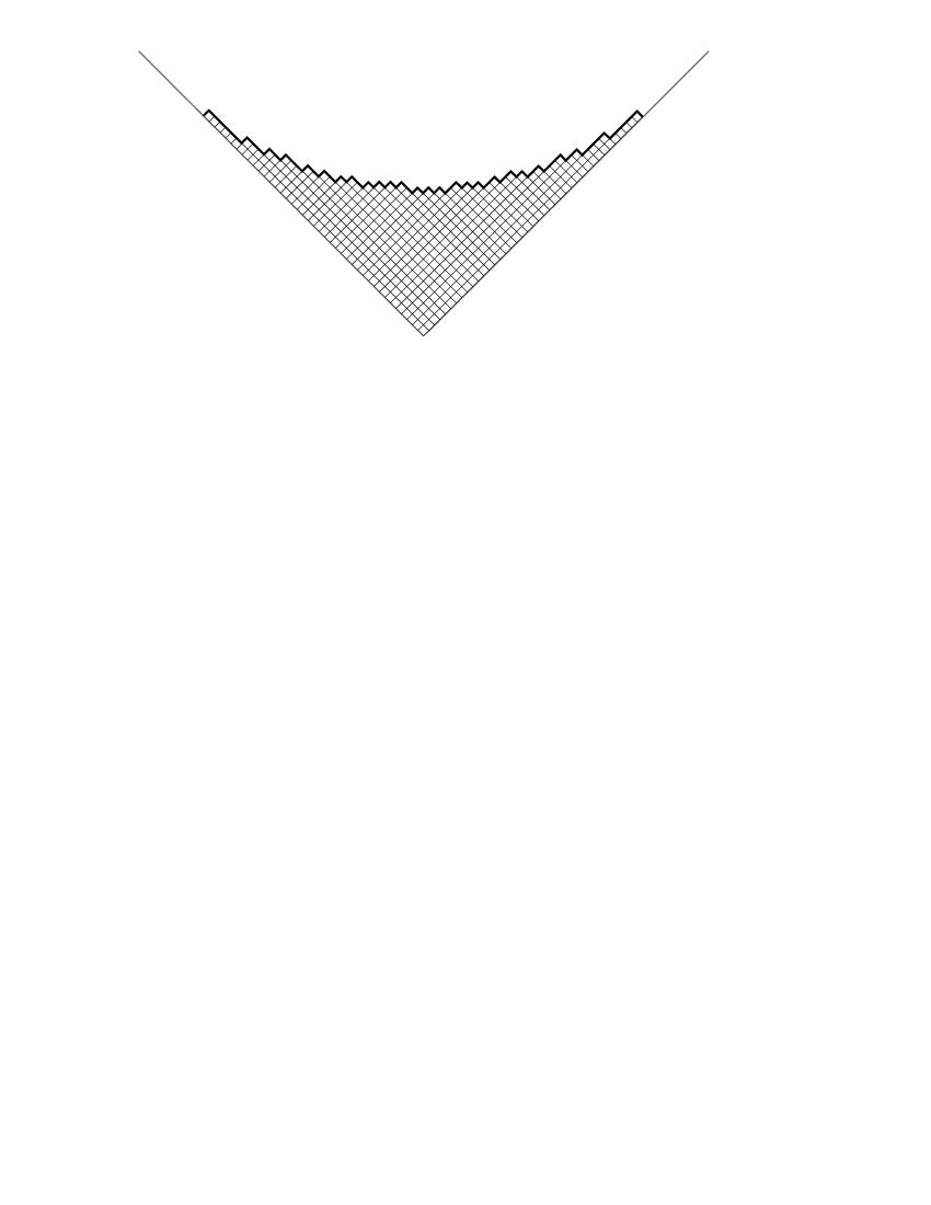
Figure 1: A Young diagram rotated $135^{\circ}$

The boundary of this shape is a polygonal line which is thickened in Figure 1. In this way the Plancherel measure $\mathfrak{P}$ becomes a measure on the space of continuous functions. It was shown in [33, 40, 41] that as $n\to\infty$, this measure converges to the delta measure at the following function

$$\Omega(x)=\begin{cases}\frac{2}{\pi}\left(x\arcsin(x/2)+\sqrt{4-x^{2}}\right)&|x|\leq 2,\\ |x|&|x|\geq 2\,,\end{cases}$$ (1.1)

whose graph is drawn in Figure 2.

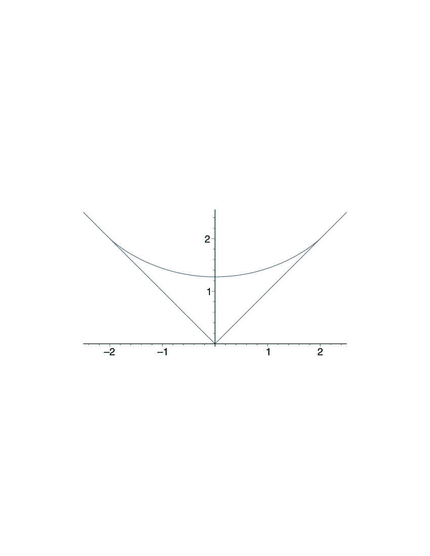
Figure 2: The limit curve $\Omega(x)$

The constant 2 in (1.1) means that the first part of $\lambda$ should behave like $\sim 2\sqrt{n}$ as $n\to\infty$. Indeed, it was shown in [40, 41] that $\lambda_{1}/\sqrt{n}\to 2$ in probability (in [33] the inequality $\lim\lambda_{1}/\sqrt{n}\geq 2$ was obtained). This constant 2 corresponds to the constant 2 in the Ulam problem about the length of the longest increasing subsequence in a random permutation; it was also obtained by different means in [1, 16, 36]. About the history of the Ulam problem see [1, 2] and vast literature cited there.

1.3 CLT for limit shape

The next term in the asymptotic of the Plancherel measure was computed by Kerov in [20] who showed that the Plancherel measure behaves like

$$\Omega(x)+\frac{U(x)}{n^{1/2}}+o\left(\frac{1}{n^{1/2}}\right)\,,n\to\infty\,,$$ (1.2)

where $U(x)$ is the following Gaussian random process

$$U(x)=\sum_{k=1}^{\infty}\zeta_{k}\,\frac{U_{k}(x)}{\sqrt{k+1}}\,.$$

Here $U_{k}(x)$ are the Tchebychef polynomials of the second kind

$$U_{k}(2\cos\phi)=\frac{\sin(k+1)\phi}{\sin\phi}$$

and $\zeta_{k}$ are independent standard normal variables. Observe that near the endpoints $x=\pm 2$ the formula (1.2) becomes inadequate because the series diverges at the endpoints. For more information about the behavior of the Plancherel typical partition in the bulk of the limit shape the reader is referred to the recent paper [8].

1.4 Edge of the limit shape and Baik-Deift-Johansson conjecture

The behavior of the Plancherel measure near the edges of $[-2,2]$ has been the subject of intense recent studies and numerical experiments, see [2] and references therein. It has been conjectured by Baik, Deift, and Johansson that this behavior, suitably scaled, is identical to the behavior of the eigenvalues of a random Hermitian matrix near the edge of the Wigner semicircle. More precisely, consider a random $n\times n$ matrix

$$H=\left(\begin{array}[]{ccc}&\vdots&\\ \ldots&h_{ij}&\ldots\\ &\vdots&\end{array}\right)_{1\leq i,j\leq n}\,,\quad h_{ij}=\overline{h_{ji}}$$

such that the real and imaginary parts

$$h_{ij}=u_{ij}+iv_{ij}$$

are independent normal variables with mean 0 and variance $1/2$. Let

$$E_{1}\geq E_{2}\geq E_{3}\geq\dots$$

be the eigenvalues of $H$. Introduce the variables $y_{i}$

$$y_{i}=n^{2/3}\left(\frac{E_{i}}{2n^{1/2}}-1\right)\,,\quad i=1,2,\dots\,.$$ (1.3)

Then as $n\to\infty$ the $y_{i}$’s have a limit distribution which was studied in [13, 39] and other papers. In particular, the correlation functions of this random point process have determinantal form with the Airy kernel, see for example [39]. The distributions of individual $y_{i}$’s were obtained by Tracy and Widom in [39]; they involve certain solutions of the Painlevé II equation.

Similarly, let $\lambda=(\lambda_{1},\lambda_{2},\dots)$ be a partition and set (note the difference with (1.3) in the exponent of $n$)

$$x_{i}=n^{1/3}\left(\frac{\lambda_{i}}{2n^{1/2}}-1\right)\,,\quad i=1,2,\dots\,.$$ (1.4)

Baik, Deift, and Johansson conjectured that the limit distribution of the $x_{i}$’s exists and coincides with that of the $y_{i}$’s. They verified this conjecture for the distribution of $x_{1}$ and $x_{2}$ in [2] and [3], respectively, using very advanced analytic methods.

1.5 Main result

The aim of this paper is to give a direct combinatorial proof of proof of the following result.

Consider the points $x_{1},x_{2},\dots$ as a random measure on $\mathbb{R}$ with masses 1 placed at the points $x_{i}$, $i=1,2,\dots$. Consider its Laplace transform

$$\widehat{x}(\xi)=\sum_{i=1}^{\infty}\exp(\xi x_{i})\,,\quad\xi>0\,,$$

this is a random process on $\mathbb{R}_{>0}$. Define $\widehat{y}(\xi)$ similarly. Denote expectation by angle brackets.

Theorem 1

In the $n\to\infty$ limit, all mixed moments of the random variables $\widehat{x}(\xi)$ exist and are identical to those of $\widehat{y}(\xi)$, that is,

$$\lim_{n\to\infty}\Big{\langle}\,\widehat{x}(\xi_{1})\cdots\widehat{x}(\xi_{s})\,\Big{\rangle}=\lim_{n\to\infty}\Big{\langle}\,\widehat{y}(\xi_{1})\cdots\widehat{y}(\xi_{s})\,\Big{\rangle}\,,$$ (1.5)

for any $s=1,2,\dots$ and any numbers $\xi_{1},\dots,\xi_{s}>0$.

From Theorem 1 one obtains the following result about the distribution of the individual rows of a Plancherel typical partition $\lambda$

Theorem 2

In the $n\to\infty$ limit, the joint distribution of $x_{1},\dots,x_{k}$ is identical to the joint distribution of $y_{1},\dots,y_{k}$ for any fixed $k$.

1.6 Maps on surfaces vs.  branched coverings

In our proof of Theorem 1 we use the equivalence of two points of view on topological surfaces (or algebraic curves). One way to think about a surface is to imagine it glued from polygons by identifying sides of polygons in pairs. Such a representation is a combinatorial structure called a map on a surface. In connection with quantum gravity, it has been long known that maps are most intimately related to random matrices, see e. g. [42] for an elementary introduction.

Another equally classical way of representing a surface is to realize it as a ramified covering the sphere $S^{2}$, or in other words, as a Riemann surface of an algebraic function of one complex variable. It is classically known that every problem about the combinatorics of covering has a translation into a problem about permutations which arise as monodromies around the ramification points.

The two sides of (1.5) have a combinatorial interpretation as asymptotics of certain maps and coverings, respectively. We produce a correspondence between the two enumeration problems and show that its deviation from being a bijection is negligible in the $n\to\infty$ limit.

1.7 Connection to moduli spaces of curves

The two sides of (1.5) are also very directly connected to intersection theory on the moduli spaces $\overline{\mathcal{M}}_{g,s}$ of genus $g$ curves with $s$ marked points. Namely, we show in Section 2.5.5 that our enumeration problem for maps (or coverings) is related to Kontsevich’s combinatorial model [19] for intersection numbers on $\overline{\mathcal{M}}_{g,s}$ by, essentially, a reparametrization.

This reparametrization involves passage times for the standard Brownian motion. As a consequence, our enumeration asymptotics derived in Theorem 3, differs from the unique boxed formula of [19] by replacing the Laplace transform variables by their square roots.

It follows that the limit (1.5) is a close relative of the so called $s$-point function for the intersection numbers of the $\psi$-classes on $\overline{\mathcal{M}}_{g,s}$. This can be used to compute the $s$-point function, see [31].

It is tempting to speculate that both sides of (1.5) must be certain Riemann integral sums for the corresponding integrals over $\overline{\mathcal{M}}_{g,s}$ and the only difference between them is that one discretizes $\overline{\mathcal{M}}_{g,s}$ using maps and the other — using coverings.

For another application of asymptotics of coverings to evaluation of integrals over certain moduli spaces see [11]. Another connection between coverings and moduli spaces was obtained in [12].

1.8 Jucys-Murphy elements

The reader would be hardly surprised to learn that our main technical tool on the symmetric group side are the Jucys–Murphy elements [18, 27, 9]. In recent years, they have become all–purpose heavy–duty technical tools in representation theory of $S(n)$, see for example [5, 25, 28, 29, 32]. The observation that in the $n\to\infty$ the spectral measures (in the regular representation) of these elements becomes the Wigner semicircle was made by P. Biane in [4].

1.9 Historic remarks

The existence of a connection between Plancherel measures and random matrices has been actively advocated by S. Kerov, see e.g. [21, 22, 23]. The simplest evidence of such a connection is the fact that the so called transition distribution for the limit shape $\Omega$ coincides with the Wigner semicircle. Random matrices also enter the representation theory of symmetric groups via the free probability theory. For a detailed discussion of the interplay between symmetric groups and free probability see the paper [5] by P. Biane. Our results explain, at least to some extend, this connection.

1.10 Further development

An analytic proof of the Baik–Deift–Johansson conjecture was found subsequently in [8] and, independently, in [17]. This approach is based on an exact formula for the so-called correlation functions of the poissonized Plancherel measure. Same formula allows to analyze the local structure of a Plancherel typical partition in the bulk of the limit shape, see [8]. This exact formula for correlation functions is a special case of the result obtained in [7]. The results of [7] were considerably generalized in [30].

1.11 Acknowledgements

The author would like to thank A. Eskin for numerous discussions and P. Biane for explaining the connection to Brownian motion. The author was supported by NSF for under grant DMS–9801466.

2 Random Matrices

2.1 Maps on surfaces and Random Matrices

2.1.1

The relation between maps on surfaces and random matrices via the Wick formula is well known. Classical examples of exploiting this relation are, for example, the papers [15, 19]. A very accessible introduction can be found, for example, in [42]. See also, for example, [14] for a physical survey. We briefly recall some basic things in order to facilitate the comparison with the enumeration of coverings.

2.1.2

Consider a random Hermitian matrix

$$H=\left(\begin{array}[]{ccc}&\vdots&\\ \ldots&h_{ij}&\ldots\\ &\vdots&\end{array}\right)_{1\leq i,j\leq n}\,,\quad h_{ij}=\overline{h_{ji}}$$

such that the real and imaginary parts

$$h_{ij}=u_{ij}+iv_{ij}$$

are independent normal variables with mean 0 and variance $1/2$. We will be interested in the asymptotics of

$$\frac{1}{2^{|k|}n^{|k|/2}}\left\langle{\prod_{j=1}^{s}\operatorname{tr}H^{k_{i}}}\right\rangle\,,\quad k_{i}\sim\xi_{j}n^{2/3}$$ (2.1)

as $n\to\infty$ and some fixed $\xi_{1},\dots,\xi_{s}>0$. Here $|k|=\sum_{i}k_{i}$. Similar averages were considered by many authors, see especially the recent paper [38] and references therein. Remark that by (1.3) we have

$$\left(\frac{E_{i}}{2n^{1/2}}\right)^{\xi_{j}n^{2/3}}\to\exp(\xi_{j}y_{i})\,,\quad n\to\infty\,,$$

and that it is clear that only the eigenvalues near the edges of the Wigner’s semicircle contribute to the asymptotics of (2.1).

2.1.3

By symmetry, the expectation (2.1) vanishes if $|k|$ is odd. If $|k|$ is even then then it is a sum of $2^{s-1}$ terms coming from various combinations of the maximal and minimal eigenvalues of $H$. In what follows, we will always assume that $|k|$ is even. In this case, there are $2^{s-1}$ possible choices of parity of each individual $k_{i}$ and it is easy to see that by taking a suitable linear combination we can single out the contribution of only maximal eigenvalues. Therefore, instead of working with expectations like

$$\Big{\langle}\,\widehat{y}(\xi_{1})\cdots\widehat{y}(\xi_{s})\,\Big{\rangle}$$ (2.2)

we can work with expectations (2.1) which is more convenient.

2.1.4 Correlation functions

Let $\boldsymbol{\varrho}(x_{1},\dots,x_{k})$ denote the $k$-point correlation functions for the scaled eigenvalues $\dfrac{E_{i}}{2\sqrt{n}}$ of $H$. The expectations (2.1) are closely related to these correlation functions. Let

$$\boldsymbol{\sigma}=\sum_{i}\delta_{E_{i}/2\sqrt{n}}\,,$$

be the scaled spectral measure of $H$. It is a random measure on $\mathbb{R}$. We have

$$\frac{1}{2^{|k|}n^{|k|/2}}\left\langle{\prod_{j=1}^{s}\operatorname{tr}H^{k_{i}}}\right\rangle=\int_{\mathbb{R}^{s}}u_{1}^{k_{1}}\dots u_{s}^{k_{s}}\,\left\langle{\boldsymbol{\sigma}^{\times s}}\right\rangle(du)$$ (2.3)

where $\left\langle{\boldsymbol{\sigma}^{\times s}}\right\rangle$ is the following nonrandom measure on $\mathbb{R}^{s}$

$$\left\langle{\boldsymbol{\sigma}^{\times s}}\right\rangle(A_{1}\times\cdots\times A_{s})=\left\langle{\prod_{i=1}^{s}\boldsymbol{\sigma}(A_{i})}\right\rangle\,.$$

Let $\Pi_{s}$ be the set of all partitions of the set $\{1,\dots,s\}$ into disjoint union of subsets. For any $\alpha\in\Pi_{s}$, denote by $\ell(\alpha)$ the number of parts in $\alpha$. For example,

$$\alpha=\{\{1\},\{2,3\}\}\in\Pi_{3}\,,\quad\ell(\alpha)=2\,.$$

For any $k\in\mathbb{R}^{s}$ and $\alpha\in\Pi_{s}$ denote by $k_{\alpha}\in\mathbb{R}^{\ell(\alpha)}$ the vector with coordinates $\sum_{j\in\alpha_{i}}k_{j}$, where $\alpha_{i}$ are the parts of $\alpha$. We have

$$\int_{\mathbb{R}^{s}}u^{k}\,\left\langle{\boldsymbol{\sigma}^{\times s}}\right\rangle(du)=\sum_{\alpha\in\Pi_{s}}\int_{\mathbb{R}^{\ell(\alpha)}}u^{k_{\alpha}}\,\boldsymbol{\varrho}(u_{1},\dots,u_{\ell(\alpha)})\,du\,.$$ (2.4)

For example, for $s=2$ we have

$$\int_{\mathbb{R}^{2}}u_{1}^{k_{1}}u_{2}^{k_{2}}\,\left\langle{\boldsymbol{\sigma}^{\times s}}\right\rangle(du)=\int_{\mathbb{R}^{2}}u_{1}^{k_{1}}u_{2}^{k_{2}}\,\boldsymbol{\varrho}(u_{1},u_{2})\,du_{1}\,du_{2}+\int_{\mathbb{R}^{1}}u_{1}^{k_{1}+k_{2}}\,\boldsymbol{\varrho}(u_{1})\,du_{1}\,.$$

2.1.5 Wick formula

From the Wick formula one obtains

$$\frac{1}{2^{|k|}n^{|k|/2}}\left\langle{\prod_{j=1}^{s}\operatorname{tr}H^{k_{i}}}\right\rangle=\frac{1}{2^{|k|}}\sum_{\mathsf{S}}n^{\chi(\mathsf{S})-s}\,\left|\operatorname{Map}_{\mathsf{S}}(k_{1},\dots,k_{s})\right|\,,$$ (2.5)

where the sum is over all homeomorphism classes of surfaces $\mathsf{S}$, not necessarily connected, $\chi(\mathsf{S})$ is the Euler characteristic of the surface $S$, and $\operatorname{Map}_{\mathsf{S}}(k_{1},\dots,k_{s})$ is the set of solutions to the the following combinatorial problem.

Take $s$ polygons: a $k_{1}$-gon, a $k_{2}$-gon, and so on. Fix their orientations and a mark a vertex on each as in Figure 3 (we mark a vertex to distinguish a $k$-gon from its $(k-1)$ rotations).

Figure 3: Polygons with orientation and marked vertices

Now consider all possible ways to glue their sides in pairs in a way consistent with orientation. The set $\operatorname{Map}_{\mathsf{S}}$ consists of all glueings which produce a surface homeomorphic to $\mathsf{S}$.

Note that definition of a map is different from the more common one which does not require the choice of marked vertices. Our definition is more convenient for our purposes.

2.1.6

We are interested in the limit of (2.5) as $n$ and the $k_{i}$’s go to infinity in such a way that $k_{i}\propto n^{2/3}$. This limit can be determined by taking the term-wise asymptotics in the right-hand side of (2.5).

For $s=1$ the necessary bounds for the validity of term-wise limits will be obtained from explicit formulas in Section 2.6. For $s>1$, we then can use the equation (2.4) and the fact that the correlation functions $\boldsymbol{\varrho}$ have a determinantal form and hence

$$\boldsymbol{\varrho}(u_{1},\dots,u_{k})\leq\prod_{i=1}^{k}\boldsymbol{\varrho}(u_{i})\,.$$ (2.6)

Here we use the well-known fact that the determinant of a positive-definite matrix is at most the product of its diagonal entries (equivalently, the volume of a parallelepiped is at most the product of its side lengths). Consequently, we obtain the estimate (2.32) which says that left-hand side of (2.5) is bounded by some function of the variables $\xi_{i}=k_{i}\,n^{-2/3}$.

Since all terms in the right-hand side of (2.5) are nonnegative, replacing $n$ by a multiple of $n$ we see that the terms in in the right-hand side of (2.5) decay faster than any exponential and, in particular, taking term-wise limit is justified.

2.1.7

Our present goal is to understand the asymptotics of $\left|\operatorname{Map}_{\mathsf{S}}(k_{1},\dots,k_{s})\right|$ as the $k_{i}$’s go to the infinity. It is clear that it suffices to consider this asymptotics for connected surfaces $\mathsf{S}$ only. If $\mathsf{S}$ is a connected surface of genus $g$ we write $\operatorname{Map}_{g}$ instead of $\operatorname{Map}_{\mathsf{S}}$.

Below we will describe a function $\operatorname{map}_{g}(\xi_{1},\dots,\xi_{s})$ such that

$$2^{-|k|}\,\left|\operatorname{Map}_{g}(k_{1},\dots,k_{s})\right|\sim\operatorname{map}_{g}(\xi)\,t^{3g-3+3s/2}\,,\quad\xi_{i}=k_{i}/t\,,$$ (2.7)

as $t\to\infty$ provided $|k|$ is even. Recall that if $|k|$ is odd then $\operatorname{Map}_{g}$ is empty. One extends $\operatorname{map}_{\mathsf{S}}$ to disconnected surfaces multiplicatively. It is clear from (2.7) that $\operatorname{map}_{\mathsf{S}}$ is homogeneous of total degree $\frac{3}{2}(s-\chi(\mathsf{S}))$ and also positive for positive values of $\xi$.

It follows that if all $k_{i}$’s are even then

$$\frac{1}{2^{|k|}n^{|k|/2}}\left\langle{\prod_{j=1}^{s}\operatorname{tr}H^{k_{i}}}\right\rangle\to\sum_{\mathsf{S}}\operatorname{map}_{\mathsf{S}}(\xi_{1},\dots,\xi_{s})\,,\quad k_{i}\sim\xi_{i}\,n^{2/3}\,,$$ (2.8)

and if some of the $k_{i}$’s are odd then in the right-hand side of the above formula those terms that violate the parity conditions should be omitted.

2.1.8

The function $\operatorname{map}_{g}(\xi)$ can be expressed in terms of the Laplace transform of the corresponding limits of the correlation functions $\boldsymbol{\varrho}$.

It is known (see [39] and note that our $y_{i}$’s differ from the centered and scaled eigenvalues which are used in [39] by a factor of 2) that

$$n^{-2s/3}\,\boldsymbol{\varrho}\left(1+\frac{y_{1}}{n^{2/3}},\dots,1+\frac{y_{s}}{n^{2/3}}\right)\to\rho(y_{1},\dots,y_{s})\,,\quad n\to\infty\,,$$ (2.9)

where $\rho$ is given by a determinant

$$\rho(y_{1},\dots,y_{s})=\det\big{(}K(y_{i},y_{j})\big{)}$$

with the Airy kernel

$$K(x,y)=\frac{\operatorname{Ai}(2x)\,\operatorname{Ai}^{\prime}(2y)-\operatorname{Ai}^{\prime}(2x)\operatorname{Ai}(2y)}{x-y}\,.$$

Here $\operatorname{Ai}(x)$ is the classical Airy function. By the l’Hôspital’s rule and the equation $\operatorname{Ai}^{\prime\prime}(x)=x\operatorname{Ai}(x)$, we have

$$K(x,x)=2\operatorname{Ai}^{\prime}(2x)^{2}-4x\operatorname{Ai}(2x)^{2}\,.$$ (2.10)

Denote by $R(\xi)$ the Laplace transform

$$R(\xi_{1},\dots,\xi_{s})=\int_{\mathbb{R}^{s}}e^{(\xi,y)}\,\rho(y_{1},\dots,y_{s})\,dy\,,$$

which converges for all $\xi\in\mathbb{R}_{>0}^{s}$. Introduce the function

$$H(\xi_{1},\dots,\xi_{s})=\sum_{\alpha\in\Pi_{s}}R(\xi_{\alpha})\,,$$ (2.11)

where, we recall, $\xi_{\alpha}$ is the $\ell(\alpha)$-dimensional vector formed by sums of $\xi_{i}$ over $i$ in blocks of $\alpha$. For example,

$$H(\xi_{1},\xi_{2},\xi_{3})=R(\xi_{1},\xi_{2},\xi_{3})+R(\xi_{1}+\xi_{2},\xi_{3})+\\ R(\xi_{1}+\xi_{3},\xi_{2})+R(\xi_{2}+\xi_{3},\xi_{1})+R(\xi_{1}+\xi_{2}+\xi_{3})\,.$$

Finally, set

$$G(\xi_{1},\dots,\xi_{s})=\sum_{S\subset\{1,\dots,s\}}H(\xi_{i})_{i\in S}\,H(\xi_{i})_{i\notin S}\,,$$ (2.12)

where the summation is over all subsets $S$ and $H(\xi_{i})_{i\in S}$ denotes the function $H$ in variables $\xi_{i}$, $i\in S$. For example

$$G(\xi_{1},\xi_{2})=2H(\xi_{1},\xi_{2})+2H(\xi_{1})H(\xi_{2})\,.$$

We have from (2.5), (2.3), (2.9), and (2.32)

$$G(\xi_{1},\dots,\xi_{s})=\sum_{\mathsf{S}}\operatorname{map}_{\mathsf{S}}(\xi_{1},\dots,\xi_{s})\,.$$

The summation over partitions $\alpha$ in (2.11) corresponds to the summation over partitions in (2.4). The summation over subsets $S$ in (2.12) correspond to the fact that both ends of the spectrum contribute to the asymptotics and that the correlations between eigenvalues near opposite ends of the spectrum disappear in the $n\to\infty$ limit.

2.2 Example: maps on the sphere with 1 cell

2.2.1

As the simplest example, consider the case $g=0$ and $s=1$, that is, we want to glue a sphere from a $k$-gon. One can see that one obtains a sphere if and only if lines connecting the identified sides do not intersect (in which case the boundary of the polygon becomes a tree in the sphere), see Figure 4.

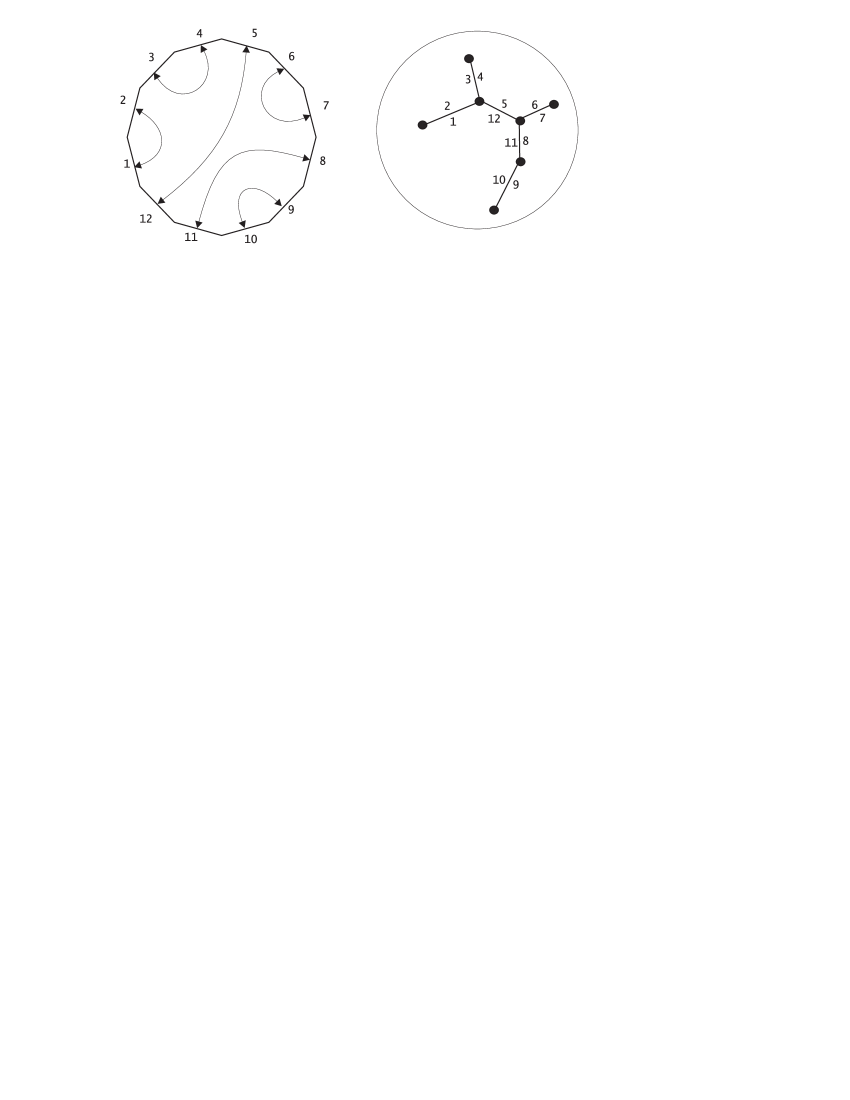
Figure 4: A map on the sphere

The number of such noncrossing pairings is the Catalan number

$$\left|\operatorname{Map}_{0}(2k)\right|=C_{k}=\frac{1}{k+1}\binom{2k}{k}\,.$$

The Stirling formula gives

$$\operatorname{map}_{0}(\xi)=\frac{1}{\sqrt{\pi}}\left(\frac{\xi}{2}\right)^{-3/2}\,.$$ (2.13)

We have

$$\left\langle{\widehat{y}(\xi)}\right\rangle=\int_{\mathbb{R}^{1}}e^{\xi y}\,\rho(y)\,dy=\frac{1}{2}\sum_{g=0}^{\infty}\operatorname{map}_{g}(\xi)\,,$$ (2.14)

where

$$\rho(y)=K(y,y)$$

is the 1-point correlation functions for the $y_{i}$’s, that is, $\rho(y)\,dy$ is the probability to find one of the $y_{i}$’s in the interval $[y,y+dy]$. A formula for this $1$-point function is given in (2.10).

Assuming that we already know that the degree of $\operatorname{map}_{g}(\xi)$ is positive for $g>0$, we conclude that

$$\int e^{\xi y}\,\rho(y)\,dy\sim\sqrt{\frac{2}{\pi}}\,\frac{1}{\xi^{3/2}}\,,\quad\xi\to+0\,.$$ (2.15)

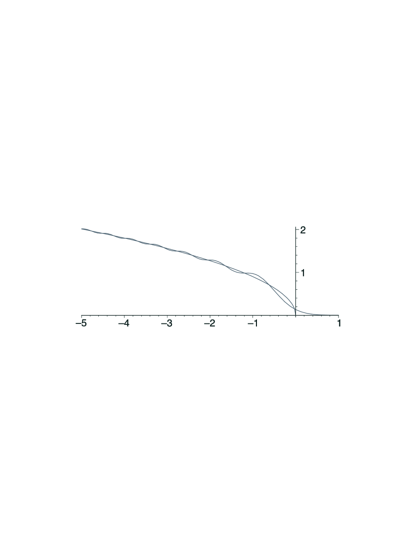
Figure 5: Density $\rho$ of the $y_{i}$’s versus $2^{3/2}\sqrt{-x}/\pi$

This asymptotics reflects the $y\to-\infty$ asymptotics of $\rho(y)$ which is known to be, see Figure 5,

$$\rho(y)\sim\frac{2^{3/2}}{\pi}\sqrt{-y}\,,\quad y\to-\infty\,.$$

This is in agreement with (2.15).

2.2.2

Below we will need the following elementary lemma about Catalan numbers

Lemma 1

We have

$$C_{k}<\frac{1}{\sqrt{\pi}}\frac{2^{2k}}{k^{3/2}}\,,\quad k=1,2,\dots\,.$$

That is, Catalan numbers $C_{k}$ are less than their $k\to\infty$ asymptotics.

To verify this, set

$$\widetilde{C}_{k}=C_{k}\,\frac{k^{3/2}}{2^{2k}}\to\frac{1}{\sqrt{\pi}}\,,\quad k\to\infty\,.$$

We claim that the sequence $\widetilde{C}_{k}$ is strictly increasing, which is equivalent to

$$\frac{\widetilde{C}_{k+1}}{\widetilde{C}_{k}}=\frac{(k+1)^{3/2}}{k^{3/2}}\,\frac{k+\frac{1}{2}}{k+2}>1$$

for $k\geq 1$. Indeed this ratio tends to $1$ as $k\to\infty$ and its derivative in $k$ is negative:

$$\left(\frac{(k+1)^{3/2}}{k^{3/2}}\,\frac{k+\frac{1}{2}}{k+1}\right)^{\prime}=-\frac{3}{4}\,\frac{(k+1)^{1/2}}{k^{5/2}}\,\frac{3k+2}{(k+2)^{2}}\,.$$

Thus, $\widetilde{C}_{k}$ is strictly less than the limit $\pi^{-1/2}$ as was to be shown.

2.2.3

Another special example to consider is the case $s=2$, $g=0$. These are the two cases not covered by the general construction explained in the next subsection.

2.3 Counting maps

2.3.1 The contraction $\Phi$

We will now count the the maps in all cases except $s=1,2$, $g=0$. In fact, in order to establish connection with random permutations it is not necessary to actually compute the asymptotics explicitly. It suffices to establish just the general pattern of the combinatorial enumeration which occurs. Nonetheless, we do the computations because in the end we will be rewarded with a connection to the moduli spaces of curves.

In order to count the maps, we will construct a function $\Phi$ from the set of maps to a simpler set such that the level sets of $\Phi$ are easy to understand. This is like computing the volume by integrating first along the fibers of a projection and then over the base. More concretely, the target set of our function $\Phi$ will be set of pairs

$$\Phi:\operatorname{Map}_{g}(k_{1},\dots,k_{s})\to\{(\Gamma,\ell)\}\,,\quad\Gamma\in\Gamma^{\geq 3}_{g,s}\,,$$

where $\Gamma^{\geq 3}_{g,s}$ denotes ribbon graphs of genus $g$ with $s$ marked cells and vertices of valence $\geq 3$, and $\ell$ is a metric on the boundary $\partial\Gamma$ of $\Gamma$.

2.3.2

Recall that, by definition, a ribbon graph is the following object. It is a union of vertices (which are small disks or polygons; we shall paint them grey in the figures) which are connected by ribbons (edges). The boundary $\partial\Gamma$ of a ribbon graph $\Gamma$ is an ordinary graph whose edges are the borders of the ribbons. Let $s$ be the number of connected components of $\partial\Gamma$. Filling each component of $\partial\Gamma$ with a disk produces a closed surface. The genus of $\Gamma$ is, by definition, the genus of that surface. The components of $\partial\Gamma$ (or the disks filling them) are called the cells of $\Gamma$. We shall consider ribbon graphs with $s$ cells and the cells will be marked by the numbers $\{1,2,\dots,s\}$.

2.3.3

Given a map on a surface $\mathsf{S}$, consider the the graph on $\mathsf{S}$ formed by vertices and edges of the original polygons. A small neighborhood of this graph is a ribbon graph. The numbering of the cells comes from the numbering of the polygons of the map.

For example, consider the map on the torus which is drawn in Figure 6.

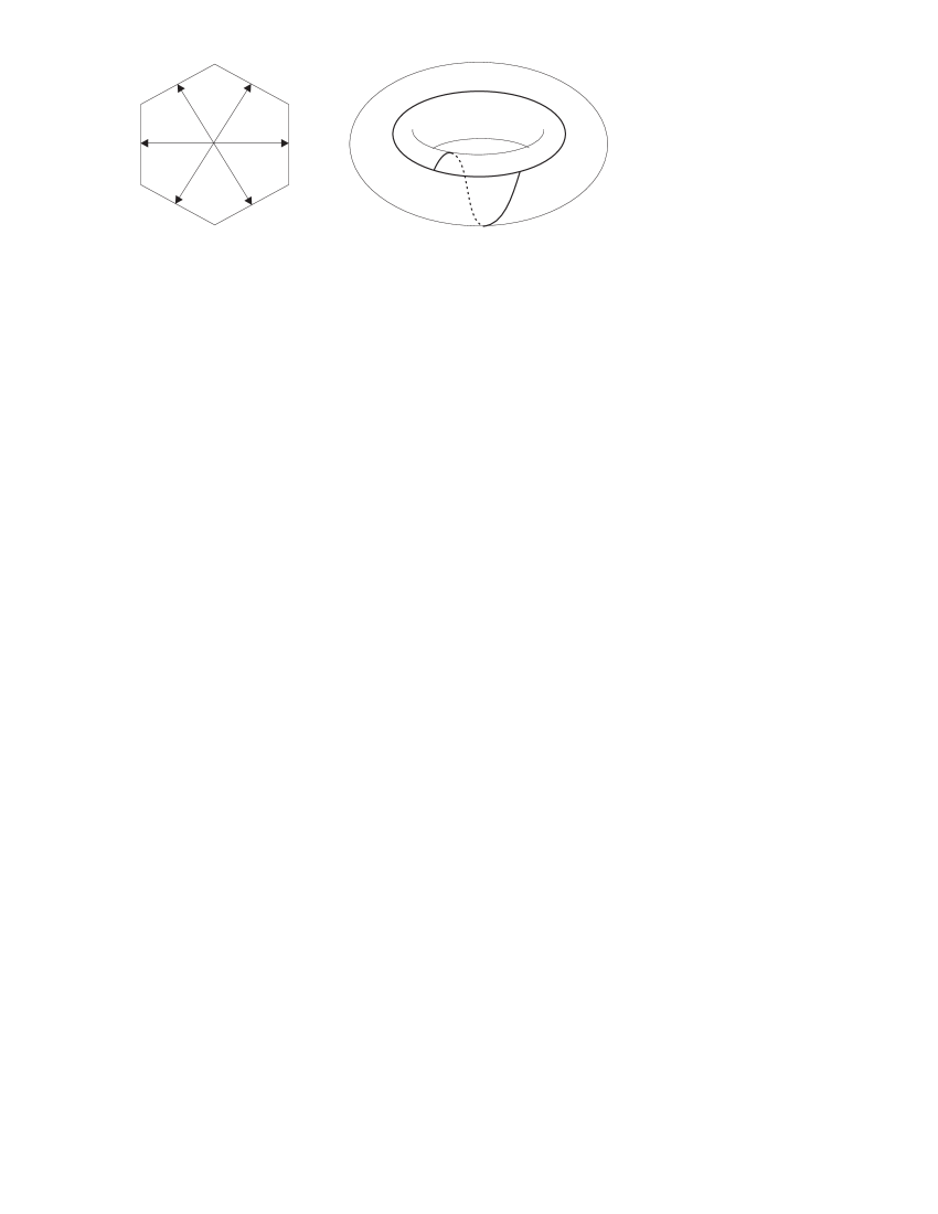
Figure 6: A map on the torus

The corresponding ribbon graph is displayed in Figure 7. There is only one cell in this example.

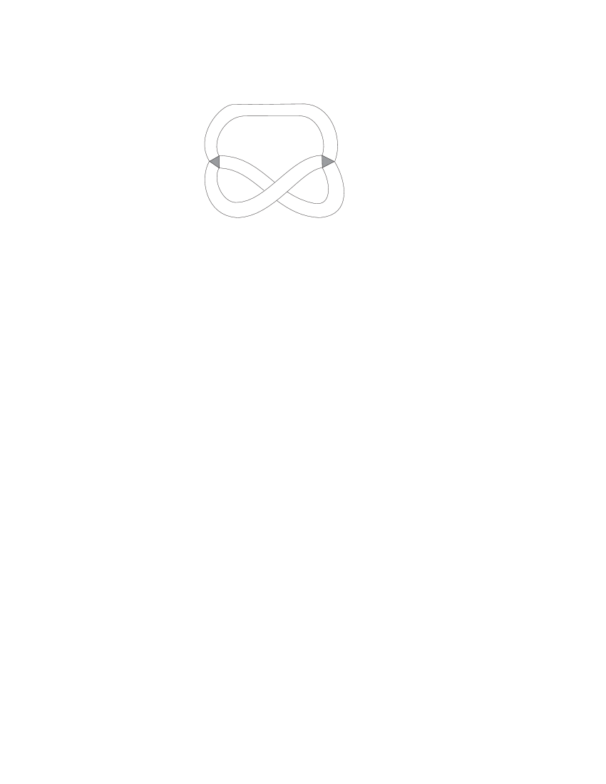
Figure 7: The corresponding ribbon graph

We equip the boundary of this graph with the metric $\ell$ in which all edges have unit length. Thus, we associated to any map a pair $(\Gamma_{0},\ell)$, where $\Gamma_{0}$ is ribbon graph of genus $g$ with $s$ marked cells and $\ell$ is a metric on $\partial\Gamma_{0}$. This pair is the first step in the construction of $\Phi$.

2.3.4

The second step on the construction of $\Phi$ is the elimination of all vertices of valence $\leq 2$ from $\Gamma_{0}$. This goes as follows.

First, we collapse the univalent vertices as in Figure 8. The numbers in that picture illustrate what we do with the metric $\ell$. Namely, we increase the length of the adjacent (with respect to the orientation) part of the boundary by the total perimeter of the disappearing edge. Note that this operation preserves perimeters of cells.

Figure 8: Collapsing of univalent vertices

After that, the vertices of valence 2 are eliminated as in Figure 9. Again, the perimeters of cell are preserved by this operation.

Figure 9: Elimination of 2-valent vertices

In the end, we get a ribbon graph $\Gamma\in\Gamma^{\geq 3}_{g,s}$, provided we are not in the exceptional cases $g=0$, $s=1,2$ in which we get a point and circle, respectively. We also get a metric $\ell$ on $\partial\Gamma$. By definition, this pair $(\Gamma,\ell)$ is where $\Psi$ takes our original map.

2.3.5

Note that, by construction, the perimeters of the cells of $\Gamma$ are equal to $k_{1},k_{2},\dots,k_{s}$. Also, the computation of the Euler characteristic gives

$$\sum_{v\in v(\Gamma)}(\operatorname{val}(v)-2)=4g-4+2s\,,$$ (2.16)

where $v(\Gamma)$ is the set of vertices of $\Gamma$.

All this is, of course, very similar to the stratification of the moduli space of curves of genus $g$ with $s$ marked points by means of Strebel differentials, see e. g. [19].

2.4 The level sets of the contraction $\Phi$

2.4.1

We now want to compute how many maps $\Phi$ takes to a given pair $(\Gamma,\ell)$. First, look at a single edge of $\Gamma$ let $p$ and $q$ the lengths of its two boundaries in metric $\ell$. We want to compute how many different configurations produce this data after the elimination of vertices of valence $\leq 2$.

This means that we must compute the number of ribbon graphs of the form shown in Figure 10

Figure 10: A ribbon graph which collapses to an edge

with the length of the upper boundary and lower boundary being $p$ and $q$, respectively. The trees in Figure 10 stand for (possibly empty) ribbon graphs which disappear after collapsing all univalent vertices. It implies that they are trees in the usual sense of graph theory.

Remark that a tree is not allowed at one of the ends of both upper and lower boundary. This corresponds to our convention (see Figure 8) on where we transfer the length of a collapsing edge. However, a simple shift as in Figure 11

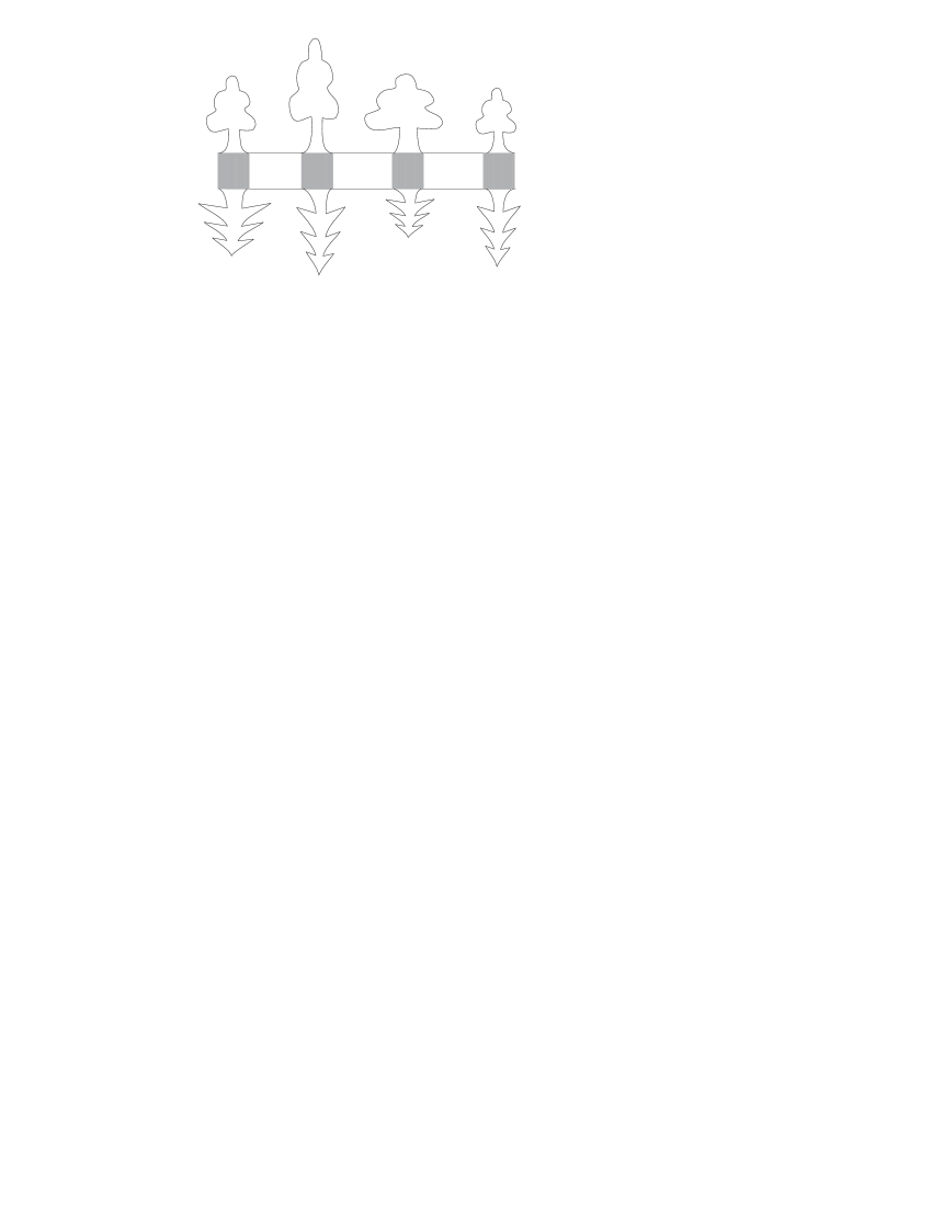
Figure 11: A shift of Figure 10

which reduces the length of both boundaries by 1, takes care of this inconvenience. Now it clear that to obtain a ribbon graph like in Figure 11 one just takes any map from $\operatorname{Map}_{0}(p+q-2)$ and calls the first $(p-1)$ sides the upper boundary, and rest — the lower boundary. Therefore, we get a Catalan number provided $p+q$ is even (and $0$ otherwise). This means that there are

$$\sim\frac{1}{\sqrt{2\pi}}\frac{2^{p+q}}{(p+q)^{3/2}}\,,\quad p+q\to\infty\,,$$ (2.17)

ribbon graphs which collapse to an edge with length of the upper and lower boundary equal to $p$ and $q$, respectively. Moreover, by Lemma 1 the actual number of such maps is always less than (2.17).

2.4.2

Now consider all edges of $\Gamma$. It is clear that we can apply the above construction to every edge of $\Gamma$ independently and the only situation in which we get identical maps is when the maps differ by an automorphism of $\Gamma$. Here by an automorphism we mean automorphisms of the whole structure of a ribbon graph with marked cells; in particular, the automorphisms must preserve cells.

Also recall that we consider maps with marked vertices. Since marks can be chosen arbitrarily on the boundary of each cell, we have

$$\left|\Phi^{-1}((\Gamma,\ell))\right|\sim\frac{\prod k_{i}}{|\operatorname{Aut}(\Gamma)|}\,\frac{2^{|k|}}{(2\pi)^{|e(\Gamma)|/2}}\,\prod_{e\in e(\Gamma)}(\ell_{1,e}+\ell_{2,e})^{-3/2}\,.$$ (2.18)

where the $k_{i}$ are the perimeters of the cells of $\Gamma$ and their product is the number of choices for the marked vertices. Here $\ell_{1,e}$ and $\ell_{2,e}$ are the lengths of the two sides of the edge $e\in e(\Gamma)$ in the metric $\ell$.

Again, by Lemma 1 the right-hand side of (2.18) is both asymptotics and an estimate from above for the left-hand side.

2.5 The asymptotics

2.5.1

Now we want to sum (2.18) over the metrics $\ell$. This means summation over points in $\mathbb{R}^{2|e(\Gamma)|}$ satisfying the following properties

• the values of $\ell$ are integers and for any $e\in e(\Gamma)$ the sum $\ell_{1,e}+\ell_{2,e}$ is an even integer,

• the lengths of the edges are nonnegative and the perimeters of the $s$ cells are equal to $k_{1},\dots,k_{s}$, respectively.

It is clear that the first condition defines a sublattice $\Lambda$ of index $\left|e(\Gamma)\right|$ in $\mathbb{Z}^{2|e(\Gamma)|}$. The second condition defines a convex polytope which we denote by $\operatorname{Met}_{\Gamma}(k)$. The dimension of this polytope is

$$\dim\operatorname{Met}_{\Gamma}(k)=2|e(\Gamma)|-s\,.$$ (2.19)

By definition, let $\operatorname{Map}_{g,\Gamma}(k)$ denote those maps in $\operatorname{Map}_{g}(k)$ which correspond to a given graph $\Gamma$ under $\Phi$. It follows that

$$\left|\operatorname{Map}_{g,\Gamma}(k)\right|=\sum_{\ell\in\operatorname{Met}_{\Gamma}(k)\cap\Lambda}\left|\Phi^{-1}((\Gamma,\ell))\right|\,.$$ (2.20)

This is a summation over lattice points in the polytope $\operatorname{Met}_{\Gamma}(k)$. As the $k_{i}$’s go to infinity, the sum (2.20) after proper scaling will produce an integral.

More precisely, note that, aside from the factor $2^{|k|}$, the right-hand side of (2.18) is homogeneous in $k$ and $\ell$ of degree $s-\frac{3}{2}|e(\Gamma)|$. Therefore, if the $k_{i}$’s go to infinity in such a way that

$$k_{i}\sim t\cdot\xi_{i}\,,\quad t\to\infty\,,$$

the sum (2.20) becomes the following integral

$$\left|\operatorname{Map}_{g,\Gamma}(k)\right|\sim\\ \frac{t^{|e(\Gamma)|/2}}{|\operatorname{Aut}(\Gamma)|}\frac{2^{|k|-3|e(\Gamma)|/2+1}}{\pi^{|e(\Gamma)|/2}}\prod_{1}^{s}\xi_{i}\int_{\operatorname{Met}_{\Gamma}(\xi)}d\ell\,\prod_{e\in e(\Gamma)}(\ell_{1,e}+\ell_{2,e})^{-3/2}\,,$$ (2.21)

where the normalization of Lebesgue measure on the polytope $\operatorname{Met}_{\Gamma}(\xi)$ is explained in the next subsection.

The validity of the replacing sums by integrals is justified by the dominated convergence theorem, Lemma 1, and the convergence of the following integral

$$\iint_{\begin{subarray}{c}\!\!x,y\geq 0\\ \!\!x+y\leq c\end{subarray}}\,\,\frac{dx\,dy}{(x+y)^{3/2}}=\int_{0}^{c}\frac{du}{\sqrt{u}}\,,\quad u=x+y\,.$$

2.5.2

The Lebesgue measure the right-hand side of (2.21) is normalized as follows.

Let $A$ be an open subset of $\operatorname{Met}_{\Gamma}(\xi)$. The polytope $\operatorname{Met}_{\Gamma}(\xi)$ is the polytope $\operatorname{Met}_{\Gamma}(k)$ scaled by a factor of $t^{-1}$ and so $tA\subset\operatorname{Met}_{\Gamma}(k)$. The number of integer points, that is, the points of the standard lattice $\mathbb{Z}^{2|e(\Gamma)|}$ in $\operatorname{Met}_{\Gamma}(k)$ grows like $t^{\dim\operatorname{Met}_{\Gamma}(k)}$, where the dimension is given by (2.19). We normalize the Lebesgue measure on $\operatorname{Met}_{\Gamma}(\xi)$ by

$$\int_{A}d\ell=\lim_{t\to\infty}t^{s-2|e(\Gamma)|}\,\left|tA\cap\mathbb{Z}^{2|e(\Gamma)|}\right|\,.$$

The summation in (2.20) is not over all integer points but over points in the sublattice $\Lambda\subset\mathbb{Z}^{2|e(\Gamma)|}$ of index $2^{|e(\Gamma)|}$. Observe that when we intersect both lattices with the affine span of $\operatorname{Met}_{\Gamma}(k)$ the index drops to $2^{|e(\Gamma)|-1}$ because one of the parity conditions becomes redundant once the total perimeter is fixed. Hence

$$\lim_{t\to\infty}t^{s-2|e(\Gamma)|}\,\left|tA\cap\Lambda\right|=2^{1-|e(\Gamma)|}\,\int_{A}d\ell\,.$$

This is reflected in the fact that the exponent of 2 in (2.18) and (2.21) differ by $|e(\Gamma)|-1$.

2.5.3

Consider the sum

$$\left|\operatorname{Map}_{g}(k_{1},\dots,k_{s})\right|=\sum_{\Gamma\in\Gamma^{\geq 3}_{g,s}}\left|\operatorname{Map}_{g,\Gamma}(k)\right|\,.$$

Observe, that some of the summands are asymptotically negligible. Indeed, it is clear from (2.21) that the asymptotics is determined by those $\Gamma$ that have the maximal number of edges. Equivalently, by invariance of the Euler characteristic, they must have the maximal number of vertices. From (2.16) it follows that this happens if and only if all vertices of $\Gamma$ are trivalent.

Denote by $\Gamma^{3}_{g,s}$ the subset of $\Gamma^{\geq 3}_{g,s}$ formed by trivalent graphs. Remark that every $\Gamma\in\Gamma^{3}_{g,s}$ has $6g-6+3s$ edges.

We have established the following result

Proposition 1

$$\frac{\operatorname{map}_{g}(\xi_{1},\dots,\xi_{s})}{\xi_{1}\cdots\xi_{s}}=\\ \frac{2}{(8\pi)^{3g-3+3s/2}}\sum_{\Gamma\in\Gamma^{3}_{g,s}}\frac{1}{|\operatorname{Aut}(\Gamma)|}\int_{\operatorname{Met}_{\Gamma}(\xi)}d\ell\,\prod_{e\in e(\Gamma)}(\ell_{1,e}+\ell_{2,e})^{-3/2}\,,$$ (2.22)

where $\ell_{1,e}$ and $\ell_{2,e}$ are the lengths of the two sides of the edge $e\in e(\Gamma)$ in the metric $\ell$.

2.5.4

Using the integral

$$\frac{1}{\sqrt{\pi}}\int_{0}^{\infty}\int_{0}^{\infty}\frac{e^{-ax-by}}{(x+y)^{3/2}}\,dx\,dy=\frac{2}{\sqrt{a}+\sqrt{b}}\,,\quad\Re a,\Re b>0\,.$$ (2.23)

we can compute the Laplace transform of (2.22) in a compact form. Take some $z_{1},\dots,z_{s}$ such that $\Re z_{i}>0$.

We have

$$\int_{\mathbb{R}_{\geq 0}^{s}}e^{-(z,\xi)}\,\operatorname{map}_{g}(\xi)\,\frac{d\xi}{\xi}=\sum_{\Gamma}\int_{\mathbb{R}_{\geq 0}^{s}}{d\xi}\int_{\operatorname{Met}_{\Gamma}(\xi)}d\ell\,(\dots)$$

and each summand in the right-hand side is an integral over all possible metrics $\ell$ on $\partial\Gamma$, that is, just an integral over $\mathbb{R}_{\geq 0}^{2|e(\Gamma)|}$. It factors into a product of integrals of the form (2.23) over the edges of $\Gamma$.

Thus, we obtain the following

Theorem 3

The Laplace transform of the function $\operatorname{map}_{g}(\xi)$ equals

$$\int_{\mathbb{R}_{\geq 0}^{s}}e^{-(z,\xi)}\,\operatorname{map}_{g}(\xi)\,\frac{d\xi}{\xi}=2\sum_{\Gamma\in\Gamma^{3}_{g,s}}\frac{1}{|\operatorname{Aut}(\Gamma)|}\prod_{e\in e(\Gamma)}\frac{2^{-1/2}}{\sqrt{z_{1,e}}+\sqrt{z_{2,e}}}\,.$$ (2.24)

Here $\Gamma^{3}_{g,s}$ is the set of 3-valent ribbon graphs of genus $g$ with $s$ cells numbered by $1,2,\dots,s$, $e(\Gamma)$ is the set of edges of $\Gamma$, and $z_{1,e}$ and $z_{2,e}$ are the two $z_{i}$’s which correspond to the two sides of an edge $e\in e(\Gamma)$.

2.5.5

The right-hand side is, up to the presence of square roots and difference in the exponent of $2$, identical to the right-hand side of the main formula in [19]. This relation is not accidental. In fact, our counting problem is very directly related to Kontsevich’s combinatorial description of the intersection numbers on the moduli spaces. This connection is as follows.

Consider the following function

$$\widehat{M}_{g}(z_{1},\dots,z_{2})=\sum_{k}e^{-(z,k)}\,\frac{\operatorname{Map}_{g}(k_{1},\dots,k_{s})}{2^{|k|}\prod k_{i}}\,.$$ (2.25)

By definition of $\operatorname{map}_{g}$, we have

$$N^{-3g+3-3s/2}\,\widehat{M}_{g}\left(\frac{z}{N}\right)\to\frac{1}{2}\int_{\mathbb{R}_{\geq 0}^{s}}e^{-(z,\xi)}\,\operatorname{map}_{g}(\xi)\,\frac{d\xi}{\xi}\,,$$

where the factor $\frac{1}{2}$ comes from the fact that the summation is (2.25) is in fact over all $k$ such that $|k|$ is even which is an index $2$ sublattice in $\mathbb{Z}^{s}$.

It is clear from our discussion that (2.25) is a sum over ribbon graphs with vertices of valence $\geq 3$. The contribution of each graph $\Gamma$ is the reciprocal of $|\operatorname{Aut}(\Gamma)|$ times the product of the following contributions of the edges $e$ of $\Gamma$. Let $z$ and $w$ be the $z_{i}$’s corresponding to the two sides of $w$, then the contribution $C$ of the edge $e$ is

$$C(z,w)=\sum_{p,q}e^{-zp-qw}\,2^{-p-q}\,c_{p,q}\,,$$

where $c_{p,q}$ is the number of ribbon graphs like the one shown in Figure 10 with length of the upper and lower boundary being equal to $p$ and $q$ respectively.

Let us forget for a moment that $c_{p,q}$ is just a Catalan number. Let us think of the Figure 10 as of an alley with trees growing on both sides. The total perimeter of trees on the two sides is $p$ and $q$. Let $r$ be the length of the alley itself, for example, $r=4$ in Figure 10. Let $t_{p,r}$ denote the number of ways to plant trees of total perimeter $p$ along an alley of length $r$ so that there is no tree at the very end of the alley. Clearly

$$C(z,w)=\sum_{r}\left(\sum_{p}e^{-zp}\,2^{-p}\,t_{p,r}\right)\,\left(\sum_{p}e^{-zq}\,2^{-q}\,t_{q,r}\right)\,.$$

It is well known that $t_{p,r}$ also count all trajectories of a random walk which starting from zero first reach $r$ in $p$ steps, see Figure 12.

Figure 12: Bijection between planting trees and random walk

The bijection is very simple: we start a new branch whenever we go down and finish an existing branch or go to the next tree whenever we go up.

Now consider the asymptotics of $C(z/N,w/N)$ as $N\to\infty$. If $p$ is scaled by $N$ and $r$ by $\sqrt{N}$ then $2^{-p}\,t_{p,r}$ becomes the probability for the standard Brownian motion to first reach $r$ in time $p$, which is well known to have the density, see e.g. Section V.3.2 in [34],

$$\frac{r}{\sqrt{2\pi p^{3}}}\,e^{-r^{2}/2p}\,dp$$

with the Laplace transform

$$\int_{0}^{\infty}e^{-zp}\,\frac{r}{\sqrt{2\pi p^{3}}}\,e^{-r^{2}/2p}\,dp=e^{-r\sqrt{2z}}\,.$$ (2.26)

Hence

$$N^{-1/2}\,C(z/N,w/N)\to\int_{0}^{\infty}e^{-r\left(\sqrt{2z}+\sqrt{2w}\right)}\,dr=\frac{2^{-1/2}}{\sqrt{z}+\sqrt{w}}\,.$$

Kontsevich’s combinatorial model for intersection numbers on the moduli spaces of curves leads to counting alleys with no trees at all, in which case the length $r$ of the alley is simultaneously the length of its both boundaries. In our case, things are dressed up with trees but as (2.26) shows this amounts to just replacing Laplace transform variables by their square roots.

2.6 Example: 1-cell maps of genus $\geq 1$

2.6.1

Consider the case $s=1$, $g=1$. In this case, the set $\Gamma^{3}_{g,s}$ consists of one element which is displayed in Figures 6 and 7. The automorphism group of this graph is the cyclic group of order 6 which is clearly seen in the left half of Figure 6. Also, there is only one $z$ which corresponds to both sides of every edge. Therefore,

$$\int_{0}^{\infty}e^{-z\xi}\,\operatorname{map}_{1}(\xi)\,\frac{d\xi}{\xi}=\frac{1}{6}\frac{1}{2^{7/2}}\frac{1}{z^{3/2}}\,,$$

which implies that

$$\operatorname{map}_{1}(\xi)=\frac{1}{12\sqrt{\pi}}\left(\frac{\xi}{2}\right)^{3/2}\,.$$

2.6.2

In general, for $s=1$ and any $g$ we have

$$\operatorname{map}_{g}(\xi)\propto\xi^{3g-3/2}\,.$$

The constant can be fixed using the following exact result of Harer and Don Zagier [15]

$$\left|\operatorname{Map}_{g}(2k)\right|=\frac{(2k)!}{(k+1)!\,(k-2g)!}\,\left[x^{2g}\right]\,\left(\frac{x/2}{\tanh x/2}\right)^{k+1}\,,$$ (2.27)

where $\left[x^{2g}\right]$ stands for the coefficient of $x^{2g}$. We have

$$\frac{x/2}{\tanh x/2}=1+\frac{x^{2}}{12}+\dots\,,$$

which implies that

$$\operatorname{map}_{g}(\xi)=\frac{1}{\sqrt{\pi}}\frac{1}{12^{g}g!}\left(\frac{\xi}{2}\right)^{3g-3/2}\,.$$

2.6.3

As an exercise, let us check that this is in agreement with (2.14) and (2.10). In other words, we have to check the identity

$$\int_{-\infty}^{\infty}e^{\xi x}\,K(x,x)\,dt=\frac{1}{2\sqrt{\pi}}\,\frac{e^{\xi^{3}/12}}{\xi^{3/2}}\,.$$ (2.28)

where $K(x,x)$ is defined by (2.10).

From the differential equation for the Airy function one obtains

$$\frac{d^{3}}{dx^{3}}K(x,x)-4x\frac{d}{dx}K(x,x)+2K(x,x)=0\,.$$

Therefore, its Laplace transform of $K$ must satisfy a first order ODE which the right-hand side of (2.28) indeed satisfies. This proves the equality (2.28) up to a constant factor. The factor is fixed by the asymptotics $\xi\to+0$ which was considered in Section 2.2.

2.6.4

As another application of the exact formula (2.27), let us prove that taking term-wise limit in

$$\frac{1}{2^{k}n^{k/2}}\left\langle{\operatorname{tr}H^{k}}\right\rangle=\sum_{g\geq 0}n^{1-2g}\,\frac{|\operatorname{Map}_{g}(k)|}{2^{k}}$$ (2.29)

is justified. We have

$$\frac{x}{\tanh x}=1-2\sum_{g=0}^{\infty}(-1)^{g}\,\zeta(2g)\,\frac{x^{2g}}{\pi^{2g}}$$

and since $\zeta(2g)<\zeta(2)=\pi^{2}/6$ for $g>1$, the coefficient of $x^{2g}$ in the above series is less or equal than $3^{-g}$ in absolute value for any $g$. Therefore, the the coefficients of $(1-x^{2}/12)^{-k-1}$ dominate the coefficients of $\left(\frac{x/2}{\tanh x/2}\right)^{k+1}$ which implies that

$$\left|\operatorname{Map}_{g}(2k)\right|\leq\frac{(2k)!}{(k+1)!\,(k-2g)!}\,\binom{k+g}{g}\,12^{-g}\leq\frac{1}{\sqrt{\pi}}\,\frac{2^{2k}\,k^{3g-3/2}}{g!}\,,$$ (2.30)

where in the second inequality we used Lemma 1 and the inequality $2g\leq k$ which implies that

$$\binom{k+g}{g}\leq\frac{(\frac{3}{2}\,k)^{g}}{g!}\,.$$

The inequality (2.30) justifies taking term-wise asymptotics in (2.29) provided $k\propto n^{2/3}$ and also yields that

$$\frac{1}{2^{k}n^{k/2}}\left\langle{\operatorname{tr}H^{k}}\right\rangle\leq\frac{2^{3/2}}{\sqrt{\pi}}\,\frac{e^{\xi^{3}/8}}{\xi^{3/2}}\,,\quad\xi=k\,n^{-2/3}\,.$$ (2.31)

Using (2.4) and (2.6) we obtain

$$\frac{1}{2^{|k|}n^{|k|/2}}\left\langle{\prod_{j=1}^{s}\operatorname{tr}H^{k_{i}}}\right\rangle\leq\textup{some function of $\xi_{i}=k_{i}\,n^{-2/3}$}\,.$$ (2.32)

This estimate justifies taking the term-wise limit in (2.5).

3 Random permutations and coverings

3.1 Jucys-Murphy elements

3.1.1 Definition

Consider the following elements $X_{1},X_{2},\dots$ of the group algebra of the symmetric group $S(n)$

$$X_{1} =(12)+ (13)+ (14)+(15)+\dots\,,$$

$$X_{2} = (23)+ (24)+(25)+\dots\,,$$

$$X_{3} = (34)+(35)+\dots\,,$$

and so on. These elements are called the Jucys-Murphy elements, or JM elements for short. For a modern introduction to their properties the reader is referred to [32]. See also for example [5, 25, 28, 29] for various applications of these elements.

These elements are truly remarkable. Most importantly, they commute and generate a maximal commutative subalgebra in the group algebra of $S(n)$ which is exactly the algebra of elements acting diagonally the Young basis of irreducible representations of $S(n)$. Since this fact is central to what follows, we will review it briefly.

3.1.2 Eigenvalues

Let $\lambda$ be a partition of $n$ and consider the corresponding representation of the $S(n)$. The eigenvalues of the self-adjoint element $X_{1}$ in the representation $\lambda$ correspond to the corners of the diagram $\lambda$ as follows.

Let a square $(i,\lambda_{i})\in\lambda$ be a corner of the diagram $\lambda$ which means that $\lambda_{i}>\lambda_{i+1}$. Then $\lambda_{i}-i$ is an eigenvalue of $X_{1}$. Recall that the difference between the column number and the row number of a square $\square\in\lambda$ is called the content of $\square$. That is, the eigenvalues of $X_{1}$ are precisely the contents of the corner squares of $\lambda$. If one takes Figure 1 and adds the eigenvalues of the $X_{1}$ one obtains Figure 13.

Figure 13: Eigenvalues of the $X_{1}$

3.1.3 Eigenspaces

Now consider the eigenspaces of $X_{1}$. The subgroup

$$S(n)\supset S_{1}(n)\cong S(n-1)\,,$$

of permutations which fix $1\in\{1,\dots,n\}$ commutes with $X_{1}$ and thus preserves the eigenspaces of $X_{1}$.

In fact, the $\lambda_{i}-i$ eigenspace of $X_{1}$ is an irreducible module over $S_{1}(n)\cong S(n-1)$. Moreover, as an $S(n-1)$-module it corresponds to the diagram

$$\lambda-\square_{i}=(\lambda_{1},\lambda_{2},\dots,\lambda_{i}-1,\dots)$$

obtained from $\lambda$ by removing the square $\square_{i}=(i,\lambda_{i})$. In particular, the multiplicity of the eigenvalue $\lambda_{i}-i$ equals the dimension $\dim(\lambda-\square_{i})$.

3.1.4 Action in the regular representation

Consider the action of $X_{1}$ in the regular representation, that is, the representation of $S(n)$ by multiplication on the group algebra $\mathbb{C}S(n)$. Since the multiplicity of every representation $\lambda$ in $\mathbb{C}S(n)$ equals its dimension we find that

$$\frac{1}{n!}\,\operatorname{tr}X_{1}^{k} =\frac{1}{n!}\,\sum_{|\lambda|=n}\dim\lambda\sum_{i}\dim(\lambda-\square_{i})\,(\lambda_{i}-i)^{k}$$

$$=\sum_{|\lambda|=n}\mathfrak{P}_{n}(\lambda)\sum_{i}\delta_{i}(\lambda)\,(\lambda_{i}-i)^{k}\,,$$ (3.1)

where the trace is taken in the regular representation, we agree that $\dim(\lambda-\square_{i})=0$ if the square $\square_{i}$ is not a corner of $\lambda$, and we set, by definition,

$$\delta_{i}(\lambda)=\frac{\dim(\lambda-\square_{i})}{\dim\lambda}\,.$$ (3.2)

The purpose of introducing the ratio (3.2) is that it is much simpler than both its numerator and denominator. Indeed, from the formula

$$\dim\lambda=|\lambda|!\,\left.\prod_{i<j\leq\ell(\lambda)}(\lambda_{i}-\lambda_{j}+j-i)\right/\prod_{i\leq\ell(\lambda)}(\lambda_{i}+\ell(\lambda)-i)\,!\,,$$

where $\ell(\lambda)$ is the length of the partition $\lambda$, that is, the number of nonzero parts in $\lambda$, it follows that

$$\delta_{i}(\lambda)=\frac{\lambda_{i}+\ell(\lambda)-i}{|\lambda|}\,\prod_{j\leq\ell(\lambda),j\neq i}\left(1-\frac{1}{\lambda_{i}-\lambda_{j}+j-i}\right)\,.$$ (3.3)

In the next subsection we will investigate the behavior of $\delta_{i}(\lambda)$ for a $\mathfrak{P}_{n}$-typical $\lambda$ as $n\to\infty$.

3.2 Growth and decay of partitions

3.2.1 Rates of growth and decay

It is clear that

$$\dim\lambda=\sum_{i}\dim(\lambda-\square_{i})\,,$$ (3.4)

and hence $\delta_{i}(\lambda)$ is naturally a probability measure on the corners of the diagram $\lambda$, that is,

$$\sum_{i}\delta_{i}(\lambda)=1\,,\quad\delta_{i}(\lambda)\geq 0\,.$$

One can construct a Markov process on the set of all partitions with transition probabilities

$$\operatorname{Prob}\left\{\lambda\mapsto\lambda-\square_{i}\right\}=\delta_{i}(\lambda)\,.$$

The representation-theoretic meaning of this decay process is the branching of representations of symmetric group under restriction onto a smaller symmetric group.

Conversely, induction of representations gives a natural Markov growth process for partitions with transition probabilities

$$\operatorname{Prob}\left\{\lambda\mapsto\lambda+\square_{i}\right\}=\delta^{*}_{i}(\lambda)\,,$$

where

$$\delta^{*}_{i}(\lambda)=\frac{1}{|\lambda|+1}\,\frac{\dim(\lambda+\square_{i})}{\dim\lambda}\,.$$

We recall that the induction rule for representations of symmetric groups implies that

$$\dim\lambda=\frac{1}{|\lambda|+1}\sum_{i}\dim(\lambda+\square_{i})\,,$$ (3.5)

and hence $\delta^{*}_{i}(\lambda)$ is indeed a probability measure on $i$ for any $\lambda$. Geometrically those $i$ for which $\delta^{*}_{i}(\lambda)\neq 0$ correspond to places where one can add a square to $\lambda$, that is, to inner corners of the diagram $\lambda$.

The probabilities $\delta^{*}_{i}(\lambda)$ and $\delta_{i}(\lambda)$ are usually called the transition and cotransition probabilities, see for example [21, 23]. We will call them the rates of growth and decay, respectively.

3.2.2 Asymptotics of growth/decay rates

The equations (3.4) and (3.5) lead to the following conclusion: the decay and growth processes take the Plancherel measure on partition of $n$ to the Plancherel measure on partitions of $n-1$ and $n+1$, respectively.

We are interested in the asymptotics of $\delta_{i}(\lambda)$ for fixed $i$ and $\lambda$ being a Plancherel typical partition of $n$, $n\to\infty$. First, let us obtain this asymptotics heuristically.

Recall that for a Plancherel typical partition $\lambda$ of $n$ we have $\lambda_{i}\sim 2\sqrt{n}$, $n\to\infty$. This means that after $k$ iterations of the decay process, the length of the $i$-row will be $\sim 2\sqrt{n-k}$. Hence, the probability $\delta_{i}(\lambda)$ to remove a square from the $i$-th row of $\lambda$ should be

$$\delta_{i}(\lambda)\approx\frac{2\sqrt{n}-2\sqrt{n-k}}{k}\approx\frac{1}{\sqrt{n}}\,,\quad n\to\infty\,.$$

Now let us give a rigorous derivation of this asymptotics

Proposition 2

With respect to the Plancherel measure $\mathfrak{P}_{n}$ on partitions $\lambda$ of $n$,

$$\sqrt{n}\,\delta_{i}(\lambda)\to 1\,,\quad n\to\infty\,,$$

in probability for any fixed $i=1,2,\dots$

Let us begin with $i=1$. First we show that

$$\mathfrak{P}_{n}\left(\left\{\lambda,\sqrt{n}\,\delta_{i}(\lambda)\leq 1+\varepsilon\right\}\right)\to 1\,,\quad n\to\infty$$ (3.6)

for any $i=1,2,\dots$ and any $\varepsilon>0$. Recall that $\lambda_{1}\sim 2\sqrt{n}$ and similarly $\ell(\lambda)\sim 2\sqrt{n}$ for a Plancherel typical $\lambda$. Hence,

$$\lambda_{1}+\ell(\lambda)\sim 4\sqrt{n}\,,$$

and from (3.3) we obtain

$$\delta_{1}(\lambda)\sim\frac{4}{\sqrt{n}}\,\prod_{1<j\leq\ell(\lambda)}\left(1-\frac{1}{\lambda_{1}-\lambda_{j}+j-1}\right)\,.$$ (3.7)

Note that each factor in the (3.7) is $<1$.

The existence of the limit shape $\Omega$ of a typical $\lambda$ implies that for any $[a,b]\subset[-2,2]$ the number of $\lambda_{i}$’s such that $\lambda_{i}-i\in\sqrt{n}\,[a,b]$ is asymptotic to

$$\frac{1}{\sqrt{n}}\,\left|\left\{i,a\leq\frac{\lambda_{i}-i}{\sqrt{n}}\leq b\right\}\right|\sim\frac{\Omega(a)-a}{2}-\frac{\Omega(b)-b}{2}\,,\quad n\to\infty\,.$$

The product over all such $i$ in (3.7) can be estimated from above by

$$\exp\left(-\frac{1}{2-b}\left(\frac{\Omega(a)-a}{2}-\frac{\Omega(b)-b}{2}\right)\right)\,.$$

Hence, for any $\varepsilon>0$ we have

$$\delta_{1}(\lambda)<\frac{4+\varepsilon}{\sqrt{n}}\,\exp\left(-\int_{-2}^{2}\frac{1}{2-x}\,\frac{1-\Omega^{\prime}(x)}{2}\,dx\right)\,,$$

for a Plancherel typical $\lambda$ as $n\to\infty$.

This integral can be evaluated explicitly and one finds that

$$\exp\left(-\int_{-2}^{2}\frac{1}{2-x}\,\frac{1-\Omega^{\prime}(x)}{2}\,dx\right)=\frac{1}{4}\,.$$

Indeed, since

$$\frac{1-\Omega^{\prime}(x)}{2}=\frac{1}{\pi}\,\arccos\left(\frac{x}{2}\right)$$

one has to show that

$$\int_{-1}^{1}\frac{\arccos x}{1-x}\,dx=2\pi\ln 2\,.$$ (3.8)

Changing variables and integrating by parts we obtain

$$\int_{-1}^{1}\frac{\arccos x}{1-x}\,dx=\int_{0}^{\pi}\frac{t\,\sin t}{1-\cos t}\,dt=\pi\ln 2-\int_{0}^{\pi}\ln(1-\cos t)\,dt\,.$$

Using the Fourier expansion

$$\ln(1-\cos t)=\ln((1-e^{it})(1-e^{-it})/2)=-\ln 2-2\sum_{k=1}^{\infty}\frac{\cos kt}{k}$$

we obtain

$$\int_{0}^{\pi}\ln(1-\cos t)\,dt=-\pi\ln 2\,,$$

which establishes (3.8) and (3.6).

Observe that, by definition of $\delta^{*}_{1}(\lambda)$, we have

$$\delta^{*}_{1}(\lambda)=\frac{1}{n+1}\,\frac{1}{\delta_{1}(\lambda+\square_{1})}\,,\quad|\lambda|=n\,.$$

Since $\lambda+\square_{1}$ has the same limit shape $\Omega$, we obtain from (3.6) that

$$\mathfrak{P}_{n}\left(\left\{\lambda,\sqrt{n}\,\delta^{*}_{1}(\lambda)\geq 1-\varepsilon\right\}\right)\to 1\,,\quad n\to\infty$$ (3.9)

Now observe that

$$\sum_{|\lambda|=n}\delta^{*}_{1}(\lambda)\,\mathfrak{P}_{n}(\lambda)=\sum_{|\lambda|=n}\frac{\dim\lambda\,\dim(\lambda+\square_{1})}{(n+1)!}=\sum_{|\lambda|=n+1}\delta_{1}(\lambda)\,\mathfrak{P}_{n+1}(\lambda)\,.$$

This, together with (3.6) and (3.9) implies the existence of both limits

$$\sqrt{n}\,\delta_{1}(\lambda),\sqrt{n}\,\delta^{*}_{1}(\lambda)\to 1\,,\quad n\to\infty\,,$$

in probability.

Now consider the case $i=2$. First, show that $\lambda_{1}-\lambda_{2}\to\infty$ for typical $\lambda$ as $n\to\infty$. Indeed, the formula (3.7) can be rewritten as

$$\delta_{1}(\lambda)\sim\frac{4}{\sqrt{n}}\,\left(1-\frac{1}{\lambda_{1}-\lambda_{2}+1}\right)\,\prod_{2<j\leq\ell(\lambda)}\left(1-\frac{1}{\lambda_{1}-\lambda_{j}+j-1}\right)\,.$$ (3.10)

It is clear that our analysis of (3.7) really applies to the last factor in (3.10) which means that

$$\delta_{1}(\lambda)<\frac{1+\varepsilon}{\sqrt{n}}\left(1-\frac{1}{\lambda_{1}-\lambda_{2}+1}\right)$$

for typical $\lambda$. Since $\sqrt{n}\,\delta_{1}(\lambda)\to 1$ it follows that

$$\mathfrak{P}_{n}\left(\left\{\lambda,\lambda_{1}-\lambda_{2}>\operatorname{const}\right\}\right)\to 1\,,\quad n\to\infty$$ (3.11)

for any constant.

Therefore we can neglect $(\lambda_{1}-\lambda_{2}+1)^{-1}$ and write

$$\delta_{2}(\lambda)\sim\frac{4}{\sqrt{n}}\,\prod_{2<j\leq\ell(\lambda)}\left(1-\frac{1}{\lambda_{2}-\lambda_{j}+j-2}\right)\,.$$

We can apply to this formula exactly the same argument that we applied to (3.7) to show that

$$\sqrt{n}\,\delta_{2}(\lambda)\to 1\,,\quad n\to\infty\,,$$

in probability.

An identical argument proves that $\sqrt{n}\,\delta_{i}(\lambda)\to 1$ for any fixed $i$.

3.3 Plancherel averages and coverings

3.3.1

The formula (3.1) can be rewritten as

$$\frac{1}{2^{k}\,n^{(k-1)/2}\,n!}\,\operatorname{tr}X_{1}^{k}=\sum_{|\lambda|=n}\mathfrak{P}_{n}(\lambda)\sum_{i}\sqrt{n}\,\delta_{i}(\lambda)\,\left(\frac{\lambda_{i}-i}{2\sqrt{n}}\right)^{k}\,.$$ (3.12)

Consider the asymptotics of (3.12) as $n,k\to\infty$ in such a way that $kn^{-1/3}\to\xi$ for some fixed $\xi$.

The ratio $\dfrac{\lambda_{i}-i}{2\sqrt{n}}$ is maximal (and $\approx\pm 1$) near the edges of the limit shape $\Omega$, that is, for $i=1,2,\dots$ and also for $i=\ell(\lambda),\ell(\lambda)-1,\dots$. We proved that $\sqrt{n}\,\delta_{i}(\lambda)\to 1$ for $i=1,2,\dots$. The condition $k\propto n^{1/3}$ implies that

$$\left(\frac{\lambda_{i}-i}{2\sqrt{n}}\right)^{k}\sim\left(\frac{\lambda_{i}}{2\sqrt{n}}\right)^{k}\,,\quad i=1,2,\dots\,.$$

What is happening on the other edge of the limit shape is best described using the invariance of the Plancherel measure under

$$\lambda\mapsto\lambda^{\prime}\,,$$

where $\lambda^{\prime}$ denotes the conjugate partition. We conclude that

$$\frac{1}{2^{k}\,n^{(k-1)/2}\,n!}\,\operatorname{tr}X_{1}^{k}\sim\\ \sum_{|\lambda|=n}\mathfrak{P}_{n}(\lambda)\left(\sum_{i}\left(\frac{\lambda_{i}}{2\sqrt{n}}\right)^{k}+(-1)^{k}\,\sum_{i}\left(\frac{\lambda^{\prime}_{i}}{2\sqrt{n}}\right)^{k}\right)\,.$$ (3.13)

This is totally analogous to the way maximal and minimal eigenvalues of a random matrix contribute to the asymptotics of (2.1).

3.3.2 Joint spectrum of JM elements

The description of the spectra of the Jucys-Murphy elements $X_{i}$’s can be easily iterated. Recall that the $\lambda_{i}-i$ eigenspace of $X_{1}$ is the irreducible module over $S_{1}(n)\cong S(n-1)$ corresponding to the partition $\lambda-\square_{i}$. This means that the eigenvalues of $X_{2}$ in this eigenspace correspond to the corners of the diagram $\lambda-\square_{i}$ and are irreducible modules over the subgroup

$$S_{2}(n)\cong S(n-2)\,,$$

which fixes $1$ and $2$. Same applies to $X_{3},X_{4},\dots$.

It follows that the formula (3.13) can be generalized as follows

$$\frac{1}{2^{|k|}\,n^{(|k|-s)/2}\,n!}\operatorname{tr}\prod_{r=1}^{s}X_{r}^{k_{r}}\sim\\ \sum_{\lambda}\mathfrak{P}_{n}(\lambda)\,\left(\sum_{i_{1},\dots,i_{s}=1}^{\infty}\,\prod_{r=1}^{s}\left(\frac{\lambda_{i_{r}}}{2\sqrt{n}}\right)^{k_{r}}+\dots\right)\,,$$ (3.14)

where the dots stand for $2^{s}-1$ more terms involving the $\lambda^{\prime}_{i}$’s. Again, this is totally analogous to the situation with (2.1).

3.3.3 Modified JM elements

It will be slightly more convenient to consider the following modification of JM elements. Fix some $s=1,2,\dots$ and set

$$\widetilde{X}_{i} =X_{i}-\sum_{k=i+1}^{s}(i\,k)$$

$$=(i,s+1)+(i,s+2)+\dots+(i,n)\,,\quad i=1,\dots,s\,.$$

We claim that provided $k_{i}\propto n^{1/3}$ we have

$$\frac{1}{n!}\operatorname{tr}\prod_{i=1}^{s}X_{i}^{k_{i}}\sim\frac{1}{n!}\operatorname{tr}\widetilde{X}_{1}^{k_{1}}\cdots\widetilde{X}_{s}^{k_{s}}\,,\quad n\to\infty\,.$$ (3.15)

Indeed, replacing any $X_{i}$ with a given transposition leads to the loss of $\sqrt{n}$ in the asymptotics because the eigenvalues of $X_{i}$ are of order $\sqrt{n}$. Since there are only $|k|\propto n^{1/3}$ possible $X_{i}$’s to replace, the difference between the two sides in (3.15) is asymptotically negligible.

3.3.4 Traces and equations in $S(n)$

In the adjoint representation, we have for any $g\in S(n)$

$$\frac{1}{n!}\operatorname{tr}g=\begin{cases}1\,,&g=1\,,\\ 0\,,&g\neq 1\,.\end{cases}$$

Hence

$$\frac{1}{n!}\operatorname{tr}\prod_{i=1}^{s}\widetilde{X}_{i}^{k_{i}}=\left|\{\tau\}\right|\,,$$

where $\{\tau\}$ is the set of solutions

$$\tau=(\tau_{1},\dots,\tau_{|k|})\,,\quad\tau_{i}\in\{s+1,\dots,n\}\,,$$

to the following equation in $S(n)$

$$(1\tau_{1})\cdots(1\tau_{k_{1}})(2\tau_{k_{1}+1})\cdots(2\tau_{k_{1}+k_{2}})\cdots(s\tau_{|k|})=1\,.$$ (3.16)

The symmetric group $S(n-s)$ acts naturally on the set of all solutions $\{\tau\}$. It is clear that the number of elements in the $S(n-s)$-orbit of $\tau$ is equal to

$$\left|S(n-s)\cdot\tau\right|=(n-s)(n-s-1)\dots(n-s-d(\tau)+1)\,,$$

where $d(\tau)$ is the cardinality of the set $\{\tau_{1},\dots,\tau_{|k|}\}\subset\{s+1,\dots,n\}$

$$d(\tau)=\left|\{\tau_{1},\dots,\tau_{|k|}\}\right|\,.$$

Because $d(\tau)\leq|k|\propto n^{1/3}$ we have

$$\left|S(n-s)\cdot\tau\right|\sim n^{d(\tau)}\,,\quad n\to\infty\,.$$

It follows that

$$\frac{1}{n!}\operatorname{tr}\prod_{i=1}^{s}\widetilde{X}_{i}^{k_{i}}\sim\sum_{\{\tau\}/S(n-s)}n^{d(\tau)}\,.$$ (3.17)

3.3.5 Equations in $S(n)$ and ramified coverings

Now remark that the elements of the orbit set $\{\tau\}/S(n-s)$ are in bijection with isomorphism classes of certain coverings of the sphere.

The corresponding coverings are defined as follows. Let $0$ be the base point on the sphere and let $|k|$ points be chosen on a circle around $0$. It is convenient to assume that $|k|=26$ and denote these points by letters of the English alphabet. Our covering will have simple ramifications over $a,b,\dots,z$. That is, the monodromy along a small loop encircling each of this point is transposition of sheets.

In the fiber over $0$, we pick $s$ sheets, mark them them by $1,\dots,s$, and call them the special sheets. We further require the monodromy around each loop around $a,b,\dots$ (see Figure 14 where a loop around $b$ is shown) to be a transposition of a special sheet with a nonspecial one.

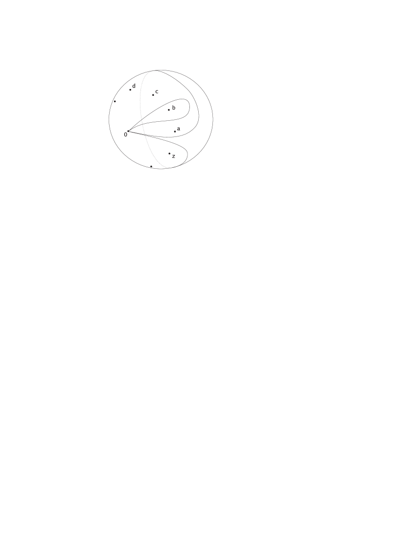
Figure 14: Paths of the monodromy

Another requirement is that the first special sheet is permuted by the first $k_{1}$ loops, the second — by the next $k_{2}$ loops and so on. Finally, we disallow any unramified sheets.

The product of all loops, which is the big loop in Figure 14, is contractible and so the product of the monodromies must be equal to 1. It is clear, that once we choose any labeling of the non-special sheets in the fiber over 0 by the numbers $\{s+1,\dots,n\}$ we get a solution of (3.16) and vice versa. Isomorphic coverings differ by a relabeling of the the non-special sheets and hence the isomorphism classes of coverings correspond to $S(n-s)$-orbits.

We call the covering satisfying these conditions the Jucys-Murphy coverings or JM coverings for short. Let $\mathsf{S}$ be an orientable surface, possibly disconnected. Denote by $\operatorname{Cov}_{\mathsf{S}}(k_{1},\dots,k_{s})$ the set of JM coverings

$$\mathsf{S}\to S^{2}\,.$$

It is clear that if a covering corresponds to a solution $\tau$ of (3.16) then its degree is

$$\deg\left(\mathsf{S}\to S^{2}\right)=s+d(\tau)\,,$$

and the Euler characteristic of $\mathsf{S}$ is equal by Riemann-Hurwitz to

$$\chi(\mathsf{S})=2d(\tau)+2s-|k|\,.$$ (3.18)

Therefore, the formula (3.17) can be restated as

$$\frac{1}{2^{|k|}\,n^{(|k|-s)/2}\,n!}\operatorname{tr}\prod_{i=1}^{s}\widetilde{X}_{i}^{k_{i}}\sim\frac{1}{2^{|k|}}\sum_{\mathsf{S}}n^{(\chi(\mathsf{S})-s)/2}\,\left|\operatorname{Cov}_{\mathsf{S}}(k_{1},\dots,k_{s})\right|\,.$$ (3.19)

Here the sum is over all homeomorphism types of orientable surfaces $\mathsf{S}$, possibly disconnected.

As in the case of (2.5), it is clear that it is sufficient to concentrate on connected surfaces only. If $\mathsf{S}$ is a connected surface of genus $g$ we shall denote the corresponding coverings by $\operatorname{Cov}_{g}(k_{1},\dots,k_{s})$. As always, this set is empty unless $|k|$ is even which we will assume in what follows.

4 Counting coverings

4.1 Main result

4.1.1

In the present section we will prove the following theorem with connects JM coverings $\mathsf{S}\to S^{2}$ with maps on $\mathsf{S}$

Theorem 4

As $k_{i}\to\infty$, we have

$$\left|\operatorname{Cov}_{g}(k_{1},\dots,k_{s})\right|\sim\left|\operatorname{Map}_{g}(k_{1},\dots,k_{s})\right|\,.$$ (4.1)

The proof of this theorem requires some preparations and, in particular, some understanding of the structure of a JM coverings. Before we start these preparations, let us explain how Theorem 4 implies Theorem 1. Then the rest of the section will be devoted devoted to the proof of Theorem 4 and examples.

4.1.2 Proof of Theorem 1

We know that

$$\frac{\left|\operatorname{Map}_{g}(k_{1},\dots,k_{s})\right|}{2^{|k|}}\sim t^{3g-3+3s/2}\,\operatorname{map}_{g}(\xi)\,,\quad k_{i}/t\to\xi_{i}\,,$$

as $k_{i}\to\infty$. Hence if $k_{i}^{\prime}\sim n^{1/3}k_{i}$ then

$$\frac{\left|\operatorname{Cov}_{g}(k_{1},\dots,k_{s})\right|}{2^{|k|}\,n^{g-1+s/2}}\sim\frac{\left|\operatorname{Map}_{g}(k^{\prime}_{1},\dots,k^{\prime}_{s})\right|}{2^{|k^{\prime}|}\,n^{2g-2+s}}\,.$$

I follows that

$$\frac{\left|\operatorname{Cov}_{\mathsf{S}}(k_{1},\dots,k_{s})\right|}{2^{|k|}n^{(s-\chi(\mathsf{S}))/2}}\sim\frac{\left|\operatorname{Map}_{\mathsf{S}}(k^{\prime}_{1},\dots,k^{\prime}_{s})\right|}{2^{|k^{\prime}|}n^{s-\chi(\mathsf{S})}}\,,$$ (4.2)

provided

$$\frac{k_{i}}{n^{1/3}}\,,\,\frac{k^{\prime}_{i}}{n^{2/3}}\to\xi_{i}\,,\quad n\to\infty\,.$$ (4.3)

It will be clear from the proof of Theorem 4 that the right hand side of the following formula (4.4) admits an estimate of the form (2.32) and hence we can apply (4.2) termwise to (2.5) and (3.19),(3.15) to obtain that

$$\frac{1}{2^{|k|}\,n^{(|k|-s)/2}\,n!}\operatorname{tr}\prod_{i=1}^{s}X_{i}^{k_{i}}\sim\frac{1}{2^{|k^{\prime}|}n^{|k^{\prime}|/2}}\left\langle{\prod_{j=1}^{s}\operatorname{tr}H^{k^{\prime}_{i}}}\right\rangle$$ (4.4)

under the provision (4.3). Now comparing (3.14) with the corresponding result for random matrices finishes the proof.

Note that the difference in the exponent of $n$ in (2.5) and (3.19) is responsible for the difference in the scaling in (1.3) and (1.4).

4.1.3 Proof of Theorem 2

Our argument follows the argument of Section 5 in [38]. Consider the following random measures on $\mathbb{R}$

$$\mathcal{X}=\sum_{i}\delta_{x_{i}}\,,\quad\mathcal{Y}=\sum_{i}\delta_{y_{i}}\,,$$

where

$$x_{i}=n^{1/3}\left(\frac{\lambda_{i}}{2n^{1/2}}-1\right)\,,\quad y_{i}=n^{2/3}\left(\frac{E_{i}}{2n^{1/2}}-1\right)\,.$$

Define $\left\langle{\mathcal{X}^{\times s}}\right\rangle$ as the following nonrandom measure on $\mathbb{R}^{s}$

$$\left\langle{\mathcal{X}^{\times s}}\right\rangle(A_{1}\times\cdots\times A_{s})=\left\langle{\prod_{i=1}^{s}\mathcal{X}(A_{i})}\right\rangle\,,$$

and define $\left\langle{\mathcal{Y}^{\times s}}\right\rangle$ similarly. Theorem 1 says that the Laplace transforms of $\left\langle{\mathcal{X}^{\times s}}\right\rangle$ and $\left\langle{\mathcal{Y}^{\times s}}\right\rangle$ have the same limit as $n\to\infty$. Multiply $\left\langle{\mathcal{X}^{\times s}}\right\rangle$ and $\left\langle{\mathcal{Y}^{\times s}}\right\rangle$ by the exponential of the sum of coordinates, which is equivalent to shifting Laplace transform variables by $(1,\dots,1)$. This yields finite measures for which the convergence of Laplace transforms implies weak convergence. Hence all mixed moments of the following random variables

$$\mathcal{X}(A)=|\{y_{i}\in A\}|\,,\quad\mathcal{Y}(A)=|\{y_{i}\in A\}|\,,\quad A\subset[c,\infty)^{s}\,,$$ (4.5)

have identical limits, where $c\in\mathbb{R}$ is arbitrary fixed and $A$ varies. From this one concludes (cf. [38]) that the joint distributions of the random variables (4.5) are the same in the $n\to\infty$ limit. The theorem follows.

4.2 Structure of JM coverings

4.2.1 Valence of nonspecial sheets

Let us make $|k|$ cuts on the sphere from the points $a,\dots,z$ to the infinity as in Figure 15.

Figure 15: Cuts on the sphere

This cuts $\mathsf{S}$ into $(s+d)$ polygons. Let us describe the shape of these polygons and how they fit together.

Given a nonspecial sheet $\sigma$, let its valence be the number of points from $a,\dots,z$ such that the monodromy around that point permutes $\sigma$. Clearly, the valence of every sheet is $\geq 2$. On the other hand

$$\sum_{\text{nonspecial $\sigma$}}(\operatorname{val}(\sigma)-2)=|k|-2d=2s-\chi(\mathsf{S})\,,$$ (4.6)

therefore the number of sheets of valence $\geq 3$ is bounded by $2s-\chi(\mathsf{S})$.

Suppose $\sigma$ is a 2-valent sheet and suppose that the monodromy around one ramification point, say, $p$ permutes it with the 1st special sheet and the monodromy around another ramification point, say, $d$ permutes it with 2nd special sheet. Then the preimages of the cuts in Figure 15 on $\mathsf{S}$ are drawn in Figure 16 where the circled numbers 1 and 2 indicate that the corresponding boundary is attached to the 1st and 2nd special sheet, respectively.

Figure 16: Nonspecial sheet of valence 2

Note how the angles get halved at the points which cover the points $p$ and $d$.

Similarly, if $\sigma$ is a 3-valent sheet then it looks like a triangle (similarly, a sheet of valence $m$ looks like an $m$-gon). For example if monodromies around $q$, $c$, and $k$ permute $\sigma$ with the the 1st, 2nd, and 3rd special sheet, respectively, then $\sigma$ looks like Figure 17.

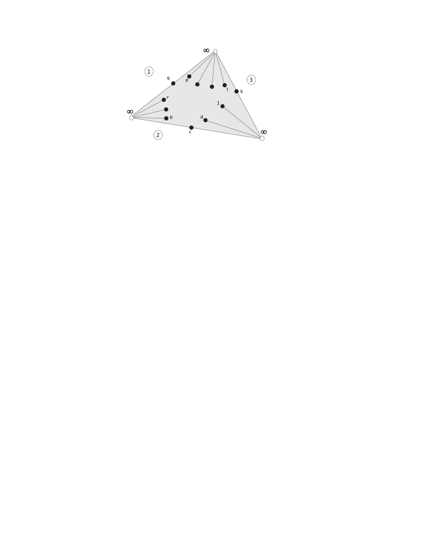
Figure 17: Nonspecial sheet of valence 3

4.2.2 Ribbon graph associated to a covering

The nonspecial sheets naturally glue together at the points which cover $\infty$ to form a ribbon graph whose edges are the 2-valent sheets and vertices are either the sheets of valence $\geq 3$ or multivalent junctions (like in Figure 29) of 2-valent sheets. See Figure 18 and note how $q$ follows $p$ and $d$ follows $c$ after passing through $\infty$.

Figure 18: How nonspecial sheets fit together

Observe, in particular how we have the whole alphabet going once clockwise around each point over $\infty$. This reflects the fact that there is no ramification over $\infty$.

4.2.3 Special sheets

The cells of this ribbon graph correspond to the special sheets and look as follows. Suppose $\sigma$ is the $i$-th special sheet. Then the valence of $\sigma$ is, by construction, equal to $k_{i}$. Suppose that $k_{i}=6$ and the corresponding ramification points are $\{l,m,m,o,p,q\}$. Then this special sheet looks like the hexagon in Figure 19.

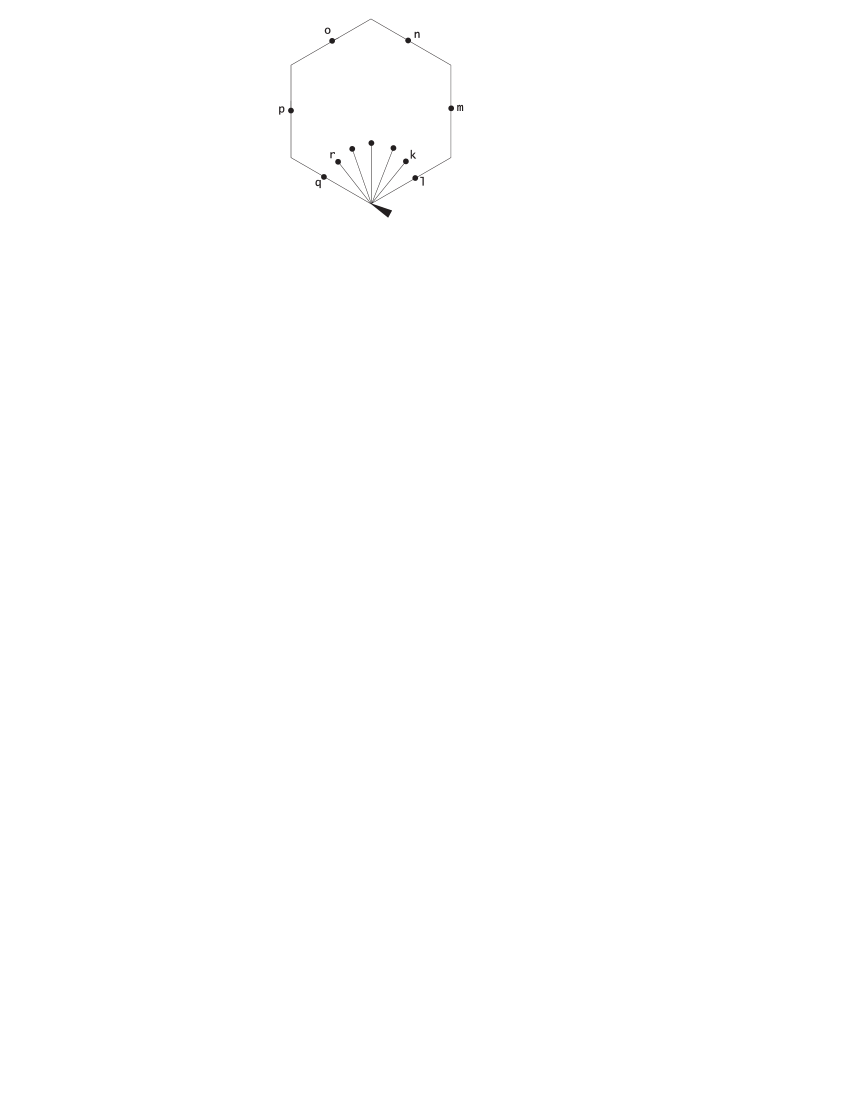
Figure 19: A special sheet with a marked vertex

The special sheets come with a natural choice of the marked vertex, namely, the initial vertex of their first edge in alphabetical order. For example, in Figure 19 the bottom vertex is the marked vertex.

4.2.4 Examples

Consider the following solution to (3.16)

$$(12)(13)(12)(13)(12)(13)=1\,,$$

which is the Coxeter relation in $S(3)$. The corresponding 3-fold covering of the sphere is a torus and the 3 sheets (one 6-valent special, two 3-valent nonspecial) fit together on the torus $T^{2}$ shown in Figure 20.

Figure 20: A 3-fold JM covering $T^{2}\to S^{2}$

4.3 From coverings to maps

4.3.1 The collapsing mapping $\Psi$

We introduce now the following mapping $\Psi$ from JM coverings $\mathsf{S}\to S^{2}$ with $s$ special sheets to maps on $\mathsf{S}$ with $s$ boundary components. What $\Psi$ does is it simply collapses all nonspecial sheets as follows.

If a nonspecial sheet $\sigma$ is 2-valent then we plainly collapse it and glue together the two special sheets which $\sigma$ separated. Nonspecial sheets of valence $\geq 3$ we shrink to the middle as shown in Figure 21 where the collapse of the two nonspecial sheets from Figure 18 is shown (the meaning of the arrow in Figure 21 will be explained below).

Figure 21: Collapse of Figure 18

Note that collapsing a sheet $\sigma$ of valence $\operatorname{val}(\sigma)\geq 3$ increases the length of each of the $\operatorname{val}(\sigma)$ boundaries involved by 1. For example, the boundary in Figure 21 is 3 units longer than the boundary in Figure 18.

The special sheets become the cells of the map, their numbering is just the numbering of the special sheets by $1,\dots,s$ and the marked vertices are the marked vertices of the special sheets.

4.3.2 Example

Note that collapsing the covering discussed in Section 4.2.4 and shown in Figure 20 produces, essentially, the map on torus shown in Figures 6 and 7. More precisely, every edge of this map has length 2 instead of $1$, so the torus is really glued from a 12-on, not from a hexagon.

As another example, consider the equation

$$(12)^{6}=1\,.$$

Which defines a $2$-fold covering of the sphere of genus $2$ with $1$ special and $1$ nonspecial sheet, both $6$-valent. This nonspecial sheet look like a hexagon with 3 nonadjacent vertices glued together and 3 other nonadjacent vertices also glued together. When we collapse this figure to the middle to get the ribbon graph shown in Figure 22.

Figure 22: Ribbon graph corresponding to $(12)^{6}=1$

Its embedding into the genus 2 surface is shown in Figure 23

Figure 23: Embedding of the graph form Figure 22

4.3.3 Left and right vertices

We now observe that ribbon graphs associated to JM covering and the corresponding maps have vertices of two following fundamentally different types. Let $v$ be a vertex of a map. Suppose we are going around the boundary of the 1st polygon counterclockwise, then the around the boundary of the 2nd polygon counterclockwise and so on. We visit our vertex $\operatorname{val}(v)$ times from the $\operatorname{val}(v)$ corners which meet at $v$. We call the vertex $v$ a right vertex if the corners are visited in the clockwise order and a left vertex if the corners are visited in the counterclockwise order. By definition, we call $v$ right if $\operatorname{val}(v)\leq 2$.

Note that if $\operatorname{val}(v)>3$ then $v$ may be neither left nor right. For an example of this, look at the surface of genus 2 obtained by identifying opposite sides of a 10-gon. A left and right vertex of $\operatorname{val}(v)=3$ are shown in Figure 24 where the dashed lines represent the order of going around the three corners.

Figure 24: A left vertex and a right vertex

Suppose $v$ is a vertex of map which came from of a JM covering. Then $v$ either covers $\infty$ or $v$ is the middle point of a collapsed $m$-valent nonspecial sheet where $m\geq 3$. Observe that then $v$ is a right or left vertex, respectively. Indeed, if $v$ covers $\infty$ then, since there is no ramification over $\infty$, the whole alphabet is circling $v$ once clockwise. Similarly, if $v$ was a midpoint of a nonspecial sheet then (see Figure 17) the alphabet was going around $v$ once counterclockwise. This translates into $v$ being a right and left vertex, respectively.

For example, the arrow in Figure 21 shows the order of visiting the corners of the trivalent vertex (which is left). In another example, the graph from Figures 22 and 23 has one 6-valent left vertex and two 3-valent right vertices.

4.3.4 The image of $\Psi$

We call a vertex $v$ an interior vertex if all corners which at meet $v$ come from the same polygon of the map.

We will now prove the following

Proposition 3

The mapping $\Psi$ from JM coverings to maps is one-to-one. Its image $\operatorname{Im}\Psi$ consists of all maps satisfying the two following conditions:

• every vertex is either left of right,

• all marked vertices are interior right vertices,

• the distance between any two left vertices is $\geq 2$.

Recall that for vertices of valence $\geq 4$ being left or right is a nontrivial condition and that is was shown above that only left or right vertices arise from JM coverings.

Proof. By construction, all marked vertices come from some points which cover $\infty$ and, therefore, they are right vertices. Let us show that they also must be interior vertices. This follows from inspection of Figure 25. The Figure 25 shows the marked vertex (the bottom one) of the special sheet from Figure 19.

Figure 25: The marked vertex must be an inner vertex

Since the whole alphabet must go once around $\infty$ the points marked by question marks in Figure 25 cannot be points from $\{r,s,\dots,j,k\}$. On the other hand, the points $\{r,s,\dots,j,k\}$ are precisely the ramification points which do not lie on the boundary of our special sheet. Therefore, all points marked by question marks do lie on the boundary of our special sheet. It follows that all corners in Figure 25 come come from one and the same special sheet.

An algebraic equivalent of this geometric argument is the following. Let $\tau$ be a solution of (3.16). Then $(1\tau_{1})\cdots(1\tau_{k_{1}})$ must fix $1$ because $1$ is clearly fixed by the rest of the product in (3.16). This translates into Figure 25.

We will now show that any map satisfying the above two conditions comes from a unique JM covering. This covering can be reconstructed as follows.

Assign symbols $a,b,c,\dots$ consecutively to all edges of the polygons of the map starting from the marked vertex of the first polygon.

Now consider some vertex $v$ of our map. If $v$ is a right vertex (in particular, if $\operatorname{val}(v)\leq 2$) then the structure of the corresponding JM covering at $v$ can be reconstructed uniquely from the fact that $v$ covers $\infty$ and there is no ramification at $\infty$. (In other words, all letters of the alphabet have to occur once clockwise around $v$).

This reconstruction is shown, respectively, in Figures 26 for the case $\operatorname{val}(v)=1$, in Figure 27 for the case $\operatorname{val}(v)=2$, and in Figures 28 and 29 for $\operatorname{val}(v)=3$.

Figure 26: Reconstruction of JM covering for $\operatorname{val}(v)=1$

Figure 27: Reconstruction of JM covering for $\operatorname{val}(v)=2$

Figure 28: A right vertex of valence $3$

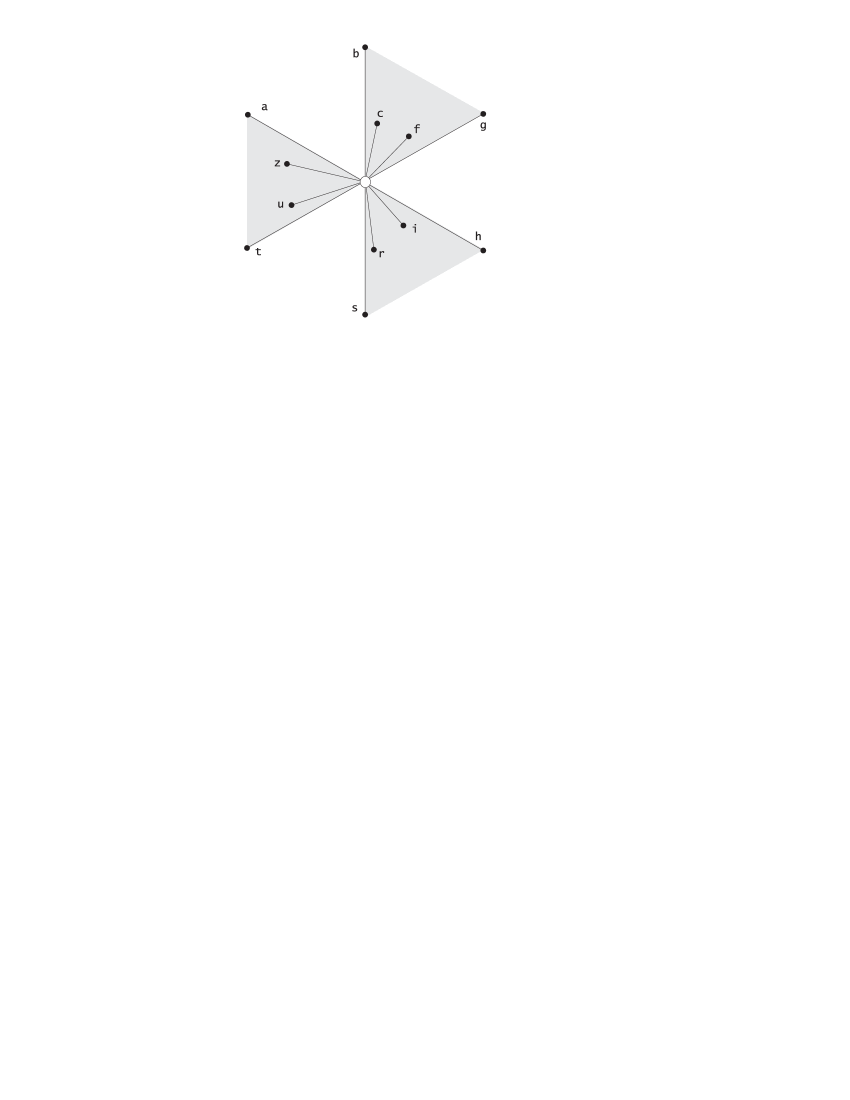
Figure 29: The JM covering corresponding to a right vertex of valence 3

When we encounter a left vertex (such as the vertex with the arrow in Figure 21) then we insert a nonspecial sheet of valence $\operatorname{val}(v)$. The result looks like Figure 17. One should notice that this operation reduces the number of edges by $\operatorname{val}(v)$ and we have to relabel the edges if we want a consecutive alphabetical labeling. Also notice that we have to use the third condition in the statement of the proposition for this reconstruction.

This finishes the reconstruction of nonspecial sheets. As to the special sheets, let us examine the Figure 25. If the edges of a cell of a map are labeled by $l,m,\dots,p,q$ and its initial vertex is an interior right vertex then there is room to fit in the rest of the alphabet as in Figure 25. This concludes the proof.

4.3.5 Example: $s=1$ and $g=0$

Consider the case $s=1$ and $g=0$. The equation (4.6) implies that in this case

$$\sum_{\text{nonspecial $\sigma$}}(\operatorname{val}(\sigma)-2)=2s-2+2g=0\,,$$

and hence there are no nonspecial sheets of valence $>2$. Therefore the map $\Psi$ is a bijection between the sets $\operatorname{Cov}_{0}(k)$ and $\operatorname{Map}_{0}(k)$.

The algebraic translation of this geometric fact is the following. Let

$$(1i_{1})(1i_{2})\dots(1i_{k})=1$$ (4.7)

be the solution of (3.16) corresponding to our covering. By (3.18) the condition $s=1$ , $g=0$ implies that

$$2d(\tau)-|k|=2-2g-2s=0$$

and since every $i_{j}$ has to appear at least twice, this is equivalent to saying that there are precisely $k/2$ pairs of equal numbers among the numbers $i_{1},\dots,i_{k}$.

The bijection $\Psi$ between $\operatorname{Cov}_{0}(k)$ and $\operatorname{Map}_{0}(k)$ and the example in Section 2.2 now mean that (4.7) is satisfied if and only if the the corresponding pairing is noncrossing. This observation is due to P. Biane [4].

Note that the noncrossing in (4.7) means that this equality is a consequence of solely the relations

$$(1i)^{2}=1\,,\quad i=1,2,\dots\,,$$

among the generators $(12),(13),(14),\dots$ of the symmetric group.

4.4 Counting maps

4.4.1

Intoduce the following subsets in $\operatorname{Map}_{g}(k)$, where as usual, we use the abbreviation

$$k=(k_{1},\dots,k_{s})\,.$$

Denote by

$$\operatorname{Map}^{3}_{g}(k)=\Phi^{-1}\left(\Gamma^{3}_{g,s}\right)$$

the set of those maps which after contraction $\Phi$ have only trivalent vertices. Since only trivalent graphs $\Gamma$ contribute to (2.22), we know that

$$\left|\operatorname{Map}^{3}_{g}(k)\right|\sim\left|\operatorname{Map}_{g}(k)\right|\,,\quad k_{i}\to\infty\,.$$ (4.8)

By definition, set

$$\operatorname{Map}^{*}_{g}(k)=\operatorname{Map}^{3}_{g}(k)\,\cap\,\operatorname{Im}\Psi\,,$$

that is, $\operatorname{Map}^{*}_{g}(k)$ is the subset of $\operatorname{Map}^{3}_{g}$ formed by maps satisfying the conditions of Proposition 3. It is the image under $\Psi$ of JM coverings with nonspecial sheets of valence at most $3$.

We will establish the following

Proposition 4

$$\left|\operatorname{Map}^{*}_{g}(k)\right|\sim 2^{-6g+6-6s}\left|\operatorname{Map}^{3}_{g}(k)\right|$$ (4.9)

$$\left|\operatorname{Im}\Psi\cap\operatorname{Map}^{3}_{g}\setminus\operatorname{Map}^{*}_{g}\right|=o\left(\left|\operatorname{Map}^{*}_{g}\right|\right)\,.$$ (4.10)

Once Proposition 4 is established, the Theorem 4 will follow. Indeed, since $\Psi$ is one-to-one, then because of (4.8) and (4.10) it suffices to consider coverings with only $\leq 3$-valent nonspecial sheets. For such a covering, the number of 3-valent sheets equals $2g-2+2s$. Collapsing a trivalent sheet to its middle increases the length of the boundary by 3. Therefore, in total, the boundary of the corresponding map is $6g-6+6s$ longer. Since this precisely compensates the exponent in (4.9), we obtain:

$$\left|\operatorname{Cov}_{g}(k)\right|\sim\left|\operatorname{Map}_{g}(k)\right|\,,\quad k\to\infty\,.$$

We also point out that Proposition 3 gives an upper bound on $|\operatorname{Cov}_{g}(k)|$ which results in an analog of the estimate (2.32) for the right-hand side of (4.4). Indeed, the mapping $\Psi$ is one-to-one and increases the total perimeter of the boundary by at most $6g-6+6s$. From (3.18) we have $g\leq|k|/2$, so the total increase is by at most a multiple of $|k|$ with implies that the right-hand side of (4.4) is again bounded by some function of the $\xi_{i}$’s.

4.4.2 Proof of Proposition 4

In order to examine the difference between the sets $\operatorname{Map}^{3}_{g}$, $\operatorname{Map}^{*}_{g}$, and $\operatorname{Im}\Psi$ we need to introduce the following notions.

Let $v_{0}$ be a marked vertex of a map with $s>1$ polygons. Suppose that $v_{0}$ is an interior vertex. Follow the edges of the corresponding polygon in the counterclockwise direction until we reach a vertex $v$ which is not interior. By analogy with the flow of a river, we call the vertex $v$ a mouth vertex, see Figure 30. Observe that a mouth vertex is never right.

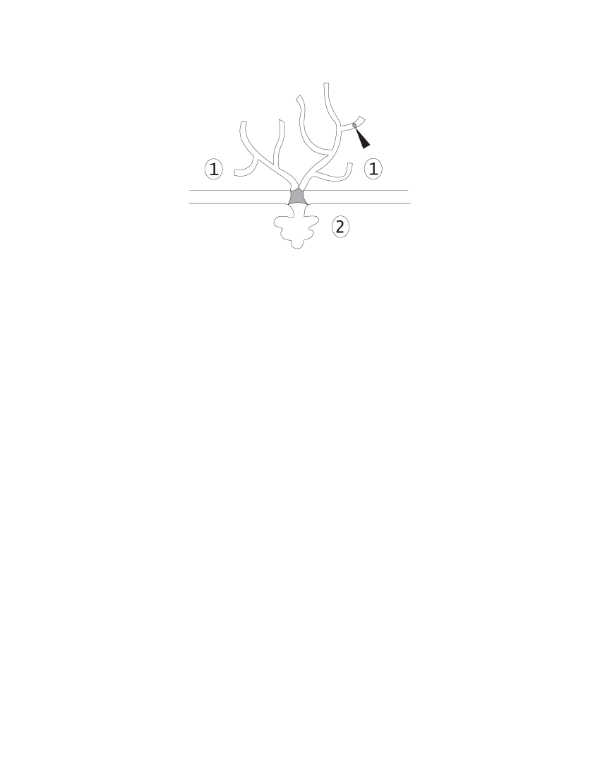
Figure 30: A mouth vertex

Also, call a vertex $v$ of a map contractible if it disappears after contraction of all $\leq 2$-valent vertices; otherwise, call it incontractible. Observe that a contractible vertex is always right unless it is a mouth vertex.

Proof. First, the condition that the marked vertices must be right is asymptotically negligible. Indeed, all but finitely many vertices are right and the chances to hit one them with a mark go to 1 as the perimeter goes to infinity. Similarly, the third condition in Proposition 3 does not affect the asymptotics.

The possible combinatorial configurations of the incontractible and mouth vertices of maps in $\operatorname{Map}^{3}_{g}$ are described by ribbon graphs $\Gamma\in\Gamma^{3}_{g}$ together with the choice of an edge $e_{i}\in e(\Gamma)$, $i=1,\dots,s$, on the boundary of any cell of $\Gamma$. The edge $e_{i}$ is the first edge we reach if we start from the marked vertex of the $i$-th cell of the map. We shall see that, for any configuration, the proportion of maps lying in $\operatorname{Map}^{*}_{g}$ equals $\sim 2^{-6g+6-6s}$, and that the same portion of maps lies in $\operatorname{Im}\Psi$. This number is, in fact, a product of factors $2^{-3}$ over the $2g-2+s$ vertices $v$ that are not right. Let us examine such vertices $v$.

First, suppose $v$ is an incontractible vertex. By definition of $\operatorname{Map}^{3}_{g}$, it means that $v$ becomes trivalent after the 3 trees shown in Figure 31 are contracted onto it.

Figure 31: The forbidden trees of a left vertex

We claim that for such a vertex being left is equivalent to being trivalent. Indeed, suppose $v$ is left and not trivalent. Then, as we go around any nonempty tree in any of the trees shown in Figure 31, we go from one corner of $v$ to the next corner in the clockwise direction. Since $v$ is left, this is impossible.

It follows from the discussion in Sections 2.4 or 2.5.5 that the removal of any given tree comes at the price of the factor $\frac{1}{2}$ in the asymptotics. In terms of the random walk, for example, it means that the first step of the walk has to go up, which is an event of probability $\frac{1}{2}$. Therefore, asymptotically $\sim\frac{1}{2^{3}}$ of maps are trivalent at $v$ or, equivalently, $v$ is a left (or trivalent) vertex for about $\sim\frac{1}{2^{3}}$ of all maps.

Now suppose that $v$ is a contractible mouth vertex, such as the one shown in Figure 30. We may assume that $v$ does not coincide with any other mouth vertex because the chances of such a coincidence vanish as the perimeter of the map goes to infinity.

With this assumption, $v$ being left is again equivalent to $v$ being trivalent and both mean that $v$ must look like the vertex in Figure 32:

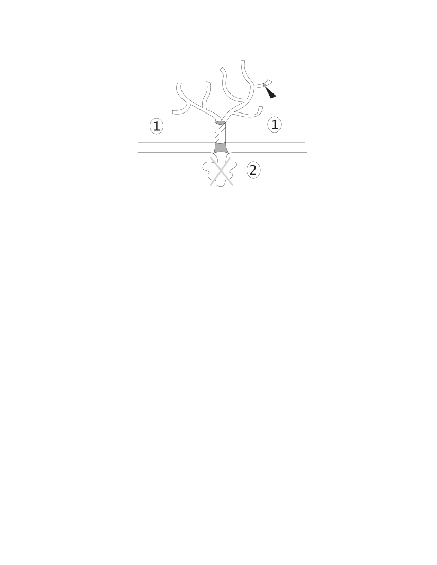
Figure 32: A trivalent contractible mouth vertex

namely, the tree at the bottom must be empty and only one branch (shaded in Figure 32) must go up.

For general maps, multiple branches may go up or no branches at all (which happens if the marked vertex is not interior). Therefore, the insertion of this shaded branch and chopping down the tree at the bottom takes arbitrary maps to maps such that $v$ is a trivalent mouth vertex and the corresponding marked vertex is interior. The insertion of the shaded branch increases the perimeter by $2$. This means that $\sim\frac{1}{2^{2}}$ of maps have it. This times $\frac{1}{2}$ for the forbidden tree gives us the total of $\sim\frac{1}{2^{3}}$ of maps belonging to $\operatorname{Map}^{*}_{g}$.

Either way, we get a factor of $2^{-3}$ for any trivalent left vertex. The number of such vertices can be easily computed. All of them become trivalent nonspecial sheets of the corresponding JM covering. Therefore, by (4.6) there are $2g-2+2s$ of them. This proves (4.9) and (4.10) and concludes the proof of Proposition 4 and, hence, of Theorem 1.

4.5 Example

Note that the noncrossing in (4.7) meant that this equality is a consequence of solely the relations

$$(1i)^{2}=1\,,\quad i=1,2,\dots\,,$$

among the generators $(12),(13),(14),\dots$ of the symmetric group. The relations of Coxeter type (which produce coverings of genus 1)

$$(1i)(1j)(1i)(1j)(1i)(1j)=1$$

start playing role in the enumeration of $\operatorname{Cov}_{1}(k)$.

Every covering in $\operatorname{Cov}_{1}(k)$ has either two 3-valent special sheets or, else, one of valence 4. Consider the first case because the second makes no contribution to the asymptotics. Denote by $\operatorname{Cov}^{3}_{1}(k)$ the corresponding subset of $\operatorname{Cov}_{1}(k)$.

For $\operatorname{Cov}^{3}_{1}(k)$, the corresponding relations are, up to a cyclic shift:

$$(1i)\,w_{1}\,(1j)\,w_{2}\,(1i)\,w_{3}\,(1j)\,w_{4}\,(1i)\,w_{5}\,(1j)\,w_{6}=1$$ (4.11)

Here the $w_{i}$’s are some words in the generators $(12),(13),(14),\dots$ subject to two conditions. First, $(1i)$ and $(1j)$ appear exactly 3 times each in (4.11) and any other generator appears either 0 or 2 times. Second,

$$w_{1}\,w_{4}=w_{2}\,w_{5}=w_{3}\,w_{6}=1\,,$$

which means that any relation (4.11) is built from 3 relations from the $g=0$ case. Using the generating function for the Catalan numbers, one obtains the following generating function

$$\sum_{k}\left|\operatorname{Cov}^{3}_{1}(k)\right|\,z^{k}==\frac{1}{4}\frac{z^{2}\left(1-\sqrt{1-4z^{2}}\right)^{2}}{(1-4z^{2})^{5/2}}\,.$$

Since

$$\frac{1}{4}\frac{z^{2}\left(1-\sqrt{1-4z^{2}}\right)^{2}}{(1-4z^{2})^{5/2}}\sim\frac{1}{16}\frac{1}{(1-4z^{2})^{5/2}}\,,\quad z^{2}\to\frac{1}{4}\,,$$

we conclude that

$$\frac{\left|\operatorname{Cov}_{1}(k)\right|}{2^{k}}\sim\frac{\left|\operatorname{Cov}^{3}_{1}(k)\right|}{2^{k}}\sim\frac{1}{16}\frac{(k/2)^{\frac{5}{2}-1}}{\Gamma(5/2)}=\frac{1}{12\sqrt{\pi}}\left(\frac{k}{2}\right)^{3/2}\,,$$

which agrees with computations of Section 2.6

References

- [1] D. Aldous and P. Diaconis, Hammersley’s interacting particle process and longest increasing subsequences, Prob. Theory and Rel. Fields, 103, 1995, 199–213.
- [2] J. Baik, P. Deift, K. Johansson, On the distribution of the length of the longest increasing subsequence of random permutations, math.CO/9810105.
- [3] J. Baik, P. Deift, K. Johansson, On the distribution of the length of the second row of a Young diagram under Plancherel measure, math.CO/9901118.
- [4] P. Biane, Permutation model for semi-circular systems and quantum random walks, Pacific J. Math., 171, no. 2, 1995, 373–387.
- [5] P. Biane, Representations of symmetric groups and free probability, Adv. Math., 138, 1998, no. 1, 126–181.
- [6] S. Bloch and A. Okounkov, The character of the infinite wedge representation, alg-geom/9712009.
- [7] A. Borodin and G. Olshanski, Distribution on partitions, point processes, and the hypergeometric kernel, math.RT/9904010.
- [8] A. Borodin, A. Okounkov, and G. Olshanski, On asymptotics of the Plancherel measures for symmetric groups, math.CO/9905032.
- [9] P. Diaconis and C. Greene, Applications of Murphy’s elements, Stanford University Technical Report, no. 335, 1989.
- [10] R. Dijkgraaf, Mirror symmetry and elliptic curves, The Moduli Space of Curves, R. Dijkgraaf, C. Faber, G. van der Geer (editors), Progress in Mathematics, 129, Birkhäuser, 1995.
- [11] A. Eskin and A. Okounkov, Branched coverings of the torus and volumes of spaces of Abelian differentials, preprint.
- [12] T. Ekedahl, S. Lando, M. Shapiro, and A. Vainshtein, On Hurwitz numbers and Hodge integrals, math.AG/9902104.
- [13] P. J. Forrester, The spectrum edge of random matrix ensembles, Nuclear Phys. B, 402, 1993, no. 3, 709–728.
- [14] P. Di Francesco, P. Ginsparg, J. Zinn-Justin, gravity and random matrices, Phys. Rep. 254, 1995, 1–133.
- [15] J. Harer and D. Zagier, The Euler characteristic of the moduli space of curves, Invent. Math., 85, 1986, 457–485.
- [16] K. Johansson, The longest increasing subsequence in a random permutation and a unitary random matrix model, Math. Res. Letters, 5, 1998, 63–82.
- [17] K. Johansson, Discrete orthogonal polynomial ensembles and the Plancherel measure, math.CO/9906120.
- [18] A. Jucys, Symmetric polynomials and the center of the symmetric group ring, Reports Math. Phys., 5, 1974, 107–112.
- [19] M. Kontsevich, Intersection theory on the moduli space of curves and the matrix Airy function, Commun. Math. Phys., 147, 1992, 1–23.
- [20] S. Kerov, Gaussian limit for the Plancherel measure of the symmetric group, C. R. Acad. Sci. Paris, 316, Série I, 1993, 303–308.
- [21] S. Kerov, Transition probabilities of continual Young diagrams and the Markov moment problem, Func. Anal. Appl., 27, 1993, 104–117.
- [22] S. Kerov, The asymptotics of interlacing roots of orthogonal polynomials, St. Petersburg Math. J., 5, 1994, 925–941.
- [23] S. Kerov, A differential model of growth of Young diagrams, Proceedings of the St. Petersburg Math. Soc., 4, 1996, 167–194.
- [24] S. Kerov, Interlacing measures, Amer. Math. Soc. Transl., 181, Series 2, 1998, 35–83.
- [25] S. Kerov and A. Okounkov, A new proof of Thoma theorem, unpublished paper, 1995.
- [26] A. Klyachko and E. Kurtaran, Some identities and asymptotics for characters of the symmetric group, J. Algebra, 206, no. 2, 1998, 413–437.
- [27] G. Murphy, A new construction of Young’s seminormal representation of the symmetric group, J. Algebra, 69, 1981, 287–291.
- [28] A. Okounkov, On the representations of the infinite symmetric group, Zapiski Nauchnyh Seminarov POMI, 240, 1997, 167–230, available from math/9803037.
- [29] A. Okounkov, Wick formula, Young basis, and higher Capelli identities, Internat. Math. Res. Notices, 1996, no. 17, 817–839.
- [30] A. Okounkov, Infinite wedge and measures on partitions, math.RT/9907127.
- [31] A. Okounkov, Generating functions for intersection numbers on moduli spaces of curves, in preparation.
- [32] A. Okounkov and A. Vershik, A new approach to representation theory of symmetric groups, Selecta Math. (N.S.), 2, 1996, no. 4, 581–605.
- [33] B. F. Logan and L. A. Shepp, A variational problem for random Young tableaux, Adv. Math., 26, 1977, 206–222.
- [34] Yu. Prohorov and Yu. Rozanov, Probability theory, Springer-Verlag, 1969.
- [35] E. M. Rains, Increasing subsequences and the classical groups, Electr. J. of Combinatorics, 5(1), 1998.
- [36] T. Seppäläinen, A microscopic model for Burgers equation and longest increasing subsequences, Electron. J. Prob., 1, no. 5, 1996.
- [37] Ya. Sinai and A. Soshnikov, A refinement of Wigner’s semicircle law in a neighborhood of the spectrum edge for random symmetric matrices, Func. Anal. Appl., 32, 1998, no. 2, 114–131.
- [38] A. Soshnikov, Universality at the edge of the spectrum in Wigner random matrices, math-ph/9907013.
- [39] C. A. Tracy and H. Widom, Level-spacing distributions and the Airy kernel, Commun. Math. Phys., 159, 1994, 151–174.
- [40] A. Vershik and S. Kerov, Asymptotics of the Plancherel measure of the symmetric group and the limit form of Young tableaux, Soviet Math. Dokl., 18, 1977, 527–531.
- [41] A. Vershik and S. Kerov, Asymptotics of the maximal and typical dimension of irreducible representations of symmetric group, Func. Anal. Appl., 19, 1985, no.1.
- [42] A. Zvonkin, Matrix integrals and map enumeration: an accessible introduction, Math. Comput. Modelling, 26, 1997, no. 8–10, 281–304.