Solving the quintic
by iteration in three dimensions

Abstract.

The requirement for solving a polynomial is a means of breaking its symmetry, which in the case of the quintic, is that of the symmetric group $\mathcal{S}_{5}$. Induced by its five-dimensional linear permutation representation is a three-dimensional projective action. A mapping of complex projective $3$-space with this $\mathcal{S}_{5}$ symmetry can provide the requisite symmetry-breaking tool.

The article describes some of the $\mathcal{S}_{5}$ geometry in $\mathbf{CP}^{3}$ as well as several maps with particularly elegant geometric and dynamical properties. Using a rational map in degree six, it culminates with an explicit algorithm for solving a general quintic. In contrast to the Doyle-McMullen procedure—three $1$-dimensional iterations, the present solution employs one $3$-dimensional iteration.

1. Overview

In [Doyle and McMullen 1989], a solution to the quintic takes place in three iterative steps—a tower of algorithms each of which involves iteration in one complex dimension. Given almost any quintic $p$ and almost any initial point in $\mathbf{C}$, the series of algorithms produces a root of $p$. Their method is geometrically distinguished in that the tower has the $\mathcal{S}_{5}$ symmetry of the general quintic. Its central feature is a map on the Riemann sphere with icosahedral ($\mathcal{A}_{5}$) symmetry.

The present paper describes a solution to a full measure’s worth of quintics that runs as a single iteration in three dimensions. That the procedure produces a root for almost any initial point in complex projective $3$-space ($\mathbf{CP}^{3}$) is conjectural at the moment. At its core is a map on $\mathbf{CP}^{3}$ with $\mathcal{S}_{5}$ symmetry. Motivating this general project is a desire to develop solutions to equations that utilize geometrically elegant dynamical systems.

The work unfolds in three stages: 1) some background geometry, 2) special maps with $\mathcal{S}_{5}$ symmetry, and 3) a solution to the quintic based on the preceding stages.

Section 2: $\mathcal{S}_{5}$ geometry. The setting here is $\mathbf{CP}^{3}$ upon which the symmetric group $\mathcal{S}_{5}$ acts. Finding a map with special $\mathcal{S}_{5}$ geometry requires some familiarity with this action. We will consider some features associated with the maps that emerge in the second stage. Indeed, the discovery of these maps derives from an awareness of the geometric landscape:

• coordinate systems

• the structure of an $\mathcal{S}_{5}$-invariant quadric surface

• the structure of certain special orbits of points, lines, planes, and conics.

In addition, the system of $\mathcal{S}_{5}$-invariant polynomials plays a fundamental role in the search for maps.

Section 3: Maps with $\mathcal{S}_{5}$ symmetry. At this stage, we exploit our geometric understanding to discover empirically several maps with special qualities. Appearing here are families of maps associated with the icosahedron, the dodecahedron, and the complete graph on five vertices. The known features of their geometric and dynamical behavior come under discussion. However, they are not known to possess several desired properties. In light of significant experimental evidence, I leave claims concerning these properties as conjectures.

Section 4: Dynamical solution to the quintic. Following the Doyle-McMullen framework, a special family of quintics corresponds to a rigid family $\mathcal{E}$ of $\mathcal{S}_{5}$ maps on $\mathbf{CP}^{3}$. ‘Rigidity’ means that each member of $\mathcal{E}$ is conjugate to a single reference map $f$ with elegant geometry and dynamics. The solution is general since almost any quintic $p$ transforms into the special family. Thus, associated with $p$ is a map $g$ that we iterate. Using $\mathcal{S}_{5}$ tools, its output—conjecturally, a single $\mathcal{S}_{5}$ orbit—provides for an approximate solution to $\{p=0\}$.

A subsequent paper extends the method to the octic in a way that might generalize to higher degree. [Crass 1999c]

2. $\mathcal{S}_{5}$ acts on $\mathbf{CP}^{3}$

The permutation action of the $\mathcal{S}_{5}$ on $\mathbf{C}^{5}$ preserves the hyperplane

$$\mathcal{H}_{x}=\Biggl{\{}\sum_{k=1}^{5}x_{k}=0\Biggr{\}}\simeq\mathbf{C}^{4}$$

and, thereby, restricts to a faithful four-dimensional irreducible representation. (Since there will be two variables that describe the hyperplane, the subscript $x$ appears here.) This induces an $\mathcal{S}_{5}$ action on $\mathbf{CP}^{3}$. Let $\mathcal{G}_{120}$ denote the corresponding subgroup of $\text{PGL}_{4}\mathbf{C}$.

2.1. Coordinates

For many purposes, the most perspicuous geometric description of $\mathcal{G}_{120}$ employs five coordinates that sum to zero. One advantage is the simple expression of the $\mathcal{G}_{120}$-duality between points and planes. In general, for a finite action $\mathcal{G}$ whose matrix representatives are unitary, a point $a$ is $\mathcal{G}$-dual to a hyperplane $\mathcal{L}$ if

$$\mathcal{L}=\{\overline{a}\cdot x=0\}.$$

Consequently, $a$ and $\mathcal{L}$ have the same stabilizer in $\mathcal{G}$. By the orthogonal action of $\mathcal{S}_{5}$ on $\mathbf{C}^{4}$, a point

$$a=[a_{1},a_{2},a_{3},a_{4},a_{5}]_{\sum a_{k}=0}\in\mathbf{CP}^{3}$$

corresponds to the plane

$$\{a\cdot x=0\}=\Biggl{\{}\sum_{k=1}^{5}a_{k}\,x_{k}=0\Biggr{\}}.$$

(Square brackets indicate a point in projective space.)

A system of four $u$-coordinates also describes the hyperplane $\mathcal{H}_{u}$. These hyperplane coordinates arise from the “hermitian” change of variable

$$u=H\,x\quad x=\overline{H^{T}}u\quad H=\frac{1}{\sqrt{5}}\left(\begin{array}[]{ccccc}1&\mathbf{\omega}_{5}&\mathbf{\omega}_{5}^{2}&\mathbf{\omega}_{5}^{3}&\mathbf{\omega}_{5}^{4}\\ 1&\mathbf{\omega}_{5}^{2}&\mathbf{\omega}_{5}^{4}&\mathbf{\omega}_{5}&\mathbf{\omega}_{5}^{3}\\ 1&\mathbf{\omega}_{5}^{3}&\mathbf{\omega}_{5}&\mathbf{\omega}_{5}^{4}&\mathbf{\omega}_{5}^{2}\\ 1&\mathbf{\omega}_{5}^{4}&\mathbf{\omega}_{5}^{3}&\mathbf{\omega}_{5}^{2}&\mathbf{\omega}_{5}\end{array}\right)$$

where $\mathbf{\omega}_{5}=e^{2\,\pi\,i/5}$ and the choice of scalar factor gives

(1) $$H\,\overline{H^{T}}=\begin{pmatrix}1&0&0&0\\ 0&1&0&0\\ 0&0&1&0\\ 0&0&0&1\end{pmatrix}\quad\overline{H^{T}}H=-\begin{pmatrix}-4&1&1&1&1\\ 1&-4&1&1&1\\ 1&1&-4&1&1\\ 1&1&1&-4&1\\ 1&1&1&1&-4\end{pmatrix}.$$

2.2. Invariant polynomials

The fundamental result on symmetric functions states that the $n$ elementary symmetric functions of degrees one through $n$ generate the ring of $\mathcal{S}_{n}$-invariant polynomials. Since the $\mathcal{S}_{5}$ action on $\mathbf{CP}^{3}$ occurs where the degree-$1$ symmetric polynomial vanishes, there are four generating $\mathcal{G}_{120}$-invariants. By Newton’s identities, the power sums

$$F_{k}(x)=\sum_{\ell=1}^{5}x_{\ell}^{k}\qquad k=2,\dots,5$$

also generate the $\mathcal{G}_{120}$ invariants. In hyperplane coordinates, these are

$$\Phi_{2}(u)= \ F_{2}(\overline{H^{T}}u)=2\,\bigl{(}u_{1}\,u_{4}+u_{2}\,u_{3}\bigr{)}$$

$$\Phi_{3}(u)= \ \frac{3}{\sqrt{5}}\,\bigl{(}u_{1}\,u_{2}^{2}+u_{1}^{2}\,u_{3}+u_{3}^{2}\,u_{4}+u_{2}\,u_{4}^{2}\bigr{)}$$

$$\Phi_{4}(u)= \ \frac{2}{5}\,\bigl{(}2\,u_{1}^{3}\,u_{2}+3\,u_{2}^{2}\,u_{3}^{2}+2\,u_{1}\,u_{3}^{3}+2\,u_{2}^{3}\,u_{4}+12\,u_{1}\,u_{2}\,u_{3}\,u_{4}+3\,u_{1}^{2}\,u_{4}^{2}+2\,u_{3}\,u_{4}^{3}\bigr{)}$$

$$\Phi_{5}(u)= \ \frac{1}{5\,\sqrt{5}}\,\bigl{(}u_{1}^{5}+u_{2}^{5}+20\,u_{1}\,u_{2}^{3}\,u_{3}+30\,u_{1}^{2}\,u_{2}\,u_{3}^{2}+u_{3}^{5}+30\,u_{1}^{2}\,u_{2}^{2}\,u_{4}$$

$$+20\,u_{1}^{3}\,u_{3}\,u_{4}+20\,u_{2}\,u_{3}^{3}\,u_{4}+30\,u_{2}^{2}\,u_{3}\,u_{4}^{2}+30\,u_{1}\,u_{3}^{2}\,u_{4}^{2}+20\,u_{1}\,u_{2}\,u_{4}^{3}+u_{4}^{5}\bigr{)}.$$

In classical invariant theory, relative invariants result from taking the determinant of 1) the hessian $H(F)$ of an invariant $F$ and 2) the “bordered hessian” $B(F,G)$ of two invariants $F$ and $G$

$$B(F,G)=\begin{pmatrix}&&&\frac{\partial{G}}{\partial{x_{1}}}\\ &H(F)&&\vdots\\ &&&\frac{\partial{G}}{\partial{x_{n}}}\\ \frac{\partial{G}}{\partial{x_{1}}}&\dots&\frac{\partial{G}}{\partial{x_{n}}}&0\end{pmatrix}.$$

A polynomial $F$ is relatively invariant if, for all $T\in\mathcal{G}$,

$$F\circ T=\alpha_{T}\,F$$

where $\alpha$ is a character on $\mathcal{G}$.

Proposition 1.

Given $T\in\mathrm{GL}_{n}(\mathbf{C})$ and invariants $F,G$,

$$|H(F(Tx))|= \ |T|^{-2}\,|H(F(x))|$$

$$|B(F(Tx),G(Tx))|= \ |T|^{-2}\,|B(F(x),G(x))|.$$

Here, $|\cdot|$ indicates the determinant.

For the permutation action of $\mathcal{S}_{5}$, these give absolute invariants—the character is trivial. Thus, each is expressible in terms of the generators $\Phi_{k}$. The following result will serve a subsequent computational purpose. (Note: Many of this work’s results derive from calculation. For this purpose, I used Mathematica. I will refer to them as “Facts.” )

Fact 1.

With $G_{4}=|H(\Phi_{3})|$ and $G_{5}=|B(\Phi_{3},\Phi_{2})|$, the “power-sum” invariants of degrees four and five are given by

$$\Phi_{4}= \ \frac{1}{324}\bigl{(}\Phi_{2}^{2}-5\,G_{4}\bigr{)}$$

$$\Phi_{5}= \ \frac{1}{864}\bigl{(}720\,\Phi_{2}\,\Phi_{3}+G_{5}\bigr{)}.$$

2.3. Quadric surface

The degree-$2$ invariant defines an $\mathcal{S}_{5}$-invariant surface in $\mathbf{CP}^{3}$

$$\mathcal{Q}=\{\Phi_{2}=0\}.$$

The quadratic form associated with $\mathcal{Q}$ is given by

$$\Phi_{2}=2\,\det U\quad\text{with}\quad U=\begin{pmatrix}u_{1}&-u_{2}\\ u_{3}&u_{4}\end{pmatrix}.$$

Accordingly, $\mathcal{Q}$ is ruled by two families of lines

$$a^{T}\,U=\begin{pmatrix}a_{1}&a_{2}\end{pmatrix}\begin{pmatrix}u_{1}&-u_{2}\\ u_{3}&u_{4}\end{pmatrix}=\begin{pmatrix}0&0\end{pmatrix}\quad U\,b=\begin{pmatrix}u_{1}&-u_{2}\\ u_{3}&u_{4}\end{pmatrix}\begin{pmatrix}b_{1}\\ b_{2}\end{pmatrix}=\begin{pmatrix}0\\ 0\end{pmatrix}.$$

Alternatively, the “$a$-ruling” is defined by

$$U^{T}a=0.$$

Each ruling forms a projective line $\mathbf{CP}^{1}_{a},\ \mathbf{CP}^{1}_{b}$ respectively.

Given a point $u=[u_{1},u_{2},u_{3},u_{4}]$ on $\mathcal{Q}$, the matrices $U$ and $U^{T}$ each have rank one. Thus, distinct lines in $\mathbf{CP}^{1}_{a}$ (or $\mathbf{CP}^{1}_{b}$) are skew while exactly one $a$-line and one $b$-line intersect at $u$. This gives the quadric a $\mathbf{CP}^{1}_{a}\times\mathbf{CP}^{1}_{b}$ structure. (See [Hodge and Pedoe 1968], Ch. XIII: Quadrics.)

Furthermore, as a set, each ruling has an $\mathcal{A}_{5}$ stabilizer $\mathcal{G}_{60}$ and, hence, $\mathbf{CP}^{1}_{a}$ and $\mathbf{CP}^{1}_{b}$ have icosahedral geometry. The “odd” elements $\mathcal{G}_{120}-\mathcal{G}_{60}$ exchange the $a$-ruling with the $b$-ruling.

2.4. Special orbits

The $3$-dimensional $\mathcal{S}_{5}$ action comes in both real and complex versions. This means that, in the standard $x$ coordinates, $\mathcal{G}_{120}$ acts on $\mathcal{R}$—the $\mathbf{RP}^{3}$ of points with real components. Table 1 in Appendix A enumerates some special orbits contained in $\mathcal{R}$ while Table 2 describes elements of $\mathcal{Q}$ that are fixed by members of $\mathcal{G}_{120}$. For ease of expression, I will refer to special points (or lines, planes, etc.) in terms of the orbit size: “$20$-points” ($10$-lines, $5$-planes). Also, these points get a symbolic description in reference to orbit size (superscript) and coordinate expression (subscript).

Corresponding to each special point $a$ is the plane $\{a\cdot x=0\}$. In the case of the 10-points

$$[1,-1,0,0,0],\ \dots\ ,[0,0,0,1,-1],$$

there are 10-planes

$$\{x_{1}=x_{2}\},\ \dots\ ,\{x_{4}=x_{5}\}$$

that are pointwise fixed by the involutions

$$x_{1}\leftrightarrow x_{2},\ \dots\ ,x_{4}\leftrightarrow x_{5}.$$

These ten transpositions generate $\mathcal{G}_{120}$ making it the projective image of a real or complex reflection group. (See [Shephard and Todd 1954].)

Another noteworthy orbit is that of the five $\mathcal{S}_{4}$-stable coordinate planes

$$\mathcal{L}^{2}_{5_{i}}=\{x_{i}=0\}\quad i=1,\dots,5$$

as well as the five octahedral conics

$$\mathcal{Q}^{1}_{i}=\mathcal{Q}\cap\mathcal{L}^{2}_{5_{i}}.$$

Some data for special two-dimensional orbits appear in Table 3. I describe these sets in terms of dimension (superscript), orbit-size (subscript), and coordinate expression (sub-subscript).

Finally, a number of special lines appear as intersections of the $5$-planes and $10$-planes. Table 4 summarizes the situation.

2.5. Configurations

Some of the geometry that will have dynamical significance shows up in various collections of lines. First, the 10-lines

$$\mathcal{M}^{1}_{10_{ijk}}=\mathcal{L}^{2}_{10_{ij}}\cap\mathcal{L}^{2}_{10_{ik}}\cap\mathcal{L}^{2}_{10_{jk}}$$

form a complete graph on the 5-points. Figure 1 illustrates this in two ways. The pentagon-pentagram figure displays a $5$-fold symmetry while the double pyramid exhibits the $\mathcal{D}_{3}$ structure of a single $10$-line. (The illustration suppresses the ‘10’ subscript.)

The intersections of “complementary” pairs of 10-planes yield an orbit of 15-lines

$$\mathcal{L}^{1}_{15_{ij,k\ell}}=\mathcal{L}^{2}_{10_{ij}}\cap\mathcal{L}^{2}_{10_{k\ell}}\qquad\{i,j\}\cap\{k,\ell\}=\emptyset.$$

This forms a graph on 15 vertices—the 5-points and 10-points $p^{10}_{ij_{2}}$.

• At a 5-point $p^{5}_{i}$, there are three 15-lines

  $$\mathcal{L}^{1}_{15_{jk,\ell m}},\mathcal{L}^{1}_{15_{j\ell,km}},\mathcal{L}^{1}_{15_{jm,k\ell}}\quad i\neq j,k,\ell,m.$$

• On a 15-line $\mathcal{L}^{1}_{15_{jk,\ell m}}$, there is one 5-point $p^{5}_{i}$ where $i\neq j,k,\ell,m$.

• At a 10-point $p^{10}_{ij_{2}}$, there are three 15-lines

  $$\mathcal{L}^{1}_{15_{ij,k\ell}},\mathcal{L}^{1}_{15_{ij,km}},\mathcal{L}^{1}_{15_{ij,\ell m}}.$$

• On a 15-line $\mathcal{L}^{1}_{15_{ij,k\ell}}$ there are two 10-points $p^{10}_{ij_{2}}$, $p^{10}_{k\ell_{2}}$.

Within each of the icosahedral rulings on $\mathcal{Q}$ there are three special line-orbits. These correspond to the 12 vertices, 20 face-centers, and 30 edge-midpoints of the icosahedron. Intersections of lines between rulings give special point structures.

• Two $20$-line $\mathcal{G}_{60}$-orbits form ten “quadrilaterals” at two pairs of $20$-points. (See Figure 2.)

• Two $12$-line $\mathcal{G}_{60}$-orbits form six quadrilaterals at $24$-points.

• Two $30$-line $\mathcal{G}_{60}$-orbits orbits form $15$ quadrilaterals at two pairs of $30$-points.

Since $\mathcal{G}_{120}-\mathcal{G}_{60}$, exchanges the orbits in $\mathbf{CP}^{1}_{a}$ with those in $\mathbf{CP}^{1}_{b}$, these give overall line-orbits of sizes $40$, $24$, and $60$.

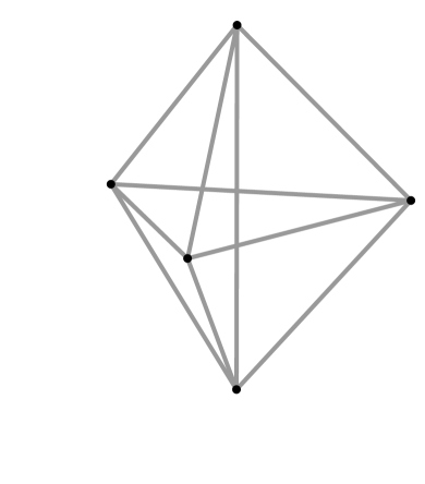
Figure 1. Configuration of $10$-lines and $5$-points

Figure 2. Configuration of $40$-lines and $20$-points on $\mathcal{Q}$. At a $20$-point $q^{20}_{ij_{-}}$ or $q^{20}_{ijk_{-}}$ there are two $40$-lines—one in each ruling on the quadric. This pair of lines is the intersection of $\mathcal{Q}$ with the tangent plane to $\mathcal{Q}$ at the respective $20$-point. Also indicated are the $10$-lines determined by a pair of antipodal $20$-points.

3. Equivariant maps

The primary tool to be used in solving the general quintic is a rational map

$$f:\mathbf{CP}^{3}\longrightarrow\mathbf{CP}^{3}$$

with $\mathcal{S}_{5}$ symmetry. In algebraic terms, this means that

$$f\circ T=T\circ f\quad\text{for all}\ T\in\mathcal{G}_{120}.$$

Furthermore, such an equivariant map (or simply equivariant) should have reliable dynamics: its attractor

1. is a single $\mathcal{G}_{120}$ orbit

2. has a corresponding basin with full measure in $\mathbf{CP}^{3}$

3. alternatively, has a corresponding basin that is dense in $\mathbf{CP}^{3}$.

Recall that a point $a$ in a space $X$ is attracting when, for all $x$ in some neighborhood of $a$,

$$f^{k}(x)\longrightarrow a.$$

A point $s$ is superattracting in a direction $L$ if the derivative $f^{\prime}(s)$ has a zero eigenvalue in the $L$ direction. The basin of attraction $B_{a}$ of $a$ is the set of all points attracted to $a$;

$$B_{a}=\{x\in X:f^{k}(x)\longrightarrow a\}.$$

Also, the attractor of $f$ is the set of all attracting points.

3.1. Basic maps

A finite group action $\mathcal{G}$ on $\mathbf{C}^{n}$ induces an action on the associated exterior algebra. Moreover, $\mathcal{G}$-invariant $(n-1)$-forms correspond to $\mathcal{G}$-equivariant maps. [Crass forthcoming] Briefly, let

$$dZ^{I}=(-1)^{\sigma_{I}}dz_{i_{1}}\wedge\dots\wedge dz_{i_{n-1}}$$

where $I$ is the ordered set

$$\{i_{1},\dots,i_{n-1}\}\qquad i_{1}<\dots<i_{n-1},$$

$\hat{I}$ is the single index in $\{1,\dots,n\}-I,$ and $\sigma_{I}$ is the sign of the permutation

$$\begin{pmatrix}1&2&\dots&n\\ \hat{I}&i_{1}&\dots&i_{n-1}\end{pmatrix}.$$

If

$$\phi(z)=\sum_{\hat{I}=1}^{n}f_{\hat{I}}(z)dz^{I}$$

is a $\mathcal{G}$-invariant $(n-1)$-form, then the map

$$f(z)=(f_{1}(z),\dots,f_{n}(z))$$

is relatively $\mathcal{G}$-equivariant (a multiplicative character appears under the action of $\mathcal{G}$ on $f$).

For a reflection group, the number of generating $0$-forms (i.e., polynomials) is the dimension of the action. [Shephard and Todd 1954, p. 282] From a result in complex reflection groups, this is also the number of generating $1$-forms and $(n-1)$-forms. [Orlik and Terao 1992, p. 232] Indeed, the $1$-forms are exterior derivatives of the $0$-forms while the $(n-1)$-forms are wedge products of $1$-forms.

Proposition 2.

With $X^{k}_{i}=-4\,x_{i}^{k}+\sum_{j\neq i}x_{j}^{k}$, the four maps

$$f_{k}(x)=\bigl{[}X^{k}_{1},X^{k}_{2},X^{k}_{3},X^{k}_{4},X^{k}_{5}\bigr{]}\qquad k=1,\dots,4$$

generate the module of $\mathcal{G}_{120}$ equivariants over the ring of $\mathcal{G}_{120}$-invariants.

These maps are projections onto the hyperplane $\mathcal{H}_{x}$ along $[1,1,1,1,1]$ of the power maps

$$\bigl{[}x_{1}^{k},x_{2}^{k},x_{3}^{k},x_{4}^{k},x_{5}^{k}\bigr{]}.$$

Proposition 3.

Under an orthogonal action an invariant $F(x)$ gives rise to an equivariant $f(x)$ by means of a formal gradient

$$f(x)=\nabla_{x}F(x)=\biggl{[}\frac{\partial F}{\partial x_{1}}(x),\dots,\frac{\partial F}{\partial x_{n}}(x)\biggr{]}.$$

Proof.

For a homogeneous polynomial $F(x)$ of degree $m$, the Euler identity gives

$$m\,F(x)=\nabla_{x}F(x)^{T}x=\nabla_{x}F(x)\cdot x=f(x)\cdot x.$$

Invariance of $F$ yields

$$m\,F(x)=m\,F(Ax)=\nabla_{x}F(Ax)^{T}Ax.$$

Using an auxiliary variable $y$,

$$\nabla_{x}F(Ax)=A^{T}\,\nabla_{y}F(y)|_{y=A\,x}=A^{T}\,f(y)=A^{T}\,f(A\,x).$$

By orthogonality of $A$,

$$m\,F(x)=A^{-1}\,f(A\,x)\cdot x.$$

Equating expressions for $m\,F(x)$ reveals equivariance:

$$A^{-1}f(Ax)=f(x).$$

∎

Note that the $\mathcal{S}_{5}$-equivariant $f_{k}(x)$ is not equal to $\nabla_{x}F_{k+1}(x)$, but is a multiple of

$$\nabla F_{k+1}(x)|_{x_{i}^{k}=X_{i}^{k}}.$$

While this may be a source of confusion, it does not cause problems, since we are working on the hyperplane $\mathcal{H}_{x}$. When using hyperplane coordinates on $\mathcal{H}_{u}$, the discrepancy disappears.

A map on $\mathcal{H}_{x}$ produces

$$\phi(u)=Hf(\overline{H^{T}}u)$$

on $\mathcal{H}_{u}$. Expressing the generating $u$-equivariants

$$\phi_{k}(u)=Hf_{k}(\overline{H^{T}}u)$$

in terms of the basic $u$-invariants $\Phi_{k}(u)$ will be useful.

Definition 1.

Let

$$R=\begin{pmatrix}0&0&0&1\\ 0&0&1&0\\ 0&1&0&0\\ 1&0&0&0\end{pmatrix}\quad\text{and}\quad\nabla_{u}^{r}F(u)=R\,\nabla_{u}F(u)$$

represent the reversed identity and reversed gradient.

Proposition 4.

In $\mathcal{H}_{u}$ coordinates, the map $\phi(u)=H\,f(\overline{H^{T}}u)$ is given by

$$\phi(u)=\nabla_{u}^{r}\Phi(u)$$

where $\Phi(u)=F(\overline{H^{T}}u)=F(x)$.

Proof.

For the change of variable $u=H\,x$ and $x=\overline{H^{T}}\,u$, the chain rule yields

$$f(x)=\nabla_{x}F(x)=\nabla_{x}\Phi(u)=H^{T}\,\nabla_{u}\Phi(u).$$

Since $HH^{T}=R$,

$$H\,f(x)= \ H\,H^{T}\,\nabla_{u}\Phi(u)$$

$$H\,f(\overline{H^{T}}\,u)= \ R\,\nabla_{u}\Phi(u)$$

$$\phi(u)= \ \nabla_{u}^{r}\Phi(u).$$

∎

Thus, the basic maps in $u$ are

$$\phi_{k}(u)=-\frac{5}{k+1}\,\nabla_{u}^{r}\Phi_{k+1}(u).$$

Explicitly,

$$\phi_{1}(u)= \ 2\,\bigl{[}u_{1},u_{2},u_{3},u_{4}\bigr{]}$$

$$\phi_{2}(u)= \ \frac{3}{\sqrt{5}}\,\bigl{[}u_{3}^{2}+2\,u_{2}\,u_{4},u_{1}^{2}+2\,u_{3}\,u_{4},2\,u_{1}\,u_{2}+u_{4}^{2},u_{2}^{2}+2\,u_{1}\,u_{3}\bigr{]}$$

$$\phi_{3}(u)= \ \frac{4}{5}\,\bigl{[}u_{2}^{3}+6\,u_{1}\,u_{2}\,u_{3}+3\,u_{1}^{2}\,u_{4}+3\,u_{3}\,u_{4}^{2},3\,u_{2}^{2}\,u_{3}+3\,u_{1}\,u_{3}^{2}+6\,u_{1}\,u_{2}\,u_{4}+u_{4}^{3},$$

$$u_{1}^{3}+3\,u_{2}\,u_{3}^{2}+3\,u_{2}^{2}\,u_{4}+6\,u_{1}\,u_{3}\,u_{4},3\,u_{1}^{2}\,u_{2}+u_{3}^{3}+6\,u_{2}\,u_{3}\,u_{4}+3\,u_{1}\,u_{4}^{2}\bigr{]}$$

$$\phi_{4}(u)= \ \frac{6}{\sqrt{5}}\,\bigl{[}4\,u_{1}^{2}\,u_{2}^{2}+4\,u_{1}^{3}\,u_{3}+4\,u_{2}\,u_{3}^{3}+12\,u_{2}^{2}\,u_{3}\,u_{4}+12\,u_{1}\,u_{3}^{2}\,u_{4}+12\,u_{1}\,u_{2}\,u_{4}^{2}+u_{4}^{4},$$

$$4\,u_{1}\,u_{2}^{3}+12\,u_{1}^{2}\,u_{2}\,u_{3}+u_{3}^{4}+4\,u_{1}^{3}\,u_{4}+12\,u_{2}\,u_{3}^{2}\,u_{4}+6\,u_{2}^{2}\,u_{4}^{2}+12\,u_{1}\,u_{3}\,u_{4}^{2},$$

$$u_{2}^{4}+12\,u_{1}\,u_{2}^{2}\,u_{3}+6\,u_{1}^{2}\,u_{3}^{2}+12\,u_{1}^{2}\,u_{2}\,u_{4}+4\,u_{3}^{3}\,u_{4}+12\,u_{2}\,u_{3}\,u_{4}^{2}+4\,u_{1}\,u_{4}^{3},$$

$$u_{1}^{4}+4\,u_{2}^{3}\,u_{3}+12\,u_{1}\,u_{2}\,u_{3}^{2}+12\,u_{1}\,u_{2}^{2}\,u_{4}+12\,u_{1}^{2}\,u_{3}\,u_{4}+6\,u_{3}^{2}\,u_{4}^{2}+4\,u_{2}\,u_{4}^{3}\bigr{]}.$$

3.2. A fixed point property

For a $\mathcal{G}_{120}$-equivariant $f$ and a point $a$ that an element $T\in\mathcal{G}_{120}$ fixes,

$$T\,f(a)=f(Ta)=f(a).$$

Hence, equivariants preserve fixed points of a group element.

Being pointwise fixed by the involution

$$x_{i}\longleftrightarrow x_{j},$$

a $10$-plane

$$\mathcal{L}^{2}_{10_{ij}}=\{x_{i}-x_{j}=0\}$$

either maps to itself or collapses to its companion $10$-point

$$p^{10}_{ij_{1}}=[\dots 0\dots,\overbrace{1}^{i},\dots 0\dots,\overbrace{-1}^{j},\dots 0\dots]\notin\mathcal{L}^{2}_{10_{ij}}.$$

In the former generic case, the map preserves the $10$-line and $15$-line orbits $\mathcal{M}^{1}_{10_{ij}}$ and $\mathcal{L}^{1}_{15_{ij,k\ell}}$ that are intersections of $10$-planes.

3.3. Families of equivariants

The $\mathcal{G}_{120}$ equivariants form a module over the $\mathcal{G}_{120}$ invariants for which degree provides a grading. This means that for an invariant $F_{\ell}$ and equivariant $g_{m}$ of degrees $\ell$ and $m$, the product

$$F_{\ell}\cdot g_{m}$$

is an equivariant of degree $\ell+m$. When looking for a map in a certain degree $k$ with special geometric or dynamical properties, my approach is to express the entire family of “$k$-maps” and by manipulation of parameters, locate a subfamily with the desired behavior.

3.4. Quadric-preserving maps

The rich geometry of the quadric $\mathcal{Q}$ provides an intriguing setting for dynamical exploration. Are there $\mathcal{S}_{5}$-symmetric maps that send $\mathcal{Q}$ to itself? If so, how do they behave on and off $\mathcal{Q}$? I will describe discoveries of two species of such maps: one associated with the icosahedron and the other with the octahedron.

Maps that preserve icosahedral rulings

Were a $\mathcal{G}_{120}$-equivariant to preserve the $\mathcal{A}_{5}$ rulings on $\mathcal{Q}$, its restriction to either ruling $\mathbf{CP}^{1}_{a}$ or $\mathbf{CP}^{1}_{b}$ would express itself in terms of the basic equivariants under the one-dimensional icosahedral action. Such maps occur in degrees $11$, $19$, and $29$. [Doyle and McMullen 1989, p. 166] Consequently, the $20$-parameter family of $11$-maps comes under scrutiny:

$$f_{11}=\ (\alpha_{1}\,F_{2}^{5}+\alpha_{2}F_{2}^{2}\,F_{3}^{2}+\alpha_{3}\,F_{2}^{3}\,F_{4}+\alpha_{4}\,F_{3}^{2}\,F_{4}+\alpha_{5}\,F_{2}\,F_{4}^{2}+\alpha_{6}\,F_{2}\,F_{3}\,F_{5}+\alpha_{7}\,F_{5}^{2})\,f_{1}$$

$$+(\alpha_{8}\,F_{2}^{3}\,F_{3}+\alpha_{9}\,F_{3}^{3}+\alpha_{10}\,F_{2}\,F_{3}\,F_{4}+\alpha_{11}\,F_{2}^{2}\,F_{5}+\alpha_{12}\,F_{4}\,F_{5})f_{2}$$

$$+(\alpha_{13}\,F_{2}^{4}+\alpha_{14}\,F_{2}\,F_{3}^{2}+\alpha_{15}\,F_{2}^{2}\,F_{4}+\alpha_{16}\,F_{4}^{2}+\alpha_{17}\,F_{3}\,F_{5})\,f_{3}$$

$$+(\alpha_{18}\,F_{2}^{2}\,F_{3}+\alpha_{19}\,F_{3}\,F_{4}+\alpha_{20}\,F_{2}\,F_{5})\,f_{4}.$$

From the geometric description of the icosahedral $11$-map on $\mathbf{CP}^{1}_{a}$ or $\mathbf{CP}^{1}_{b}$ ([Doyle and McMullen 1989, p. 163]), a ruling-preserving $11$-map would exchange antipodal pairs of $20$-lines $\{\mathcal{L}^{a}_{20_{1}},\mathcal{L}^{a}_{20_{2}}\}$ or $\{\mathcal{L}^{b}_{20_{1}},\mathcal{L}^{b}_{20_{2}}\}$ and $30$-lines while fixing $12$-lines. (Recall that these are $\mathcal{G}_{60}$ orbits.) Imposed on the configurations described in Section 2.5, these conditions require analogous behavior at the associated points:

$$q^{20}_{ij_{1}} \longleftrightarrow q^{20}_{ij_{2}} q^{20}_{ijk_{1}} \longleftrightarrow q^{20}_{ijk_{2}}$$

$$q^{24}_{ijk\ell} \longrightarrow q^{24}_{ijk\ell}$$

$$q^{30}_{i,jk_{1}} \longleftrightarrow q^{30}_{i,jk_{2}} q^{30}_{ij,k\ell_{1}} \longleftrightarrow q^{30}_{ij,k\ell_{2}}.$$

The specified action occurs automatically for $q^{20}_{ij_{-}},\ q^{24}_{ijk\ell},\ \text{and}\ q^{30}_{i,jk_{-}}.$ After solving two linear equations associated with the remaining two conditions

$$f_{11}(q^{20}_{ijk_{1}})=\ q^{20}_{ijk_{2}}\qquad f_{11}(q^{30}_{ij,k\ell_{1}})=\ q^{30}_{ij,k\ell_{2}}$$

as well as four linear equations

$$f_{11}(\mathcal{L}^{a}_{20_{1}})=\ \mathcal{L}^{a}_{20_{2}}$$

that arrange for the exchange of an antipodal pair of $20$-lines in either ruling we obtain a $13$-parameter family of ruling-preserving maps

$$g_{11}= \ 4\,\bigl{(}16\,\alpha_{1}\,F_{2}^{5}+16\,\alpha_{2}\,F_{2}^{2}\,F_{3}^{2}+16\,\alpha_{3}\,F_{2}^{3}\,F_{4}+67\,F_{3}^{2}\,F_{4}$$

$$+\ 16\,\alpha_{5}\,F_{2}\,F_{4}^{2}+16\,\alpha_{6}\,F_{2}\,F_{3}\,F_{5}+45\,F_{5}^{2}\bigr{)}\,f_{1}$$

$$+\ 4\,\bigl{(}16\,\alpha_{8}\,F_{2}^{3}\,F_{3}+16\,F_{3}^{3}+16\,\alpha_{10}\,F_{2}\,F_{3}\,F_{4}+16\,\alpha_{11}\,F_{2}^{2}\,F_{5}-135\,F_{4}\,F_{5}\bigr{)}\,f_{2}$$

$$+\ \bigl{(}64\,\alpha_{13}\,F_{2}^{4}+64\,\alpha_{14}\,F_{2}\,F_{3}^{2}+64\,\alpha_{15}\,F_{2}^{2}\,F_{4}+405\,F_{4}^{2}-720\,F_{3}\,F_{5}\bigr{)}\,f_{3}$$

$$+\ 4\,\bigl{(}16\,\alpha_{18}\,F_{2}^{2}\,F_{3}-225\,F_{3}\,F_{4}+16\,\alpha_{20}\,F_{2}\,F_{5}\bigr{)}\,f_{4}.$$

When restricted to the ruling $\mathbf{CP}^{1}_{a}$ and expressed in the homogeneous ruling coordinates $[a_{1},a_{2}]$, the map has the elegant appearance

$$g_{11}|_{\mathbf{CP}^{1}_{a}}:[a_{1},a_{2}]\longrightarrow\bigl{[}a_{1}\,\bigl{(}-a_{1}^{10}+66\,a_{1}^{5}\,a_{2}^{5}+11\,a_{2}^{10}\bigr{)},a_{2}\,\bigl{(}11\,a_{1}^{10}-66\,a_{1}^{5}\,a_{2}^{5}-a_{2}^{10}\bigr{)}\bigr{]}.$$

Of course, the same form appears for the $b$-ruling.

Restricted to a ruling, the dynamics of each $g_{11}$ is completely understood. The $20$-lines are period-$2$ and the only elements of the critical set. (Recall that $20$-lines in $\mathcal{Q}$ are dodecahedral vertices in $\mathbf{CP}^{1}_{a}$ or $\mathbf{CP}^{1}_{b}$.) This implies that almost every line in the ruling belongs to the basin of one of the ten pairs of the superattracting set. (See [Doyle and McMullen 1989, p. pp. 166-167] and Figure 3 in Appendix C.) Thus, for almost every point $q_{0}$ on $\mathcal{Q}$, there is an“antipodal” pair of intersections between $20$-lines in each ruling toward which $g_{11}$ attracts the trajectory:

$$g^{n}_{11}(q_{0})\longrightarrow\{\mathcal{L}^{a}_{20_{1}}\cap\mathcal{L}^{b}_{20_{i}},\mathcal{L}^{a}_{20_{2}}\cap\mathcal{L}^{b}_{20_{j}}\}\quad\{i,j\}=\{1,2\}.$$

As a result, the global behavior of each $g_{11}$ depends on its dynamics off $\mathcal{Q}$. Should the quadric attract or repel? If $Q$ were attracting, then the $400$ intersections of $20$-lines would attract in all directions. One way to arrange for this is to force these points to be critical in the off-quadric direction. However, this situation does not conform to the model of reliable dynamics. The attractor would not be a single $\mathcal{G}_{120}$ orbit of points, though it might be the set of intersections of a single line-orbit. I have not explored the case of a repelling quadric.

Interestingly, the quadric resists criticality. Computation reveals that no member of $g_{11}$ is critical on all of $\mathcal{Q}$. Is there a geometric reason for this? The next example reveals that this is not a universal trait of quadric-preserving maps.

An octahedral map

Since the orbit of five planes $\mathcal{L}^{2}_{5_{k}}$ has fundamental geometric significance, a map that preserves these sets might exhibit interesting dynamics. Arranging for this spends four of the twenty parameters of the family $f_{11}$.

The intersection of a $5$-plane $\mathcal{L}^{2}_{5_{k}}$and $\mathcal{Q}$ is a conic $\mathcal{Q}^{1}_{k}$ with $\mathcal{S}_{4}$ symmetry and, thereby, octahedral structure. One of the special equivariants for the octahedral action on $\mathbf{CP}^{1}$ is a $5$-map that attracts almost every point to the eight face-centers— vertices of the dual cube. Geometrically, the map stretches each face $\mathsf{F}$ of the cube symmetrically over the five faces in the complement of the face antipodal to $\mathsf{F}$. As a face stretches, it makes a half-turn so that the vertices land on their antipodes. This makes each vertex critical and period-$2$; locally, the map is squaring. Since these are the only critical points, their basins have full measure. (See [Doyle and McMullen 1989, p. 156] and Figure 4 in Appendix C.) Under $\mathcal{G}_{120}$, antipodal pairs of octahedral face-centers are the $20$-points $q^{20}_{ij_{1}}$, $q^{20}_{ij_{2}}$.

The idea is to look for a reliable map with the $20$-points as its only attractor. In degree five there are too few parameters for the purpose. However, the $11$-maps provide enough freedom to arrange for elegant geometry. The goal demands that the desired map $h_{11}$ preserve the $5$-conics $\mathcal{Q}^{1}_{k}$ and then decay to the octahedral $5$-map there. One way to realize this is to self-map the quadric $\mathcal{Q}$. This takes six of the remaining $16$ parameters the expenditure of one of which assures that the $20$-points do not blow up.

Intriguingly, when any member $g_{11}$ of the resulting $10$-parameter family restricts to $\mathcal{Q}$, it decays into a $5$-map

$$g_{11}|_{\mathcal{Q}}=-\frac{1}{2}\,F_{3}^{2}\,\bigl{(}2\,F_{3}\,f_{2}-F_{4}\,f_{1}\bigr{)}|_{\mathcal{Q}}.$$

This decadence occurs unexpectedly, since most octahedral $11$-maps exchange pairs of face-centers and are non-degenerate. When restricted to an “affine” part of the quadric

$$\mathcal{Q}\cap\{u_{1}\neq 0\},$$

the maps have the simple form

$$g_{11}|_{\mathcal{Q}\cap\{u_{1}\neq 0\}}:(x,y)\longrightarrow\biggl{(}\frac{x^{2}+3\,y-2\,x\,y^{3}}{2\,x+3\,x^{2}\,y^{2}-y^{3}},\frac{3\,x^{2}+2\,y+x^{3}\,y^{2}}{1+2\,x^{3}\,y-3\,x\,y^{2}}\biggr{)}.$$

Is there a geometric description of the restricted map?

Every member of the $g_{11}$ family preserves the $\mathcal{S}_{3}$-symmetric conic

$$\mathcal{Q}\cap\mathcal{L}^{2}_{10_{ij}}$$

each of which contains a pair of $20$-points $q^{20}_{ij_{1}}$, $q^{20}_{ij_{2}}$. In coordinates where these points are $0$ and $\infty$,

$$g_{11}|_{\mathcal{Q}\cap\mathcal{L}^{2}_{10_{ij}}}:z\longrightarrow\frac{7\,\sqrt{5}\,z^{3}+5\,i}{z^{2}\,(5\,i\,z^{3}+7\,\sqrt{5})}.$$

Of course, the period-$2$ points $0$ and $\infty$ are critical. By experiment, the remaining six critical points belong to their superattracting basin. Such circumstances force almost every point on a conic to belong to the basin.

Octahedral $11$-maps generically exchange antipodal pairs of vertices. Such a pair corresponds to the $30$-points $q^{30}_{i,jk_{1}}$, $q^{30}_{i,jk_{2}}$. As a degenerate member of the family, the $5$-map fixes these points. These conditions require each $g_{11}$ to blow up the $30$-points. Also blowing up are the $24$-points.

Now the issue is behavior off $\mathcal{Q}$. Since the desired attractor lies on $\mathcal{Q}$ and the dynamics there appears to be reliable, a map for which the quadric is itself attracting comes to mind. Because octahedral face-centers are superattracting on the respective conics, each $g_{11}$ is critical at the associated $20$-points. The maps are also critical at the blown-up points. Arranging for critical behavior at the three quadric orbits consisting of the non-octahedral $20$-points, $30$-points and the octahedral $60$-points costs three parameters. The result is a seven parameter family of $11$-maps for which the entire quadric is critical and each octahedral $20$-point is superattracting in three directions.

Each of the $10$-lines $\mathcal{L}^{1}_{10_{ij}}$ contains a pair of antipodal $20$-points. A map that

• preserves these lines,

• attracts almost every point on the line to the $20$-points, and

• is critical in the directions off the line

would act as a “superattracting pipe” to the quadric. Expenditure of four of the remaining seven parameters purchases a map with these properties. Indeed, when restricted to each $\mathcal{L}^{1}_{10_{ij}}$, the map is

$$z\longrightarrow-\frac{1}{z^{2}}$$

with the pair of $20$-points at $0$ and $\infty$.

The final three parameters allow for a map $h_{11}$ with a non-attracting pipe to $\mathcal{Q}$ at the $10$-lines $\mathcal{M}^{1}_{10_{ijk}}$:

$$h_{11}= \ \bigl{(}-21\,F_{2}^{5}+56\,F_{2}^{2}\,F_{3}^{2}+66\,F_{2}^{3}\,F_{4}+48\,F_{3}^{2}\,F_{4}-48\,F_{2}\,F_{4}^{2}-96\,F_{2}\,F_{3}\,F_{5}\bigr{)}\,f_{1}$$

$$-\ 24\,\bigl{(}4\,F_{3}^{3}-9\,F_{2}\,F_{3}\,F_{4}+3\,F_{2}^{2}\,F_{5}\bigr{)}\,{f_{2}}+\ 12\,\bigl{(}5\,F_{2}^{4}+8\,F_{2}\,F_{3}^{2}-10\,F_{2}^{2}\,F_{4}\bigr{)}\,f_{3}$$

$$-\ 96\,F_{2}^{2}\,F_{3}\,f_{4}.$$

Such a line contains the pairs of $20$-points $q^{20}_{ijk_{1}}$, $q^{20}_{ijk_{2}}$. In coordinates where these points are $0$ and $\infty$, the restriction of $h_{11}$ to $\mathcal{M}^{1}_{10_{ijk}}$ is

$$z\longrightarrow-\frac{1}{z^{2}}.$$

On $\mathcal{Q}$ these $20$-points are repelling. Indeed, they belong to the conics

$$\mathcal{Q}\cap\mathcal{L}^{2}_{10_{ij}},\ \mathcal{Q}\cap\mathcal{L}^{2}_{10_{ik}},\ \mathcal{Q}\cap\mathcal{L}^{2}_{10_{jk}}$$

on which the basins of the pair of $20$-points $q^{20}_{ij_{-}}$, $q^{20}_{ik_{-}}$, $q^{20}_{jk_{-}}$ have full measure. Experiment reveals that nearby points belong to the basins of the other $20$-point orbit.

Due to its geometry, $h_{11}$ preserves the various $\mathbf{CP}^{1}$ intersections of $5$-planes and $10$-planes. The two such lines not yet considered are the $15$-lines $\mathcal{L}^{1}_{15_{ij,k\ell}}$ and the $30$-lines $\mathcal{L}^{1}_{30_{i,jk}}$. In “symmetrical” coordinates where the intersections with $\mathcal{Q}$ are at $0$ and $\infty$, the restricted maps are:

$$h_{11}|_{\mathcal{L}^{1}_{15_{ij,k\ell}}}:z\longrightarrow\frac{19\,z^{2}-9}{z^{2}(9\,z^{2}-19)}$$

$$h_{11}|_{\mathcal{L}^{1}_{30_{i,jk}}}:z\longrightarrow-\frac{11\,z^{2}+9}{z^{2}(9\,z^{2}+11)}.$$

In the former case, the map has attracting fixed points at the pair of $10$-points $p^{10}_{ij_{2}}$, $p^{10}_{k\ell_{2}}$ and a period-$2$ superattractor at $q^{30}_{ij,k\ell_{1}}$, $q^{30}_{ij,k\ell_{2}}$. Overall, these are saddle points where the map repels off the line. A similar state of affairs occurs on the $30$-lines. Here, the pair of attracting fixed points is $p^{20}_{i,jk\ell}$, $p^{20}_{i,jkm}$ and the period-$2$ superattractor is at $q^{60}_{i,jk_{1}}$, $q^{60}_{i,jk_{2}}$. Once again, at these points $h_{11}$ is repelling off the line. Dynamical experiments on the respective lines show that these points attract all six critical points. Thereby, the associated basins have full measure on the lines. Basin portraits for these restrictions appear in Figures 5 and 6. Since almost every point on these these lines is in the basin of an overall saddle point, the lines themselves behave as saddles and, thereby, are measure-zero pieces of the Julia set $J_{h_{11}}$.

Since the pair of $15$-lines $\mathcal{L}^{1}_{15_{ij,k\ell}}$ and $\mathcal{M}^{1}_{15_{ij,k\ell}}$ are pointwise fixed by the involution

$$x_{i}\longleftrightarrow x_{j}\ ,\ x_{k}\longleftrightarrow x_{\ell},$$

a $\mathcal{G}_{120}$-equivariant that does not smash down $\mathcal{L}^{2}_{10_{ij}}$ permutes these lines as sets.

Fact 2.

Under $h_{11}$, $\mathcal{M}^{1}_{15_{ij,k\ell}}$ maps to itself. With the pair of $30$-points $q^{30}_{m,ij_{1}}$, $q^{30}_{m,ij_{2}}$ at $0$ and $\infty$,

$$h_{11}|_{\mathcal{M}^{1}_{15_{ij,k\ell}}}:z\longrightarrow\frac{z(z^{2}+6)}{6\,z^{2}+1}.$$

This map has non-critical, attracting fixed points at $p^{10}_{ij_{1}}$, $p^{10}_{k\ell_{1}}$. Since the four critical points belong to the associated basins, the dynamics on the line is reliable. Also passing through the attracting $10$-point $p^{10}_{ij_{1}}$ are three $10$-lines $\mathcal{L}^{1}_{10_{k\ell}}$ ($k,\ell\neq i,j$) so that, at this point, $h_{11}$ repels away from the line. Hence, this line also lies in the Julia set.

The special geometry of $h_{11}$ forces a number of points to blow up:

$$p^{5}_{i},\ p^{10}_{ij_{1}},\ p^{10}_{ij_{2}},\ p^{15}_{i,jk},\ p^{20}_{i,jk\ell},\ p^{30}_{ij,k\ell},\ q^{30}_{i,jk_{-}},\ q^{24}_{ijk\ell}.$$

Experimental evidence suggests that neighborhoods of these blown-up points are filled by basins of the octahedral $20$-points. Indeed, the $\mathbf{CP}^{2}$ of directions through a $10$-point $p^{10}_{ij_{1}}$ maps to the point itself. Lying at the intersection of three $10$-lines $\mathcal{L}^{1}_{10_{k\ell}}$ ($k,\ell\neq i,j$), such a location might be called super-repelling. In contrast, the directions through a $30$-point $p^{30}_{ij,k\ell}$ blow up onto the superattracting $10$-line $\mathcal{L}^{1}_{10_{ij}}$ whose “basin” is that of the $20$-points $q^{20}_{ij_{-}}$.

Since the coefficients of $h_{11}$ are real, the map also preserves $\mathcal{R}$—the $\mathcal{S}_{5}$-symmetric $\mathbf{RP}^{3}$—as well as the $\mathbf{RP}^{2}$ intersections of $\mathcal{R}$ with $\mathcal{L}^{2}_{5_{i}}$ and $\mathcal{L}^{2}_{10_{ij}}$. In the former case there are four $\mathbf{RP}^{1}$ intersections of the $\mathbf{RP}^{2}$ with the $10$-lines $\mathcal{L}^{1}_{10_{ij}}$ while in the latter there is a single such intersection. The stabilizer of the respective $5$-plane or $10$-plane fixes its resident $\mathbf{RP}^{1}$s. Thus, each such $\mathbf{RP}^{1}$ is an “equatorial slice” of the associated $\mathbf{CP}^{1}$. Being equivalent to the map

$$z\longrightarrow-\frac{1}{z^{2}}$$

on the unit circle $\{|z|=1\}$, $h_{11}$ acts chaotically when restricted to such a slice. Hence, each $\mathbf{RP}^{1}$ is a chaotic attractor on the respective $\mathbf{RP}^{2}$. A basin portrait for the $5$-plane reveals no basins other than those of the four $10$-lines. (See Figure 7.) The $\mathbf{RP}^{2}$ dynamics on the $10$-plane shows, in addition to the chaotic line-attractor, three additional basins at the $30$-points $p^{30}_{ij,k\ell}$. (See Figure 8.) A $30$-point belongs to the $10$-line $\mathcal{L}^{1}_{10_{k\ell}}$, which intersects the $10$-plane $\mathcal{L}^{2}_{10_{ij}}$ transversely. Thus, in a neighborhood of the $30$-point, but off the $10$-plane, there is only the “pipe-basin” of the $20$-points $q^{20}_{ij_{-}}$. Hence, the basins on the $10$-plane are 2-dimensional.

Conjecture 1.

The $20$-point orbit is the attractor for $h_{11}$ and the corresponding basins have full measure in $\mathbf{CP}^{3}$.

Iteration experiments on $\mathcal{R}$ reveal attraction only to the ten chaotically attracting $\mathbf{RP}^{1}$ intersections $\mathcal{R}\cap\mathcal{L}^{1}_{10_{ij}}$.

Conjecture 2.

The $\mathcal{S}_{5}$-invariant $\mathbf{RP}^{3}$ is non-attracting (repelling?) and so belongs to $h_{11}$’s Julia set.

3.5. What to look for in an attractor

A pair of $20$-points $q^{20}_{ij_{1}}$, $q^{20}_{ij_{2}}$ associates canonically with an orbit of ten lines. However, there is no such correspondence between a pair of $20$-points and an orbit of size five; the $20$-points do not decompose into five sets of four $\mathcal{S}_{4}$ orbits. An association of this kind makes for a natural solution to the quintic. What could serve the purpose better than a map whose attractor is the $5$-point orbit?

3.6. A special map in degree six

In the configuration of $10$-lines $\mathcal{M}^{1}_{10_{ijk}}$ each $5$-point lies at the intersection of four lines. (See Section 2.5.) Moreover, these are the only intersections of $10$-lines. To take advantage of this structure, a map could have superattracting pipes along the $10$-lines and basins of attraction at the $5$-points.

The family of $6$-maps has (homogeneous) dimension six. Obtaining maps for which the $10$-lines are critical in the “off-line” directions uses four parameters. For the remaining two, we get a map $f_{6}$ whose restriction to a $10$-line $\mathcal{M}^{1}_{ijk}$ is

$$z\longrightarrow z^{4}$$

in coordinates where the $5$-points $p^{5}_{\ell}$, $p^{5}_{m}$ on $\mathcal{M}^{1}_{ijk}$ are $0$ and $\infty$. In hyperplane coordinates,

$$\phi_{6}= \ 2\,(9\,\Phi_{2}\,\Phi_{3}-10\,\Phi_{5})\,\phi_{1}-2\,(\Phi_{2}^{2}-5\,\Phi_{4})\,\phi_{2}+20\,\Phi_{3}\,\phi_{3}+15\,\Phi_{2}\,\phi_{4}$$

$$= \ \bigl{[}2\,u_{1}^{6}-4\,u_{1}\,u_{2}^{5}-74\,u_{1}^{2}\,u_{2}^{3}\,u_{3}-46\,u_{1}^{3}\,u_{2}\,u_{3}^{2}-14\,u_{2}^{2}\,u_{3}^{4}-2\,u_{1}\,u_{3}^{5}-38\,u_{1}^{3}\,u_{2}^{2}\,u_{4}$$

$$\ -44\,u_{1}^{4}\,u_{3}\,u_{4}-50\,u_{2}^{3}\,u_{3}^{2}\,u_{4}-122\,u_{1}\,u_{2}\,u_{3}^{3}\,u_{4}-14\,u_{2}^{4}\,u_{4}^{2}-152\,u_{1}\,u_{2}^{2}\,u_{3}\,u_{4}^{2}$$

$$\ -68\,u_{1}^{2}\,u_{3}^{2}\,u_{4}^{2}-72\,u_{1}^{2}\,u_{2}\,u_{4}^{3}-22\,u_{3}^{3}\,u_{4}^{3}-29\,u_{2}\,u_{3}\,u_{4}^{4}-u_{1}\,u_{4}^{5},$$

$$\ -2\,u_{1}^{5}\,u_{2}+2\,u_{2}^{6}-44\,u_{1}\,u_{2}^{4}\,u_{3}-68\,u_{1}^{2}\,u_{2}^{2}\,u_{3}^{2}-22\,u_{1}^{3}\,u_{3}^{3}-u_{2}\,u_{3}^{5}$$

$$\ -46\,u_{1}^{2}\,u_{2}^{3}\,u_{4}-122\,u_{1}^{3}\,u_{2}\,u_{3}\,u_{4}-72\,u_{2}^{2}\,u_{3}^{3}\,u_{4}-29\,u_{1}\,u_{3}^{4}\,u_{4}-14\,u_{1}^{4}\,u_{4}^{2}$$

$$\ -38\,u_{2}^{3}\,u_{3}\,u_{4}^{2}-152\,u_{1}\,u_{2}\,u_{3}^{2}\,u_{4}^{2}-74\,u_{1}\,u_{2}^{2}\,u_{4}^{3}-50\,u_{1}^{2}\,u_{3}\,u_{4}^{3}-14\,u_{3}^{2}\,u_{4}^{4}-4\,u_{2}\,u_{4}^{5},$$

$$\ -14\,u_{1}^{4}\,u_{2}^{2}-4\,u_{1}^{5}\,u_{3}-u_{2}^{5}\,u_{3}-72\,u_{1}\,u_{2}^{3}\,u_{3}^{2}-38\,u_{1}^{2}\,u_{2}\,u_{3}^{3}+2\,u_{3}^{6}-29\,u_{1}\,u_{2}^{4}\,u_{4}$$

$$\ -152\,u_{1}^{2}\,u_{2}^{2}\,u_{3}\,u_{4}-74\,u_{1}^{3}\,u_{3}^{2}\,u_{4}-44\,u_{2}\,u_{3}^{4}\,u_{4}-50\,u_{1}^{3}\,u_{2}\,u_{4}^{2}-68\,u_{2}^{2}\,u_{3}^{2}\,u_{4}^{2}$$

$$\ -46\,u_{1}\,u_{3}^{3}\,u_{4}^{2}-22\,u_{2}^{3}\,u_{4}^{3}-122\,u_{1}\,u_{2}\,u_{3}\,u_{4}^{3}-14\,u_{1}^{2}\,u_{4}^{4}-2\,u_{3}\,u_{4}^{5},$$

$$\ -22\,u_{1}^{3}\,u_{2}^{3}-29\,u_{1}^{4}\,u_{2}\,u_{3}-14\,u_{2}^{4}\,u_{3}^{2}-50\,u_{1}\,u_{2}^{2}\,u_{3}^{3}-14\,u_{1}^{2}\,u_{3}^{4}-u_{1}^{5}\,u_{4}-2\,u_{2}^{5}\,u_{4}$$

$$\ -122\,u_{1}\,u_{2}^{3}\,u_{3}\,u_{4}-152\,u_{1}^{2}\,u_{2}\,u_{3}^{2}\,u_{4}-4\,u_{3}^{5}\,u_{4}-68\,u_{1}^{2}\,u_{2}^{2}\,u_{4}^{2}-72\,u_{1}^{3}\,u_{3}\,u_{4}^{2}$$

$$\ -74\,u_{2}\,u_{3}^{3}\,u_{4}^{2}-46\,u_{2}^{2}\,u_{3}\,u_{4}^{3}-38\,u_{1}\,u_{3}^{2}\,u_{4}^{3}-44\,u_{1}\,u_{2}\,u_{4}^{4}+2\,u_{4}^{6}\bigr{]}.$$

By construction, $f_{6}$ self-maps each $\mathcal{S}_{3}$-symmetric $10$-plane $\mathcal{L}^{2}_{10_{ij}}$. The $10$-point $p^{10}_{ij_{2}}$ and $5$-points $p^{5}_{k}$ ($k\neq i,j$) form $\mathcal{S}_{3}$ orbits on $\mathcal{L}^{2}_{10_{ij}}$ of sizes one and three. Furthermore, $f_{6}$ preserves $\mathcal{R}$—the $\mathcal{S}_{5}$-symmetric $\mathbf{RP}^{3}$. We can get a picture of the map’s restricted dynamics by plotting basins of attraction on the $\mathbf{RP}^{2}$ intersection

$$\mathcal{L}^{2}_{10_{ij}}\cap\mathcal{R}.$$

(See Figures 9, through 12 in Appendix C.) The plot shows attraction to the $5$-points and the $10$-point. However, the $10$-point lies on the “equator” of an $\mathcal{M}^{1}_{10_{k\ell m}}$ ($k,\ell,m\neq i,j$) where $f_{6}$ repels in the off-plane direction. Thus, the $2$-dimensional basin of a $10$-point is a measure-zero part of $J_{f_{6}}$. No other attracting sets appear. Moreover, regions of positive measure that do not belong to one of these four “restricted basins” are not evident. The plot is consistent with the claim that the only fully $3$-dimensional basins are those of the $5$-points.

A $15$-line $\mathcal{L}^{1}_{15_{ij,k\ell}}$ contains one $5$-point $p^{5}_{m}$, one $15$-point $p^{15}_{m,ij}$ ($m\neq k,\ell$), and two $10$-points $p^{10}_{ij_{2}}$, $p^{10}_{k\ell_{2}}$. In coordinates where the $5$-point is $0$, the $15$-point is $\infty$, and the $10$-points are $\pm 1$ the map restricts to

$$z\longrightarrow\frac{48\,z^{5}}{-3-z^{2}+35\,z^{4}+17\,z^{6}}\,.$$

The critical points of the restricted map are

$$0,\ \pm 1,\ \pm\sqrt{\frac{9\pm 4\,\sqrt{21}}{17}}\,.$$

with $0,\pm 1$ fixed. Experiment reveals that the four non-fixed critical points belong to the basins of the three superattracting points. Hence, these basins have full measure on the $15$-line. (Figures 13 and 14 display portraits.) As a member of three $15$-lines $\mathcal{L}^{1}_{15_{ij,k\ell}}$ a $10$-point $p^{10}_{ij_{2}}$ superattracts in these directions. However, these three lines lie in the $10$-plane $\mathcal{L}^{2}_{10_{ij}}$ so that, as seen above, $f_{6}$ is completely superattracting in the plane at $p^{10}_{ij_{2}}$.

Another distinction for $f_{6}$ is its action on a $15$-line $\mathcal{M}^{1}_{15_{ij,k\ell}}$ which, by equivariance, must map either to itself or $\mathcal{L}^{1}_{15_{ij,k\ell}}$.

Fact 3.

Under $f_{6}$, $\mathcal{M}^{1}_{15_{ij,k\ell}}$ maps to $\mathcal{L}^{1}_{15_{ij,k\ell}}$. Effectively, this creates a second orbit of superattracting pipes to the $5$-points.

This is what led me to $6$-maps, each of which send the $10$-point $p^{10}_{ij_{1}}$ to the $10$-point $p^{10}_{ij_{2}}$.

Finally, noting that $\phi_{6}$ has real coefficients, it must preserve the $\mathbf{RP}^{3}$ whose points have real $u$ coordinates. This is not the $\mathcal{S}_{5}$-symmetric $\mathcal{R}$. Rather it seems to be associated with the $\mathcal{S}_{4}$ stabilizer of $p^{5}_{1}$ which is $[1,1,1,1]$ in the $u$ space. This $\mathbf{RP}^{3}$ intersects the $10$-planes $\mathcal{L}^{2}_{10_{25}}$ and $\mathcal{L}^{2}_{10_{34}}$ in an $\mathbf{RP}^{2}$ with $\mathbf{Z}_{2}\times\mathbf{Z}_{2}$ symmetry. In addition to $p^{5}_{1}$ this $\mathbf{RP}^{2}$ contains the $10$-points $p^{10}_{25_{1}}$, $p^{10}_{25_{2}}$, $p^{10}_{34_{2}}$ as well as the $\mathbf{RP}^{1}$ through $p^{10}_{25_{1}}$ and $p^{10}_{25_{2}}$. Since this line is an equatorial slice through $\mathcal{L}^{1}_{10_{125}}$, $f_{6}$ attracts chaotically along the line. (See Figure 15 for a basin portrait.)

Graphical and experimental evidence supports the claim of reliability for $f_{6}$.

Conjecture 3.

The attractor for $f_{6}$ is the $5$-point orbit the basins of which fill up $\mathbf{CP}^{3}$ in measure.

4. Solving the quintic

To compute a root of a polynomial, one must overcome the symmetry present. For a general equation of degree $n$ the obstacle is $\mathcal{S}_{n}$. Klein described a means to this end: given values for an “independent” set of $\mathcal{S}_{n}$-invariant homogeneous polynomials

$$a_{1}=G_{1}(x),\ \dots,\ a_{m}=G_{m}(x),$$

find the $\mathcal{S}_{n}$ orbits of solutions $x$ to these equations. [Klein 1956, pp. 69ff] This task of inverting the $G_{k}$ is the form problem on $\mathcal{S}_{n}$. It also has a rational manifestation: for $m-1$ given values, invert $m-1$ invariant rational functions of degree zero.

An $\mathcal{S}_{n}$ equivariant with reliable dynamics breaks the obstructing symmetry. In effect, this provides a mechanism for solving the form problem and, hence, the $n$th degree equation. What follows is one way to use $\mathcal{G}_{120}$-symmetry in multiple settings to assemble a procedure that solves almost any quintic.

4.1. Parameters

The $\mathcal{G}_{120}$ rational form problem is to solve

(2) $$K_{1}=\frac{\Phi_{4}(u)}{\Phi_{2}(u)^{2}}\quad K_{2}=\frac{\Phi_{3}(u)^{2}}{\Phi_{2}(u)^{3}}\quad K_{3}=\frac{\Phi_{5}(u)}{\Phi_{2}(u)\,\Phi_{3}(u)}.$$

As functions, the $K_{i}$ define the $\mathcal{G}_{120}$ quotient map

$$[K_{1},K_{2},K_{3},1]=[\Phi_{2}\,\Phi_{3}\,\Phi_{4},\Phi_{3}^{3},\Phi_{2}^{2}\,\Phi_{5},\Phi_{2}^{3}\,\Phi_{3}]$$

on $\mathbf{CP}^{3}\setminus\{\Phi_{2}=\Phi_{3}=0\}$. The generic fiber over points in $\mathbf{CP}^{3}$ is a $\mathcal{G}_{120}$ orbit given by

$$\{\Phi_{4}=K_{1}\,\Phi_{2}^{2}\}\cap\{\Phi_{3}^{2}=K_{2}\,\Phi_{2}^{3}\}\cap\{\Phi_{5}=K_{3}\,\Phi_{2}\,\Phi_{3}\}.$$

Exceptional locations are $[0,1,0,0]$ and $[0,0,1,0]$ where the respective fibers include the quadric and cubic surfaces $\{\Phi_{2}=0\}$ and $\{\Phi_{3}=0\}$.

Between quintic equations and $\mathcal{G}_{120}$ actions the parameters $K_{i}$ forge a link. The connection consists in $K$-parametrizations of each regime. From a parametrized family of $\mathcal{G}_{120}$ actions, we can extract parametrized families of $\mathcal{S}_{5}$ invariants and equivariant $6$-maps. In this way, a choice of parameter $K$ produces a quintic $R_{K}$ as well as a system of invariants $\Phi_{2_{K}}(w),\dots,\Phi_{5_{K}}(w)$, and a $6$-map $\phi_{K}(w)$—a conjugate of $\phi_{6}(u)$— on a parametrized $w$-space.

4.2. A family of $\mathcal{S}_{5}$ quintics

Let $\mathcal{G}_{v}$ be a version of $\mathcal{G}_{120}$ that acts on a $v$-coordinatized $\mathbf{CP}^{3}_{v}$. This will be a parameter space—the coordinate $v$ merely stands in for $u$. The linear polynomials

$$X_{k}(x)=-4\,x_{k}+\sum_{i\neq k}x_{i}$$

form an orbit of size five. In hyperplane coordinates, these are

$$L_{1}(v) =-\sqrt{5}\,(v_{1}+v_{2}+v_{3}+v_{4})$$

$$L_{2}(v) =-\sqrt{5}\,\mathbf{\omega}_{5}\,(\mathbf{\omega}_{5}^{3}\,v_{1}+\mathbf{\omega}_{5}^{2}\,v_{2}+\mathbf{\omega}_{5}\,v_{3}+v_{4})$$

$$L_{3}(v) =-\sqrt{5}\,\mathbf{\omega}_{5}\,(\mathbf{\omega}_{5}^{2}\,v_{1}+v_{2}+\mathbf{\omega}_{5}^{3}\,v_{3}+\mathbf{\omega}_{5}\,v_{4})$$

$$L_{4}(v) =-\sqrt{5}\,\mathbf{\omega}_{5}\,(\mathbf{\omega}_{5}\,v_{1}+\mathbf{\omega}_{5}^{3}\,v_{2}+v_{3}+\mathbf{\omega}_{5}^{2}\,v_{4})$$

$$L_{5}(v) =-\sqrt{5}\,\mathbf{\omega}_{5}\,(v_{1}+\mathbf{\omega}_{5}\,v_{2}+\mathbf{\omega}_{5}^{2}\,v_{3}+\mathbf{\omega}_{5}^{3}\,v_{4}).$$

The rational functions

$$S_{k}(v)=\frac{\Phi_{2}(v)\,L_{k}(v)}{\Phi_{3}(v)}$$

also give a 5-orbit. Taking the $S_{k}$ as roots of a polynomial

$$R_{v}(s)=\prod_{k=1}^{5}\bigl{(}s-S_{k}(v)\bigr{)}=\sum_{k=0}^{5}C_{k}(v)\,s^{5-k}$$

yields a family of quintics whose members generically have $\mathcal{S}_{5}$ symmetry. Since $\mathcal{G}_{v}$ permutes the $S_{k}(v)$, each coefficient $C_{k}(v)$ is $\mathcal{G}_{v}$-invariant and hence, expressible in terms of the basic forms $\Phi_{k}(v)$ and, ultimately, in terms of the $K_{i}$. Of course, $C_{0}(v)=1$. Since there is no degree-$1$ $\mathcal{G}_{120}$ invariant, $C_{1}(v)=0$. Direct calculation determines the remaining coefficients:

$$C_{2}(v)= \ -\frac{125\,\Phi_{2}(v)^{3}}{2\,\Phi_{3}(v)^{2}}=-\frac{125}{2\,K_{2}(v)}$$

$$C_{3}(v)= \ \frac{625\,\sqrt{5}\,\Phi_{2}(v)^{3}}{3\,\Phi_{3}(v)^{2}}=\frac{625\,\sqrt{5}}{3\,K_{2}(v)}$$

$$C_{4}(v)= \ \frac{15625\,\bigl{(}\Phi_{2}(v)^{6}-2\,\Phi_{2}(v)^{4}\Phi_{4}(v)\bigr{)}}{8\,\Phi_{3}(v)^{4}}=\frac{15625\,\bigl{(}1-2\,K_{1}(v)\bigr{)}}{8\,K_{2}(v)^{4}}$$

$$C_{5}(v)= \ \frac{-15625\,\bigl{(}5\,\sqrt{5}\,\Phi_{2}(v)^{6}\,\Phi_{3}(v)-6\,\sqrt{5}\,\Phi_{2}(v)^{5}\,\Phi_{5}(v)\bigr{)}}{6\,\Phi_{3}(v)^{5}}=\frac{-15625\,\sqrt{5}\,(6\,K_{3}(v)-5)}{6\,K_{2}(v)^{2}}.$$

Members of the 3-parameter family of quintic $\mathcal{G}_{120}$ resolvents

$$R_{K}(s)=s^{5}-\frac{125}{2\,K_{2}}\,s^{3}+\frac{625\,\sqrt{5}}{3\,K_{2}}\,s^{2}-\frac{15625\,\left(-1+2\,K_{1}\right)}{8\,K_{2}^{2}}\,s+\frac{15625\,\sqrt{5}\,\left(-5+6\,K_{3}\right)}{6\,K_{2}^{2}}$$

are particularly well-suited for an iterative solution that employs $\phi_{6}$. For selected values of the $K_{i}$, a solution to the resulting form problem yields a root of $R_{K}$. Use of $\mathcal{G}_{120}$ symmetry will provide a means of finding such a solution without explicitly inverting the $K_{i}$ equations (2).

4.3. Reduction of the general quintic to a $\mathcal{G}_{120}$ resolvent

By means of a well-known linear Tschirnhaus transformation the general quintic becomes the standard $4$-parameter resolvent

$$q(y)=y^{5}+b_{2}\,y^{3}+b_{3}\,y^{2}+b_{4}\,y+b_{5}.$$

Application of another linear Tschirnhaus transformation

$$s\longrightarrow\frac{y}{\lambda}$$

converts the $3$-parameter family $R_{K}(s)$ into a $\mathcal{G}_{120}$ resolvent

$$\Sigma_{K,\lambda}(y)= \ \lambda^{5}\,R_{K}\Bigl{(}\frac{y}{\lambda}\Bigr{)}=\ y^{5}+\lambda^{2}\,C_{2}\,y^{3}+\lambda^{3}\,C_{3}\,y^{2}+\lambda^{4}\,C_{4}\,y+\lambda^{5}\,C_{5}$$

in the four parameters $K_{1},K_{2},K_{3}$, and the auxiliary $\lambda$.

The functions

$$b_{k}=\lambda^{k}\,C_{k}$$

relate the coefficients of $q$ and $\Sigma_{K,\lambda}$. These invert to

$$K_{1}=\frac{b_{2}^{2}-2\,b_{4}}{2\,b_{2}^{2}}\qquad K_{2}=\ \frac{-9\,b_{3}^{2}}{8\,b_{2}^{3}}\qquad K_{3}=\frac{5\,\bigl{(}b_{2}\,b_{3}-b_{5}\bigr{)}}{6\,b_{2}\,b_{3}}\qquad\lambda=\frac{-3\,b_{3}}{10\,\sqrt{5}\,b_{2}}.$$

Thus, almost any quintic descends to a member of $R_{K}$. The reduction fails when

$$-2\,a_{1}^{2}+5\,a_{2}=5\,b_{2}=0\qquad\text{or}\qquad 4\,a_{1}^{3}-15\,a_{1}\,a_{2}+25\,a_{3}=25\,b_{3}=0.$$

A solution to the special resolvent $R_{K}$ then ascends to a solution to the general quintic.

4.4. A family of $\mathcal{S}_{5}$ actions

With the basic $\mathcal{G}_{v}$-maps, construct the parametrized change of coordinates

$$u=\tau_{v}w=\sum_{i=1}^{4}\bigl{(}\Phi_{6-i}(v)\,\phi_{i}(v)\bigr{)}w_{i}.$$

A matrix form results from taking the $\phi_{k}(v)$ as column vectors:

$$\begin{pmatrix}u_{1}\\ u_{2}\\ u_{3}\\ u_{4}\end{pmatrix}=\begin{pmatrix}&&&&&&\\ \Phi_{5}(v)\,\phi_{1}(v)&\vdots&\Phi_{4}(v)\,\phi_{2}(v)&\vdots&\Phi_{3}(v)\,\phi_{3}(v)&\vdots&\Phi_{2}(v)\,\phi_{4}(v)\\ &&&&&&\end{pmatrix}\begin{pmatrix}w_{1}\\ w_{2}\\ w_{3}\\ w_{4}\end{pmatrix}.$$

For a choice of parameter $v$,

$$\tau_{v}:\mathbf{CP}^{3}_{w}\longrightarrow\mathbf{CP}^{3}_{u}$$

is linear in $w$ and gives rise to a parametrized family of $\mathcal{G}_{120}$ groups

$$\mathcal{G}_{w}^{v}=\tau_{v}^{-1}\mathcal{G}_{u}\tau_{v}.$$

The setup here is as follows.

• $\mathcal{G}_{u}$ is a version of $\mathcal{G}_{120}$ that acts on a reference space $\mathbf{CP}^{3}_{u}$.

• $\mathcal{G}_{v}$ is a version of $\mathcal{G}_{120}$ that acts on a parameter space $\mathbf{CP}^{3}_{v}$.

• $\mathcal{G}_{u}$ and $\mathcal{G}_{v}$ have identical expressions in their respective coordinates.

• $\mathcal{G}_{w}^{v}$ is a version of $\mathcal{G}_{120}$ that acts on a parametrized space $\mathbf{CP}^{3}_{w}$.

• The iteration that solves quintics in $R_{K}$ will take place in $\mathbf{CP}^{3}_{w}$.

Each $\mathcal{G}_{w}^{v}$ has its system of invariants and equivariants. From this point of view, we can see, in the resolvents $R_{v}$ and $\mathcal{G}_{w}^{v}$ equivariants, a connection between quintics and dynamical systems. Furthermore, each $\mathcal{G}_{w}^{v}$ invariant and equivariant is expressible in the $K_{i}$.

The first thing to notice is that, by construction, $\tau_{v}w$ possesses an equivariance property:

$$\tau_{Av}w=A\,\tau_{v}w\quad\text{for}\ A\in\mathcal{G}_{v},\mathcal{G}_{u}.$$

The determinant of $\tau_{v}$ will enter into upcoming calculations and so, demands some attention. Since

(3) $$|\tau_{Av}|=|A|\,|\tau_{v}|,$$

$|\tau_{v}|$ is invariant under the $\mathcal{A}_{5}$ subgroup $\mathcal{G}_{60}$ of $\mathcal{G}_{v}$ but only relatively invariant under the full $\mathcal{S}_{5}$ group $\mathcal{G}_{120}$. The even transformations have determinant $1$ while the odd elements have determinant $-1$. Furthermore,

$$|\tau_{v}|= \ \Phi_{2}(v)\,\Phi_{3}(v)\,\Phi_{4}(v)\,\Phi_{5}(v)\,\begin{vmatrix}\phi_{1}(v)\ |\ \phi_{2}(v)\ |\ \phi_{3}(v)\ |\ \phi_{4}(v)\end{vmatrix}$$

$$= \ \Phi_{2}(v)\,\Phi_{3}(v)\,\Phi_{4}(v)\,\Phi_{5}(v)\,\Psi_{10}(v)$$

where $\Psi_{10}$ is a scalar multiple of the product of the ten linear forms associated with the ten planes of reflection that generate $\mathcal{G}_{v}$. Reflection group theory tells us that this is the only form in degree ten that is invariant under $\mathcal{G}_{60}$ but not $\mathcal{G}_{120}$. From (3), the degree-$48$ square of $|\tau_{v}|$ is $\mathcal{G}_{120}$-invariant. Let

$$|\tau_{v}|^{2}=\Phi_{2}^{24}(v)\,t_{K}$$

determine its $K$-expression. The explicit form of $t_{K}$ appears in Appendix B.

4.5. A family of $\mathcal{S}_{5}$ invariants

The equivariance in $v$ of $\tau_{v}w$ implies that $\Phi_{2}(\tau_{v}w)$ is $\mathcal{G}_{v}$-invariant. Thus, each $w$ coefficient of $\Phi_{2}(\tau_{v}w)$ inherits the same invariance. Since

$$\deg_{v}\Phi_{2}(\tau_{v}w)=\deg_{u}\Phi_{2}(u)\cdot\deg_{v}\tau_{v}w=2\cdot 6=12,$$

the rational function

$$\frac{\Phi_{2}(u)}{\Phi_{2}(v)^{6}}=\frac{\Phi_{2}(\tau_{v}w)}{\Phi_{2}(v)^{6}}$$

is degree zero in $v$ and thereby, expressible in the $K_{i}$. Let

(4) $$\Phi_{2}(v)^{6}\,\Phi_{2_{K}}(w)=\Phi_{2}(u)$$

define the basic degree-2 $\mathcal{G}_{w}^{v}$ invariant $\Phi_{2_{K}}(w)$. Solving a system of linear equations whose dimension is that of the degree-12 $\mathcal{G}_{v}$ invariants yields an explicit expression in the $K_{i}$ for each $w$-coefficient of $\Phi_{2}(\tau_{v}w)$. Similar considerations apply in degree three where

(5) $$\Phi_{2}(v)^{9}\,\Phi_{3_{K}}(w)=\Phi_{3}(u).$$

The results appear in Appendix B.

By Fact 1, the degree-$4$ and degree-$5$ invariants derive from those in degrees two and three. First of all, the chain rule determines transformation formulas for the hessian and bordered hessian.

Proposition 5.

For $y=Ax$,

$$H_{x}(F(y))= \ A^{T}H_{y}(F(y))A$$

$$B_{x}(F(y),G(y))= \ \begin{pmatrix}A^{T}&0\\ 0&1\end{pmatrix}B_{y}(F(y),G(y))\begin{pmatrix}A&0\\ 0&1\end{pmatrix}$$

where the subscript indicates the variable of differentiation. Thus,

$$\bigl{|}H_{x}(F(y))\bigr{|}= \ |A|^{2}\bigl{|}H_{y}(F(y))\bigr{|}$$

$$\bigl{|}B_{x}(F(y),G(y))\bigr{|}= \ |A|^{2}\bigl{|}B_{y}(F(y),G(y))\bigr{|}.$$

Applied to the parametrized change of variable $w=\tau_{v}^{-1}u$,

$$G_{4}(u)= \ \bigl{|}H_{u}\bigl{(}\Phi_{3}(u)\bigr{)}\bigr{|}$$

$$= \ \Bigl{|}H_{u}\bigl{(}\Phi_{2}(v)^{9}\,\Phi_{3_{K}}(w)\bigr{)}\Bigr{|}$$

$$= \ \frac{\bigl{(}\Phi_{2}(v)^{9}\bigr{)}^{4}}{|\tau_{v}|^{2}}\,\Bigl{|}H_{w}\bigl{(}\Phi_{3_{K}}(w)\bigr{)}\Bigr{|}$$

$$= \ \frac{\Phi_{2}(v)^{12}}{t_{K}}\,\Bigl{|}H_{w}\bigl{(}\Phi_{3_{K}}(w)\bigr{)}\Bigr{|}$$

$$= \ \Phi_{2}(v)^{12}\,G_{4_{K}}(w)$$

and

$$G_{5}(u)= \ \bigl{|}B_{u}\bigl{(}\Phi_{3}(u),\Phi_{2}(u)\bigr{)}\bigr{|}$$

$$= \ \Bigl{|}B_{u}\bigl{(}\Phi_{2}(v)^{9}\,\Phi_{3_{K}}(w),\Phi_{2}(v)^{6}\,\Phi_{2_{K}}(w)\bigr{)}\Bigr{|}$$

$$= \ \frac{\bigl{(}\Phi_{2}(v)^{9}\bigr{)}^{3}\bigl{(}\Phi_{2}(v)^{6}\bigr{)}^{2}}{|\tau_{v}|^{2}}\,\Bigl{|}B_{w}\bigl{(}\Phi_{3_{K}}(w),\Phi_{2_{K}}(w)\bigr{)}\Bigr{|}$$

$$= \ \frac{\Phi_{2}(v)^{15}}{t_{K}}\,\Bigl{|}B_{w}\bigl{(}\Phi_{3_{K}}(w),\Phi_{2_{K}}(w)\bigr{)}\Bigr{|}$$

$$= \ \Phi_{2}(v)^{15}\,G_{5_{K}}(w).$$

Employed here are the obvious definitions

$$G_{4_{K}}(w)=\frac{\Bigl{|}H_{w}\bigl{(}\Phi_{3_{K}}(w)\bigr{)}\Bigr{|}}{t_{K}}\quad G_{5_{K}}(w)=\frac{\Bigl{|}B_{w}\bigl{(}\Phi_{3_{K}}(w),\Phi_{2_{K}}(w)\bigr{)}\Bigr{|}}{t_{K}}.$$

With natural definitions for $\Phi_{4_{K}}(w)$ and $\Phi_{5_{K}}(w)$,

$$\Phi_{4}(u)= \ \frac{1}{324}\bigl{(}\Phi_{2}(u)^{2}-5\,G_{4}(u)\bigr{)}$$

$$= \ \frac{1}{324}\bigl{(}\Phi_{2}(v)^{12}\,\Phi_{2_{K}}(w)^{2}-5\,\Phi_{2}(v)^{12}\,G_{4_{K}}(w)\bigr{)}$$

$$= \ \Phi_{2}(v)^{12}\,\Phi_{4_{K}}(w)$$

and

$$\Phi_{5}(u)= \ \frac{1}{864}\bigl{(}720\,\Phi_{2}(u)\,\Phi_{3}(u)+G_{5}(u)\bigr{)}$$

$$= \ \frac{1}{864}\bigl{(}720\,\Phi_{2}(v)^{15}\,\Phi_{2_{K}}(w)\,\Phi_{3_{K}}(w)+\Phi_{2}(v)^{15}\,G_{5_{K}}(w)\bigr{)}$$

$$= \ \Phi_{2}(v)^{15}\,\Phi_{5_{K}}(w).$$

4.6. A family of $\mathcal{S}_{5}$ equivariant $6$-maps

Emerging from each $\mathcal{G}_{w}^{v}$ action is a version $\tau_{v}^{-1}\,\phi_{6}(\tau_{v}w)$ of $\phi_{6}(u)$. Being $\mathcal{G}_{v}$-invariant, these maps also admit parametrization by $K$. Thereby, each quintic $R_{K}$ enters into association with a dynamical system $\phi_{K}$ on $\mathbf{CP}^{3}_{w}$.

The reversed identity $R$ and gradient $\nabla^{r}=R\,\nabla$ appeared in the context of a change from five $x$ coordinates to four $u$ coordinates. In the present setting, a reversed transpose arises.

Definition 2.

The repose $A^{r}$ of an $n\times n$ matrix $A$ is its reflection through the reversed diagonal—the entries whose subscripts sum to $n+1$. Alternatively,

$$A^{r}=R\,A^{T}\,R.$$

Proposition 6.

For a change of coordinates $u=A\,w$ and a polynomial $\Phi(u)=\tilde{\Phi}(w)$, the reversed gradient map transforms by

$$\nabla_{u}^{r}\Phi(u)=A^{r}\,\nabla_{w}^{r}\tilde{\Phi}(w).$$

Proof.

Noting that $R^{2}=I$,

$$\nabla_{u}^{r}\Phi(u)= \ R\,\nabla_{u}\Phi(u)$$

$$= \ R\,A^{T}\,\nabla_{w}\tilde{\Phi}(w)$$

$$= \ R\,A^{T}\,R\,R\,\nabla_{w}\tilde{\Phi}(w)$$

$$= \ A^{r}\,\nabla_{w}^{r}\tilde{\Phi}(w).$$

∎

For the generating $\mathcal{G}_{120}$ maps,

$$\phi_{\ell}(u)= \ \nabla_{u}^{r}\Phi_{2}(v)^{3(\ell+1)}\,\Phi_{{\ell+1}_{K}}(w)$$

$$= \ \Phi_{2}(v)^{3(\ell+1)}\,(\tau_{v}^{-1})^{r}\,\nabla_{w}^{r}\Phi_{{\ell+1}_{K}}(w)$$

$$= \ \Phi_{2}(v)^{3(\ell+1)}\,\tau_{v}\,\tau_{v}^{-1}\,(\tau_{v}^{-1})^{r}\,\nabla_{w}^{r}\Phi_{{\ell+1}_{K}}(w)$$

$$= \ \tau_{v}\,\Phi_{2}(v)^{3(\ell+1)}\,(\tau_{v}^{r}\,\tau_{v})^{-1}\,\nabla_{w}^{r}\Phi_{{\ell+1}_{K}}(w).$$

Thus,

$$\tau_{v}^{-1}\,\phi_{\ell}(\tau_{v}w)=\Phi_{2}(v)^{3(\ell+1)}\,(\tau_{v}^{r}\,\tau_{v})^{-1}\,\nabla_{w}^{r}\Phi_{{\ell+1}_{K}}(w).$$

Using the description on the left-hand side, a straightforward calculation reveals this map to be invariant in $v$ so that the matrix $\tau_{v}^{r}\,\tau_{v}$ has entries that are degree-$12$ $\mathcal{G}_{v}$ invariants. Hence, the matrix product has a $K$-expression:

$$\tau_{v}^{r}\,\tau_{v}=\Phi_{2}(v)^{6}\,T_{K}\quad\text{or}\quad(\tau_{v}^{r}\,\tau_{v})^{-1}=\frac{T_{K}^{-1}}{\Phi_{2}(v)^{6}}.$$

(See Appendix B for the explicit form.) Using this to express the transformation of basic equivariants yields

$$\phi_{\ell}(u)= \ \Phi_{2}(v)^{3(\ell+1)}\,\tau_{v}\,\frac{T_{K}^{-1}}{\Phi_{2}(v)^{6}}\,\nabla_{w}^{r}\Phi_{{\ell+1}_{K}}(w)$$

$$= \ \Phi_{2}(v)^{3(\ell-1)}\,\tau_{v}\,\phi_{\ell_{K}}(w)$$

where

$$\phi_{\ell_{K}}(w)=T_{K}^{-1}\,\nabla_{w}^{r}\Phi_{{\ell+1}_{K}}(w).$$

Finally, we can identify a $K$-parametrized $6$-map $\phi_{K}(w)$ that is conjugate to $\phi_{6}(u)$. The map’s expression in basic terms appears after substitution into the formula found in Section 3.6. (See Appendix B.)

4.7. Root selection

Being conjugate to $\phi_{6}(u)$ each $\phi_{K}(w)$ shares the former’s conjectured reliable dynamics. Accordingly, the attractor for each choice of $K_{i}$ is the $5$-point orbit in the corresponding $\mathbf{CP}^{3}_{w}$ so that for almost every $w_{0}\in\mathbf{CP}^{3}_{w}$,

$$\phi_{K}^{n}(w_{0})\longrightarrow\tau_{v}^{-1}p^{5}_{\ell}\qquad\text{for some $5$-point}\ p^{5}_{\ell}\in\mathbf{CP}^{3}_{u}.$$

To solve the resolvent $R_{K}$, the output of the iteration must link with the roots of $R_{K}$. With this, we see that solving $R_{K}$ amounts to inverting $\tau_{v}$—the form problem in yet another guise. With the assistance of a $\mathcal{G}_{120}$ tool, this is effectively what the dynamics of $\phi_{K}$ accomplishes. (This clever device is due to McMullen.)

To manufacture the root-selecting tool, we begin with an orbit of quadratic $\mathcal{S}_{4}$-invariants

$$X^{2}_{k}(x)=-4\,x_{k}^{2}+\sum_{i\neq k}x_{i}^{2}.$$

These form a $\mathcal{G}_{120}$ orbit of size five. Their hyperplane expressions are

$$Q_{1}(u)= \ 2\,\bigl{(}2\,u_{1}^{2}+4\,u_{1}\,u_{2}+2\,u_{2}^{2}+4\,u_{1}\,u_{3}+3\,u_{2}\,u_{3}+2\,u_{3}^{2}+3\,u_{1}\,u_{4}$$

$$\ +4\,u_{2}\,u_{4}+4\,u_{3}\,u_{4}+2\,u_{4}^{2}\bigr{)}$$

$$Q_{2}(u)= \ 2\,\bigl{(}2\,\mathbf{\omega}_{5}^{3}\,u_{1}^{2}+4\,\mathbf{\omega}_{5}^{2}\,u_{1}\,u_{2}+2\,\mathbf{\omega}_{5}\,u_{2}^{2}+4\,\mathbf{\omega}_{5}\,u_{1}\,u_{3}+3\,u_{2}\,u_{3}-2\,u_{3}^{2}-2\,\mathbf{\omega}_{5}\,u_{3}^{2}$$

$$\ -2\,\mathbf{\omega}_{5}^{2}\,u_{3}^{2}-2\,\mathbf{\omega}_{5}^{3}\,u_{3}^{2}+3\,u_{1}\,u_{4}-4\,u_{2}\,u_{4}-4\,\mathbf{\omega}_{5}\,u_{2}\,u_{4}-4\,\mathbf{\omega}_{5}^{2}\,u_{2}\,u_{4}$$

$$\ -4\,\mathbf{\omega}_{5}^{3}\,u_{2}\,u_{4}+4\,\mathbf{\omega}_{5}^{3}\,u_{3}\,u_{4}+2\,\mathbf{\omega}_{5}^{2}\,u_{4}^{2}\bigr{)}$$

$$Q_{3}(u)= \ -2\,\bigl{(}-2\,\mathbf{\omega}_{5}\,u_{1}^{2}+4\,u_{1}\,u_{2}+4\,\mathbf{\omega}_{5}\,u_{1}\,u_{2}+4\,\mathbf{\omega}_{5}^{2}\,u_{1}\,u_{2}+4\,\mathbf{\omega}_{5}^{3}\,u_{1}\,u_{2}-2\,\mathbf{\omega}_{5}^{2}\,u_{2}^{2}$$

$$\ -4\,\mathbf{\omega}_{5}^{2}\,u_{1}\,u_{3}-3\,u_{2}\,u_{3}-2\,\mathbf{\omega}_{5}^{3}\,u_{3}^{2}-3\,u_{1}\,u_{4}-4\,\mathbf{\omega}_{5}^{3}\,u_{2}\,u_{4}-4\,\mathbf{\omega}_{5}\,u_{3}\,u_{4}$$

$$\ +2\,u_{4}^{2}+2\,\mathbf{\omega}_{5}\,u_{4}^{2}+2\,\mathbf{\omega}_{5}^{2}\,u_{4}^{2}+2\,\mathbf{\omega}_{5}^{3}\,u_{4}^{2}\bigr{)}$$

$$Q_{4}(u)= \ -2\,\bigl{(}2\,u_{1}^{2}+2\,\mathbf{\omega}_{5}\,u_{1}^{2}+2\,\mathbf{\omega}_{5}^{2}\,u_{1}^{2}+2\,\mathbf{\omega}_{5}^{3}\,u_{1}^{2}-4\,\mathbf{\omega}_{5}\,u_{1}\,u_{2}-2\,\mathbf{\omega}_{5}^{3}\,u_{2}^{2}$$

$$\ -4\,\mathbf{\omega}_{5}^{3}\,u_{1}\,u_{3}-3\,u_{2}\,u_{3}-2\,\mathbf{\omega}_{5}^{2}\,u_{3}^{2}-3\,u_{1}\,u_{4}-4\,\mathbf{\omega}_{5}^{2}\,u_{2}\,u_{4}+4\,u_{3}\,u_{4}$$

$$\ +4\,\mathbf{\omega}_{5}\,u_{3}\,u_{4}+4\,\mathbf{\omega}_{5}^{2}\,u_{3}\,u_{4}+4\,\mathbf{\omega}_{5}^{3}\,u_{3}\,u_{4}-2\,\mathbf{\omega}_{5}\,u_{4}^{2}\bigr{)}$$

$$Q_{5}(u)= \ 2\,\bigl{(}2\,\mathbf{\omega}_{5}^{2}\,u_{1}^{2}+4\,\mathbf{\omega}_{5}^{3}\,u_{1}\,u_{2}-2\,u_{2}^{2}-2\,\mathbf{\omega}_{5}\,u_{2}^{2}-2\,\mathbf{\omega}_{5}^{2}\,u_{2}^{2}-2\,\mathbf{\omega}_{5}^{3}\,u_{2}^{2}-4\,u_{1}\,u_{3}$$

$$\ -4\,\mathbf{\omega}_{5}\,u_{1}\,u_{3}-4\,\mathbf{\omega}_{5}^{2}\,u_{1}\,u_{3}-4\,\mathbf{\omega}_{5}^{3}\,u_{1}\,u_{3}+3\,u_{2}\,u_{3}+2\,\mathbf{\omega}_{5}\,u_{3}^{2}+3\,u_{1}\,u_{4}$$

$$\ +4\,\mathbf{\omega}_{5}\,u_{2}\,u_{4}+4\,\mathbf{\omega}_{5}^{2}\,u_{3}\,u_{4}+2\,\mathbf{\omega}_{5}^{3}\,u_{4}^{2}\bigr{)}.$$

Furthermore, each of the five forms

$$G_{k}(u)=-\frac{3}{25}\,L_{k}(u)^{2}+Q_{k}(u)\quad k=1,\dots,5$$

vanish at the $5$-points $p^{5}_{\ell}$ with $\ell\neq k$ but not at $p^{5}_{k}$.

Now, to draw the roots of the quintics $R_{K}(s)$ into the game, consider the rational function

$$J_{v}(w)=\alpha\,\sum_{k=1}^{5}\frac{G_{k}(\tau_{v}w)}{\Phi_{2}(\tau_{v}w)}\,\frac{\Phi_{2}(v)\,L_{k}(v)}{\Phi_{3}(v)}=\alpha\,\sum_{k=1}^{5}\frac{G_{k}(\tau_{v}w)}{\Phi_{2}(\tau_{v}w)}\,S_{k}(v)$$

where $\alpha$ is a constant to be determined. Since the $v$-degree of the numerator and denominator is $15=2\cdot 6+3$ while the $w$-degree is $2$, the function is rationally degree zero in both variables. At a $5$-point $\tau_{v}^{-1}p^{5}_{\ell}$ in $\mathbf{CP}^{3}_{w}$ four of the five terms in $J_{v}$ vanish; this leaves

$$\alpha\,\frac{G_{\ell}(p^{5}_{\ell})}{\Phi_{2}(p^{5}_{\ell})}\,S_{\ell}(v).$$

Setting

$$\alpha=\frac{\Phi_{2}(p^{5}_{1})}{G_{1}(p^{5}_{1})}=\dots=\frac{\Phi_{2}(p^{5}_{5})}{G_{5}(p^{5}_{5})}=\frac{1}{15}\$$

“selects” the root $S_{\ell}(v)$ of $R_{K}(s)$. Since the iterative “output” of $\phi_{K}(w)$ is a single $5$-point in $\mathbf{CP}^{3}_{w}$, the dynamics produces one root.

The root-selector $J_{v}(w)$ has invariance properties that allow it to exhibit a useful form. Let

$$\Gamma_{v}(w)=\sum_{k=1}^{5}G_{k}(\tau_{v}w)\,L_{k}(v).$$

Since $\mathcal{G}_{v}$ permutes its terms, $\Gamma_{v}$ is invariant under the action and hence, expressible in $K$:

$$\Gamma_{v}(w)=\Phi_{2}(v)^{5}\,\Phi_{3}(v)\,\Gamma_{K}(w).$$

(The explicit form of $\Gamma_{K}$ appears in Appendix B.) Finally, application of (4) yields

$$J_{v}(w)= \ \frac{\Phi_{2}(v)\,\Gamma_{v}(w)}{15\,\Phi_{3}(v)\,\Phi_{2}(\tau_{v}w)}$$

$$J_{K}(w)= \ \frac{\Gamma_{K}(w)}{15\,\Phi_{2_{K}}(w)}.$$

4.8. The procedure summarized

1. Select a general $5$-parameter quintic $p(x)$.

2. Tschirnhaus transform $p(x)$ into a member $R_{K}(s)$ of the $3$-parameter family of $\mathcal{G}_{120}$ quintics—this determines values for $K_{1},K_{2},K_{3}$ as well as the auxiliary parameter $\lambda$.

3. For the selected $K$ values compute the invariants $\Phi_{i_{K}}(w)\ (i=2,3,4,5)$, the $6$-map $\phi_{K}(w)$, the form $\Gamma_{K}(w)$, and the root-selector $J_{K}(w)$. (In fact, a rather lengthy once-and-for-all expression for $\phi_{K}(w)$ is easy to compute. [Crass 1999a] Such a formula renders calculations of $\Phi_{2_{K}}$, $\Phi_{3_{K}}$, and $\Phi_{4_{K}}$ superfluous .)

4. From an arbitrary initial point $w_{0}$ iterate $\phi_{K}$ until convergence:

   $$\phi_{K}^{n}(w_{0})\longrightarrow w_{\infty}.$$

   Conjecturally, the output $w_{\infty}$ is a $5$-point in $\mathbf{CP}^{3}_{w}$.

5. Compute a root $S=J_{K}(w_{\infty})$ of $R_{K}$.

6. Transform $S$ into a root of $p(x)$.

(At [Crass 1999a], there are Mathematica data files and a notebook that implement the iterative solution to the quintic.)

Appendix A Special orbit data

For ease of reference, the following tables provide descriptions of the special $\mathcal{G}_{120}$ orbits that bear upon the quintic-solving algorithm.

Table 1. Special points on $\left\{[x_{1},x_{2},x_{3},x_{4},x_{5}]\ |\ x_{k}\in\mathbf{R}\right\}\simeq\mathbf{RP}^{3}$

$$\begin{array}[]{c|c|c|c}\text{Size}&\text{Representative}&\text{Descriptor}&\text{Stabilizer}\\ \hline\cr&&&\\[-10.0pt] 5&[-4,1,1,1,1]&p^{5}_{1}&\mathcal{S}_{4}\\[5.0pt] 10&[0,0,0,1,-1]&p^{10}_{45_{1}}&\mathcal{S}_{3}\times\mathbf{Z}_{2}\\[8.0pt] 10&[2,2,2,-3,-3]&p^{10}_{45_{2}}&\mathcal{S}_{3}\times\mathbf{Z}_{2}\\[8.0pt] 15&[0,1,1,-1,-1]&p^{15}_{1,23}=p^{15}_{1,45}&\mathcal{D}_{4}\\[8.0pt] 20&[0,-3,1,1,1]\ [-3,0,1,1,1]&p^{20}_{1,345}\ p^{20}_{2,345}&\mathcal{S}_{3}\\[8.0pt] 30&[0,0,1,1,-2]&p^{30}_{12,34}&\mathbf{Z}_{2}\times\mathbf{Z}_{2}\\[8.0pt] \end{array}$$

Table 2. Special points on $\mathcal{Q}=\{\sum_{k=1}^{5}x_{k}^{2}=0\}$

$$\begin{array}[]{c|c|c|c|l}\text{Size}&\text{Representative}&\text{Descriptor}&\text{Stabilizer}&\text{Remarks}\\ \hline\cr&&&\\[-10.0pt] 20&[0,0,1,\mathbf{\omega}_{3},\mathbf{\omega}_{3}^{2}]&q^{20}_{12_{1}}&\mathbf{Z}_{6}&\text{antipodal pair of}\\ &[0,0,1,\mathbf{\omega}_{3}^{2},\mathbf{\omega}_{3}]&q^{20}_{12_{2}}&&\text{eight octahedral}\\ &&&&\text{face-centers on}\\ &&&&\mathcal{Q}^{1}_{1},\mathcal{Q}^{1}_{2};\\ &&&&\mathcal{Q}^{1}_{i}=\mathcal{L}^{2}_{5_{i}}\cap\mathcal{Q}\\[8.0pt] 20&[1,1,1,\alpha,\bar{\alpha}]\ [1,1,1,\bar{\alpha},\alpha]&q^{20}_{123_{1}}\ q^{20}_{123_{2}}&\mathcal{S}_{3}&\alpha=\frac{-3+\sqrt{15}\,i}{2}\\[8.0pt] 24&[1,\mathbf{\omega}_{5}^{i},\mathbf{\omega}_{5}^{j},\mathbf{\omega}_{5}^{k},\mathbf{\omega}_{5}^{\ell}]&q^{24}_{ijk\ell}&\mathbf{Z}_{5}&\mathbf{\omega}_{k}=e^{2\,\pi\,i/k}\\[8.0pt] 30&[0,1,i,-1,-i]&q^{30}_{1,24_{1}}=q^{30}_{1,35_{2}}&\mathbf{Z}_{4}&\text{antipodal pair of}\\ &[0,1,-i,-1,i]&q^{30}_{1,24_{2}}=q^{30}_{1,35_{1}}&&\text{six octahedral}\\ &&&&\text{vertices on}\ \mathcal{Q}^{1}_{1}\\[8.0pt] 30&[1,1,\beta,\beta,-2(1+\beta)]&q^{30}_{12,34_{1}}&\mathbf{Z}_{2}\times\mathbf{Z}_{2}&\beta=\frac{-2+\sqrt{5}\,i}{3}\\ &[1,1,\bar{\beta},\bar{\beta},-2(1+\bar{\beta})]&q^{30}_{12,34_{2}}&&\\[8.0pt] 60&[0,1,1,\gamma,\overline{\gamma}]&q^{60}_{1,12_{1}}&\mathbf{Z}_{2}&\text{antipodal pair}\\ &[0,1,1,\overline{\gamma},\gamma]&q^{60}_{1,12_{2}}&&\text{of 12 octahedral}\\ &&&&\text{edge-midpoints}\\ &&&&\text{on}\ \mathcal{Q}^{1}_{1};\\ &&&&\gamma=-1+\sqrt{2}\,i\par\end{array}$$

Table 3. Some fundamental $\mathbf{CP}^{2}$ orbits

$$\begin{array}[]{c|c|c|c|c|c|c}&\text{Algebraic}&\text{Corresponding}&&\text{Set-wise}&\text{Point-wise}&\text{Restricted}\\ \text{Size}&\text{definition}&\text{point}&\text{Descriptor}&\text{stabilizer}&\text{stabilizer}&\text{action}\\ \hline\cr&&&&&&\\[-10.0pt] 5&\{x_{i}=0\}&p^{5}_{i}&\mathcal{L}^{2}_{5_{i}}&\mathcal{S}_{4}&\mathbf{Z}_{1}&\mathcal{S}_{4}\\[8.0pt] 10&\{x_{i}=x_{j}\}&p^{10}_{ij_{1}}&\mathcal{L}^{2}_{10_{ij}}&\mathcal{S}_{3}\times\mathbf{Z}_{2}&\mathbf{Z}_{2}&\mathcal{S}_{3}\\[8.0pt] 10&\{x_{i}=-x_{j}\}&p^{10}_{ij_{2}}&\mathcal{M}^{2}_{10_{ij}}&\mathcal{S}_{3}\times\mathbf{Z}_{2}&\mathbf{Z}_{1}&\mathcal{S}_{3}\times\mathbf{Z}_{2}\par\end{array}$$

Table 4. Special $\mathbf{CP}^{1}$ orbits

$$\begin{array}[]{c|c|c|c|c|c}&&&\text{Set-wise}&\text{Point-wise}&\text{Restricted}\\ \text{Size}&\text{Algebraic definition}&\text{Descriptor}&\text{stabilizer}&\text{stabilizer}&\text{action}\\ \hline\cr&&&&&\\[-10.0pt] 10&\mathcal{L}^{2}_{5_{i}}\cap\mathcal{L}^{2}_{5_{j}}&\mathcal{L}^{1}_{10_{ij}}&\mathcal{S}_{3}\times\mathbf{Z}_{2}&\mathbf{Z}_{2}&\mathcal{S}_{3}\\[8.0pt] 10&\mathcal{L}^{2}_{10_{ij}}\cap\mathcal{L}^{2}_{10_{jk}}\cap\mathcal{L}^{2}_{10_{ik}}&\mathcal{M}^{1}_{10_{ijk}}&\mathcal{S}_{3}\times\mathbf{Z}_{2}&\mathcal{S}_{3}&\mathbf{Z}_{2}\\[8.0pt] 15&\mathcal{L}^{2}_{10_{ij}}\cap\mathcal{L}^{2}_{10_{k\ell}}\ (i,j\neq k,\ell)&\mathcal{L}^{1}_{15_{ij,k\ell}}&\mathcal{D}_{4}&\mathbf{Z}_{2}\times\mathbf{Z}_{2}&\mathbf{Z}_{2}\\[8.0pt] 15&\mathcal{M}^{2}_{10_{ij}}\cap\mathcal{M}^{2}_{10_{k\ell}}\ (i,j\neq k,\ell)&\mathcal{M}^{1}_{15_{ij,k\ell}}&\mathcal{D}_{4}&\mathbf{Z}_{2}&\mathbf{Z}_{2}\times\mathbf{Z}_{2}\\[8.0pt] 30&\mathcal{L}^{2}_{5_{i}}\cap\mathcal{L}^{2}_{10_{jk}}\ (i\neq j,k)&\mathcal{L}^{1}_{30_{i,jk}}&\mathbf{Z}_{2}\times\mathbf{Z}_{2}&\mathbf{Z}_{2}&\mathbf{Z}_{2}\\[8.0pt] \end{array}$$

Appendix B Parametrized forms

Each case below requires $\mathcal{G}_{v}$ invariants to be expressed in terms of the basic invariants $\Phi_{i}(v)$. This amounts to solving a system of linear equations whose dimension is that of the respective space of invariants. Direct substitution into the basic-invariant expressions then leads to the descriptions in $K$.

Basic invariants

Each $w$-coefficient of $\Phi_{\ell}(\tau_{v}w)$ is a degree-$6\,\ell$ invariant in $v$. In terms of $K$, the forms in degrees two and three are:

$$\Phi_{2_{K}}(w)= \ \frac{\Phi_{2}(\tau_{v}w)}{\Phi(v)^{6}}$$

$$= \ \frac{5}{48}\,\bigl{(}240\,K_{2}\,K_{3}^{2}\,w_{1}^{2}+480\,K_{1}\,K_{2}\,K_{3}\,w_{1}\,w_{2}-48\,K_{1}^{2}\,w_{2}^{2}+240\,K_{1}^{3}\,w_{2}^{2}$$

$$+480\,K_{1}\,K_{2}\,K_{3}\,w_{1}\,w_{3}-96\,K_{1}\,K_{2}\,w_{2}\,w_{3}+480\,K_{1}\,K_{2}\,K_{3}\,w_{2}\,w_{3}-30\,K_{2}\,w_{3}^{2}$$

$$+180\,K_{1}\,K_{2}\,w_{3}^{2}+32\,K_{2}^{2}\,w_{3}^{2}+480\,K_{2}\,K_{3}^{2}\,w_{1}\,w_{4}-60\,K_{1}\,w_{2}\,w_{4}$$

$$+264\,K_{1}^{2}\,w_{2}\,w_{4}+160\,K_{1}\,K_{2}\,w_{2}\,w_{4}-140\,K_{2}\,w_{3}\,w_{4}+184\,K_{1}\,K_{2}\,w_{3}\,w_{4}$$

$$+336\,K_{2}\,K_{3}\,w_{3}\,w_{4}-15\,w_{4}^{2}+60\,K_{1}\,w_{4}^{2}+12\,K_{1}^{2}\,w_{4}^{2}+128\,K_{2}\,K_{3}\,w_{4}^{2}\bigr{)}$$

$$\Phi_{3_{K}}(w)= \ \frac{\Phi_{3}(\tau_{v}w)}{\Phi(v)^{9}}$$

$$= \ \frac{5}{1728}\,\bigl{(}-43200\,K_{2}^{2}\,K_{3}^{3}\,w_{1}^{3}+25920\,K_{1}\,K_{2}\,K_{3}^{2}\,w_{1}^{2}\,w_{2}-129600\,K_{1}^{2}\,K_{2}\,K_{3}^{2}\,w_{1}^{2}\,w_{2}$$

$$+51840\,K_{1}^{2}\,K_{2}\,K_{3}\,w_{1}\,w_{2}^{2}-129600\,K_{1}^{2}\,K_{2}\,K_{3}^{2}\,w_{1}\,w_{2}^{2}+1944\,K_{1}^{3}\,w_{2}^{3}$$

$$-6480\,K_{1}^{4}\,w_{2}^{3}-14400\,K_{1}^{3}\,K_{2}\,w_{2}^{3}+25920\,K_{2}^{2}\,K_{3}^{2}\,w_{1}^{2}\,w_{3}-129600\,K_{2}^{2}\,K_{3}^{3}\,w_{1}^{2}\,w_{3}$$

$$+32400\,K_{1}\,K_{2}\,K_{3}\,w_{1}\,w_{2}\,w_{3}-142560\,K_{1}^{2}\,K_{2}\,K_{3}\,w_{1}\,w_{2}\,w_{3}$$

$$-34560\,K_{1}\,K_{2}^{2}\,K_{3}\,w_{1}\,w_{2}\,w_{3}+27432\,K_{1}^{2}\,K_{2}\,w_{2}^{2}\,w_{3}-49680\,K_{1}^{3}\,K_{2}\,w_{2}^{2}\,w_{3}$$

$$-38880\,K_{1}^{2}\,K_{2}\,K_{3}\,w_{2}^{2}\,w_{3}+37800\,K_{2}^{2}\,K_{3}\,w_{1}\,w_{3}^{2}-23760\,K_{1}\,K_{2}^{2}\,K_{3}\,w_{1}\,w_{3}^{2}$$

$$-90720\,K_{2}^{2}\,K_{3}^{2}\,w_{1}\,w_{3}^{2}+4860\,K_{1}\,K_{2}\,w_{2}\,w_{3}^{2}-12960\,K_{1}^{2}\,K_{2}\,w_{2}\,w_{3}^{2}$$

$$-32400\,K_{1}^{3}\,K_{2}\,w_{2}\,w_{3}^{2}-1728\,K_{1}\,K_{2}^{2}\,w_{2}\,w_{3}^{2}-17280\,K_{1}\,K_{2}^{2}\,K_{3}\,w_{2}\,w_{3}^{2}$$

$$+4860\,K_{2}^{2}\,w_{3}^{3}+3240\,K_{1}\,K_{2}^{2}\,w_{3}^{3}+384\,K_{2}^{3}\,w_{3}^{3}-9720\,K_{2}^{2}\,K_{3}\,w_{3}^{3}$$

$$-19440\,K_{1}\,K_{2}^{2}\,K_{3}\,w_{3}^{3}+16200\,K_{2}\,K_{3}^{2}\,w_{1}^{2}\,w_{4}-71280\,K_{1}\,K_{2}\,K_{3}^{2}\,w_{1}^{2}\,w_{4}$$

$$-43200\,K_{2}^{2}\,K_{3}^{2}\,w_{1}^{2}\,w_{4}+75600\,K_{1}\,K_{2}\,K_{3}\,w_{1}\,w_{2}\,w_{4}-99360\,K_{1}^{2}\,K_{2}\,K_{3}\,w_{1}\,w_{2}\,w_{4}$$

$$-129600\,K_{1}\,K_{2}\,K_{3}^{2}\,w_{1}\,w_{2}\,w_{4}+1620\,K_{1}^{2}\,w_{2}^{2}\,w_{4}-3888\,K_{1}^{3}\,w_{2}^{2}\,w_{4}$$

$$-6480\,K_{1}^{4}\,w_{2}^{2}\,w_{4}+17280\,K_{1}^{2}\,K_{2}\,w_{2}^{2}\,w_{4}-69120\,K_{1}^{2}\,K_{2}\,K_{3}\,w_{2}^{2}\,w_{4}$$

$$+16200\,K_{2}\,K_{3}\,w_{1}\,w_{3}\,w_{4}-64800\,K_{1}\,K_{2}\,K_{3}\,w_{1}\,w_{3}\,w_{4}$$

$$-12960\,K_{1}^{2}\,K_{2}\,K_{3}\,w_{1}\,w_{3}\,w_{4}-86400\,K_{2}^{2}\,K_{3}^{2}\,w_{1}\,w_{3}\,w_{4}+27000\,K_{1}\,K_{2}\,w_{2}\,w_{3}\,w_{4}$$

$$-48816\,K1^{2}\,K_{2}\,w_{2}\,w_{3}\,w_{4}-11520\,K_{1}\,K_{2}^{2}\,w_{2}\,w_{3}\,w_{4}-22032\,K_{1}\,K_{2}\,K_{3}\,w_{2}\,w_{3}\,w_{4}$$

$$-64800\,K_{1}^{2}\,K_{2}\,K_{3}\,w_{2}\,w_{3}\,w_{4}+2025\,K_{2}\,w_{3}^{2}\,w_{4}-3240\,K_{1}\,K_{2}\,w_{3}^{2}\,w_{4}$$

$$-21060\,K_{1}^{2}\,K_{2}\,w_{3}^{2}\,w_{4}+2880\,K_{2}^{2}\,w_{3}^{2}\,w_{4}-7488\,K_{1}\,K_{2}^{2}\,w_{3}^{2}\,w_{4}$$

$$-6912\,K_{2}^{2}\,K_{3}\,w_{3}^{2}\,w_{4}-25920\,K_{2}^{2}\,K_{3}^{2}\,w_{3}^{2}\,w_{4}+24300\,K_{2}\,K_{3}\,w_{1}\,w_{4}^{2}$$

$$-48600\,K_{1}\,K_{2}\,K_{3}\,w_{1}\,w_{4}^{2}-14400\,K_{2}^{2}\,K_{3}\,w_{1}\,w_{4}^{2}-29160\,K_{2}\,K_{3}^{2}\,w_{1}\,w_{4}^{2}$$

$$-6480\,K_{1}\,K_{2}\,K_{3}^{2}\,w_{1}\,w_{4}^{2}+405\,K_{1}\,w_{2}\,w_{4}^{2}-5508\,K_{1}^{3}\,w_{2}\,w_{4}^{2}$$

$$+18000\,K_{1}\,K_{2}\,w_{2}\,w_{4}^{2}-18720\,K_{1}^{2}\,K_{2}\,w_{2}\,w_{4}^{2}-29376\,K_{1}\,K_{2}\,K_{3}\,w_{2}\,w_{4}^{2}$$

$$-25920\,K_{1}\,K_{2}\,K_{3}^{2}\,w_{2}\,w_{4}^{2}+5805\,K_{2}\,w_{3}\,w_{4}^{2}-8640\,K_{1}\,K_{2}\,w_{3}\,w_{4}^{2}$$

$$-3348\,K_{1}^{2}\,K_{2}\,w_{3}\,w_{4}^{2}-34992\,K_{1}\,K_{2}\,K_{3}\,w_{3}\,w_{4}^{2}-17856\,K_{2}^{2}\,K_{3}\,w_{3}\,w_{4}^{2}$$

$$+405\,K_{1}\,w_{4}^{3}-1620\,K_{1}^{2}\,w_{4}^{3}+324\,K_{1}^{3}\,w_{4}^{3}+3600\,K_{2}\,w_{4}^{3}-7200\,K_{1}\,K_{2}\,w_{4}^{3}$$

$$-1600\,K_{2}^{2}\,w_{4}^{3}-3456\,K_{1}\,K_{2}\,K_{3}\,w_{4}^{3}-10368\,K_{2}\,K_{3}^{2}\,w_{4}^{3}\bigr{)}$$

Change of coordinates

Computing the square of the determinant $|\tau_{v}|$ amounts to expressing the degree-$20$ invariant $\Psi_{10}(v)^{2}$ in terms of the basic forms:

$$t_{K}= \frac{|\tau_{v}|^{2}}{\Phi_{2}(v)^{24}}=\frac{\bigl{(}\Phi_{2}(v)\,\Phi_{3}(v)\,\Phi_{4}(v)\,\Phi_{5}(v)\,\Psi_{10}(v)\bigr{)}^{2}}{\Phi_{2}(v)^{24}}$$

$$= \ \frac{\Phi_{3}(v)^{4}}{\Phi_{2}(v)^{6}}\,\frac{\Phi_{4}(v)^{2}}{\Phi_{2}(v)^{4}}\,\frac{\Phi_{5}(v)^{2}}{\Phi_{2}(v)^{2}\,\Phi_{3}(v)^{2}}\,\frac{\Psi_{10}(v)^{2}}{\Phi_{2}(v)^{10}}$$

$$= \ \frac{-3125\,K_{1}^{2}\,K_{2}^{2}\,K_{3}^{2}}{13824}\,\bigl{(}-675+9450\,K_{1}-51300\,K_{1}^{2}+135000\,K_{1}^{3}-172800\,K_{1}^{4}$$

$$+86400\,K_{1}^{5}+23700\,K_{2}-147600\,K_{1}\,K_{2}+111600\,K_{1}^{2}\,K_{2}+436800\,K_{1}^{3}\,K_{2}$$

$$-271800\,K_{2}^{2}+424800\,K_{1}\,K_{2}^{2}+7200\,K_{1}^{2}\,K_{2}^{2}+25600\,K_{2}^{3}-79200\,K_{2}\,K_{3}$$

$$+535680\,K_{1}\,K_{2}\,K_{3}-777600\,K_{1}^{2}\,K_{2}\,K_{3}-576000\,K_{1}^{3}\,K_{2}\,K_{3}+1552320\,K_{2}^{2}\,K_{3}$$

$$-1238400\,K_{1}\,K_{2}^{2}\,K_{3}-30720\,K_{2}^{3}\,K_{3}+68256\,K_{2}\,K_{3}^{2}-475200\,K_{1}\,K_{2}\,K_{3}^{2}$$

$$+864000\,K_{1}^{2}\,K_{2}\,K_{3}^{2}-3628800\,K_{2}^{2}\,K_{3}^{2}+864000\,K_{1}\,K_{2}^{2}\,K_{3}^{2}$$

$$+4032000\,K_{2}^{2}\,K_{3}^{3}-1728000\,K_{2}^{2}\,K_{3}^{4}\bigr{)}.$$

Each entry of $\tau_{v}^{r}\,\tau_{v}$ is a degree-$12$ invariant in $v$. The matrix product’s expression in $K$ is

$$T_{K}= \ \frac{\tau_{v}^{r}\,\tau_{v}}{\Phi_{2}(v)^{6}}$$

$$= \ \left(\begin{matrix}240\,K_{2}\,K_{3}^{2}&2\,K_{1}\,\bigl{(}-15+66\,K_{1}+40\,K_{2}\bigr{)}\\ 200\,K_{1}\,K_{2}\,K_{3}&48\,K_{1}\,K_{2}\,\bigl{(}-1+5\,K_{3}\bigr{)}\\ 240\,K_{1}\,K_{2}\,K_{3}&240\,K_{1}^{2}\,\bigl{(}-1+5\,K_{1}\bigr{)}\\ 240\,K_{2}\,K_{3}^{2}&240\,K_{1}\,K_{2}\,K_{3}\end{matrix}\right.$$

$$\left.\begin{matrix}2\,K_{2}\,\bigl{(}-35+46\,K_{1}+84\,K_{3}\bigr{)}&5\,\bigl{(}-15+60\,K_{1}+12\,K_{1}^{2}+128\,K_{2}\,K_{3}\bigr{)}\\ 2\,K_{2}\,\bigl{(}-15+90\,K_{1}+16\,K_{2}\bigr{)}&2\,K_{2}\,\bigl{(}-35+46\,K_{1}+84\,K_{3}\bigr{)}\\ 240\,K_{1}\,K_{2}\,\bigl{(}-1+5\,K_{3}\bigr{)}&2\,K_{1}\,\bigl{(}-15+66\,K_{1}+40\,K_{2}\bigr{)}\\ 240\,K_{1}\,K_{2}\,K_{3}&240\,K_{2}\,K_{3}^{2}\end{matrix}\right).$$

The inverse of $T_{K}$ results from application of Cramer’s rule:

$$T_{K}^{-1}=\frac{T_{K}^{\text{cof}}}{|T_{K}|}$$

where $T_{K}^{\text{cof}}$ is the matrix of cofactors.

Note that $t_{K}=|T_{K}|$.

Root-selector

The $w$-coefficients of $\Gamma_{v}(w)$ are degree-$13$ $v$-invariants. Expressed in $K$,

$$\Gamma_{K}(w)= \ \frac{\Gamma_{v}(w)}{\Phi_{2}(v)^{5}\,\Phi_{3}(v)}$$

$$= \ \frac{-125\,\sqrt{5}}{36}\,\bigl{(}720\,K_{2}\,K_{3}^{2}\,w_{1}^{2}-288\,K_{1}\,K_{3}\,w_{1}\,w_{2}+1440\,K_{1}^{2}\,K_{3}\,w_{1}\,w_{2}$$

$$-288\,K_{1}^{2}\,w_{2}^{2}+720\,K_{1}^{2}\,K_{3}\,w_{2}^{2}-288\,K_{2}\,K_{3}\,w_{1}\,w_{3}+1440\,K_{2}\,K_{3}^{2}\,w_{1}\,w_{3}$$

$$-180\,K_{1}\,w_{2}\,w_{3}+792\,K_{1}^{2}\,w_{2}\,w_{3}+192\,K_{1}\,K_{2}\,w_{2}\,w_{3}-210\,K_{2}\,w_{3}^{2}$$

$$+132\,K_{1}\,K_{2}\,w_{3}^{2}+504\,K_{2}\,K_{3}\,w_{3}^{2}-180\,K_{3}\,w_{1}\,w_{4}+792\,K_{1}\,K_{3}\,w_{1}\,w_{4}$$

$$+480\,K_{2}\,K_{3}\,w_{1}\,w_{4}-420\,K_{1}\,w_{2}\,w_{4}+552\,K_{1}^{2}\,w_{2}\,w_{4}+720\,K_{1}\,K_{3}\,w_{2}\,w_{4}$$

$$-90\,w_{3}\,w_{4}+360\,K_{1}\,w_{3}\,w_{4}+72\,K_{1}^{2}\,w_{3}\,w_{4}+480\,K_{2}\,K_{3}\,w_{3}\,w_{4}$$

$$-135\,w_{4}^{2}+270\,K_{1}\,w_{4}^{2}+80\,K_{2}\,w_{4}^{2}+162\,K_{3}\,w_{4}^{2}+36\,K_{1}\,K_{3}\,w_{4}^{2}\bigr{)}.$$

The $6$-maps

From the expression for $\phi_{6}(u)$ in basic invariants and equivariants, a $K$-parametrized $6$-map $\phi_{K}(w)$ emerges:

$$\phi_{6}(u)= \ \Phi_{2}^{15}(v)\,\tau_{v}\,\Bigl{(}2\,\bigl{(}9\,\Phi_{2_{K}}(w)\,\Phi_{3_{K}}(w)-10\,\Phi_{5_{K}}(w)\bigr{)}\,\phi_{1_{K}}(w)$$

$$\ -2\,\bigl{(}\Phi_{2_{K}}^{2}(w)-5\,\Phi_{4_{K}}(w)\bigr{)}\,\phi_{2_{K}}(w)$$

$$\ +20\,\Phi_{3_{K}}(w)\,\phi_{3_{K}}(w)+15\,\Phi_{2_{K}}(w)\,\phi_{4_{K}}(w)\bigr{)}$$

$$= \ \Phi_{2}^{15}(v)\,\tau_{v}\,T_{K}^{-1}\,\Bigl{(}2\,\bigl{(}9\,\Phi_{2_{K}}(w)\,\Phi_{3_{K}}(w)-10\,\Phi_{5_{K}}(w)\bigr{)}\,\nabla_{w}^{r}\Phi_{2_{K}}(w)$$

$$\ -2\,\bigl{(}\Phi_{2_{K}}^{2}(w)-5\,\Phi_{4_{K}}(w)\bigr{)}\,\nabla_{w}^{r}\Phi_{3_{K}}(w)$$

$$\ +20\,\Phi_{3_{K}}(w)\,\nabla_{w}^{r}\Phi_{4_{K}}(w)+15\,\Phi_{2_{K}}(w)\,\nabla_{w}^{r}\Phi_{5_{K}}(w)\Bigr{)}$$

$$= \ \Phi_{2}^{15}(v)\,\tau_{v}\,\phi_{K}(w).$$

Appendix C Basin portraits

The plots that follow are productions of the program Dynamics 2 running on a Dell Dimension XPS with a Pentium II processor. Its BA process produced Figure 3 while the BAS routine generated the remaining plots. (See the manual [Nusse and Yorke 1998].) Each procedure divides the screen into a grid of cells and then colors each cell according to which attracting point its trajectory approaches. If it finds no such attractor after $60$ iterates, the cell is black. The BA algorithm finds the attractor whereas BAS requires the user to specify a candidate attracting set of points. Each portrait exhibits the highest resolution available—a $720\times 720$ grid. Color versions of the images appear at [Crass 1999b].

In Figure 3, we have the dodecahedral $11$-map. Each of the ten pairs of antipodal dodecahedral vertices—black dots—is a period-$2$ superattractor. Their basins fill up $\mathbf{CP}^{1}$ in measure. (Bear in mind that points in the space of this plot correspond to lines on the quadric surface $\mathcal{Q}$.)

Figure 4 indicates the behavior of $h_{11}$ restricted to an $\mathcal{S}_{4}$-symmetric conic $\mathcal{Q}^{1}_{i}$. The four pairs of antipodal vertices of the cube are period-$2$ superattracting $20$-points whose basins have full measure on the conic.

Figures 5 and 6 show the behavior of the octahedral map $h_{11}$ on a $15$-line and a $30$-line respectively. In the former case, the critical points at $0$ and $\infty$ are a pair of $30$-points on $\mathcal{Q}$ that $h_{11}$ exchanges. A pair of fixed $10$-points accounts for the remaining two basins. At each of these attracting points, the map repels in at least one direction away from the line. Although the line has $\mathbf{Z}_{2}$ symmetry under $\mathcal{G}_{120}$, the plot displays that of $\mathbf{Z}_{2}\times\mathbf{Z}_{2}$. This is a manifestation of an additional antiholomorphic symmetry

$$x\longrightarrow\overline{x}$$

that extends $\mathcal{G}_{120}$ by degree two.

On the $30$-line, the critical points at $0$ and $\infty$ are a pair of octahedral $60$-points on $\mathcal{Q}$ that $h_{11}$ exchanges. The remaining two basins belong to a pair of $20$-points on $\mathcal{R}$. At each of these attracting points, the map repels in at least one direction away from the line. Again, $\mathbf{Z}_{2}\times\mathbf{Z}_{2}$ symmetry appears.

In Figures 7 and 8 we see the restriction of $h_{11}$ to an $\mathbf{RP}^{2}$ with $\mathcal{S}_{4}$ symmetry and an $\mathbf{RP}^{2}$ with $\mathcal{S}_{3}$ symmetry. Each case involves a chaotic attractor. In the former, the attractor consists of the four $\mathbf{RP}^{1}$ intersections of $\mathcal{R}$, $\mathcal{L}^{2}_{5_{i}}$, and the $10$-lines $\mathcal{L}^{1}_{10_{ij}}$. The six intersections occur at $10$-points $p^{10}_{k\ell_{1}}$ ($k,\ell\neq i$). (In the picture, two of these intersections occur on the line at infinity.) The pictured “lines” are the images of small circles centered along the edges of the inner square. This graphical technique specifically relies on the chaotic behavior of $h_{11}$ along each $\mathbf{RP}^{1}$.

In the $\mathcal{S}_{3}$ plane, the attracting line is the $\mathbf{RP}^{1}$ intersection of $\mathcal{R}$, $\mathcal{L}^{2}_{10_{ij}}$ and the $10$-line $\mathcal{L}^{1}_{10_{ij}}$ at infinity—the light gray basin. The three “attracting” $30$-points—they are blowing up—are the vertices

$$(1,0),\biggl{(}-\frac{1}{2},\pm\frac{\sqrt{3}}{2}\biggr{)}$$

of an equilateral triangle about $(0,0)$.

The remaining images illustrate the dynamics of the quintic-solving $6$-map $f_{6}$. In Figures 9 through 12, we see the restriction to the $\mathbf{RP}^{2}$ determined by $\mathcal{L}^{2}_{10_{ij}}\cap\mathcal{R}$. Since this plane is $\mathcal{S}_{3}$-symmetric, the affine coordinates here are chosen with the three $5$-points at

$$(1,0),\Biggl{(}-\frac{1}{2},\pm\frac{\sqrt{3}}{2}\Biggr{)}.$$

Three of the superattracting pipes form a triangle on these points. Indeed, the image in Figure 9 of the circle

$$\biggl{\{}x^{2}+y^{2}=\frac{1}{4}\biggr{\}}$$

is nearly this triangle. The attractor at $(0,0)$ is the $1$-point orbit in the $10$-plane—overall, the $10$-point $p^{10}_{ij_{2}}$. In the direction away from the plane, $f_{6}$ repels at this site along the superattracting pipe $\mathcal{M}^{1}_{10_{k\ell m}}$ ($k,\ell,m\neq i,j$). The three “spokes” at basin boundaries are pieces of $15$-lines $\mathcal{L}^{1}_{15_{ij,k\ell}}$ each of which passes through a secondary basin that contains a preimage of the central $10$-point. The boxed region is the approximate content of Figure 11.

Figure 10 show $h_{11}$’s critical set (minus the three “doubly-critical” $10$-lines) superimposed on the blurry basin portrait. The critical contour is a Mathematica plot. Of course, the higher order intersections occur at the $5$-points. All but six critical points appear to belong to the basin of either a $5$-point or the central $10$-point $p^{10}_{ij_{2}}$. The six exceptions lie on the $15$-lines at basin boundaries. If this is so, then there is no other attracting site—provided that a basin contains critical points.

In Figures  13 and 14 we see the map restricted to a $15$-line. The coordinates of this image place the single $5$-point at $0$ and the two fixed superattracting $10$-points at $\pm 1$. At the latter points, the map repels in all directions off the line. Figure 14 approximately shows the boxed region.

In Figure 15, the space is the $\mathbf{RP}^{2}$ intersection of an $\mathcal{S}_{4}$-invariant $\mathbf{RP}^{3}$ and a $10$-plane $\mathcal{L}^{2}_{10_{ij}}$. The $\mathbf{RP}^{1}$ intersection of the $\mathbf{RP}^{2}$ and the $10$-line $\mathcal{L}^{1}_{10_{ij}}$ is $\{x=0\}$. By plotting the trajectory of one of its generic points, this line reveals itself as a chaotic attractor; the plot shows roughly $20,000$ iterates. The map attracts at $(1,0),(-1,0)$—the $5$-point $p^{5}_{k}$ ($k\neq i,j$) and $10$-point $p^{10}_{ij_{2}}$ respectively.

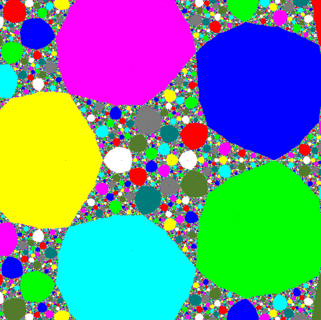
Figure 3. Dynamics of a ruling-preserving 11-map on the quadric’s rulings

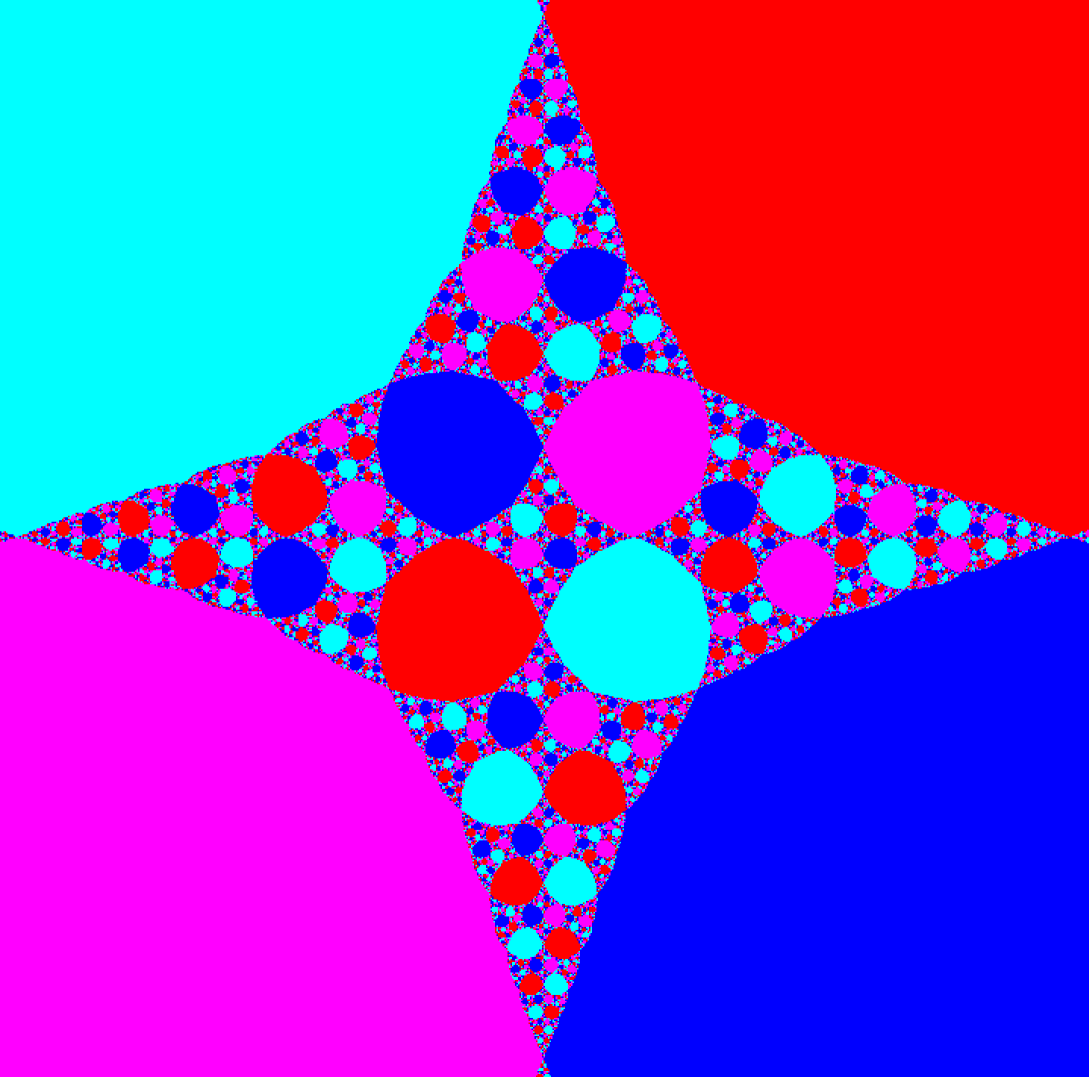
Figure 4. Four basins of attraction for the octahedral $5$-map

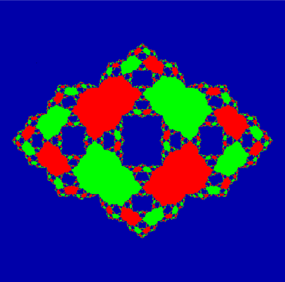
Figure 5. Three basins of attraction for $h_{11}$ restricted to a $15$-line $\mathcal{L}^{1}_{15_{ij,k\ell}}$

Figure 6. Three basins of attraction for $h_{11}$ restricted to a $30$-line $\mathcal{L}^{1}_{30_{i,jk}}$

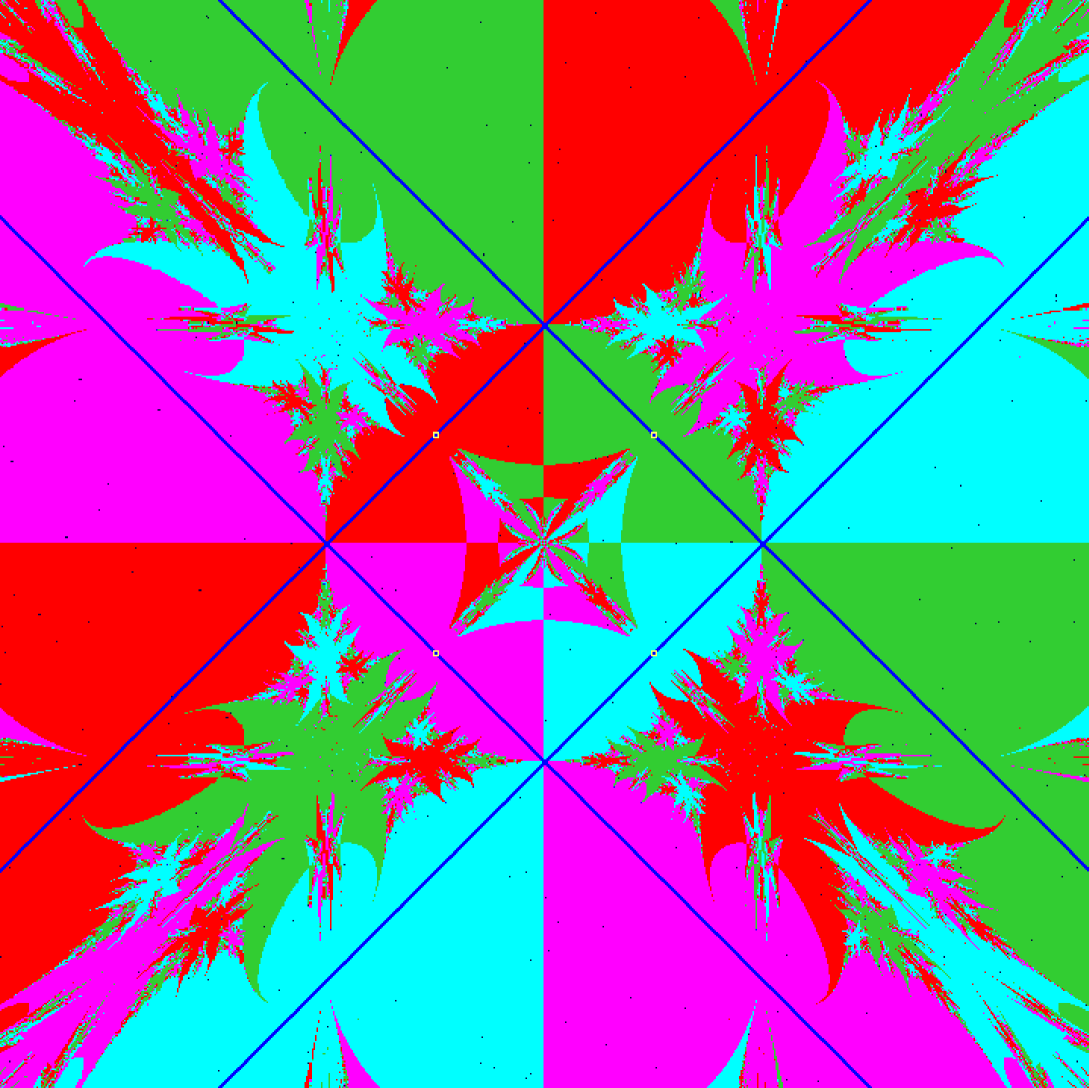
Figure 7. Chaotic attractors for $h_{11}$ on an $\mathbf{RP}^{2}$ with $\mathcal{S}_{4}$ symmetry

Figure 8. Chaotic attractor for $h_{11}$ on an $\mathbf{RP}^{2}$ with $\mathcal{S}_{3}$ symmetry

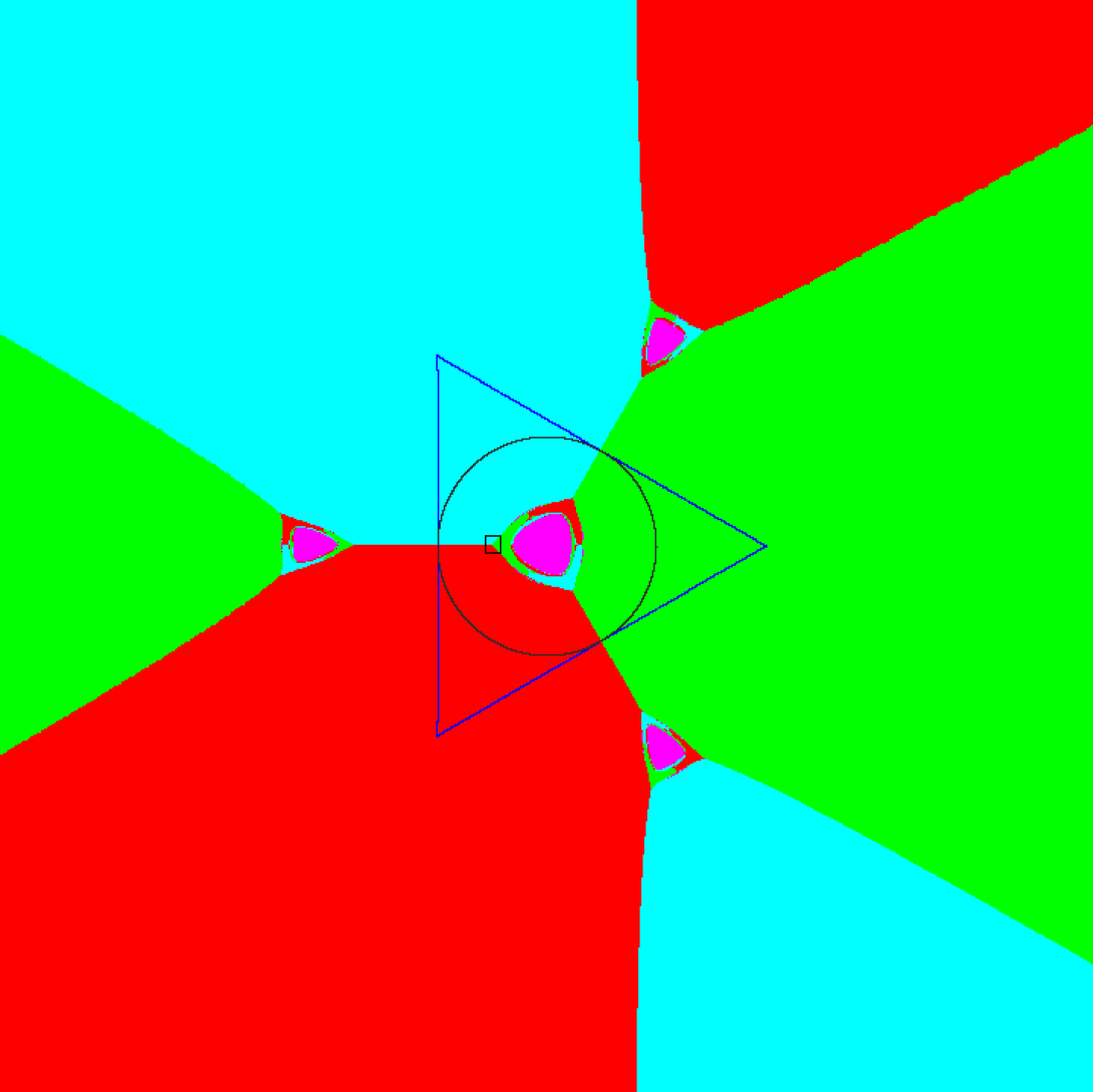
Figure 9. Four basins of attraction for $f_{6}$ restricted to an $\mathbf{RP}^{2}$

Figure 10. Critical set of $f_{6}$ restricted to an $\mathbf{RP}^{2}$

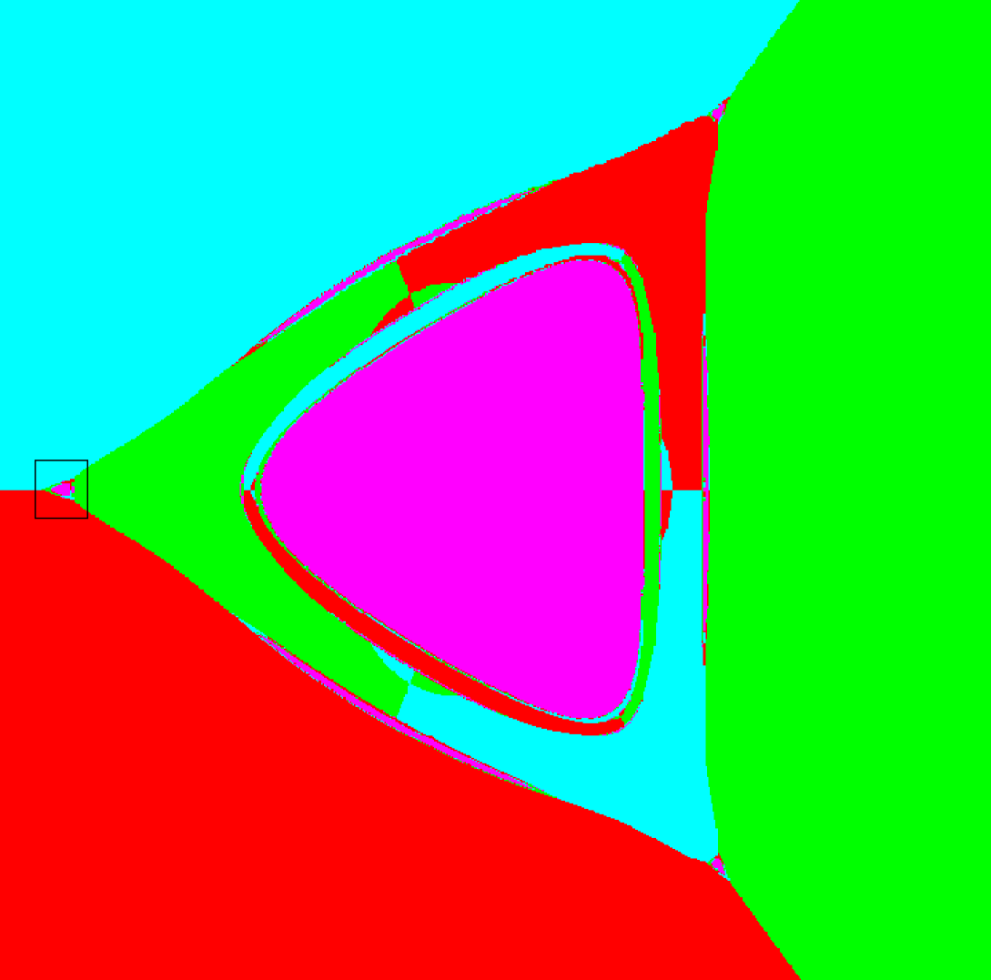
Figure 11. Detail of the left cusp of central basins in Figure 9

Figure 12. Detail of the left cusp in Figure 11

Figure 13. Three basins of attraction for $f_{6}$ restricted to a $15$-line $\mathcal{L}^{1}_{15_{ij,k\ell}}$

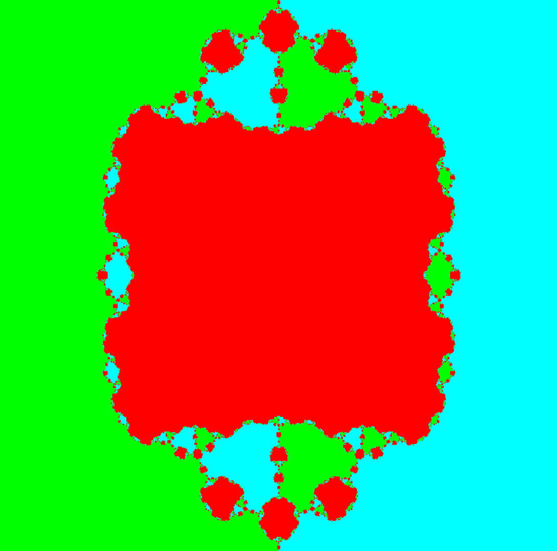
Figure 14. Magnified view of the boxed region in Figure 13

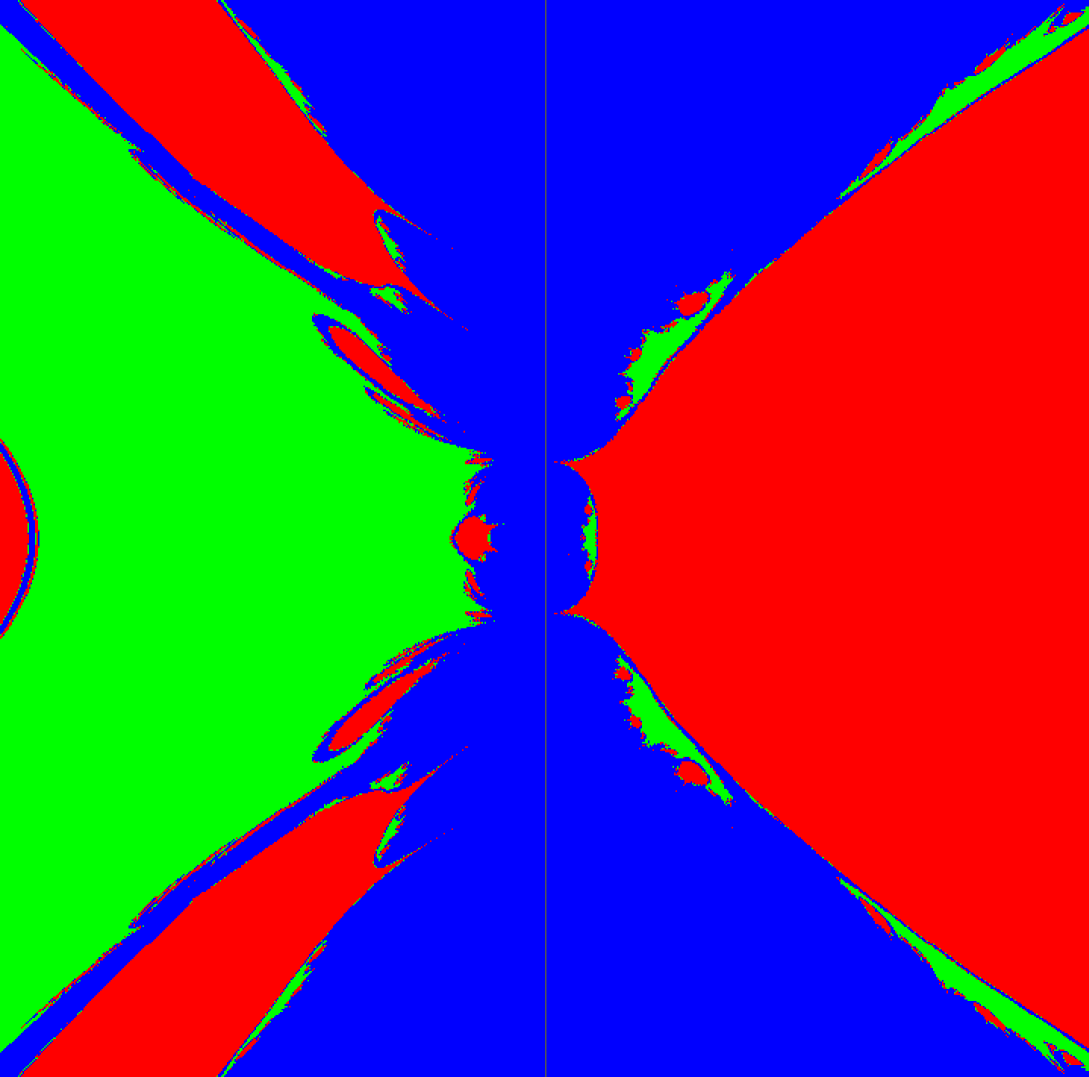
Figure 15. Chaotic attractor for $f_{6}$ on an $\mathbf{RP}^{2}$ with $\mathbf{Z}_{2}\times\mathbf{Z}_{2}$ symmetry

References

- [Crass forthcoming] S. Crass. Solving the sextic by iteration: A study in complex geometry and dynamics. To appear in Experiment. Math.
- [Crass 1999a] S. Crass, 1999. Mathematica notebook and data files that implement the quintic-solving algorithm based on the dynamics of . See www.buffalostate.edu/ crasssw.
- [Crass 1999b] S. Crass, 1999. “Solving the quintic by iteration in three dimensions.” Preprint at xxx.lanl.gov/abs/math.DS/9903054.
- [Crass 1999c] S. Crass, 1999. “Solving the octic by iteration in six dimensions.” Preprint at xxx.lanl.gov/abs/math.DS/.
- [Doyle and McMullen 1989] P. Doyle and C. McMullen. Solving the quintic by iteration. Acta Math. 163 (1989), 151-80.
- [Hodge and Pedoe 1968] W. Hodge and D. Pedoe. Methods of Algebraic Geometry. Cambridge University Press, 1968.
- [Klein 1956] F. Klein. Lectures on the Icosahedron and the Solutions of Equations of the Fifth Degree. Translated by G. Morrice. Dover, 1956.
- [Nusse and Yorke 1998] H. Nusse and J. Yorke. Dynamics: Numerical Explorations, 2e Springer-Verlag, 1998. Computer program Dynamics 2 by B. Hunt and E. Kostelich.
- [Orlik and Terao 1992] P. Orlik and H. Terao. Arrangements of Hyperplanes. Springer-Verlag, 1992.
- [Shephard and Todd 1954] G.C. Shephard and T.A. Todd. Finite unitary reflection groups. Canad. J. Math. 6 (1954), 274-304.