Finite groups, spherical 2-categories, and 4-manifold invariants

Abstract

In this paper we define a class of state-sum invariants of closed oriented piece-wise linear 4-manifolds using finite groups. The definition of these state-sums follows from the general abstract construction of 4-manifold invariants using spherical 2-categories, as we defined in an earlier paper. We show that the state-sum invariants of Birmingham and Rakowski, who studied Dijkgraaf-Witten type invariants in dimension 4, are special examples of the general construction that we present in this paper. They showed that their invariants are non-trivial by some explicit computations, so our construction includes interesting examples already. Finally, we indicate how our construction is related to homotopy 3-types. This connection suggests that there are many more interesting examples of our construction to be found in the work on homotopy 3-types, by Brown, for example.

1 Introduction

In [37] we defined spherical 2-categories and showed how to construct state-sum invariants of closed oriented PL 4-manifolds with them. Roughly speaking spherical 2-categories are monoidal 2-categories with duals, as defined by Baez and Langford [6, 7], such that the categorical trace satisfies a small set of conditions. The main point in that paper was to find a construction that would generalize Crane and Frenkel’s construction [23], which uses involutory Hopf categories, and Crane and Yetter’s construction  [24, 25], which uses tortile categories. Let us exlain this in some detail.

In [23] Crane and Frenkel sketched a general approach to the construction of 4D TQFT’s. At its core is the so-called categorical ladder, as shown in Fig. 1.

Figure 1: The categorical ladder

For an explanation of this diagram see [23]. Here we only explain the diagonal going from algebra to monoidal 2-category. In [32] the authors show that any finite dimensional semi-simple associative algebra, $A$, can be used for the construction of state-sum invariants of 2-manifolds (surfaces). This is not the place to recall the construction in detail. What is of interest to us in this introduction is the main idea behind the construction, which accounts for the invariance of the state-sums. To show that the value of a state-sum of a triangulated surface does not depend on the chosen triangulation, so that this value is a topological invariant of the surface, one has to prove that the value does not change under any of the 2D Pachner moves. The $n$-dimensional Pachner moves express the combinatorial equivalence relation between triangulations of two PL homeomorphic closed oriented PL $n$-manifolds. More precisely, two triangulated $n$-manifolds, $(M_{1},{\cal T}_{1})$ and $(M_{2},{\cal T}_{2})$, are PL homeomorphic if and only if there exists a finite sequence of $n$-dimensional Pachner moves which transform ${\cal T}_{1}$ into a new, but PL-homeomorphic, triangulation of $M_{1}$ which is isomorphic to ${\cal T}_{2}$ as a simplicial complex. In dimension 2 the Pachner moves are the ones depicted in Fig. 2 and Fig. 3.

Figure 2: $2\rightleftharpoons 2$ Pachner move

Figure 3: $1\rightleftharpoons 3$ Pachner move

As shown in Fig. 4 the $2\rightleftharpoons 2$ move can be interpreted as a diagrammatic way of expressing the associativity of $A$, if one labels the edges with elements of $A$.

Figure 4: $2\rightleftharpoons 2$ Pachner move

For the partition function of the state-sum of a triangulated surface $(S,{\cal T})$ one has to label the edges of $\cal T$ with basis elements of $A$ and associate to each triangle the multiplication constant of $A$ determined by the three labels on the edges in the boundary of the triangle. Therefore, Fig. 4 shows that invariance of the state-sum under the $2\rightleftharpoons 2$ Pachner move follows from the equations satisfied by the multiplication constants expressing the associativity of $A$. Invariance under the other 2D move is a bit trickier and involves the semi-simplicity of $A$ as well. Since we are only interested in the foundational ideas in this introduction, we do not explain the invariance under this move.

In dimension 3 there are two different constructions of state-sum invariants. One is due to Kuperberg [36], who uses finite dimensional involutory Hopf algebras as algebraic input. In [22] the reader can find a detailed account of Kuperberg’s invariants, which we do not reproduce. The other construction in dimension 3 is due to Turaev and Viro [47]. Several authors [11, 46, 50] generalized Turaev and Viro’s original construction, which uses a non-degenerate quotient of the monoidal category of finite dimensional representations of $U_{q}(sl(2))$, the quantum group corresponding to the Lie algebra $sl(2)$, for certain roots of unity $q$, and axiomatized the categorical input that is needed. The most “economical” axiomatization is due to Barrett and Westbury. They defined the notion of a spherical category, which is a monoidal category with duals satisfying some extra conditions. The relation with Kuperberg’s work was made explicit by Barrett and Westbury [10]: the monoidal category of finite dimensional representations of a finite dimensional involutory Hopf algebra, $H$, is a particular kind of spherical category, $C_{H}$, and Kuperberg’s invariants using $H$ are equal to Barrett and Westbury’s invariants using $C_{H}$. However, there are many spherical categories whose objects are not representations of involutory Hopf algebras, and some of these give very interesting invariants, such as the Turaev-Viro invariants.

Without recalling the details of Barrett and Westbury’s construction, let us explain how this construction of 3D state-sums can be understood in the light of the former construction of 2D state-sums. We already remarked that the invariance of the 2D state-sums is mainly due to the deep correspondence between the combinatorics of the 2D Pachner moves and the algebraic equation corresponding to the associativity of algebras. In 3D we have replaced the algebra by a monoidal category, which has one extra layer of structure formed by the morphisms. The associativity in the algebra, which is an equation, is therefore replaced by the so called associator in the monoidal category, which is a natural isomorphism instead of an equation. It is well known that the associator of a monoidal category has to satisfy a coherence relation, corresponding to the Stasheff pentagon diagram:

$$\begin{CD}X(Y(WZ))@>{}>{}>(XY)(WZ)@>{}>{}>((XY)W)Z\\ @V{}V{}V&&@A{}A{}A\\ X((YW)Z)&@>{}>{}>&(X(YW))Z\end{CD}.$$

In this diagram we have written $XY$ as a shorthand for $X\otimes Y$, and the arrows indicate the use of the associator. For the pentagon diagram to be commutative the composite of the two instances of the associator over the top of the diagram has to be equal to the composite of the three instances of the associator around the bottom. Thus, in going from 2D to 3D, the elements of an algebra are replaced by the objects in a monoidal category and the associativity equation is replaced by the associativity isomorphism which satisfies a new equation of its own. This “replacement process” was called categorification by Crane and Frenkel [23]. There Remains the question, what the pentagon equation of the associator has to do with the invariance of the 3D state-sums. The most satisfactory answer to this question, at least in the opinion of the author of this article, is obtained by a close analysis of the 3D Pachner moves. These moves can be seen in Figs. 5, 6.

Figure 5: $2\rightleftharpoons 3$ Pachner move

Figure 6: $1\rightleftharpoons 4$ Pachner move

In order to understand the invariance of the state-sums one would like to see the diagrammatic analogue of categorification and its relation with the Stasheff pentagon. This diagrammatic interpretation of categorification is due to Carter, Kauffman and Saito [20]. A little thought shows what it should look like: the “diagrammatic equations” expressing the 2D Pachner moves should be considered as “diagrammatic isomorphisms”, whatever that may be, and a 3D Pachner move should be interpreted as a diagrammatic equation between two finite sequences of these isomorphisms. It turns out that a diagrammatic isomorphism should be understood as the gluing of the source and target of the isomorphism. The reason for this is that any $n$-dimensional Pachner move corresponds to a partition of the boundary of an $n+1$-simplex into two connected parts which share a common boundary. Thus, replacing the diagrammatic equation that corresponds to an $n$-dimensional Pachner move by a diagrammatic isomorphism can be interpreted as gluing the two $n$-dimensional simplicial complexes, which define the two sides of the move, along their common boundary and filling up the missing $n+1$-cell in order to obtain the whole $n+1$-simplex. This $n+1$-simplex can never be part of the triangulation of an $n$-manifold, which is why the $n$D Pachner moves have to be equations in dimension $n$, whereas in the triangulation of an $n+1$-manifold there is enough space, so the $n$D Pachner moves can no longer hold as equations in dimension $n+1$. In order to illustrate this, we have copied Fig. 7 from [20], with permission from the authors, which shows how the $2\rightleftharpoons 3$ Pachner move in 3D can be seen as an equation between two finite sequences of 2D Pachner move.

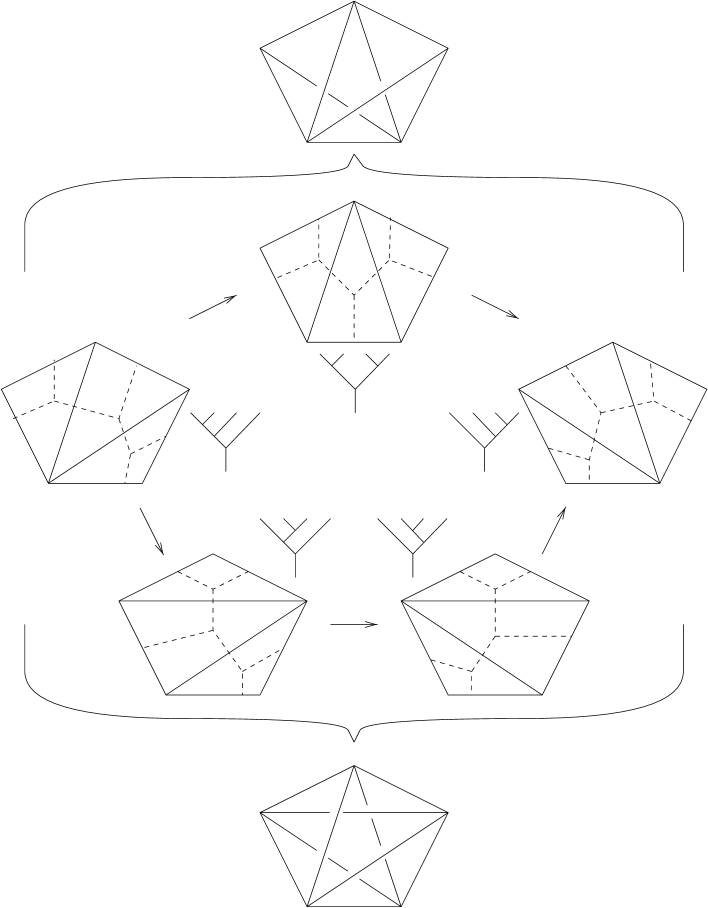
Figure 7: The pentagon and the $2\rightleftharpoons 3$ Pachner move

The arrows indicate the gluings which represent the diagrammatic isomorphisms, each of which corresponds to a 2D Pachner move, i.e., a tetrahedron. Notice the diagrammatic similarity with the Stasheff pentagon! The deep reason why the values of the Turaev-Viro type state-sums of 3-manifolds are independent of the choice of triangulation can now be expressed by saying that the algebraic categorification, which is obtained by introducing an associator which satisfies the pentagon equation, and the diagrammatic categorification, which is obtained by introducing diagrammatic isomorphisms corresponding to the 2D Pachner moves which have to satisfy the equations corresponding to the 3D Pachner moves, are somehow equivalent. Of course this remark is rather vague and the author of this article does not know how to make it into a mathematically rigorous statement. The problem is to understand the exact relation between the coherence relations in (weak) $n$-categories and the $n$-dimensional Pachner moves. Unfortunately there are several definitions of weak $n$-categories by now, and no one knows whether they are “equivalent” in some sense. One difference between the various approaches lies in the shape of the diagrams that represent the $k$-morphisms for $2\leq k\leq n$; see [2] for a nice review of the different approaches. The work of Tamsamani [44], who defines weak $n$-categories via a simplicial approach, might shed some light on the relation between coherence relations and Pachner moves one day. Although not mathematically rigorous, we hope that the arguments sketched above convince the reader that the invariance of Barrett and Westbury’s state-sums using spherical categories is no miracle. The same arguments also indicate how to proceed in dimension 4.

The deep insight in Crane and Frenkel’s paper is that the categorification of the 2D state-sums yields the 3D state-sums, and that the invariance of the latter are a consequence of the invariance of the former and the general principle of categorification. Since they were interested in the construction of 4D state-sums, they were led to study the categorification of the 3D state-sums. By the arguments above, however vague they may seem, the invariance of the 3D state-sums should guarantee the invariance of their categorifications. Crane and Frenkel chose to categorify Kuperberg’s construction, which led them to the definition of an involutory Hopf category. This is a monoidal category with a comonoidal structure satisfying the axioms of a Hopf algebra up to natural isomorphisms, which satisfy a new set of equations themselves. The problem is that their categorification inherited Kuperberg’s severe restriction of the Hopf algebra having to be involutory. As is well known, the most interesting 3D invariants are related to the quantum groups, which are not involutory. In their conclusions Crane and Frenkel conjecture the possibility of categorifying the Turaev-Viro type constructions, which would lead to a more general construction, just as Barrett and Westbury’s construction is more general than Kuperberg’s. Crane and Frenkel mention that the representations of a Hopf category are categories with a categorified module structure, as defined by Kapranov and Voevodksy [35], and that these should form a monoidal 2-category. Neuchl [39] studied the monoidal 2-categories of representations of Hopf categories in his PhD dissertation. In [37] the author of the present article studied the categorification of Barrett and Westbury’s construction and defined spherical 2-categories and the corresponding 4D state-sum invariants.

In going from 2D to 3D we had to replace the concept of algebra by that of monoidal category, thus allowing for one more layer of structure. Analogously, in going from 3D to 4D, we have to add one more layer: besides objects and morphisms, we want morphisms between morphisms, which are called 2-morphisms. Structures of this sort, called bicategories, were defined by Benabou [13]. He also showed that a 2-category with one object, $X$, can be considered as a monoidal category whose objects are the endomorphisms on $X$ and whose morphisms are the 2-morphisms between these endomorphisms. The tensor product is defined by the composition of the endomorphisms. Note that in a bicategory the composition of (1-)morphisms need not to be strictly associative: in general there is a non-trivial associator which satisfies the pentagon equation. Bicategories are not as exotic as may seem at first. Two good examples are the following: the bicategory of all (small) categories and the fundamental 2-groupoid of a topological space. The objects of the former are all (small) categories, the 1-morphisms are all functors between categories, and the 2-morphisms are all natural transformations between the functors. In the second example, the objects are the points in the space, the 1-morphisms are the paths between points, and the 2-morphisms are “homotopy classes” of homotopies between paths. Note that in the first example the composition of the 1-morphisms is strictly associative, whereas in the second example it is not. Monoidal 2-categories were systematically studied by Kapranov and Voevodsky [35], although some other authors had studied particular cases before them. To explain the notion of monoidal 2-category would take us too far from our main line of reasoning in this introduction. Suffice it to mention one important aspect of it, which, hopefully, was expected by the reader after reading the earlier paragraphs: the associator which controls the lack of associativity of the tensor product does not satisfy the pentagon equation “on the nose”. Instead there is a modification, i.e., a natural 2-isomorphism, between the two sides of the pentagon equation, called the pentagonator. This pentagonator is required to satisfy a new equation, which is sometimes called the non-abelian 4-cocycle relation. This is completely in conformity with the “basic rule” of categorification: equations which hold on the nose in dimension $n$ are to be substituted by isomorphisms in dimension $n+1$ which are required to satisfy new equations.

For the proof of invariance of the 4D state-sums which we defined in [37] it is necessary to express the 4D Pachner moves as “categorifications” of the 3D Pachner moves, which we show in Figs. 8, 9, 10. Again, these figures have been copied from [20]

Figure 8: $3\rightleftharpoons 3$ Pachner move

Figure 9: $2\rightleftharpoons 4$ Pachner move

Figure 10: $1\rightleftharpoons 5$ Pachner move

Recall that the 3D Pachner moves correspond to partitions of the boundary of a 4-simplex into two connected parts with a common boundary. Therefore, each arrow in the diagrams of the 4D Pachner moves corresponds to the gluing of the two parts of the boundary of a 4-simplex corresponding to a 3D Pachner move, after which there is only one way to fill up the missing 3-cell. In this way one side of a diagram builds up one connected part of the boundary of a 5-simplex, whereas the other side builds up the complementary part of that boundary.

In this article we study a particular class of spherical 2-categories and the corresponding state-sums. Since in this case the partition function is relatively simple, one can prove independence directly, which is what we do in Sect. 4. Let us just mention that, as in going from 2D to 3D, the algebraic categorification and the “topological categorification” go hand in hand, which “explains” the invariance of our state-sums.

Conjecturally [37] the representations of an involutory Hopf category, $H$, form a spherical 2-category, $C_{H}$. Bearing Barrett and Westbury’s results [10] in mind we conjecture that the Crane-Frenkel invariants using $H$ are equal to our invariants using $C_{H}$. Furthermore, we proved in [37] that a spherical 2-category with one object is nothing but a tortile category, which is the kind of category that Crane and Yetter [24, 25] used for their construction of 4-manifold invariants. But for a small technical detail, which we explain in Sect. 2, it is clear that our whole setup generalizes Crane and Yetter’s setup. Crane and Yetter’s invariants are a partial categorification of the Turaev-Viro type invariants. Let us finish this part of the introduction by noting that our story about categorification is far from complete. We apologize to everyone whose contributions to the subject we have not mentioned. In this introduction we have tried to give a comprehensive overview of the results that lead to our own work, rather than a review of the whole subject. For a more complete picture see [4].

We summarize our results. For the rest of this paper, let $G$ be any finite group, $H$ any finite abelian group, $R$ any commutative ring with unit and involution, which is denoted by $*$, and $R^{*}$ its group of invertible elements. If $r$ is an element in $R$, we call $r^{*}$ its conjugate. In Section 2 we define $\mathbb{N}(G,H,R)$. Roughly speaking this is the 2-category of which the objects are finite linear combinations of elements of $G$ with non-negative integer coefficients, the 1-endomorphisms of an object $g\in G$ are finite linear combinations of elements of $H$ with non-negative integer coefficients, and the 2-endomorphisms of a 1-endormorphism $h\in H$ are elements of the ring $R$. Composition on all levels is induced by the group operations, which we write multiplicatively throughout this paper.

In Section 3 we define the kind of monoidal structure on $\mathbb{N}(G,H,R)$ that we are interested in. We also define an equivalence relation on the set of monoidal structures.

In Section 4 we define our state-sum and indicate how we derived its definition from our construction in [37]. We do not repeat that abstract construction here, because it would increase the number of pages considerably and might confuse the less category-minded reader. We prove invariance of the state-sums that are defined in this paper directly, without going back to the abstract results in [37]. For a thorough understanding of the results in this paper it is probably better to read [37] anyway, but formally the results in this paper are self-contained. It is interesting to note that our construction yields the “twisted” version of Yetter’s [49] construction for the case of 2-simple path-connected homotopy 2-types. A 2-simple path-connected space $E$ is a path-connected space for which the action of $\pi_{1}(E)$, the fundamental group, is trivial on $\pi_{2}(E)$, the second homotopy group. Yetter gives a construction of state-sums for arbitrary homotopy 2-types, or “categorical groups”, which is equivalent.

In Section 5 we relate our results to the theory of homotopy 3-types in the form of Postnikov systems. This interpretation in terms of Postnikov systems provides a nice link with Freed and Quinn’s work in [31, 41, 42].

2 ${\mathbb{N}}(G,H,R)$

In this section we define the semi-strict monoidal 2-category ${\mathbb{N}}(G,H,R)$. We recall that Kapranov and Voevodsky [35] defined the more general notion of a weak monoidal 2-category, and that Gordon, Power and Street [33] showed that any weak monoidal 2-category is equivalent, in an apropriate sense, to a semi-strict monoidal 2-category. As a matter of fact they proved a more general strictification theorem about weak 3-categories, or tricategories, but we only need the case of a tricategory with one object which corresponds to a weak monoidal 2-category by reindexing of the $k$-morphisms for $0\leq k\leq 3$.

First let us define the category ${\mathbb{N}}(H,R)$.

Definition 2.1

${\mathbb{N}}(H,R)$ is the $R$-linear finitely semi-simple category with the simple objects being precisely the elements of $H$, and for which the $R$-module of endomorphisms of an object $h\in H$ is defined by $\hbox{End}(h)=R$. The composite of two such endomorphisms, $r_{1}$ and $r_{2}$, is defined by their product $r_{1}r_{2}$ in $R$.

Note that the objects of ${\mathbb{N}}(H,R)$ are just finite linear combinations of elements of $H$ with non-negative integer coefficients. Another way of saying this is that the objects are just the elements of the so called group rig [27], ${\mathbb{N}}(H)$. If we choose an ordering on the elements of $H$, we can represent the morphisms by matrices. Let us explain this in a little more detail. Suppose $H$ has order $k$. We define the degree of a finite linear combination of elements of a group with non-negative integer coefficients as the sum of the coefficients. We denote the degree of such a linear combination $X$ by $\hbox{deg}(X)$. A morphism with source $X=n_{1}h_{1}+\cdots+n_{k}h_{k}$ and target $Y=m_{1}h_{1}+\cdots+m_{k}h_{k}$ can be represented by a $\hbox{deg}(X)\times\hbox{deg}(Y)$ block diagonal matrix with coefficients in $R$. The $i$-th block has size $n_{i}\times m_{i}$. Composition is defined by matrix multiplication. The product in $H$ induces a monoidal structure on ${\mathbb{N}}(H,R)$. Note that we can take ${\mathbb{N}}(H,R)$ to be symmetric, since $H$ is abelian, so $h_{1}h_{2}=h_{2}h_{1}$. There is also a left duality on ${\mathbb{N}}(H,R)$: the left dual of an element $X=n_{1}h_{1}+\cdots+n_{k}h_{k}$ is defined by $X^{*}=n_{1}h_{1}^{-1}+\cdots n_{k}h_{k}^{-1}$. The dual of a morphism, represented by a matrix, is defined by the conjugate transpose of that matrix. It is not hard to check that this symmetry and this duality define a ribbon structure on ${\mathbb{N}}(H,R)$.

We are now ready to define the strict 2-category ${\mathbb{N}}(G,H,R)$.

Definition 2.2

${\mathbb{N}}(G,H,R)$ is the ${\mathbb{N}}(H,R)$-linear finitely semi-simple strict 2-category of which the simple objects are precisely the elements of $G$, and for which the ${\mathbb{N}}(H,R)$-module category of endomorphisms on $g\in G$ is defined by $\hbox{End}(g)={\mathbb{N}}(H,R)$.

Let us explain this definition. The objects of ${\mathbb{N}}(G,H,R)$ are elements of ${\mathbb{N}}(G)$. Choose an ordering on the elements of $G$ and $H$. We can now represent 1- and 2-morphisms by matrices. Let $l$ be the order of $G$. A 1-morphism between two objects $X=n_{1}g_{1}+\ldots+n_{l}g_{l}$ and $Y=m_{1}g_{1}+\ldots+m_{l}g_{l}$ is a $\hbox{deg}(X)\times\hbox{deg}(Y)$ block diagonal matrix, $f$, with coefficients being elements of ${\mathbb{N}}(H)$. The size of the $i$-th block is equal to $n_{i}\times m_{i}$. The composition is given by matrix multiplication, where the operations on the coefficients are the multiplication and the addition in ${\mathbb{N}}(H)$. A 2-morphism between two such 1-morphisms, $f$ and $g$, is represented by a $\hbox{deg}(X)\times\hbox{deg}(Y)$ block diagonal matrix, $(\alpha^{i}_{j})$, where the coefficient $\alpha^{i}_{j}$ is a $\hbox{deg}(f^{i}_{j})\times\hbox{deg}(g^{i}_{j})$ matrix with coefficients in $R$. The horizontal composite of two 2-morphisms $\alpha$ and $\beta$, which we denote by $\alpha\circ\beta$, is defined by matrix multiplication, but the operations on the coefficients are more complicated than in the case of the 1-morphisms. We define $(\alpha\circ\beta)^{i}_{j}=\oplus_{k}(\alpha^{i}_{k}\otimes\beta^{k}_{j})$. Note that the coefficients $\alpha^{i}_{k}$ and $\beta^{k}_{j}$ are matrices themselves with coefficients in $R$. In general the tensor product of two matrices, $x$ and $y$, is defined by $(x\otimes y)^{ij}_{kl}=x^{i}_{k}y^{j}_{l}$, and the direct sum is defined by

$$x\oplus y=\begin{pmatrix}x&0\\ 0&y\end{pmatrix}.$$

The vertical composite of two 2-morphisms, $\alpha$ and $\beta$, which we denote by $\alpha\cdot\beta$, is defined by coefficientwise multiplication, i.e., $(\alpha\cdot\beta)^{i}_{j}=\alpha^{i}_{j}\beta^{i}_{j}$. Note that, just as in the completely coordinatized version of the monoidal 2-category of 2-vector spaces, $2\hbox{Vect}_{cc}$, defined by Kapranov and Voevodsky [35], the coefficients of the 2-morphisms are matrices themselves, so their multiplication is given by matrix multiplication. Note also that this multiplication is well defined for any pair of composable 2-morphisms: for any $\alpha\colon f\to g$ and $\beta\colon g\to h$, the matrix $\alpha^{i}_{j}$ has size $f^{i}_{j}\times g^{i}_{j}$ and $\beta^{i}_{j}$ has size $g^{i}_{j}\times h^{i}_{j}$. As always, we write the composites of 1- and 2-morphisms in the diagrammatic order. It is easy to check that all compositions are strictly associative.

The semi-strict monoidal structure on ${\mathbb{N}}(G,H,R)$ is induced by the multiplication in $G$, $H$, and $R$. For any two objects $X$ and $Y$, we define $X\otimes Y=XY$. For any 1-morphism $f$ and any object $Y$ we define $f\otimes Y=f\otimes 1_{Y}$, where $1_{Y}$ is the identity on $Y$. In terms of coefficients this becomes $(f\otimes 1_{Y})^{ij}_{kl}=f^{i}_{k}\delta^{j}_{l}$, with $\delta$ being the Kronecker delta. For any 2-morphism $\alpha$ and any object $Y$, we define $\alpha\otimes Y=\alpha\otimes 1_{1_{Y}}$, where $1_{1_{Y}}$ is the identity 2-morphism of the identity 1-morphism on $Y$. In terms of coefficients this becomes $(\alpha\times 1_{1_{Y}})^{ij}_{kl}=\alpha^{i}_{k}\otimes(1_{Y})^{j}_{l}$. Note that $\alpha$ and $1_{Y}$ are matrices themselves, so that there tensor product differs from their product in general. Likewise we define $Y\otimes f$ and $Y\otimes\alpha$. It is easy to check that these tensor products are strictly associative. The tensorator

$$\bigotimes\nolimits_{f,g}\colon(f\otimes Y)(X^{\prime}\otimes g)\Rightarrow(X\otimes g)(f\otimes Y^{\prime})$$

of two 1-morphisms $f\colon X\to X^{\prime}$ and $g\colon Y\to Y^{\prime}$ is defined by the operator that interchanges the two tensor factors. Concretely, we have

$$[(f\otimes Y)(X^{\prime}\otimes g)]^{ij}_{kl}=f^{i}_{k}g^{j}_{l}$$

and

$$[(X\otimes g)(f\otimes Y^{\prime})]^{ij}_{kl}=g^{i}_{k}f^{j}_{l},$$

so the tensorator becomes

$$(\bigotimes\nolimits_{f,g})^{ij}_{kl}=P_{f^{i}_{k}g^{j}_{l}},$$

where $P_{f^{i}_{k}g^{j}_{l}}$ is the $\hbox{deg}(f^{i}_{k})\times\hbox{deg}(g^{j}_{l})$ matrix with coefficients $(P_{f^{i}_{k}g^{j}_{l}})^{mn}_{rs}=\delta^{m}_{s}\delta^{n}_{r}$. This defines a semi-strict monoidal structure on ${\mathbb{N}}(G,H,R)$. We remark that ${\mathbb{N}}(G,\{1\},{\mathbb{C}})$ is equal to $2\hbox{Hilb}[G]$, which we defined in [37]. If $G=\{1\}$ also, then we recover the definition of the completely coordinatized version of the monoidal 2-category of 2-vector spaces, $2\hbox{Vect}_{cc}$, see [35].

We can now define the left-duality on ${\mathbb{N}}(G,H,R)$ in terms of matrices. The dual of an object $X=n_{1}g_{1}+\cdots+n_{l}g_{l}$ is defined by $X^{*}=n_{1}g^{-1}+\cdots+n_{l}g^{-1}$. The dual of a 1-morphism, represented by a matrix $f$, is defined by the transpose of $f$ with dual coefficients. Recall that the dual of a coefficient $m_{1}y_{1}+\cdots+m_{k}h_{k}$ is defined by $m_{1}h_{1}^{-1}+\cdots m_{k}h_{k}^{-1}$. The dual of a 2-morphism, $\alpha$, is defined by the matrix $\alpha^{*}$, where $(\alpha^{*})^{i}_{j}$ is the conjugate transpose of $\alpha^{i}_{j}$. This definition of the duality the author derived from the definition of duality in the monoidal 2-category of 2-Hilbert spaces by Baez [1]. Baez defined a “weak” version of 2-Hilbert spaces, the underlying monoidal 2-category of which is equivalent to $2\hbox{Vect}$, the non-coordinatized version of 2-vector spaces [35]. For our application it is better to work with the completely coordinatized version, $2\hbox{Hilb}_{cc}$, which is semi-strict [37]. Just as for $2\hbox{Hilb}_{cc}$, it is not hard to show that this duality satisfies the spherical conditions [37]. We do not prove this, because we do not need it explicitly in this article.

3 Monoidal structures on ${\mathbb{N}}(G,H,R)$

The most interesting state-sums are related to weakenings of the semi-strict monoidal structure on ${\mathbb{N}}(G,H,R)$. These weakenings can be defined, essentially, by following the definition of a monoidal 2-category by Kapranov and Voevodsky [35]. We repeat that Kapranov and Voevodsky’s definition coincides with that of Gordon, Power and Street’s [33] definition of a tricategory with one object. Kapranov and Voevodsky, using MacLane and Pare’s coherence theorem [38], assume that the underlying 2-category is strict. We do not want to make this assumption, because it is too restrictive for our purpose. Therefore we have to keep in account the non-associativity of the composition of the edges in the diagrams in [35]. We assume that this non-associativity is controlled by a coherent associator, so it does not matter how we choose to parenthesize the boundary 1-morphisms in the diagrams. We just make one choice and work out the diagrams. Any other choice will lead to equivalent diagrams. Before going on, let us have a look at this associator. Note that we can restrict our attention to the 1-morphisms in $\hbox{End}(1)$, because the general case then follows by linearity. An associator on 1-morphisms in $\hbox{End}(1)$ is a family of 2-isomorphisms

$$\alpha^{1}_{h_{1},h_{2},h_{3}}\colon h_{1}(h_{2}h_{3})\Rightarrow(h_{1}h_{2})h_{3},$$

indexed by triples of 1-morphisms. Since all 1-morphisms are sums of simple 1-morphisms, which are simply elements of $H$ in this case, we only have to define $\alpha^{1}$ on triples of simple 1-morphisms; the general definition then follows by extending $\alpha^{1}$ linearly. Note that $h_{1}(h_{2}h_{3})$ and $(h_{1}h_{2})h_{3}$ are the same 1-morphism. The associator is a natural isomorphism between the two functors $\hbox{End}(1)\times\hbox{End}(1)\times\hbox{End}(1)\to\hbox{End}(1)$ which define the two different ways of composing three 1-morphisms, indicated by the different bracketings. Hence $\alpha^{1}_{h_{1},h_{2},h_{3}}$ is just a 2-automorphism on $h_{1}h_{2}h_{3}$, i.e., an element of $R^{*}$. Thus we can define $\alpha^{1}$ as a function $H\times H\times H\to R^{*}$. As usual in category theory, we have to impose a condition on $\alpha^{1}$, called a coherence relation, in order to maintain control over the bracketing. There are five different ways of composing four 1-morphisms, and two different ways of rebracketing the composite going from right-to-left bracketing to left-to-right bracketing. This leads to the pentagon diagram which we showed in the introduction and which we repeat here.

$$\begin{CD}f(g(hj))@>{\alpha^{1}_{f,g,hj}}>{}>(fg)(hj)@>{\alpha^{1}_{fg,h,j}}>{}>((fg)h)j\\ @V{\alpha^{1}_{g,h,j}}V{}V&&@A{}A{\alpha^{1}_{f,g,h}}A\\ f((gh)j)&@>{\alpha^{1}_{f,gh,j}}>{}>&(f(gh))j\end{CD}$$

MacLane and Pare’s coherence theorem [38] implies that, if we require the pentagon diagram to be commutative, that any two strings of $\alpha^{1}$’s, i.e., composites of an arbitrary number of associators, with the same source and target are equal. This means, for example, that two different algorithms that rebracket composites of 1-morphisms will always end up using the same 2-isomorphism, although one algorithm may use a different decomposition of this 2-isomorphism than the other. This is why we impose the condition

$$\alpha^{1}_{h_{2},h_{3},h_{4}}(\alpha^{1}_{h_{1}h_{2},h_{3},h_{4}})^{-1}\alpha^{1}_{h_{1},h_{2}h_{3},h_{4}}(\alpha^{1}_{h_{1},h_{2},h_{3}h_{4}})^{-1}\alpha^{1}_{h_{1},h_{2},h_{3}}=1,$$

on $\alpha^{1}$. The maps and conditions in Def. 3.1 are obtained from Kapranov and Voevodsky’s diagrams in a similar way. In the following definition we use their hieroglyphic notation to indicate these diagrams.

Definition 3.1

A semi-weak monoidal 2-category structure on ${\mathbb{N}}(G,H,R)$ consists of the following maps:

0-associator

$\alpha^{0}\colon G\times G\times G\to H$, which corresponds to a family of simple invertible 1-morphisms $\alpha^{0}_{g_{1},g_{2},g_{3}}\colon g_{1}(g_{2}g_{3})\to(g_{1}g_{2})g_{3}$.

pentagonator

$\pi\colon G\times G\times G\times G\to R^{*}$, which corresponds to a family of invertible 2-morphisms

$$\begin{CD}g_{1}(g_{2}(g_{3}g_{4}))@>{\alpha^{0}_{g_{1},g_{2},g_{3}g_{4}}}>{}>(g_{1}g_{2})(g_{3}g_{4})@>{\alpha^{0}_{g_{1}g_{2},g_{3},g_{4}}}>{}>((g_{1}g_{2})g_{3})g_{4}\\ @V{\alpha^{0}_{g_{2},g_{3},g_{4}}}V{}V\Big{\Downarrow}\pi_{g_{1},g_{2},g_{3},g_{4}}&&@A{}A{\alpha^{0}_{g_{1},g_{2},g_{3}}}A\\ g_{1}((g_{2}g_{3})g_{4})&@>{\alpha^{0}_{g_{1},g_{2}g_{3},g_{4}}}>{}>&(g_{1}(g_{2}g_{3}))g_{4}\end{CD}$$

1-associator

$\alpha^{1}\colon H\times H\times H\to R^{*}$, which corresponds to a family of invertible 2-morphisms $\alpha^{1}_{h_{1},h_{2},h_{3}}\colon h_{1}(h_{2}h_{3})\Rightarrow(h_{1}h_{2})h_{3}$.

tensorator

$\tau\colon H\times H\to R^{*}$, which corresponds to a family of invertible 2-morphisms

$$\begin{CD}g_{1}g_{2}&@>{h_{1}}>{}>&g_{1}g_{2}\\ @V{h_{2}}V{}V\Big{\Downarrow}\tau_{h_{1},h_{2}}&&@V{}V{h_{2}}V\\ g_{1}g_{2}&@>{h_{1}}>{}>&g_{1}g_{2}\end{CD}$$

interchanger1

$\iota^{1}\colon H\times G\times G\to R^{*}$, which corresponds to a family of invertible 2-morphisms

$$\begin{CD}g_{1}(g_{2}g_{3})&@>{\alpha^{0}_{g_{1},g_{2},g_{3}}}>{}>&(g_{1}g_{2})g_{3}\\ @V{h_{1}}V{}V\Big{\Downarrow}\iota^{1}_{h_{1},g_{2},g_{3}}&&@V{}V{h_{1}}V\\ g_{1}(g_{2}g_{3})&@>{\alpha^{0}_{g_{1},g_{2},g_{3}}}>{}>&(g_{1}g_{2})g_{3}\end{CD}$$

interchanger2

$\iota^{2}\colon G\times H\times G\to R^{*}$, which corresponds to a family of invertible 2-morphisms

$$\begin{CD}g_{1}(g_{2}g_{3})&@>{\alpha^{0}_{g_{1},g_{2},g_{3}}}>{}>&(g_{1}g_{2})g_{3}\\ @V{h_{2}}V{}V\Big{\Downarrow}\iota^{2}_{g_{1},h_{2},g_{3}}&&@V{}V{h_{2}}V\\ g_{1}(g_{2}g_{3})&@>{\alpha^{0}_{g_{1},g_{2},g_{3}}}>{}>&(g_{1}g_{2})g_{3}\end{CD}$$

interchanger3

$\iota^{3}\colon G\times G\times H\to R^{*}$, which corresponds to a family of invertible 2-morphisms

$$\begin{CD}g_{1}(g_{2}g_{3})&@>{\alpha^{0}_{g_{1},g_{2},g_{3}}}>{}>&(g_{1}g_{2})g_{3}\\ @V{h_{3}}V{}V\Big{\Downarrow}\iota^{3}_{g_{1},g_{2},h_{3}}&&@V{}V{h_{3}}V\\ g_{1}(g_{2}g_{3})&@>{\alpha^{0}_{g_{1},g_{2},g_{3}}}>{}>&(g_{1}g_{2})g_{3}\end{CD}$$

All these maps are required to be normalized, i.e., their value is equal to $1$ whenever one of the factors of their argument is equal to $1$. Furthermore these maps are required to satisfy the following identities:

$(\bullet\otimes\bullet\otimes\bullet\otimes\bullet)$

$$\alpha^{0}_{g_{2},g_{3},g_{4}}(\alpha^{0}_{g_{1}g_{2},g_{3},g_{4}})^{-1}\alpha^{0}_{g_{1},g_{2}g_{3},g_{4}}(\alpha^{0}_{g_{1},g_{2},g_{3}g_{4}})^{-1}\alpha^{0}_{g_{1},g_{2},g_{3}}=1.$$

$(\rightarrow\rightarrow\rightarrow\rightarrow)$

$$\alpha^{1}_{h_{2},h_{3},h_{4}}(\alpha^{1}_{h_{1}h_{2},h_{3},h_{4}})^{-1}\alpha^{1}_{h_{1},h_{2}h_{3},h_{4}}(\alpha^{1}_{h_{1},h_{2},h_{3}h_{4}})^{-1}\alpha^{1}_{h_{1},h_{2},h_{3}}=1.$$

In the following identities we avoid writing $\alpha^{1}$ constantly and bracket the remaining maps with $\lceil\rceil$ following Crane and Yetter’s [26] notation. As explained in [26] this notation means that the source and target 1-morphisms are assumed to be parenthesized from left to right. The brackets denote the strings of 1-associators that are required to make the 2-morphisms composable under this assumption. The usage of these brackets is unambiguous by the coherence relation of the 1-associator, which corresponds to $(\rightarrow\rightarrow\rightarrow\rightarrow)$.

$(\bullet\otimes\bullet\otimes\bullet)$

$$\lceil\tau_{h_{1}h_{2},h_{3}}\rceil=\lceil\tau_{h_{2},h_{3}}\rceil\lceil\tau_{h_{1},h_{3}}\rceil,$$

and

$$\lceil\tau_{h_{1},h_{2}h_{3}}\rceil=\lceil\tau_{h_{1},h_{2}}\rceil\lceil\tau_{h_{1},h_{3}}\rceil.$$

$(\bullet\otimes\bullet\otimes\bullet\otimes\bullet\otimes\bullet)$

$$\lceil\pi_{g_{2},g_{3},g_{4},g_{5}}\rceil\lceil\pi_{g_{1},g_{2}g_{3},g_{4},g_{5}}\rceil\lceil\iota^{1}_{\alpha^{0}_{g_{1},g_{2},g_{3}};g_{4};g_{5}}\rceil\lceil\pi_{g_{1},g_{2},g_{3},g_{4}g_{5}}\rceil=$$

$$\lceil\iota^{2}_{g_{1};\alpha^{0}_{g_{2},g_{3},g_{4}};g_{5}}\rceil\lceil\pi_{g_{1},g_{2},g_{3},g_{4}}\rceil\lceil\pi_{g_{1},g_{2},g_{3}g_{4},g_{5}}\rceil\lceil(\iota^{3}_{g_{1};g_{2};\alpha^{0}_{g_{3},g_{4},g_{5}}})^{-1}\rceil\lceil\pi_{g_{1}g_{2},g_{3},g_{4},g_{5}}\rceil.$$

$(\rightarrow\otimes\bullet\otimes\bullet\otimes\bullet)$

$$\lceil\iota^{1}_{h,g_{2},g_{3}}\rceil\lceil\iota^{1}_{h,g_{2}g_{3},g_{4}}\rceil\lceil\tau^{-1}_{h;\alpha^{0}_{g_{2},g_{3},g_{4}}}\rceil=\lceil\iota^{1}_{h,g_{3},g_{4}}\rceil\lceil\iota^{1}_{h,g_{2},g_{3}g_{4}}\rceil.$$

$(\bullet\otimes\rightarrow\otimes\bullet\otimes\bullet)$

$$\lceil\iota^{2}_{g_{1},h,g_{3}g_{4}}\rceil=\lceil\iota^{2}_{g_{1},h,g_{3}}\rceil\lceil\iota^{2}_{g_{1},h,g_{4}}\rceil.$$

$(\bullet\otimes\bullet\otimes\rightarrow\otimes\bullet)$

$$\lceil\iota^{2}_{g_{1}g_{2},h,g_{4}}\rceil=\lceil\iota^{2}_{g_{1},h,g_{4}}\rceil\lceil\iota^{2}_{g_{2},h,g_{4}}\rceil.$$

$(\bullet\otimes\bullet\otimes\bullet\otimes\rightarrow)$

$$\lceil\tau_{\alpha^{0}_{g_{1},g_{2},g_{3}};h}\rceil\lceil\iota^{3}_{g_{1},g_{2}g_{3},h}\rceil\lceil\iota^{3}_{g_{2},g_{3},h}\rceil=\lceil\iota^{3}_{g_{1}g_{2},g_{3},h}\rceil\lceil\iota^{3}_{g_{1},g_{2},h}\rceil.$$

$(\rightarrow\rightarrow\otimes\bullet\otimes\bullet)$

$$\lceil\iota^{1}_{h_{1}h_{2},g_{2},g_{3}}\rceil=\lceil\iota^{1}_{h_{1},g_{2},g_{3}}\rceil\lceil\iota^{1}_{h_{2},g_{2},g_{3}}\rceil.$$

$(\bullet\otimes\rightarrow\rightarrow\otimes\bullet)$

$$\lceil\iota^{2}_{g_{1},h_{1}h_{2},g_{3}}\rceil=\lceil\iota^{2}_{g_{1},h_{1},g_{3}}\rceil\lceil\iota^{2}_{g_{1},h_{2},g_{3}}\rceil.$$

$(\bullet\otimes\bullet\otimes\rightarrow\rightarrow)$

$$\lceil\iota^{3}_{g_{1},g_{2},h_{1}h_{2}}\rceil=\lceil\iota^{3}_{g_{1},g_{2},h_{1}}\rceil\lceil\iota^{3}_{g_{1},g_{2},h_{2}}\rceil.$$

Let us briefly comment on these maps and relations. There is only one structural 1-morphism: the 0-associator, $\alpha^{0}$. It controls the non-associativity of the tensor product on objects and is given by a family of invertible 1-morphisms indexed by triples of objects. It suffices to define $\alpha^{0}$ on simple objects, i.e., elements of $G$. We assume in our definition that all structural 1-morphisms are simple. Therefore we define $\alpha^{0}$ to take values in $H$. It is now easy to derive the 3-cocycle condition in $(\bullet\otimes\bullet\otimes\bullet\otimes\bullet)$ from the corresponding diagram in [35]. Note that this diagram is just the pentagon diagram for objects and 1-morphisms. All other maps in Definition 3.1 are structural 2-morphisms. Since they are also assumed to be invertible, they take values in $R^{*}$. It suffices to index them by simple objects, i.e., elements in $G$, and simple 1-morphisms, i.e., elements in $H$. The list of maps and relations now follows easily from Kapranov and Voevodsky’s definitions. The pentagonator, $\pi$, controls the non-commutativity of the pentagon diagram for the 0-associator. This pentagon diagram corresponds to $(\bullet\otimes\bullet\otimes\bullet\otimes\bullet)$. As we already explained, the 1-associator, $\alpha^{1}$, controls the non-associativity of the composition of the 1-morphisms. The tensorator, $\tau$, is a weakening of the tensorator in the semi-strict monoidal structure on ${\mathbb{N}}(G,H,R)$. Finally, the interchangers, $\iota^{i}$ for $i=1,2,3$, define the pseudo-naturality of $\alpha^{0}$. All relations are coherence relations which ensure that the composites of any two strings of structural maps with the same source and target are equal. The assumption that all morphisms are simple is restrictive, but is inspired by the relation with homotopy theory, as explained in Section 5. A second reason for this assumption is that the calculations, which are not easy anyway, become much simpler under this assumption. We call these structures semi-weak, because we assume the units to be strict and the tensor product of an object with a 1- or 2-morphism to be trivial. Therefore some of the structural 1- and 2-morphisms in [35] become identities. This also explains why we have fewer coherence relations than Kapranov and Voevodsky have in [35]. Note that $(\bullet\otimes\bullet\otimes\bullet\otimes\bullet)$ and $(\rightarrow\rightarrow\rightarrow\rightarrow)$ are 3-cocycle conditions. The relations in $(\bullet\otimes\bullet\otimes\bullet)$ are called the hexagon relations and together with the 3-cocycle relation in $(\rightarrow\rightarrow\rightarrow\rightarrow)$ they define the structure of a braided monoidal category on $\hbox{End}(1)$, see [37]. The coherence cube $(\rightarrow\otimes\bullet\otimes\bullet)$ in Kapranov and Voevodsky’s paper becomes a consequence of the hexagon relations and the triviality of the tensor product of a simple object with a 1- or 2-morphism in our setup.

For this particular class of monoidal 2-categories it is easy to define when they are “equivalent”. We follow Gordon, Power and Street’s [33] definition of triequivalence of tricategories for the special case of tricategories with one object, which can be considered as weak monoidal 2-categories.

Definition 3.2

We say that two semi-weak monoidal 2-category structures on ${\mathbb{N}}(G,H,R)$, as defined in Def. 3.1, are 2-equivalent if there exist

1. Automorphisms $G\to G$, $H\to H$, and $R\to R$, which we denote by $g\mapsto\overline{g}$, $h\mapsto\overline{h}$, and $r\mapsto\overline{r}$. The first two automorphisms are required to be group automorphisms, the third one is required to be a unital ring automorphism which preserves the involution.

2. A map $\mu\colon H\times H\to R^{*}$, which corresponds to a family of invertible 2-morphisms $\mu_{h_{1},h_{2}}\colon\overline{h_{1}h_{2}}\Rightarrow\overline{h}_{1}\overline{h}_{2}$.

3. A map $\Phi\colon G\times G\to H$, which corresponds to a family of simple invertible 1-morphisms $\Phi_{g_{1},g_{2}}\colon\overline{g_{1}g_{2}}\to\overline{g}_{1}\overline{g}_{2}$.

4. A map $\phi\colon G\times G\times G\to R^{*}$, which corresponds to a family of invertible 2-morphisms

   $$\begin{CD}\overline{g_{1}(g_{2}g_{3})}@>{\Phi_{g_{1},g_{2}g_{3}}}>{}>\overline{g}_{1}(\overline{g_{2}g_{3}})@>{\Phi_{g_{2},g_{3}}}>{}>\overline{g}_{1}(\overline{g}_{2}\overline{g}_{3})\\ @V{\overline{\alpha^{0}_{g_{1},g_{2},g_{3}}}}V{}V\Big{\Uparrow}\phi_{g_{1},g_{2},g_{3}}&&@V{}V{(\alpha^{0})^{\prime}_{\overline{g}_{1},\overline{g}_{2},\overline{g}_{3}}}V\\ \overline{(g_{1}g_{2})g_{3}}@>{\Phi_{g_{1}g_{2},g_{3}}}>{}>(\overline{g_{1}g_{2}})\overline{g}_{3}@>{\Phi_{g_{1},g_{2}}}>{}>(\overline{g}_{1}\overline{g}_{2})\overline{g}_{3}\end{CD}$$

5. A map $\psi\colon H\times G\to R^{*}$, which corresponds to a family of invertible 2-morphisms

   $$\begin{CD}\overline{g_{1}g_{2}}&@>{\Phi_{g_{1},g_{2}}}>{}>&\overline{g}_{1}\overline{g}_{2}\\ @V{\overline{h}_{1}}V{}V\Big{\Downarrow}\psi_{h_{1},g_{2}}&&@V{}V{\overline{h}_{1}}V\\ \overline{g_{1}g_{2}}&@>{\Phi_{g_{1},g_{2}}}>{}>&\overline{g}_{1}\overline{g}_{2}\end{CD}$$

6. A map $\chi\colon G\times H\to R^{*}$, which corresponds to a family of invertible 2-morphisms

   $$\begin{CD}\overline{g_{1}g_{2}}&@>{\Phi_{g_{1},g_{2}}}>{}>&\overline{g}_{1}\overline{g}_{2}\\ @V{\overline{h}_{2}}V{}V\Big{\Downarrow}\chi_{g_{1},h_{2}}&&@V{}V{\overline{h}_{2}}V\\ \overline{g_{1}g_{2}}&@>{\Phi_{g_{1},g_{2}}}>{}>&\overline{g}_{1}\overline{g}_{2}\end{CD}$$

All these maps are required to be normalized. Furthermore, they should satisfy

1. $$\overline{\alpha^{0}_{g_{1},g_{2},g_{3}}}\Phi_{g_{1}g_{2},g_{3}}\Phi_{g_{1},g_{2}}=\Phi_{g_{1},g_{2}g_{3}}\Phi_{g_{2},g_{3}}(\alpha^{0})^{\prime}_{\overline{g}_{1},\overline{g}_{2},\overline{g}_{3}}.$$

2. $$\overline{\alpha^{1}_{h_{1},h_{2},h_{3}}}\mu_{h_{1}h_{2},h_{3}}\mu_{h_{1},h_{2}}=\mu_{h_{1},h_{2}h_{3}}\mu_{h_{2},h_{3}}(\alpha^{1})^{\prime}_{\overline{h}_{1},\overline{h}_{2},\overline{h}_{3}}.$$

   From now on we do not write $\alpha^{1}$, $(\alpha^{1})^{\prime}$, or $\mu$ any longer. As explained in Def. 3.1, we use the brackets $\lceil\rceil$, which “absorb” these three maps.

3. $$\lceil\overline{\tau_{h_{1},h_{2}}}\rceil=\lceil\tau^{\prime}_{\overline{h}_{1},\overline{h}_{2}}\rceil.$$

4. $$\lceil\psi_{h,g_{2}}\rceil\lceil\psi_{h,g_{3}}\rceil\lceil\overline{\iota^{1}_{h,g_{2},g_{3}}}\rceil=\lceil(\iota^{1})^{\prime}_{\overline{h},\overline{g}_{2},\overline{g}_{3}}\lceil(\tau^{\prime})^{-1}_{\overline{h},\Phi_{g_{2},g_{3}}}\rceil\lceil\psi_{h,g_{2}g_{3}}\rceil.$$

5. $$\lceil\overline{\iota^{2}_{g_{1},h,g_{3}}}\rceil=\lceil(\iota^{2})^{\prime}_{\overline{g}_{1},\overline{h},\overline{g}_{3}}\rceil.$$

6. $$\lceil\tau^{\prime}_{\Phi_{g_{1},g_{2}},\overline{h}}\rceil\lceil\chi_{g_{1}g_{2},h}\rceil\lceil\overline{\iota^{3}_{g_{1},g_{2},h}}\rceil=\lceil(\iota^{3})^{\prime}_{\overline{g}_{1},\overline{g}_{2},\overline{h}}\rceil\lceil\chi_{g_{2},h}\rceil\lceil\chi_{g_{1},h}\rceil.$$

7. $$\lceil\psi_{h_{1}h_{2},g}\rceil=\lceil\psi_{h_{1},g}\rceil\lceil\psi_{h_{2},g}\rceil.$$

8. $$\lceil\chi_{g,h_{1}h_{2}}\rceil=\lceil\chi_{g,h_{1}}\rceil\lceil\chi_{g,h_{2}}\rceil.$$

9. $$\begin{split}&\lceil\psi^{-1}_{\overline{\alpha^{0}_{g_{1},g_{2},g_{3}}},g_{4}}\rceil\lceil\phi_{g_{1},g_{2},g_{3}}\rceil\lceil\phi_{g_{1},g_{2}g_{3},g_{4}}\rceil\lceil(\iota^{2})^{\prime}_{\overline{g}_{1},\Phi_{g_{2},g_{3}},\overline{g}_{4}}\rceil\\ &\times\lceil\chi^{-1}_{g_{1},\alpha^{0}_{g_{2},g_{3},g_{4}}}\rceil\lceil\phi_{g_{2},g_{3},g_{4}}\rceil\lceil\pi^{\prime}_{\overline{g}_{1},\overline{g}_{2},\overline{g}_{3},\overline{g}_{4}}\rceil\\ =\ &\lceil\overline{\pi_{g_{1},g_{2},g_{3},g_{4}}}\rceil\lceil\phi_{g_{1}g_{2},g_{3},g_{4}}\rceil\lceil(\iota^{1})^{\prime}_{\Phi_{g_{1},g_{2}},\overline{g}_{3},\overline{g}_{4}}\rceil\lceil(\tau^{\prime})^{-1}_{\Phi_{g_{1},g_{2}},\Phi_{g_{3},g_{4}}}\rceil\\ &\times\lceil\phi_{g_{1},g_{2},g_{3}g_{4}}\rceil\lceil(\iota^{3})^{\prime}_{\overline{g}_{1},\overline{g}_{2},\Phi_{g_{3},g_{4}}}\rceil.\end{split}$$

Again, writing down the diagrams makes the conditions in Def. 3.2 more comprehensible. The diagrams corresponding to the first seven conditions follow easily from the formulas, the diagram corresponding to condition 8 can be found in [33]. Def. 3.2 defines an equivalence relation on the semi-weak monoidal 2-category structures on ${\mathbb{N}}(G,H,R)$.

The duality on the semi-strict ${\mathbb{N}}(G,H,R)$ is compatible with any semi-weak monoidal structure. Note that, by definition, all structural 2-morphisms are taken to be unital. Recall that a 2-morphism, $\alpha$, is called unital if it is invertible and if its dual equals its inverse.

At the end of the next section we give some examples of semi-weak monoidal structures on ${\mathbb{N}}(G,H,R)$, for $G=\{1\}$, $H={\mathbb{Z}}/p{\mathbb{Z}}$, $R={\mathbb{C}}$, and $G=H={\mathbb{Z}}/p{\mathbb{Z}}$, $R={\mathbb{C}}$, respectively. These examples are due to Birmingham and Rakowski [14, 15, 16]. Since they also did some calculations of the related state-sums, we prefer to explain their results, which fit nicely into our setup, after defining our more general state-sums and showing that they are invariant.

4 The state-sums

Fix a semi-weak monoidal structure on ${\mathbb{N}}(G,H,R)$. Henceforth a 4-manifold means a closed oriented PL manifold of dimension 4 and any triangulation is assumed to have a total ordering on its vertices. Let $M$ be a 4-manifold and ${\cal T}$ a triangulation of $M$. Following our setup in [37], we label the edges of ${\cal T}$ with elements of $G$ and label the faces, i.e., triangles, with elements of $H$. If $(ijk)$ is a face in ${\cal T}$, then we impose the condition

$$g_{ij}g_{ik}^{-1}g_{jk}=1\in G$$

on the labels of the edges. If $(ijkl)$ is a 3-simplex in ${\cal T}$, then we require the condition

$$h_{jkl}h_{ikl}^{-1}h_{ijl}h_{ijk}^{-1}=\alpha^{0}_{g_{kl},g_{jk},g_{ij}}\in H$$

to hold true. We call these conditions the ’local semi-flatness’ conditions and Fig. 11 shows them diagrammatically.

Figure 11: labellings

These conditions follow naturally from the general setup in [37], because labellings that do not satisfy these conditions correspond to zero terms in the state sum. For example, if

$$g_{ij}g_{ik}^{-1}g_{jk}\neq 1,$$

then

$$\hbox{Hom}(g_{ik},g_{jk}g_{ij})=\{0\}.$$

We now define the partition function on any 4-simplex, $(ijklm)$.

Definition 4.1

$$\begin{split}Z((ijklm))=\ &\lceil(\iota^{3}_{g_{lm},g_{kl},h_{ijk}})^{-1}\rceil\lceil\tau_{h_{klm},h_{ijk}}\rceil\lceil(\iota^{1}_{h_{klm},g_{jk},g_{ij}})^{-1}\rceil\\ &\times\lceil\iota^{2}_{g_{lm},h_{jkl},g_{ij}}\rceil\lceil\pi_{g_{lm},g_{kl},g_{jk},g_{ij}}\rceil.\end{split}$$

We derived this partition function from the abstract one defined in [37] by keeping track of the parentheses around the objects and the 1-morphisms that are involved. Note that the ’funny brackets’ $\lceil\rceil$ are very helpful here; without them the definition of the partition function would contain at least 22 factors. Note also that $h_{3}$ does not show up in our notation of the partition function; it is hidden by the brackets. The advantages of our notation for the proof of invariance of our state-sum outweighs this minor drawback.

There are two special cases:

1. #H=1. In this case $Z((ijklm))=\pi_{g_{lm},g_{kl},g_{jk},g_{ij}}$, and the pentagonator is just a 4-cocycle on $G$. As already remarked, this is the example given in [37]. In this case $\hbox{End}(I)$ is equivalent to Vect.

2. #G=1. In this case, without using the funny brackets, we have

   $$\begin{split}Z((ijklm))=\ &(\alpha^{1}_{h_{ikm},h_{klm},h_{ijk}})^{-1}\tau_{h_{klm},h_{ijk}}\alpha^{1}_{h_{ikm},h_{ijk},h_{klm}}(\alpha^{1}_{h_{ijm},h_{jkm},h_{klm}})^{-1}\\ &\times\ \alpha^{1}_{h_{ijm},h_{jlm},h_{jkl}}(\alpha^{1}_{h_{ilm},h_{ijl},h_{jkl}})^{-1}\alpha^{1}_{h_{ilm},h_{ikl},h_{ijk}}\end{split}$$

   This is the Crane-Yetter partition function [25, 24], which they call the $15j$ symbol, for a finite group instead of a quantum group.

We are now ready to define the state-sum, $Z(M,{\cal T})$. Let $v_{0}$ be the number of vertices in ${\cal T}$, and $v_{1}$ the number of edges in ${\cal T}$. In the following definition the sum is taken over all possible labellings and the product over all 4-simplices in ${\cal T}$. If the orientation of a 4-simplex $S$ induced by the ordering on its vertices is equal to its orientation induced by the global orientation of $M$, then we take $\epsilon(S)=1$. Otherwise we take $\epsilon(S)=-1$.

Definition 4.2

$$Z(M,{\cal T})=(\#G)^{-v_{0}}(\#H)^{(v_{0}-v_{1})}\sum_{\ell}\prod_{S}Z(S,\ell)^{\epsilon(S)}.$$

Here $Z(S,\ell)$ is defined to be $Z((ijklm))$ for any 4-simplex $S=(ijklm)$ in ${\cal T}$. Apart from the extra normalization factor, this is exactly the state-sum one obtains from our setup in [37]: since each $Z(S,\ell)$ is just one element of $R^{*}$, rather than a whole matrix of them, the tensor product of all these partition functions is just their product, $\prod_{S}Z(S,\ell)^{\epsilon(S)}$, which, of course, is just an element of $R^{*}$, so we have $Z(M,{\cal T},\ell)=\prod_{S}Z(S,\ell)^{\epsilon(S)}$. The quantum dimension of any simple object and any simple 1-morphism is equal to $1\in R^{*}$.

Let us now show that this defines an invariant.

Theorem 4.3

The state-sum $Z(M,{\cal T})$ is independent of the chosen triangulation ${\cal T}$.

Proof. We prove invariance under the 4D Pachner moves. As explained in the introduction, the two simplicial 4-complexes that define a 4D Pachner move form the boundary of a 5-simplex together. Let us assume that this 5-simplex is $(012345)$. By the local semi-flatness conditions, the labelling of $(012345)$ is uniquely determined by the labels on

$$(01),\ (12),\ (23),\ (34),\ (45)$$

and

$$(012),\ (013),\ (014),\ (015),\ (023),\ (024),\ (025),\ (034),\ (035),\ (045).$$

For short, let us call these labels $g_{1},\ldots,\ g_{5}$ and $h_{1},\ldots,\ h_{10}$, respectively.

We first prove the $3\rightleftharpoons 3$ move. The partition function corresponding to the left-hand side of this move is equal to

$$\begin{split}Z(&01235)Z(01345)Z(12345)=\lceil(\iota^{3}_{g_{5}g_{4};g_{3};h_{1}})^{-1}\rceil\\ &\times\lceil\tau_{h_{7}^{-1}h_{9}h_{5}\alpha^{0}_{g_{5}g_{4},g_{3},g_{2}g_{1}};h_{1}}\rceil\lceil(\iota^{1}_{h_{7}^{-1}h_{9}h_{5}\alpha^{0}_{g_{5}g_{4},g_{3},g_{2}g_{1}};g_{2};g_{1}})^{-1}\rceil\\ &\times\lceil\iota^{2}_{g_{5}g_{4};h_{2}^{-1}h_{5}h_{1}\alpha^{0}_{g_{3},g_{2},g_{1}};g_{1}}\rceil\lceil\pi_{g_{5}g_{4};g_{3};g_{2};g_{1}}\rceil\lceil(\iota^{3}_{g_{5};g_{4};h_{2}})^{-1}\rceil\lceil\tau_{h_{9}^{-1}h_{10}h_{8}\alpha^{0}_{g_{5},g_{4},g_{3}g_{2}g_{1}};h_{2}}\rceil\\ &\times\lceil(\iota^{1}_{h_{9}^{-1}h_{10}h_{8}\alpha^{0}_{g_{5},g_{4},g_{3}g_{2}g_{1}};g_{3}g_{2};g_{1}})^{-1}\rceil\lceil\iota^{2}_{g_{5};h_{3}^{-1}h_{8}h_{2}\alpha^{0}_{g_{4},g_{3}g_{2},g_{1}};g_{1}}\rceil\lceil\pi_{g_{5};g_{4};g_{3}g_{2};g_{1}}\rceil\\ &\times\lceil(\iota^{3}_{g_{5};g_{4};h_{2}^{-1}h_{5}h_{1}\alpha^{0}_{g_{3},g_{2},g_{1}}})^{-1}\rceil\lceil\tau_{h_{9}^{-1}h_{10}h_{8}\alpha^{0}_{g_{5},g_{4},g_{3}g_{2}g_{1}};h_{2}^{-1}h_{5}h_{1}\alpha^{0}_{g_{3},g_{2},g_{1}}}\rceil\\ &\times\lceil(\iota^{1}_{h_{9}^{-1}h_{10}h_{8}\alpha^{0}_{g_{5},g_{4},g_{3}g_{2}g_{1}};g_{3};g_{2}})^{-1}\rceil\lceil\iota^{2}_{g_{5};h_{6}^{-1}h_{8}h_{5}\alpha^{0}_{g_{4},g_{3},g_{2}g_{1}};g_{2}}\rceil\lceil\pi_{g_{5};g_{4};g_{3};g_{2}}\rceil.\end{split}$$

On the right-hand side we have

$$\begin{split}Z(&02345)Z(01245)Z(01234)=\lceil(\iota^{3}_{g_{5};g_{4};h_{5}})^{-1}\rceil\lceil\tau_{h_{9}^{-1}h_{10}h_{8}\alpha^{0}_{g_{5},g_{4},g_{3}g_{2}g_{1}};h_{5}}\rceil\\ &\times\lceil(\iota^{1}_{h_{9}^{-1}h_{10}h_{8}\alpha^{0}_{g_{5},g_{4},g_{3}g_{2}g_{1}};g_{3};g_{2}g_{1}})^{-1}\rceil\lceil\iota^{2}_{g_{5};h_{6}^{-1}h_{8}h_{5}\alpha^{0}_{g_{4},g_{3},g_{2}g_{1}};g_{2}g_{1}}\rceil\\ &\times\lceil\pi_{g_{5};g_{4};g_{3};g_{2}g_{1}}\rceil\lceil(\iota^{3}_{g_{5};g_{4}g_{3};h_{1}})^{-1}\rceil\lceil\tau_{h_{7}^{-1}h_{10}h_{6}\alpha^{0}_{g_{5},g_{4}g_{3},g_{2}g_{1}};h_{1}}\rceil\\ &\times\lceil(\iota^{1}_{h_{7}^{-1}h_{10}h_{6}\alpha^{0}_{g_{5},g_{4}g_{3},g_{2}g_{1}};g_{2};g_{1}})^{-1}\rceil\lceil\iota^{2}_{g_{5};h_{3}^{-1}h_{6}h_{1}\alpha^{0}_{g_{4}g_{3},g_{2},g_{1}};g_{1}}\rceil\lceil\pi_{g_{5};g_{4}g_{3};g_{2};g_{1}}\rceil\\ &\times\lceil(\iota^{3}_{g_{4};g_{3};h_{1}})^{-1}\rceil\lceil\tau_{h_{6}^{-1}h_{8}h_{5}\alpha^{0}_{g_{4},g_{3},g_{2}g_{1}};h_{1}}\rceil\lceil(\iota^{1}_{h_{6}^{-1}h_{8}h_{5}\alpha^{0}_{g_{4},g_{3},g_{2}g_{1}};g_{2};g_{1}})^{-1}\rceil\\ &\times\lceil\iota^{2}_{g_{4};h_{2}^{-1}h_{5}h_{1}\alpha^{0}_{g_{3},g_{2},g_{1}};g_{1}}\rceil\lceil\pi_{g_{4};g_{3};g_{2};g_{1}}\rceil.\end{split}$$

Take the product of the left-hand side with the inverse of the right-hand side. After applying $(\rightarrow\otimes\bullet\otimes\bullet\otimes\bullet)$, $(\rightarrow\rightarrow\otimes\bullet\otimes\bullet)$ and the analogous identities, and $(\bullet\otimes\bullet\otimes\bullet\otimes\bullet)$ in 3.1 we see that this product reduces to

$$\begin{split}&\lceil\tau_{h_{7}^{-1}h_{9}h_{5}\alpha^{0}_{g_{5}g_{4},g_{3},g_{2}g_{1}};h_{1}}\rceil\lceil\pi_{g_{5}g_{4};g_{3};g_{2};g_{1}}\rceil\lceil\tau_{h_{9}^{-1}h_{10}h_{8}\alpha^{0}_{g_{5},g_{4},g_{3}g_{2}g_{1}};h_{2}}\rceil\lceil\pi_{g_{5};g_{4};g_{3}g_{2};g_{1}}\rceil\\ &\times\lceil\tau_{h_{9}^{-1}h_{10}h_{8}\alpha^{0}_{g_{5},g_{4},g_{3}g_{2}g_{1}};h_{2}^{-1}h_{5}h_{1}\alpha^{0}_{g_{3},g_{2},g_{1}}}\rceil\lceil\pi_{g_{5};g_{4};g_{3};g_{2}}\rceil\lceil\tau^{-1}_{h_{9}^{-1}h_{10}h_{8}\alpha^{0}_{g_{5},g_{4},g_{3}g_{2}g_{1}};h_{5}}\rceil\\ &\times\lceil\pi^{-1}_{g_{5};g_{4};g_{3};g_{2}g_{1}}\rceil\lceil\tau^{-1}_{h_{7}^{-1}h_{10}h_{6}\alpha^{0}_{g_{5},g_{4}g_{3},g_{2}g_{1}};h_{1}}\rceil\lceil\pi^{-1}_{g_{5};g_{4}g_{3};g_{2};g_{1}}\rceil\lceil\tau^{-1}_{h_{6}^{-1}h_{8}h_{5}\alpha^{0}_{g_{4},g_{3},g_{2}g_{1}};h_{1}}\rceil\\ &\times\lceil\pi^{-1}_{g_{4};g_{3};g_{2};g_{1}}\rceil\lceil\iota^{2}_{g_{5};\alpha^{0}_{g_{4},g_{3},g_{2}};g_{1}}\rceil\lceil(\iota^{3}_{g_{5};g_{4};\alpha^{0}_{g_{3},g_{2},g_{1}}})^{-1}\rceil\lceil(\iota^{1}_{\alpha^{0}_{g_{5},g_{4},g_{3}};g_{2};g_{1}})^{-1}\rceil\\ &\times\lceil\tau^{-1}_{h_{9}^{-1}h_{10}h_{8}\alpha^{0}_{g_{5},g_{4},g_{3}g_{2}g_{1}};\alpha^{0}_{g_{3},g_{2},g_{1}}}\rceil\lceil\tau^{-1}_{\alpha^{0}_{g_{5},g_{4},g_{3}};h_{1}}\rceil.\end{split}$$

The tensorators, i.e., the $\tau$’s, all cancel because of the relations in $(\bullet\otimes\bullet\otimes\bullet)$ and $(\bullet\otimes\bullet\otimes\bullet\otimes\bullet)$. Finally we are left precisely with all the terms in relation $(\bullet\otimes\bullet\otimes\bullet\otimes\bullet\otimes\bullet)$, so we see that our big product is equal to $1$.

Invariance under the $2\rightleftharpoons 4$ move follows from the same calculations. The only difference is that some of the factors on the left-hand side now appear at the other side as inverses and vice versa. On the right-hand side of the $2\rightleftharpoons 4$ move we have one more edge and four more faces than on the left-hand side; in our picture these are the edge $(14)$ and the faces $(014),\ (124),\ (134),\ (145)$. Any label of $(14)$ is already determined by the the labels of the other edges and the local semi-flatness condition. We can choose the label of one of the extra faces freely, the labels of the other faces follow from the local semi-flatness condition. This means that the product of the factors on the right-hand side equals $\#H$ times the product of the factors on the right-hand side. Since we normalized our state-sum with the factor $\#G^{-v_{0}}\#H^{v_{0}-v_{1}}$, we get the desired result.

The same kind of argument applies to the $1\rightleftharpoons 5$ move. On one side of this move, the one with five arrows, we have one more vertex, five more edges, and ten more faces, than on the other side. The labels of one of the edges and of four of the faces can be chosen freely. The other extra labels are completely determined by local semi-flatness. Again the normalization factor ensures invariance.

We do not prove invariance with respect to the ordering on the vertices of $\cal T$ here. As a matter of fact it follows directly from the results in [37], because the proofs of invariance under combinatorial isomorphisms do not depend in any way on the assumption that $\hbox{End}(I)$ be Vect. It all follows from the fact that the 2-category involved is spherical.     

Theorem 4.4

Let $\alpha^{j},\pi,\tau,\iota^{k}$ and $(\alpha^{j})^{\prime},\pi^{\prime},\tau^{\prime},(\iota^{k})^{\prime}$, for $j=1,2$ and $k=1,2,3$, be two 2-equivalent, as defined by Def. 3.2, semi-weak monoidal 2-category structures on ${\mathbb{N}}(G,H,R)$. Then the value of the state-sum using the first semi-weak monoidal 2-category structure equals the value of the state-sum using the second.

Proof We can assume that the automorphisms $G\to G$, $H\to H$ and $R\to R$ in Def. 3.2 are all identities, because the state-sum is taken over all labellings. Let $\mu,\Phi,\phi,\psi,\chi$ define the 2-equivalence. The labellings of the two state-sums correspond in the following way

$$\begin{split}g_{ij}^{\prime}&\leftrightarrow g_{ij}\\ h^{\prime}_{ijk}&\leftrightarrow h_{ijk}\Phi_{g_{jk},g_{ij}}\end{split}$$

Note that under this correspondence we have

$$\begin{split}h^{\prime}_{jkl}{h^{\prime}}^{-1}_{ikl}{h^{\prime}}_{ijl}{h^{\prime}}^{-1}_{ijk}&=\Phi^{-1}_{g_{jk},g_{ij}}\Phi^{-1}_{g_{kl},g_{jk}g_{ij}}h_{jkl}h^{-1}_{ikl}h_{ijl}h^{-1}_{ijk}\Phi_{g_{kl}g_{jk},g_{ij}}\Phi_{g_{kl},g_{jk}}\\ &=\Phi^{-1}_{g_{jk},g_{ij}}\Phi^{-1}_{g_{kl},g_{jk}g_{ij}}\alpha^{0}_{g_{kl},g_{jk},g_{ij}}\Phi_{g_{kl}g_{jk},g_{ij}}\Phi_{g_{kl},g_{jk}}\\ &=(\alpha^{0})^{\prime}_{g^{\prime}_{kl},g^{\prime}_{jk},g^{\prime}_{ij}}.\end{split}$$

Let us now have a look at the partition function $Z(ijklm)^{\prime}$:

$$\begin{split}Z(ijklm)^{\prime}=&\lceil((\iota^{3})^{\prime}_{g^{\prime}_{lm},g^{\prime}_{kl},h^{\prime}_{ijk}})^{-1}\rceil\lceil(\tau^{\prime})_{h^{\prime}_{klm},h^{\prime}_{ijk}}\rceil\lceil((\iota^{1})^{\prime}_{h^{\prime}_{klm},g^{\prime}_{jk},g^{\prime}_{ij}})^{-1}\rceil\\ &\times\lceil(\iota^{2})^{\prime}_{g^{\prime}_{lm},h^{\prime}_{jkl},g^{\prime}_{ij}}\rceil\lceil\pi^{\prime}_{g^{\prime}_{lm},g^{\prime}_{kl},g^{\prime}_{jk},g^{\prime}_{ij}}\rceil.\end{split}$$

Using the correspondence between the labellings, which we defined above, and the identities in Def. 3.2, $Z(ijklm)^{\prime}$ is seen to be equal to

$$\begin{split}&Z(ijklm)\lceil\chi^{-1}_{g_{lm}g_{kl},h_{ijk}}\rceil\lceil\chi_{g_{kl},h_{ijk}}\rceil\lceil\chi_{g_{lm},h_{ijk}\alpha^{0}_{g_{kl},g_{jk},g_{ij}}}\rceil\\ &\times\lceil\psi^{-1}_{h_{klm},g_{jk}}\rceil\lceil\psi^{-1}_{h_{klm}(\alpha^{0})^{-1}_{g_{lm},g_{kl},g_{jk}},g_{ij}}\rceil\lceil\psi_{h_{klm},g_{jk}g_{ij}}\rceil\lceil\phi_{g_{lm}g_{kl},g_{jk},g_{ij}}\rceil\\ &\times\lceil\phi_{g_{lm},g_{kl},g_{jk}g_{ij}}\rceil\lceil\phi^{-1}_{g_{lm},g_{kl},g_{jk}}\rceil\lceil\phi^{-1}_{g_{lm},g_{kl}g_{jk},g_{ij}}\rceil\lceil\phi^{-1}_{g_{kl},g_{jk},g_{ij}}\rceil.\end{split}$$

By local semi-flatness this equals

$$\begin{split}&Z(ijklm)\lceil\chi^{-1}_{g_{lm}g_{kl},h_{ijk}}\rceil\lceil\chi_{g_{kl},h_{ijk}}\rceil\lceil\chi_{g_{lm},h_{ijl}}\rceil\lceil\chi^{-1}_{g_{lm},h_{ikl}}\rceil\lceil\chi_{g_{lm},h_{jkl}}\rceil\\ &\times\lceil\psi^{-1}_{h_{klm},g_{jk}}\rceil\lceil\psi^{-1}{h_{jlm},g_{ij}}\rceil\lceil\psi_{h_{jkm},g_{ij}}\rceil\lceil\psi^{-1}_{h_{jkl},g_{ij}}\rceil\lceil\psi_{h_{klm},g_{jk}g_{ij}}\rceil\lceil\phi_{g_{lm}g_{kl},g_{jk},g_{ij}}\rceil\\ &\times\lceil\phi_{g_{lm},g_{kl},g_{jk}g_{ij}}\rceil\lceil\phi^{-1}_{g_{lm},g_{kl},g_{jk}}\rceil\lceil\phi^{-1}_{g_{lm},g_{kl}g_{jk},g_{ij}}\rceil\lceil\phi^{-1}_{g_{kl},g_{jk},g_{ij}}\rceil.\end{split}$$

Note that every factor other than $Z(ijklm)$ in the formula above corresponds to a tetrahedron in ${\cal T}$, rather than a 4-simplex. It is well known that in a 4-manifold without boundary each tetrahedron belongs to the boundary of exactly two 4-simplices, appearing with a positive sign in one boundary and with a negative sign in the other. The reason is that the link of each vertex is homeomorphic to $S^{4}$ [43]. Therefore all factors other than $Z(ijklm)$ cancel out, because in the product over all 4-simplices in the state-sum they appear exactly twice, once with a positive and once with a negative sign.     

One nice consequence of our approach via 2-categories is that our construction generalizes several known constructions at once. If we take the trivial monoidal 2-category structure on ${\mathbb{N}}(G,H,R)$, we recover Yetter’s [49] invariants corresponding to homotopy 2-types. Porter [40] generalized Yetter’s construction using homotopy $n$-types, for arbitrary $n$. However, his state-sums for homotopy 3-types are different from ours. For a given triangulated 4-manifold, $M=(M,{\cal T})$, and a given homotopy 3-type, Porter’s construction yields a state-sum which simply counts the number of possible labellings of $\cal T$ up to some normalization. Note that these labellings are not equal to ours, because Porter also assigns labels to the tetrahedra.

For $H=\{1\}$, and $R={\mathbb{C}}$, our partition function is defined by a 4-cocycle on $G$. Birmingham and Rakowski [16] show that for $G={\mathbb{Z}}/n{\mathbb{Z}}$, with $n$ a non-negative integer, the invariant is equal to Yetter’s [49] untwisted invariant, because the product of the 4-cocycles is always equal to $1$ for a closed 4-manifold.

We already mentioned that for $\#G=1$ we get the Crane-Yetter [25, 24] invariants for finite groups. This case has been studied by Birmingham and Rakowski in [14] for $H={\mathbb{Z}}/n{\mathbb{Z}}$, for $n$ a non-negative integer, and $R={\mathbb{C}}$. The model that they study corresponds to the case in which only $\tau$ in Definition 3.1 is non-trivial. They show that the partition function in their case can be obtained by evaluation of the intersection form defined on the second cohomology group of the simplicial complex $\cal T$ that defines the triangulation, with coefficients in ${\mathbb{Z}}/n{\mathbb{Z}}$, against the fundamental homology cycle of $\cal T$. In our context their definition of $\tau$ becomes:

$$\tau_{h_{1},h_{2}}=\exp({\frac{2\pi ik}{n}}[h_{1}h_{2}]).$$

Here $0<k<n-1$ is an integer and $[h_{1}h_{2}]$ is defined to be $h_{1}h_{2}\bmod n$. The $h_{i}$ can be defined as the integers $0,\ldots,n-1$. Birmingham and Rakowski also present explicit calculations of the state-sum for the complex projective plane, ${\mathbb{C}}P^{2}$, for $n=2,3$. The values they obtained are:

$$Z(\pm{\mathbb{C}}P^{2})=0\ \ \mbox{for $n=2$},$$

$$Z(\pm{\mathbb{C}}P^{2})=\mp 3\sqrt{3}i\ \ \mbox{for $n=3$}.$$

This shows that the invariant is non-trivial.

In [15] Birmingham and Rakowski present a construction of 4-manifold invariants that correspond to ours for the case in which $G=H={\mathbb{Z}}/n{\mathbb{Z}}$, with $n$ a non-negative integer, and $R={\mathbb{C}}$, and only $\iota^{1}$ is taken to be non-trivial in Definition 3.1. In our context their definition of $\iota^{1}$ becomes:

$$\iota^{1}_{h,g_{1},g_{2}}=\exp({\frac{2\pi ik}{n^{2}}}h(g_{1}+g_{2}-[g_{1}+g_{2}])).$$

Here $0<k<n^{2}$ is an integer and $[g_{1}+g_{2}]$ is defined to be $g_{1}+g_{2}\bmod n$. Also in this definition we take $g_{i}$ and $h_{i}$ to be the integers $0,\ldots,n-1$. In [15] Birmingham and Rakowski calculate the state-sums for ${\mathbb{R}}P^{3}\times S^{1}$, $S^{4}$, $S^{3}\times S^{1}$, and $L(5,1)$, a lens space. We recall the values they obtained:

$$Z({\mathbb{R}}P^{3}\times S^{1})=\left\{\begin{array}[]{ll}2\cdot 2^{\delta_{2}(k)}&\mbox{for $n$ even}\\ 1&\mbox{otherwise}\end{array}\right.,$$

$$Z(S^{4})=1,$$

$$Z(S^{3}\times S^{1})=1,$$

$$Z(L(5,1))=\left\{\begin{array}[]{ll}5\cdot 5^{\delta_{5}(k)}&\mbox{for $n\equiv 0\pmod{5}$}\\ 1&\mbox{otherwise}\end{array}\right..$$

The $\pmod{n}$ delta function, $\delta_{n}$, is defined by

$$\delta_{n}(k)=\left\{\begin{array}[]{ll}1&\mbox{if $k\equiv 0\pmod{n}$}\\ 0&\mbox{otherwise}\end{array}\right..$$

These computations show that the invariants are rather non-trivial. Birmingham and Rakowski [14] mention that it would be interesting to do similar computations for the case in which one multiplies the above mentioned partition functions, i.e., $\iota^{1}$ and $\delta$. Here we have set everything in a more general context, thereby providing one point of view for all the different models that Birmingham and Rakowski consider. In our partition function we also have a factor $\iota^{2}$. Looking at Birmingham and Rakowski’s examples it is not hard to find an example of $\iota^{2}$ in the same context. We can define

$$\iota^{2}_{g_{1},h,g_{3}}=\exp({\frac{2\pi ik}{n}}[g_{1}hg_{3}]).$$

One could take the product of $\tau$, $\iota^{1}$, and $\iota^{2}$, for the partition function, as a special case of our construction.

5 Postnikov systems

The connection between equivalence classes of semi-weak monoidal 2-category structures on ${\mathbb{N}}(G,H,R)$ and Postnikov systems, as sketched in this section, is based on the conjecture that a semi-weak monoidal 2-category, as defined in Def. 3.1, can be seen as a semi-weak 3-category, as defined by Tamsamani [44], with one object.

As remarked in the introduction already, several people [5, 12, 44] have suggested a definition of weak $n$-categories. Unfortunately the question whether these definitions are “equivalent” is extremely subtle and has not been settled yet. Tamsamani follows an approach via simplicial sets which stays very close to the ideas coming from homotopy theory. Since we want to relate semi-weak monoidal 2-category structures to Postnikov systems, Tamsamani’s setup is convenient here. Tamsamani shows that his definition of a category correponds to the “ordinary” definition. He also shows that his definition of a weak 2-category is equivalent to the definition of a bi-category as defined in [13], which is the definition that underlies Gordon, Power and Street’s definition of a tricategory. It is therefore very reasonable to conjecture that a weak 3-category in the sense of Tamsamani’s definition yields a tricategory and vice versa. However, the verification of this conjecture would take many pages, as can be seen from the length of Tamsamani’s proof of the equivalence of the definitions of his weak 2-categories and Benabou’s [13] bi-categories. Therefore we do not attempt to prove the conjecture here. We mean this section to be motivational for the earlier parts of this chapter and are, for that reason, also a little sketchy in this section.

All definitions of weak $n$-categories are complicated and inductive, so we do not wish to repeat Tamsamani’s definition here. As a matter of fact we only need a consequence of his results, which we explain now. In the second part of his PhD dissertation [44] Tamsamani realizes an idea that was first sketched by Grothendieck [34]. Tamsamani defines weak $n$-groupoids for any $n\in{\mathbb{N}}$, which are weak $n$-categories of which all $k$-morphisms are invertible up to higher order equivalences, and shows that equivalence classes of weak $n$-groupoids correspond bijectively to homotopy classes of $n$-anticonnected CW-complexes. An $n$-anticonnected space is one for which all homotopy groups of order greater than $n$ vanish. Here equivalence is again a very subtle matter. Under this correspondence equivalence classes of $k$-morphisms, with $0\leq k\leq n$, correspond exactly to the elements of the $k$th-order homotopy group. Our definition of ${\mathbb{N}}(G,H,R)$ is just the ’linearized’ version of a 3-groupoid with one object of which the 1-morphisms are the elements of $G$, the 2-morphisms the elements of $H$, and the 3-morphisms the elements of $R^{*}$. One could call such a 3-groupoid a groupal 2-groupoid. In our case the actions of $G$ on $H$ and $R^{*}$ are trivial. Therefore, the equivalence classes of the structures of a semi-weak monoidal 2-category, i.e., a weak 3-category with one object in the sense of Tamsamani’s definition with strict units and “trivial” tensor product of simple objects with simple 1- and 2-morphisms, on ${\mathbb{N}}(G,H,R)$ correspond bijectively to homotopy classes of CW-complexes of which the only non-vanishing homotopy groups are $\pi_{1}=G$, $\pi_{2}=H$, and $\pi_{3}=R^{*}$, and for which the actions of $\pi_{1}$ on $\pi_{2}$ and $\pi_{3}$ are trivial. Such CW-complexes we call connected 3-anticonnected $>1$-simple. This is analogous to the results stated in [41]. The proof in Quinn’s paper of the analogous result for monoidal groupoids is essentially due to [9, 30, 31]. In this text we put more emphasis on the connection with higher dimensional algebra.

Thus the classification of semi-weak monoidal 2-category structures on ${\mathbb{N}}(G,H,R)$ boils down, conjecturally, to the classification up to homotopy equivalence of connected 3-anticonnected $>1$-simple CW-complexes $E$ with $\pi_{1}(E)=G$, $\pi_{2}(E)=H$, $\pi_{3}(E)=R^{*}$. It is well known [17, 48] that such a classification is obtained by the theory of Postnikov systems. Some people may not be familiar with this theory, so let us briefly sketch its key idea. Let $X$ be a connected $n$-anticonnected $>1$-simple CW-complex with $n\geq 1$, and let $A$ be an abelian group. Then there is a one-to-one correspondence between the homotopy equivalence classes of connected $(n+1)$-anticonnected $>1$-simple CW-complexes $Y$ of which all homotopy groups up to order $n$ coincide with those of $X$ and of which $\pi_{n+1}(Y)$ is equal to $A$, and homotopy classes of maps $\alpha\colon X\to K(A,n+2)$. Here $K(A,n+2)$ is the so called Eilenberg-MacLane space of order $n+2$ with group A, of which the only non-vanishing homotopy group is $\pi_{n+2}=A$. If $A$ is finite, then $K(A,n+2)$ is equal to $B_{A}^{n+2}$. Here we define $B_{A}$ to be the classifying space of $A$, which is a simplicial group itself, and we define inductively $B_{A}^{n}=B_{B_{A}^{n-1}}$. Given such a map $\alpha$, one can take $Y$ to be a CW-approximation of the principal fibration induced by $\alpha$, which is the pull back, over $\alpha$, of the so called path-loop fibration of $K(A,n+2)$. As a set this principal fibration is given by $\{(x,\gamma)\in X\times P(K(A,n+2))|\alpha(x)=\gamma(1)\}$, where $P(K(A,n+2))$ is the space of all paths in $K(A,n+2)$ which start at the base-point. Note that the fibre of the principal fibration is $\Omega(K(A,n+2))$, the space of all loops starting and ending at the base-point in $K(A,n+2)$, which, as is well known, is weakly homotopy equivalent to $K(A,n+1)$. Conversely, one can prove that any $Y$ of the aforementioned type is a CW-approximation of the principal fibration induced by such a map. Thus two maps $\alpha\colon B_{G}\to B_{H}^{3}$ and $\beta\colon W(\alpha)\to B_{R^{*}}^{4}$, where $W(\alpha)$ is a CW-approximation of the principal fibration induced by $\alpha$, correspond to a $>1$-simple connected 3-anticonnected CW-complex $E$ with $\pi_{1}(E)=G$, $\pi_{2}(E)=H$, and $\pi_{3}(E)=R^{*}$, that is unique up to homotopy equivalence. Since homotopy classes of maps $X\to K(A,n+2)$ correspond bijectively to cohomology classes in $H^{n+2}(X,A)$ (see [17, 48]), we arrive at the following conjecture:

Conjecture 5.1

The equivalence classes of semi-weak monoidal 2-category structures on ${\mathbb{N}}(G,H,R)$, as defined in Defs. 3.1 and 3.2, correspond bijectively to pairs of cohomology classes $\alpha\in H^{3}(B_{G},H)$ and $\beta=\beta_{\alpha}\in H^{4}(W(\alpha),R^{*})$.

One implication of the conjecture is easy to prove directly: our partition function on one 4-simplex in Def. 4.1 defines exactly a 4-cocycle on $W(\alpha)$ with values in $R^{*}$. A simplicial set $S=S(\alpha)$ whose geometric realization yields $W(\alpha)$ is due to Blakers and was worked out by Brown and Higgins, see [19] and references therein, or, equivalently, by the geometric realization of the nerve of the groupal groupoid corresponding to $\alpha$, see [44] and references therein. In this construction, there is only one 0-simplex in $S$, a 1-simplex for every $g\in G$, a 2-simplex for every triple $g_{1},g_{2},g_{3}\in G$ satisfying $g_{1}g_{2}=g_{3}$ and every $h\in H$, a 3-simplex for every quadruple of 2-simplices in $S$ such that the edges match up around the 3-simplex and such that the four elements $h_{1},h_{2},h_{3},h_{4}\in H$ corresponding to the triangles satisfy

$$h_{1}h_{2}^{-1}h_{3}h_{4}^{-1}=\alpha^{0}_{g_{3},g_{2},g_{1}}.$$

Note that this description corresponds exactly to the diagram we have drawn in Fig. 11. In general there is an $n$-simplex for every $n+1$-tuple of $n-1$-simplices in $S$ whose faces match up appropriately. A 4-cocycle on $W(\alpha)$ with values in $R^{*}$ is nothing but a map from the Abelian group generated by the 4-cells in the cellular model of $W(\alpha)$ to $R^{*}$, the instances of which multiply up to one around the boundary of a 5-simplex. Our partition function in Def. 4.1 is an example of such a map and its invariance under the $3\rightleftharpoons 3$ Pachner move shows that it satisfies the 4-cocycle condition.

It would be very nice if we could derive the structural maps in Definition 3.1 directly from the Postnikov invariants, thereby proving the conjecture. Unfortunately we have not been able to do this completely. It is clear that $\alpha$ represents the 0-associator, $\alpha^{0}$. It is also easy to obtain the 1-associator, $\alpha^{1}$, and the tensorator, $\tau$. Let $i\colon B_{H}^{2}\to W(\alpha)$ be the embedding of the fibre in the fibration, then $i^{*}\colon H^{4}(W(\alpha),R^{*})\to H^{4}(B_{H}^{2},R^{*})$ defines the pull-back $i^{*}(\beta)\in H^{4}(B_{H}^{2},R^{*})$. Quinn [41] showed that the cohomology classes in $H^{4}(B_{H}^{2},R^{*})$ correspond bijectively to the equivalence classes of weak braided monoidal structures on ${\mathbb{N}}(H,R)$. In our context these are exactly the weak braided monoidal structures on $\hbox{End}(1)$, the category of endomorphisms of the identity object. Quinn also shows explicitly how a 4-cocycle representing an element in $H^{4}(B_{H}^{2},R^{*})$ consists of a 3-cocycle and a 2-cochain on $H$ with values in $R^{*}$ which satisfy the hexagon equations in Definition 3.1. The 3-cocycle represents the 1-associator, $\alpha^{1}$, and the 2-cochain represents the tensorator, $\tau$. The present author does not know how to obtain the remaining maps and relations in Definition 3.1 from an element in $H^{4}(B_{H}^{2},R^{*})$.

For any $\beta\in H^{4}(W(\alpha),R^{*})$ we can define invariants of 4-manifolds in the same way as Quinn does in [42]. Given $f\colon M\to W(\alpha)$ one can evaluate the pull-back $f^{*}(\beta)\in H^{4}(M,R^{*})$ on the fundamental homology class of the 4-manifold, $[M]$. For any $\alpha^{\prime}$ cohomologous to $\alpha$, any $\beta^{\prime}$ cohomologous to $\beta$, and any $g\colon M\to W(\alpha^{\prime})$ homotopic to $f$, we have $g^{*}(\beta^{\prime})([M])=f^{*}(\beta)([M])$. Quinn then takes a certain weighted sum of $f^{*}(\beta)([M])$ over an arbitrary set of representatives of all homotopy classes of maps $f$. For a precise definition of the weights see [42]. As a matter of fact, Quinn only works out concretely his very abstract construction, which he defines in any dimension, for the classifying space of a finite group and cocycles on that space. In dimension four that corresponds to the restricted case in which $H=\{1\}$. The interesting invariants in dimension 4, that we have sketched above, were never considered by Quinn, or anyone else, explicitly. It is clear, by the arguments following our conjecture, that our state-sum invariants for a given semi-weak monoidal structure are equal to Quinn’s invariants for the corresponding Postnikov invariants. This shows immediately that our state-sum invariants are homotopy invariants, rather than PL invariants. This is not surprising given the fact that we use finite groups. In dimension 3, the Dijkgraaf-Witten [29] invariants are homotopy invariants as well. As already mentioned, the Turaev-Viro invariants are real homeomorphism invariants, but they require the use of quantum groups instead of finite groups. The categorical construction that underlies the Dijkgraaf-Witten and the Turaev-Viro invariants is the same though; it is the specific input in that construction that makes the difference. It is therefore reasonable to look for categorifications of the quantum groups, the representations of which could be the right input in our construction, presented in [37], for obtaining true PL invariants. This idea led Crane and Frenkel [23] to the definition of a Hopf category in the first place.

6 Final remarks

First of all let us address the question of examples. We already mentioned at the end of Section 4 that Birmingham and Rakowski’s [14, 15, 16] constructions can be seen as special cases of our construction. Therefore, their computations show that there are non-trivial examples of the kind of invariant that we describe in this paper. It remains to be seen if there are more examples. Section 5 indicates that there should be many more examples, since any homotopy 3-type theoretically provides one example. In [18] Brown has computed some homotopy 3-types using non-abelian tensor products of groups. Hopefully his results will provide more concrete examples of our construction.

We can ask ourselves how powerful we can expect our state-sum invariants to be. By the ’conjectural’ relation with Postnikov systems and the relation with Freed and Quinn’s work in [31, 42] it is clear that our invariants are homotopy invariants rather than PL invariants. Depending on one’s point of view one can find this disappointing or encouraging. We take the latter point of view, because the TQFT programme, as sketched in [3], for example, remains still to be developed in dimension four. Any interesting examples of four-dimensional TQFT’s, even of a homotopic nature, are welcome at this stage of the development of the TQFT programme. For the case $G=1$ and $H={\bf Z}/n{\bf Z}$ Birmingham and Rakowski [14] have shown that the partition function can be obtained by the evaluation of the intersection form defined on the second cohomology group of the triangulation against the fundamenal form of the manifold. It would be interesting to know if there are any relations between our invariants and other classical homotopy invariants.

As already mentioned in the introduction, there is another construction of 4-manifold invariants using finite groups: the Crane-Frenkel [23] construction for the categorification of the quantum double of a finite group [27]. This has been worked out in detail by Carter, Kauffman, and Saito in [21]. It would be worthwile to figure out the precise relation between that construction and ours. In [37] we conjectured that the 2-category of representations of an involutory Hopf category is a spherical 2-category, and that the Crane-Frenkel construction using involutory Hopf categories and our construction using the 2-categories of representations of Hopf categories yield the same invariants. However, as mentioned in the introduction of this paper, we did assume that $\hbox{End}(I)$ is Vect in [37]. How the two constructions relate to one another when $\hbox{End}(I)$ is an arbitrary tortile category we do not know. This is certainly something to be investigated and a good point to start would be the case involving only finite groups.

The final remark we want to make is that there should be results, that are analogous to our results in this paper, for braided monoidal 2-categories. The general definition of these 2-categorical structures was first given by Kapranov and Voevodsky [35]. Later Baez and Neuchl [8] and Crans [28] corrected some flaws in that definition. In [3] Baez and Dolan conjectured that braided monoidal 2-categories are 4-categories with one object and one 1-morphism. Let us assume that this is true for a moment. In that case we see, from Tamsamani’s [44, 45] results, that braided monoidal structures on $\mathbb{N}(G,H,R)$ correspond to connected CW-complexes of which $\pi_{2}=G,\ \pi_{3}=H,\ \pi_{4}=R^{*}$ are the only non-vanishing homotopy groups. By the theory of Postnikov systems we see that these CW-complexes are classified up to homotopy equivalence by two cohomology classes, $\alpha\in H^{4}(K(G,2),H)$ and $\beta\in H^{5}(W(\alpha),R^{*})$, where $W(\alpha)$ is the path-loop fibration over $K(G,2)$ induced by $\alpha$. Note the shift in the order of the cohomology groups. It would be nice to work out concretely all the maps and relations that define braided monoidal structures on $\mathbb{N}(G,H,R)$, analogously to what we do in this paper, and write down the invariants that Baez and Langford [6, 7] defined. Also in that case it would be desirable to find arguments by which one can extract all these maps and relations directly from the cohomology classes.

7 Acknowledgements

First of all I thank my supervisor, Prof. L. Crane, for the many discussions we have had about the results that I present in this paper and his encouragement. I also thank Prof. D. Yetter and Prof. F. Quinn for helpful e-mail discussions. Prof. J. Baez I thank for his information about results in the theory of $n$-categories that are relevant to my work and Prof. T. Porter I thank for his information about relevant results in homotopy theory.

References

- [1] J. Baez. Higher-dimensional algebra II: 2-Hilbert spaces. Adv. Math., 127:125–189, 1997.
- [2] J. Baez. An introduction to -categories. In E. Moggi and G. Rosolini, editors, 7th Conference on Category Theory and Computer Science, volume 1290 of Lecture Notes in Computer Science, Berlin, 1997. Springer-Verlag.
- [3] J. Baez and J. Dolan. Higher-dimensional algebra and topological quantum field theory. J. of Math. Phys., 36:6073–6105, 1995.
- [4] J. Baez and J. Dolan. Categorification. In E. Getzler and M. Kapranov, editors, Higher Category Theory, pages 1–36, Providence, 1998. AMS.
- [5] J. Baez and J. Dolan. Higher-dimensional algebra III: -Categories and the algebra of opetopes. Adv. Math., 135:145–206, 1998.
- [6] J. Baez and L. Langford. Higher-dimensional algebra IV: -Tangles. preprint available as math.QA/981139.
- [7] J. Baez and L. Langford. 2-tangles. Lett. Math. Phys., 43:187–197, 1998.
- [8] J. Baez and M. Neuchl. Higher-dimensional algebra I: Braided monoidal 2-categories. Adv. Math., 121:196–244, 1996.
- [9] C. Balteany, Z. Fiedorowicz, R. Schwänzl, and R. Vogt. Iterated monoidal categories. preprint 1998.
- [10] J. W. Barrett and B. W. Westbury. The equality of 3-manifold invariants. Math. Proc. Camb. Phil. Soc., 118:503–510, 1995.
- [11] J. W. Barrett and B. W. Westbury. Invariants of piecewise-linear 3-manifolds. Trans. Amer. Math. Soc., 348(10):3997–4022, 1996.
- [12] M. Batanin. Monoidal globular categories as a natural environment for the theory of weak -categories. to appear in Adv. Math.
- [13] J. Bénabou. Introduction to Bicategories, volume 47 of Lecture Notes in Mathematics, pages 1–77. Springer-Verlag, Berlin, 1967.
- [14] D. Birmingham and M. Rakowski. Discrete quantum field theories and the intersection form. Mod. Phys. Lett., A9:2265–2271, 1994.
- [15] D. Birmingham and M. Rakowski. State sum models and simplicial cohomology. Comm. Math. Phys., 173:135–, 1995.
- [16] D. Birmingham and M. Rakowski. On Dijkgraaf-Witten type invariants. Lett. Math. Phys., 37:363–374, 1996.
- [17] G. E. Bredon. Topology and Geometry. Number 139 in Graduate Texts in Mathematics. Springer, 1993.
- [18] R. Brown. Computing homotopy types using crossed -cubes of groups. In N. Ray and G. Walker, editors, Proc. Adams Memorial Symposium on Algebraic Topology, Manchester 1990, volume I, of London Math. Soc. Lecture Note Series 175, pages 187–210. Cambridge University Press, 1991.
- [19] R. Brown. Groupoids and crossed objects in algebraic topology. Homology, Homotopy and Applications, 1:1–78, 1999.
- [20] J. S. Carter, L. H. Kauffman, and M. Saito. Diagrammatics, singularities, and their algebraic interpretations. In 10th Brazilian Topology Meeting, São Carlos, July, 1996, volume 13 of Matemática Contemporánea. Sociedade Brasileira de Matemática, 1997.
- [21] J. S. Carter, L. H. Kauffman, and M. Saito. Structures and diagrammatics of four dimensional topological lattice field theories. Adv. Math., 146:39–100, 1999.
- [22] S. Chung, M. Fukuma, and A. Shapere. The structure of topological field theories in three dimensions. Int. J. Mod. Phys., A9:1305–1360, 1994.
- [23] L. Crane and I. Frenkel. Four dimensional topological quantum field theory, hopf categories, and the canonical bases. J. Math. Phys., 35:5136–5154, 1994.
- [24] L. Crane, L. H. Kauffman, and D. N. Yetter. State-sum invariants of 4-manifolds. JKTR, 6(2):177–234, 1997.
- [25] L. Crane and D. N. Yetter. A categorical construction of 4d topological quantum field theories. In L. H. Kauffman and R. A. Baadhio, editors, Quantum Topology, pages 131–138. World Scientific Press, 1993.
- [26] L. Crane and D. N. Yetter. Deformations of (bi)tensor categories. Cah. Top. Geom. Diff. Cat., V XXXIX(3):163, 1998.
- [27] L. Crane and D. N. Yetter. Examples of categorification. Cah. Top. Geom. Diff. Cat., V XXXIX(1):3, 1998.
- [28] S. Crans. Generalized centers of braided and sylleptic monoidal 2-categories. Adv. Math., 136(2):183–223, 1998.
- [29] R. Dijkgraaf and E. Witten. Topological gauge theories and group cohomology. Comm. Math. Phys., 129(2):393–429, 1990.
- [30] Z. Fiedorowicz. The symmetric bar construction. preprint.
- [31] D. S. Freed and F. Quinn. Chern-Simons theory with finite gauge group. Comm. Math. Phys., 156:435–472, 1993.
- [32] M. Fukuma, S. Hosono, and H. Kawai. Lattice topological field theory in two dimensions. Comm. Math. Phys., 161:157–176, 1994.
- [33] R. Gordon, A. Powers, and R. Street. Coherence for tricategories. Memoirs of the AMS, 117(558):1–81, 1995.
- [34] A. Grothendieck. Pursuing stacks. unpublished manuscript, distributed from UCNW, Bangor, United Kingdom, 1983.
- [35] M. M. Kapranov and V. A. Voevodsky. 2-Categories and Zamolodchikov tetrahedra equations. In Proc. Symp. Pure Math., volume 56, Part 2, pages 177–260. AMS, Providence, 1994.
- [36] G. Kuperberg. Involutory Hopf algebras and 3-manifolds invariants. Int. J. Math., 2(1):41–66, 1991.
- [37] M. A. Mackaay. Spherical 2-categories and 4-manifold invariants. Adv. Math., 143:288–348, 1999.
- [38] S. MacLane and P. Pare. Coherence in bicategories and indexed categories. J. Pure Appl. Algebra, 37:59–80, 1985.
- [39] M. Neuchl. Representation Theory of Hopf Categories. PhD thesis, University of Munich, 1997.
- [40] T. Porter. TQFT’s from homotopy -types. J. London. Math. Soc., 58(2):723–732, 1998.
- [41] F. Quinn. Group categories and their field theories. to appear in Geometry and Topology, prepint available as GT/9811047.
- [42] F. Quinn. Lectures on Axiomatic Topological Quantum Field Theory, volume 1 of IAS/Park City Math. Series, pages 325–453. AMS, 1995.
- [43] C. P. Rourke and B. J. Sanderson. Introduction to Piece-Wise Linear Topology. Springer-Verlag, Berlin-Heidelberg-New York, 1982.
- [44] Z. Tamsamani. Sur des Notions de -Categorie et -Groupoïde Non-Strictes Via des Ensembles Multi-Simpliciaux. PhD thesis, Lab. de Top. Geom., Univ. P. Sabatier, Toulouse, 1995.
- [45] Z. Tamsamani. Sur des notions de n-categorie et n-groupoide non-strictes via des ensembles multi-simpliciaux. K-Theory, 16(1):51–99, 1999.
- [46] V. G. Turaev. Quantum Invariants of Knots and 3-Manifolds. De Gruyter, New York-Berlin, 1994.
- [47] V. G. Turaev and O. Y. Viro. State-sum invariants of 3-manifolds and quantum -symbols. Topology, 31(4):865–902, 1992.
- [48] G. W. Whitehead. Elements of Homotopy Theory, volume 61 of Graduate Texts in Mathematics. Springer-Verlag, 1978.
- [49] D. N. Yetter. TQFT’s from homotopy 2-types. JKTR, 2(1):113–123, 1993.
- [50] D. N. Yetter. State-sum invariants of 3-manifolds associated to artinian semisimple tortile categories. Topology and Appl., 58(1):47–80, 1994.