A Levinson-Galerkin algorithm for regularized trigonometric approximation

Abstract

Trigonometric polynomials are widely used for the approximation of a smooth function from a set of nonuniformly spaced samples. If the samples are perturbed by noise, a good choice for the polynomial degree of the trigonometric approximation becomes an essential issue to avoid overfitting and underfitting of the data. Standard methods for trigonometric least squares approximation assume that the degree for the approximating polynomial is known a priori, which is usually not the case in practice. We derive a multi-level algorithm that recursively adapts to the least squares solution of suitable degree. We analyze under which conditions this multi-approach yields the optimal solution. The proposed algorithm computes the solution in at most ${\cal O}(rM+M^{2})$ operations ($M$ being the polynomial degree of the approximation and $r$ being the number of samples) by solving a family of nested Toeplitz systems. It is shown how the presented method can be extended to multivariate trigonometric approximation. We demonstrate the performance of the algorithm by applying it in echocardiography to the recovery of the boundary of the Left Ventricle of the heart.

1 Introduction

The necessity of recovering a function from a finite set of nonuniformly spaced measurements arises in areas as diverse as digital signal processing, geophysics, spectroscopy or medical imaging. The measurements $\{s_{j}\}_{j=1}^{r}$ are often distorted by several kinds of error. Hence a complete reconstruction of the function from the perturbed data $s^{\varepsilon}_{j}=s_{j}+\nu_{j}$ is not possible. Often the function to be reconstructed is smooth, in which case a trigonometric polynomial of relatively low degree (compared to the possibly huge number of samples) can provide a good approximation to the function. This trigonometric approximation may be found by solving the least squares problem

$$\underset{p\in{{\boldsymbol{P}}_{\!M}}}{\min}\sum_{j=1}^{r}|p(x_{j})-s^{\varepsilon}_{j}|^{2}w_{j},$$ (1)

where $w_{j}>0$ are weights and ${{\boldsymbol{P}}_{\!M}}$ is the space of trigonometric polynomials of degree less than or equal to $M$.

Many efficient algorithms have been developed to solve (1), e.g., see the articles [22, 7, 25, 11, 10]. But surprisingly little attention has been paid to the problem of how to control the smoothness of the approximation in order to avoid overfitting and underfitting of the data. An adaptation of the smoothness of the approximation can be achieved of instance by providing a suitable upper bound for the degree $M$ of the space ${{\boldsymbol{P}}_{\!M}}$ in (1). In most of the aforementioned algorithms a necessary requirement to get useful results in applications is that a good a priori guess of the degree of the trigonometric approximation is available. However a priori it is not clear what is a suitable degree for the solution, in terms of how to choose a reasonable degree $M$ when solving (1). Determining $M$ by “trial and error” is certainly not a satisfactory alternative.

It is the goal of this paper to derive an efficient algorithm that computes the trigonometric approximation which provides the “optimal” balance between fitting the given data and preserving smoothness of the solution. Here optimality is meant in the sense that the solution has minimal degree among all trigonometric polynomials that satisfy a certain least squares criterion. The algorithm recursively adapts to the least squares approximation of optimal degree by solving a family of nested Toeplitz systems in at most ${\cal O}(Mr+M^{2})$ operations,

If the data $\{s^{\varepsilon}_{j}\}_{j=1}^{r}$ were (i) unperturbed and (ii) stem from sampling a trigonometric polynomial (with degree less than $r/2$), then the solution of (1) would automatically have the appropriate degree, since the original function could be completely recovered in this case. However the assumptions (i) and (ii) are rarely met in applications and controlling the smoothness of the solution becomes essential to avoid overfitting and underfitting of the data. If we choose the upper bound for the degree in (1) too large, the solution will almost always take on the maximal possible degree, hence being too wiggly and picking up too much noise (overfit), see also Figure 1 (a)–(b). In the extreme case $2M+1=r$ we will get an interpolating polynomial, mostly with strong oscillations and far away from approximating the function between the given samples. On the other hand, if we choose $M$ too small, then the approximation will be very smooth but poorly fitting the given data (underfit). Figure 1(c) illustrates this behavior. The “regularized” trigonometric approximation obtained by the algorithm proposed in this paper – to which we will refer as Levinson-Galerkin algorithm – is shown in Figure 1(d).

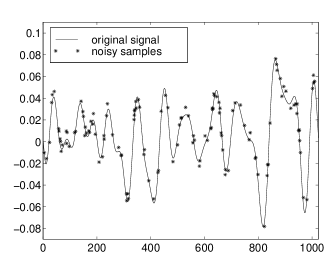
(a) Original signal and perturbed samples

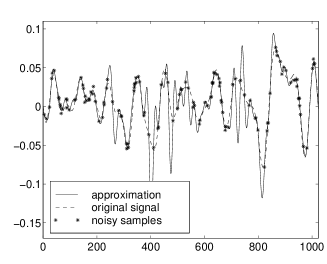
(b) Least squares approximation using a too large upper bound for the degree of the polynomial (overfit)

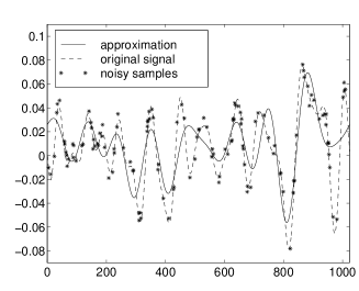
(c) Least squares approximation using a too small upper bound for the degree of the polynomial (underfit)

(d) Regularized approximation by proposed Levinson-Galerkin algorithm

Fig. 1: Controlling the smoothness of the solution is essential for trigonometric approximation from perturbed data in order to avoid overfitting and underfitting of the data. The proposed Levinson-Galerkin algorithm automatically adapts to the least squares solution of optimal degree.

The paper is organized as follows. In Sections 2 and 4 we present the main results, including the Levinson-Galerkin algorithm and a theoretical analysis that clarifies under which conditions this algorithm provides optimal results. In Section 3 we show how properly chosen weights can be used as simple but efficient tool to precondition the least squares problem. Some aspects of extending the algorithm to multivariate trigonometric polynomials are discussed in 5. In Section 6 we present some applications in echocardiography.

Before we proceed we introduce some notation and conventions. The inner product is denoted by $\langle\cdot,\cdot\rangle$, and the conjugate transpose of a matrix $A$ by $A^{\ast}$. The space of trigonometric polynomial of degree equal to or less than $M$ is defined as

$${{\boldsymbol{P}}_{\!M}}=\left\{p:p(x)=\sum_{k=-M}^{M}c_{k}e^{2\pi ikx}\right\}\,.$$ (2)

The norm of $p(x)=\sum_{k=-M}^{M}c_{k}e^{2\pi ikx}\in{{\boldsymbol{P}}_{\!M}}$ is given by

$$\|p\|=\left(\int\limits_{0}^{1}|p(x)|^{2}\,dx\right)^{\frac{1}{2}}=\left(\sum_{k=-M}^{M}|c_{k}|^{2}\right)^{\frac{1}{2}}=\|c\|\,,$$ (3)

where $c=\{c_{k}\}_{k=-M}^{M}$. In some applications it is advantageous to deal with complex-valued polynomials (see also Section 6), hence we do not restrict ourselves to the case of real-valued trigonometric approximation.

For $a=[a_{-M},a_{-M+1},\dots,a_{M-1},a_{M}]\in{{\mathbb{C}}^{2M+1}}$ we define the orthogonal projections ${P_{N}}$ by

$${P_{N}}a=[0,\dots,0,a_{-N},a_{-N+1},\dots,a_{N-1},a_{N},0,\dots,0]$$ (4)

for $N=1,2,\dots,M$ and identify the image of ${P_{N}}$ with the $2N+1$-dimensional space ${\mathbb{C}}^{2N+1}$.

Let $p^{M}$ and $p^{N}$ be trigonometric polynomials of degree $M$ and $N$ respectively, with coefficients vectors $c^{M}\in{\mathbb{C}}^{2M+1},c^{N}\in{\mathbb{C}}^{2N+1}$. If $N<M$, then we can always interpret $p^{N}$ as polynomial of degree $M$ by adding to appropriate number of zero-coefficients and by doing so we are embedding the vector $c^{N}$ into a zero-padded vector of length $2M+1$. We will henceforth tacitly assume that such an embedding has been made, when we compute expressions such as $\|c^{M}-c^{N}\|$.

2 Multi-level least squares approximation

A standard method in numerical analysis to find the optimal balance between fitting the given data and preserving smoothness of the solution is to introduce a regularization parameter. The best value of this regularization parameter is then determined for instance by generalized cross validation [15] or via the L-curve [20]. Here we understand regularization not as a way to stabilize ill-conditioned problems, but in a broader context as a means of finding the best compromise between fitting a given set of data and preserving smoothness of the solution. As we will see, in our case it is not necessary to introduce an additional parameter, since we can regularize the smoothness of the solution by varying the parameter $M$ of the space ${{\boldsymbol{P}}_{\!M}}$ in which we are searching for the solution of (1).

For the derivation of the algorithm we consider first the following situation. Assume $p_{*}(x)=\sum_{k=-N_{*}}^{N_{*}}(c_{*})_{k}e^{2\pi ikx}\in{{\boldsymbol{P}}}_{\!N_{*}}$ and let $s^{\varepsilon}=\{s^{\varepsilon}_{j}\}_{j=1}^{r},2M+1\leq r$ with $s^{\varepsilon}_{j}=s_{j}+\nu_{j}=p_{*}(x_{j})+\nu_{j}$ be given noisy samples satisfying

$$\|s^{\varepsilon}-s\|^{2}\leq\varepsilon\|s^{\varepsilon}\|^{2}.$$ (5)

For convenience we assume that $r$, the number of samples, is odd.

The aim is to approximate $p_{*}$ from the data $\{s^{\varepsilon}_{j}\}_{j=1}^{r}$. Let us first assume that we already know that we are searching for our least squares solution in the space ${{\boldsymbol{P}}}_{\!N_{*}}$. In this case the coefficient vector of the polynomial that solves (1) is the least squares solution of

$$WV_{N_{*}}c=Ws^{\varepsilon}\,,$$ (6)

where $V_{N_{*}}$ is a $r\times(2N_{*}+1)$ Vandermonde matrix with entries

$$(V_{M})_{j,k}=e^{2\pi ikx_{j}},\qquad j=1,\dots,r,\,k=-N_{*},\dots,N_{*}$$ (7)

and $W=\mathop{\operator@font diag}\nolimits(\{\sqrt{w_{j}}\})$.

We will discuss the role and specific choice of the weights in more detail in Section 3. To reduce the notational burden we absorb the weight matrix $W$ in the Vandermonde matrix and in the sampling values. Thus for given degree, $M$ say, we consider the linear system of equations

$$V_{M}c=s^{\varepsilon}\,$$ (8)

where $V_{M}$ is now the $r\times(2M+1)$ “weighted Vandermonde” matrix. We will denote the least squares solution of (8) by $c^{(M)}=\{c^{(M)}_{k}\}_{k=-M}^{M}$ and the corresponding polynomial is $p^{(M)}(x)=\sum_{k=-M}^{M}c^{(M)}_{k}e^{2\pi ikx}$.

Since in general we do not know the optimal degree or level $M$ of the space ${{\boldsymbol{P}}_{\!M}}$ in which we should solve the least squares problem, the situation becomes considerably more complicated. If we want to solve (1) under the information (5) without knowing the degree of the polynomial, one may argue that we have to accept any trigonometric polynomial $p(x)=\sum_{k=-N}^{N}c_{k}e^{2\pi ikx}$ with $\|V_{N}c-s^{\varepsilon}\|\leq\varepsilon\|s^{\varepsilon}\|$ as an approximate solution to $p_{*}$, since it is compatible with the only knowledge we have on the data.

In general there may be infinitely many such polynomials, which raises the questions of how to find a polynomial $p$ that yields a small approximation error $\|p_{*}-p\|$ and at the same time can be computed efficiently.

2.1 A multi-level algorithm and an efficient stopping criterion

The heuristic considerations above suggest the following approach.

Algorithm 1.

Set $N=0$ and solve $V_{0}c^{(0)}=s^{\varepsilon}$. If $c^{(0)}$ satisfies the condition $\|V_{0}c^{(0)}-s^{\varepsilon}\|\leq\varepsilon\|s^{\varepsilon}\|$, take $c^{(0)}$ as solution. Otherwise set $N=N+1$ and solve

$$V_{N}c^{(N)}=s^{\varepsilon}\,,$$ (9)

until $c^{(N)}$ satisfies for the first time the stopping criterion

$$\|V_{N}c^{(N)}-s^{\varepsilon}\|\leq\varepsilon\|s^{\varepsilon}\|.$$ (10)

at some level $N=N_{0}$. Set $c^{(N_{0})}=c^{(N)}$. The approximation to $p_{*}$ is then $p^{(N_{0})}(x)=\sum_{k=-M}^{M}c^{(N_{0})}_{k}e^{2\pi ikx}$.

The stopping criterion (10) is well-defined, since it is definitely satisfied for $N=(r-1)/2$, in which case the left side in (10) equals 0. Thus Algorithm 1 selects among all least squares solutions $p^{(N)},N=0,\dots,(r-1)/2$ that polynomial with minimal degree.

Algorithm 1 and stopping criterion (10) can be justified by the following theoretical considerations.

One readily verifies that the matrices $V_{N},N=0,\dots,(r-1)/2$ satisfy the relations:

• there exists a left-inverse $V_{N}^{+}$ such that

  $$V_{N}^{+}V_{N}=I_{N},\quad\text{with}\,\,V_{N}^{+}=(V_{N}^{\ast}V_{N})^{-1}V_{N}^{\ast},$$ (11)

  where $I_{N}$ is the identity matrix on ${{\mathbb{C}}^{2N+1}}$.

• Let $a\in{{\mathbb{C}}^{2M+1}}$ be the coefficient vector of some $p\in{{\boldsymbol{P}}_{\!M}}$. Then

  $$V_{N}a=V_{M}a\qquad\text{for all}\,\,N>M,\,a\in{{\mathbb{C}}^{2M+1}}.$$ (12)

In (ii) we have made use of the fact that the coefficient vector $a$ can be interpreted as coefficient vector of a polynomial of degree $N$ by extending it to a vector of length $2N+1$ via zero-padding. The matrix-vector multiplication $V_{M}a$ and equation (12) should be understood in this sense.

Lemma 1.

If $N\geq N_{*}$ then $c^{(N)}$ satisfies $\|V_{N}c^{(N)}-s^{\varepsilon}\|\leq\varepsilon\|s^{\varepsilon}\|$, hence stopping criterion (10) always becomes active at some level $N_{0}\leq N_{*}$.

Proof.

Note that $V_{N}V_{N}^{+}$ is the orthogonal projection into $\operatorname{range}(V_{N})$ and $s\in\operatorname{range}(V_{N_{*}})\subseteq\operatorname{range}(V_{N})$ for $N_{*}\leq N$, hence $V_{N}V_{N}^{+}s=s$. Therefore

$$\|V_{N}c^{(N)}-s^{\varepsilon}\|^{2}= \|V_{N}V_{N}^{+}(s+\nu)-(s+\nu)\|^{2}=\|\nu-V_{N}V_{N}^{+}\nu\|^{2}$$ (13)

$$= \|\nu\|^{2}-\|V_{N}V_{N}^{+}\nu\|^{2}\leq\varepsilon^{2}\|s^{\varepsilon}\|^{2},$$ (14)

where we have used condition (5) in the last step. It follows from (14) that Algorithm 1 terminates at some level $N_{0}\leq N_{*}$. ∎

The following lemma shows that from the viewpoint of numerical stability it is advisable to keep the level $N$ of the space ${{\boldsymbol{P}}_{\!N}}$ in which we search for our solution as small as possible.

Lemma 2.

$\mbox{cond\/}(V_{N}^{\ast}V_{N})\geq\mbox{cond\/}(V_{M}^{\ast}V_{M})$ for $N\geq M$.

Proof.

Since

$${P_{M}}(V_{N}^{\ast}V_{N}){P_{M}}=V_{M}^{\ast}V_{M}\quad\text{for}\,\,M\leq N,$$

Cauchy’s Interlace Theorem [16] implies that $\mbox{cond\/}(V_{N}^{\ast}V_{N})\geq\mbox{cond\/}(V_{M}^{\ast}V_{M})$ for $N\geq M$. ∎

In the sequel we demonstrate that the fact that Algorithm 1 terminates at some level $\leq N_{*}$ is a desired property in many cases. We show that stopping criterion (10) is even optimum in a number of cases.

Let us first consider two special cases: (i) noisefree samples and (ii) uniformly spaced samples.

2.1.1 Noisefree samples

Any reasonable stopping criterion has to satisfy the following lemma.

Lemma 3.

For noisefree data the stopping criterion (10) yields the exact solution.

Proof.

One readily verifies that Algorithm 1 terminates at level $N_{*}$. Hence for $N=N_{*}$:

$$\|p^{(N)}-p_{*}\|=\|c^{(N)}-c_{*}\|=\|V_{N}^{+}s^{\varepsilon}-c_{*}\|=\|V_{N}^{+}V_{N}c_{*}-c_{*}\|=0,$$ (15)

since $V_{N}^{+}V_{N}c_{*}=c_{*}$ for $N\geq N_{*}$. ∎

Lemmas 3 and 2 together show that stopping criterion (10) yields the optimum solution for noisefree data while providing maximum numerical stability.

2.1.2 Uniformly spaced samples

If the sampling points $x_{j},j=1,\dots,r$ are uniformly spaced and we choose $w_{j}=1/r$ as weights then a simple calculation shows that $V_{N}$ is unitary on ${{\mathbb{C}}^{2N+1}}$, i.e., $V_{N}^{\ast}V_{N}=I_{N}$ for $N=0,1,\dots,(r-1)/2$.

In this case

$$\|c_{*}-c^{(N)}\|=\|c_{*}-V_{N}^{\ast}s^{\varepsilon}\|=\|c_{*}-V_{N}^{\ast}V_{N_{*}}c_{*}-V_{N}^{\ast}\nu\|.$$ (16)

$N\geq N_{*}$ implies $V_{N}^{\ast}V_{N_{*}}=I_{N}$ and hence

$$\|c_{*}-c^{(N)}\|=\|V_{N}^{\ast}\nu\|.$$ (17)

Note that

$$\|V_{N}^{\ast}\nu\|=\langle V_{N}^{\ast}\nu,V_{N}^{\ast}\nu\rangle=\langle V_{N}V_{N}^{\ast}\nu,\nu\rangle=\|V_{N}V_{N}^{\ast}\nu\|,$$ (18)

since $V_{N}V_{N}^{\ast}$ is an orthogonal projection. Equation (18) yields

$$\|V_{M}^{\ast}\nu\|\leq\|V_{N}^{\ast}\nu\|\qquad\text{for}\,\,\,M\leq N,.$$ (19)

Consequently

$$\|c_{*}-c^{(M)}\|\leq\|c_{*}-c^{(N)}\|\qquad\text{if}\,\,\,N_{*}\leq M\leq N.$$ (20)

Thus for uniformly spaced samples any stopping criterion should terminate Algorithm 1 at the latest at $N=N_{*}$. Under a mild condition on the coefficients $c_{*}$ we can show that the proposed stopping criterion provides the optimal solution among all least squares solutions.

Proposition 4.

Assume that the samples are regularly spaced. Then the solution $p^{(N_{0})}$ computed via Algorithm 1 satisfies

$$\|p_{*}-p^{(N_{0})}\|\leq\|p_{*}-p^{(N)}\|\qquad\text{for all}\,\,\,N\geq N_{*}.$$ (21)

If furthermore $p_{*}$ satisfies

$$\|(I_{N_{*}}-{P_{N}})c_{*}\|\geq\|(I_{N_{*}}-{P_{N}})V_{N_{*}}^{\ast}\nu\|$$ (22)

then

$$\|p_{*}-p^{(N_{0})}\|\leq\|p_{*}-p^{(N)}\|\qquad\text{for all}\,\,N.$$ (23)

Condition (22) is satisfied e.g., if all coefficients of $p_{*}$ are larger than the relative noise level, i.e., $|c_{k}|\geq\varepsilon\|s^{\varepsilon}\|$.

Proof.

Lemma 1 yields that $N_{0}\leq N_{*}$, thus (20) implies (21).

To prove assertion (23) we only have to show that

$$\|c_{*}-c^{(N_{0})}\|\leq\|c_{*}-c^{(N)}\|\qquad\text{for all}\,\,N<N_{*}$$

For $N<N_{*}$ note that $(c_{*}-V_{N}^{\ast}V_{N_{*}}c_{*})$ is orthogonal to $V_{N}^{\ast}\nu$, since

$$\langle c_{*},V_{N}^{\ast}\nu\rangle= \langle V_{N_{*}}^{\ast}V_{N_{*}}c_{*},V_{N}^{\ast}\nu\rangle$$ (24)

$$= \langle V_{N_{*}}c_{*},V_{N_{*}}^{\ast}V_{N}^{\ast}\nu\rangle=\langle V_{N_{*}}c_{*},V_{N}V_{N}^{\ast}\nu\rangle,$$ (25)

hence

$$\langle c_{*}-V_{N}^{\ast}V_{N_{*}}c_{*},V_{N}^{\ast}\nu\rangle=0.$$

Therefore

$$\|c_{*}-c^{(N)}\|^{2}=\|c_{*}-V_{N}^{+}V_{N_{*}}c_{*}+V_{N}^{\ast}\nu\|^{2}=\|c_{*}-V_{N}^{+}V_{N_{*}}c_{*}\|^{2}+\|V_{N}^{\ast}\nu\|^{2}\,.$$

In order to prove $\|c_{*}-c^{(N_{0})}\|\leq\|c_{*}-c^{(N)}\|$ for all $N<N_{*}$ we need to verify $\|c_{*}-V_{N}^{+}V_{N_{*}}c_{*}\|^{2}+\|V_{N}^{\ast}\nu\|^{2}\geq\|V_{N_{*}}^{\ast}\nu\|^{2}$. Since

$$\|c_{*}-V_{N}^{+}V_{N_{*}}c_{*}\|^{2}=\sum_{|k|=N+1}^{N_{*}}|(c_{*})_{k}|^{2}=\|(I_{N}-{P_{N}})c_{*}\|^{2}$$

and

$$\|(V_{N_{*}})^{\ast}\nu\|^{2}-\|V_{N}^{\ast}\nu\|^{2}=\sum_{|k|=N+1}^{N_{*}}|(V_{N_{*}}^{\ast}\nu)_{k}|^{2}=\|(I_{N}-{P_{N}})V_{N_{*}}^{\ast}\nu\|^{2},$$

the result follows now from the assumption (22). ∎

Remark:  Proposition 4 shows that the least squares polynomial that gives the best approximation to $p_{*}$ is not necessarily of degree $N_{*}$.

2.1.3 Noisy nonuniform samples

For noisy nonuniformly spaced data we observe that

$$\|p_{*}-p^{(N)}\|=\|c_{*}-c^{(N)}\|\leq\|c_{*}-V_{N}^{+}V_{N_{*}}c_{*}\|+\|V_{N}^{+}\nu\|,$$

and for $N\geq N_{*}$

$$\|p_{*}-p^{(N)}\|\leq\|V_{N}^{+}\nu\|,$$ (26)

since $\|c_{*}-V_{N}^{+}V_{N_{*}}c_{*}\|=0$ in this case.

If $V_{N}$ is not unitary then $\|V_{N}^{+}\nu\|$ is not necessarily monotonically increasing with increasing level $N$. One can argue heuristically that since $\|V_{N}^{+}\|$ is increasing with increasing level $N$ due to Lemma 2, we may fairly assume that $\|V_{N}^{+}\nu\|$ will also increase (although not strictly monotonically). Also from the viewpoint of numerical stability it is reasonable to keep the level $N$ small, since by Lemma 2 we know that $\mbox{cond\/}(V_{N}^{\ast}V_{N})\geq\mbox{cond\/}(V_{M}^{\ast}V_{M})$ for $N\geq M$. This together with (26) suggests to choose a stopping criterion which terminates at or before level $N_{*}$, which is guaranteed for stopping criterion (10) by Lemma 1.

We can conclude that the stopping criterion will provide excellent results if the noise level $\varepsilon$ is small or if the condition number of $V_{N}^{\ast}V_{N}$ is small (which implies that $V_{N}$ is approximately unitary). In order to verify the latter it is useful to have estimates for the condition number of $V_{N}^{\ast}V_{N}$. We will address this issue in Proposition 40.

2.2 A Toeplitz system and trigonometric approximation

Instead of directly solving $V_{M}c^{(M)}=s^{\varepsilon}$ it is more efficient in our case to consider the normal equations

$$V_{M}^{\ast}V_{M}^{\ast}c^{(M)}=V_{M}^{\ast}s^{\varepsilon}.$$ (27)

The reason is that from a numerical point of view the structural properties of the matrix $V_{M}^{\ast}V_{M}$ are much more attractive than those of $V_{M}$, which in turn leads to faster numerical algorithms, see also Section 4.

Set $T_{M}=V_{M}^{\ast}V_{M}$ then a simple calculation shows that the entries of the hermitian matrix $T_{M}$ are

$$(T_{M})_{k,l}=\sum_{j=1}^{r}w_{j}e^{2\pi i(k-l)x_{j}},\qquad k,l=-M,\dots,M.$$ (28)

$T_{M}$ is a Toeplitz matrix, since the entries $(T_{M})_{k,l}$ depend only on the difference $k-l$. Obviously $T_{M}$ is invertible if $2M+1\leq r$.

Following result is just a reformulation of (27) together with relation (12), but since it plays a key role in Section 4 it is helpful to state it in detail (cf. also [18]).

Theorem 5.

Given the sampling points $0\leq x_{1}<\dots,x_{r}<1$, samples $\{s^{\varepsilon}_{j}\}_{j=1}^{N}$, positive weights $\{w_{j}\}_{j=1}^{r}$ and the degree $M$ with $2M+1\leq r$. The polynomial $p^{(M)}\in{{\boldsymbol{P}}_{\!M}}$ that solves (1) is given by

$$p^{(M)}(x)=\sum_{k=-M}^{M}c^{(M)}_{m}e^{2\pi ikx}\in{{\boldsymbol{P}}_{\!M}}\,.$$ (29)

where its coefficients $c^{(M)}_{k}$ satisfy

$$T_{M}c^{(M)}=b^{(M)}\,\,\in{\mathbb{C}}^{(2M+1)^{2}},$$ (30)

with

$$b^{(M)}_{k}=\sum_{j=1}^{r}s^{\varepsilon}_{j}w_{j}e^{2\pi ikx_{j}}\qquad\mbox{for $|k|\leq M$},$$ (31)

and $T_{M}$ as defined in (28).

3 Weights as simple preconditioner

Vandermonde matrices are known to be ill-conditioned, if the nodes $x_{j}$ are clustered [13]. To improve the stability of the systems (8) and (30) we can use the weights as simple diagonal preconditioner. This leads to the problem of how to choose the weights $w_{j}$.

We propose to use the size of the area of the Voronoi region [23] associated with the sampling point $x_{j}$ as weight $w_{j}$. In 1-D this reduces to

$$w_{j}=\frac{x_{j+1}-x_{j-1}}{2}\,.$$ (32)

This choice is motivated by the following observations.

In this section we let $V_{N}$ denote the Vandermonde matrix defined in (7) without weights. Let $p\in{{\boldsymbol{P}}_{\!M}}$ with coefficient vector $c$. Since

$$\langle T_{M}c,c\rangle=\langle WV_{M}c,WV_{M}c\rangle=\|WV_{M}c\|^{2}=\sum_{j=1}^{r}|p(x_{j})|^{2}w_{j},$$ (33)

the inequality

$$C_{1}\|c\|^{2}\leq\sum_{j=1}^{r}|p(x_{j})|^{2}w_{j}\leq C_{2}\|c\|^{2}$$ (34)

holds for all $c\in{\mathbb{C}}^{2M+1}$ with constants $C_{1}=\lambda_{min}$ and $C_{2}=\lambda_{max}$, where $\lambda_{min}$ and $\lambda_{max}$ denote the minimal and maximal eigenvalue, respectively, of $T_{M}$.

(i) The lower bound of $T_{M}$ is mainly determined by the large gaps in the sampling set. Suppose there is a large gap in the sampling set and denote the interval corresponding to this gap by $\Gamma$ (hence $x_{j}\notin\Gamma$). Choose a trigonometric polynomial $p\in{{\boldsymbol{P}}_{\!M}}$ which, like the prolate spheroidal functions, concentrates most of its energy in the interval $\Gamma$. Then the sampling values of $p$ will not pick up any information about the main concentration of the polynomial energy. Consequently if we use no weights (or set $w_{j}=1$) we get

$$\sum_{j\notin\Gamma}|p(x_{j})|^{2}\ll\|p\|^{2}=\|c\|^{2}.$$

For such a sampling set the lower frame bound $C_{1}$ in the inequality (34) must be small. Generically, large gaps and the ensuing lack of information always results in bad condition numbers. This problem cannot be fixed by preconditioning.

(ii) On the other hand, we can choose a trigonometric polynomial that is mainly concentrated in the region where the sampling points are located. In this case the same local information is counted and added several times. Thus

$$\sum_{j\notin\Gamma}|p(x_{j})|^{2}\gg\|p\|^{2}=\|c\|^{2}$$

and the upper constant $C_{2}$ in (34) will be large. Yet, as mentioned in (i) a cluster will not contribute much to the lower bound and to the uniqueness of the problem. In this case the condition number is large, because too much local information is given in certain areas of the polynomial.

Problem (ii) can be addressed by introducing properly chosen weights. The idea is to compensate for the local variation of the sampling density by using weights in inequality (34). Suppose that $0\leq x_{1}\leq x_{2}\leq\dots\leq x_{r}<1$ is a sampling set in $[0,1]$. Then a natural choice for the weights is $w_{j}=(x_{j+1}-x_{j-1})/2$. Thus if many samples are clustered near a point $x_{j}$, then the weight $w_{j}$ is small. If $x_{j}$ is the only sampling point in a large neighborhood, then the corresponding weight is large. This choice has not only been confirmed by extensive numerical experiments [11], but also by the following optimization approach.

A standard approach for the construction of preconditioners for a matrix $A$ is the following. One attempts to find the matrix $P$ in a given class ${\cal M}$ of matrices (e.g., the class of all circulant matrices or the class of all diagonal matrices) which solves

$$\underset{P\in{\cal M}}{\min}\|I-PA\|_{F}\,,$$ (35)

where $\|.\|_{F}$ denotes the Frobenius norm.

In our setting this translates to the following optimization problem

$$\underset{W\in{\cal D}}{\min}\|I-(WV)^{\ast}WV\|_{F}\,,$$ (36)

where ${\cal D}$ is the class of all $r\times r$ diagonal matrices and $I$ is the $(2M+1)\times(2M+1)$ identity matrix.

Note that we require that $w_{j}>0$ whereas (36) could in principle yield weights that violate this condition. However since we will make use of  (36) in our actual algorithm, we are somewhat sloppy here.

An alternative approach is to consider the solution of

$$\begin{array}[]{c}\min\{\mbox{cond\/}[(WV)^{\ast}WV]\}\\ \mbox{subject to $W\in{\cal D}$}.\end{array}$$ (39)

This optimization problem can be transformed to a general eigenvalue problem, see [4], which can be solved by convex optimization algorithms.

In the simple case of regular sampling it is easy to check that the solution of both optimization problems is given by $W=\mathop{\operator@font diag}\nolimits(\{\sqrt{w_{j}}\})$ with $w_{j}=(x_{j+1}-x_{j-1})/2=1/r$. However in the more interesting case of nonuniform sampling neither problem (36) nor (39) does in general have an analytic solution. Thus using these approaches for the actual construction of a preconditioner would be ridiculous, since the computational costs to solve these optimization problems are considerably larger than solving the trigonometric approximation problem. Nevertheless, solving (36) and (39) numerically for a variety of different examples is useful to get insight in the type of weights obtained by these approaches.

The numerical results confirm the choice of the Voronoi-type weights defined in (32). Sampling points in densely sampled areas are assigned a small weight, whereas sampling points in sparse sampled regions are assigned a large weight. Two typical comparisons of the weights obtained via optimization and the Voronoi weights are illustrated in Figure 2. In the first case we consider a sampling set with high density at the endpoints and strongly decreasing density towards the center. The weights obtained by solving (36) and (39) are almost identical and are very close to the Voronoi weights, as can be seen in Figure 2(a). The difference at the endpoints is probably due to boundary effects.

In the second example we consider a random sampling set with several areas with high sampling density and relatively few samples between these clusters. Again all three approaches give weights that show a similar behavior, see Figure 2(b). The condition number of the non-weighted Toeplitz matrix in this example is 33, compared to the significantly smaller condition number 3.3 when using Voronoi-type weights. Using the weights obtained via (36) gives $\mbox{cond\/}(T_{M})=3.1$, and for the weights resulting from (39) we get $\mbox{cond\/}(T_{M})=2.9$, which is only a slight improvement compared to the Voronoi-type weights.

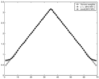
Fig. 2: Comparison of weights obtained by different approaches.

Obtaining good estimates for the condition number of a Toeplitz matrix is a difficult problem. It is gratifying that by using the weights defined in (32) it is possible to get an upper bound for the condition number.

Proposition 6 (Gröchenig, [18]).

Assume that the sampling set $\{x_{j}\}_{j=1}^{r}$ satisfies

$$\max(x_{j+1}-x_{j}):=\gamma<\frac{1}{2M}$$

and set $w_{j}=(x_{j+1}-x_{j-1})/2$. Then the condition number of the Toeplitz matrix $T_{M}$ defined in (28) is bounded by

$$\kappa(T_{M})\leq\left(\frac{1+\gamma}{1-\gamma}\right)^{2}\,.$$ (40)

4 A Levinson-Galerkin algorithm for trigonometric approximation

The method described in Algorithm 1 can be seen as a Galerkin-type approach, since we try to determine an approximation by searching for a solution in a finite-dimensional space spanned by orthogonal polynomials, and by increasing the dimension of the space we increase the resolution of our approximation by adding more and more details.

When we use Levinson’s algorithm [16] to solve (30) for $M=0,1,\dots,N_{0}$ the total computational effort would be of ${\cal O}(N_{0}^{3})$, since the solution of each system $T_{M}c^{(M)}=b^{(M)}$ requires ${\cal O}(M^{2})$ operations. Using one of the fast Toeplitz algorithms [2, 5] reduces this effort to ${\cal O}(kM\log M)$ for each level $M$, where $k$ is the number of iterations, thus leading to a total of ${\cal O}(kN_{0}^{2}\log N_{0})$ operations. In this section we show that the systems $T_{M}c^{(M)}=b^{(M)},M=0,1,\dots,N_{0}$ can be solved in ${\cal O}(N_{0}^{2})$ operations and the total effort (including the calculation of the entries of $T_{M}$ and the evaluation of the stopping criterion (10)) for computing $p^{(N_{0})}$ is ${\cal O}(rN_{0}+N_{0}^{2})$ operations.

Following observation is crucial for the derivation of the proposed Levinson-Galerkin algorithm.

Lemma 7.

For fixed degree $M$ and $M+1$ let $T_{M},b^{(M)}$ and $T_{M+1},b^{(M+1)}$ be the Toeplitz matrices and right hand sides as defined in (28) and (31), respectively. Then $T_{M}$ and $b^{(M)}$ are embedded in $T_{M+1}$ and $b^{(M+1)}$ in the following way:

$$T_{M+1}=\begin{bmatrix}t_{0}&\dots&{\overline{t}_{2(M+1)}}\\ \vdots&\framebox{$T_{M}$}&\vdots\\ t_{2(M+1)}&\dots&t_{0}\end{bmatrix},\,\,b^{(M+1)}=\begin{bmatrix}b_{-(M+1)}\\ \framebox{\!\!\!\!\!\!\!\!\!\! $b^{(M)}$\!\!\!\!\!\!\!\!\!}\\ b_{M+1}\end{bmatrix}.$$ (41)

Proof.

(41) follows immediately from the definition of $T_{M}$ and $b^{(M)}$ and (12). ∎

Unfortunately the solutions $c^{(M)}$ and $c^{(M+1)}$ of the systems $T_{M}c^{(M)}=b^{(M)}$ and $T_{M+1}c^{(M+1)}=b^{(M+1)}$ are not related is such a simple manner. But we can exploit the nested structure of the family $\{T_{M}\}_{M=1}^{N_{0}}$ by solving the systems $T_{M}c^{(M)}=b^{(M)}$ recursively via a modified Levinson algorithm. The standard Levinson algorithm cannot be applied directly, since it only addresses Toeplitz systems, where the principal leading sub-matrix and the principal leading sub-vector of the right hand side stay unchanged during the recursion, which is not the case here. For $T_{M+1}$ it does not matter, if we enlarge $T_{M}$ by appending new entries below or above, whereas the right hand side $b^{(M)}$ cannot be rearranged in such a way, the principal leading subvector of the right hand side will be changed if we switch from $b^{(M)}$ at level $M$ to $b^{(M+1)}$ at level $M+1$.

To adapt Levinson’s algorithm to our situation, we have to split up the change from the system $T_{M}c^{(M)}=b^{(M)}$ at level $M$ to the system $T_{M+1}c^{(M+1)}=b^{(M+1)}$ at level $M+1$ into two separate steps. Instead of indexing the matrix $T_{M}$ and the vectors $b^{(M)},c^{(M)}$ by the degree $M$, it is therefore advantageous to index them according to their dimension. For clarity of presentation we reserve the subscript $(M)$ for the degree of the polynomial and its coefficient vector respectively, and use the subscript $(\ell)$ when we refer to the dimension of the corresponding coefficient vector in ${\mathbb{C}}^{\ell}$. Thus for even $\ell$, $b^{(\ell)}=[b_{-\frac{\ell}{2}+1},\dots,b_{\frac{\ell}{2}}]^{T}\in{\mathbb{C}}^{\ell}$, and for odd $\ell$ we set $b^{(\ell)}=[b_{-\frac{\ell-1}{2}},\dots,b_{\frac{\ell-1}{2}}]^{T}$ (whence $b^{(1)}=b_{0}$), analogously for $c^{(\ell)}$. Further it is useful in the sequel to denote $t^{(\ell)}=[t_{1},\dots,t_{\ell}]^{T}$. Then the Toeplitz matrix $T_{\ell}$ of size $\ell\times\ell$ is generated by the vector $[t_{0},(t^{(\ell-1)})^{T}]^{T}$ with $t_{k}=\sum_{j=1}^{r}w_{j}e^{2\pi ikx_{j}}$ according to (28).

Assume we have already solved the system $T_{M}c^{(M)}=b^{(M)}$ at level $M$ (with $\ell=2M+1$) and now we want to switch to the next level $M+1$. As we have agreed, we do this in two steps. In the first step ($\ell\rightarrow\ell+1$) the Toeplitz system can be written as

$$\begin{bmatrix}T_{\ell}&E_{\ell}\overline{t^{(\ell)}}\\ (t^{(\ell)})^{T}E_{\ell}&t_{0}\end{bmatrix}\begin{bmatrix}v^{(\ell)}\\ v_{\frac{\ell+1}{2}}\end{bmatrix}=\begin{bmatrix}b^{(\ell)}\\ b_{\frac{\ell+1}{2}}\end{bmatrix}\,,$$ (42)

where $E_{\ell}$ is the rotated identity matrix on ${\mathbb{C}}^{\ell}$, i.e.,

$$E_{\ell}=\begin{bmatrix}0&&1\\ &\mathinner{\mkern 1.0mu\raise 1.0pt\vbox{\kern 7.0pt\hbox{.}}\mkern 2.0mu\raise 4.0pt\hbox{.}\mkern 2.0mu\raise 7.0pt\hbox{.}\mkern 1.0mu}&\\ 1&&0\end{bmatrix}\,.$$

System (42) can be solved recursively by the standard Levinson algorithm [21, 16]. To be more detailed, assume that we have already solved the system $T_{\ell}c^{(\ell)}=b^{(\ell)}$ for $\ell=2M+1$ and assume further that the solution of the $\ell$-th order Yule-Walker system $T_{\ell}y^{(\ell)}=-t^{(\ell)}$ is available. Then the solution of (42) can be computed recursively by

$$v_{\frac{\ell+1}{2}} =(b_{\frac{\ell+1}{2}}-[t^{(\ell)}]^{T}E_{\ell}c^{(\ell)})/\beta_{\ell}$$

$$v^{(\ell)} =c^{(\ell)}+v_{\frac{\ell+1}{2}}E_{\ell}{\overline{y}^{(\ell)}}$$

where

$$\beta_{\ell} =t_{0}+[t^{(\ell)}]^{T}{\overline{y}^{(\ell)}}=(1-\alpha_{\ell-1}{\overline{\alpha}_{\ell-1}})\beta_{\ell-1}$$

$$\alpha_{\ell} =-(t_{\ell+1}+[t^{(\ell)}]^{T}E_{\ell}y^{(\ell)})/\beta_{\ell}$$

$$z^{(\ell)} =y^{(\ell)}+\alpha_{\ell}E_{\ell}{\overline{y}^{(\ell)}}$$

$$y^{(\ell+1)} =\begin{bmatrix}z^{(\ell)}\\ \alpha_{\ell}\end{bmatrix}\,.$$

Now we can proceed to the second step ($\ell+1\rightarrow\ell+2=2(M+1)+1$), where the Toeplitz system can be expressed as

$$\begin{bmatrix}t_{0}&(t^{(\ell+1)})^{\ast}\\ t^{(\ell+1)}&T_{\ell+1}\end{bmatrix}\begin{bmatrix}v_{-\frac{\ell+1}{2}}\\ v^{(\ell+1)}\end{bmatrix}=\begin{bmatrix}b_{-\frac{\ell+1}{2}}\\ b^{(\ell+1)}\end{bmatrix}$$ (43)

with $c^{(\ell+2)}=[v_{-\frac{\ell+1}{2}},(v^{(\ell+1)})^{T}]^{T}=c^{(M+1)}$. Observe that (43) cannot be transformed to a system of the form (42) by simple permutations, i.e. just by interchanging rows and columns. Since we have already solved the systems $T_{\ell+1}c^{(\ell+1)}=b^{(\ell+1)}$ and $T_{\ell+1}y^{(\ell+1)}=-t^{(\ell+1)}$ we can write

$$v^{(\ell+1)}=(T_{\ell+1})^{-1}(b^{(\ell+1)}-t^{(\ell+1)}v_{-\frac{\ell+1}{2}})=c^{(\ell+1)}+v_{-\frac{\ell+1}{2}}y^{(\ell+1)}$$

and

$$v_{-\frac{\ell+1}{2}}= (b_{-\frac{\ell+1}{2}}-[t^{(\ell+1)}]^{\ast}v^{(\ell+1)})/t_{0}$$

$$= (b_{-\frac{\ell+1}{2}}-[t^{(\ell+1)}]^{\ast}c^{(\ell+1)}-[t^{(\ell+1)}]^{\ast}v_{-\frac{\ell+1}{2}}y^{(\ell+1)})/t_{0}$$

$$= (b_{-\frac{\ell+1}{2}}-[t^{(\ell+1)}]^{\ast}c^{(\ell+1)})/\beta_{\ell+1}\,,$$

where we have used in the last step that $T_{\ell}=[T_{\ell}]^{\ast}$ which implies that $(t^{(\ell+1)})^{\ast}y^{(\ell+1)}$ is real and therefore $t_{0}+(t^{(\ell+1)})^{\ast}y^{(\ell+1)}=t_{0}+(t^{(\ell+1)})^{T}{\overline{y}^{(\ell+1)}}=\beta_{\ell+1}$.

Note that at each level $M$ we have to check if the stopping criterion (10) is satisfied. The evaluation of the expression

$$\sum_{j=1}^{r}|p^{(M)}(x_{j})-s^{\varepsilon}_{j}|^{2}w_{j}$$ (44)

can be considerably simplified and by avoiding the evaluation of $p^{(M)}$ at the nonuniformly spaced points $x_{j}$ we can reduce the computational effort from ${\cal O}(Mr)$ to ${\cal O}(M)$ operations.

To do this we define the subspace ${\cal R}=\big{\{}\{p(x_{j})\}_{j=1}^{r}:p\in{{\boldsymbol{P}}_{\!M}}\big{\}}\subseteq{\mathbb{C}}^{r}$ with the weighted inner product $\langle y,z\rangle_{{\cal R}}=\sum_{j=1}^{r}y_{j}\bar{z}_{j}w_{j}$ for $y,z\in{\mathbb{C}}^{r}$. The solution of the least squares problem (1) is the orthogonal projection of the vector $\{s^{\varepsilon}_{j}\}_{j=1}^{r}\in{\mathbb{C}}^{r}$ onto ${\cal R}$ and therefore must satisfy

$$\langle\{p^{(M)}(x_{j})\}-\{s^{\varepsilon}_{j}\},\{p^{(M)}(x_{j})\}\rangle_{\cal R}=\sum_{j=1}^{r}(p^{(M)}(x_{j})-s^{\varepsilon}_{j})\overline{p^{(M)}(x_{j})}w_{j}=0$$

which implies

$$\langle\{p^{(M)}(x_{j})\},\{s^{\varepsilon}_{j}\}\rangle_{\cal R}=\langle\{p^{(M)}(x_{j})\},\{p^{(M)}(x_{j})\}\rangle_{\cal R}\,.$$ (45)

Since

$$\sum_{j=1}^{r}|s^{\varepsilon}_{j}-p^{(M)}(x_{j})|^{2}w_{j}= \sum_{j=1}^{r}|s^{\varepsilon}_{j}|^{2}w_{j}-2\,\mbox{Re}\,\langle s^{\varepsilon},\{p^{(M)}(x_{j})\}\rangle_{\cal R}+\sum_{j=1}^{r}|p^{(M)}(x_{j})|^{2}w_{j}$$

$$= \sum_{j=1}^{r}|s^{\varepsilon}_{j}|^{2}w_{j}-\sum_{j=1}^{r}|p^{(M)}(x_{j})|^{2}w_{j}$$

by (45), and because

$$\sum_{j=1}^{r}|p^{(M)}(x_{j})|^{2}w_{j} =\sum_{j=1}^{r}w_{j}\bigg{(}\sum_{m=-M}^{M}c^{(M)}_{m}e^{2\pi imx_{j}}\bigg{)}\bigg{(}\sum_{n=-M}^{M}\overline{c^{(M)}_{n}}e^{2\pi inx_{j}}\bigg{)}$$

$$=\sum_{m=-M}^{M}\sum_{n=-M}^{M}c^{(M)}_{m}\overline{c^{(M)}_{n}}\bigg{(}\sum_{j=1}^{r}w_{j}e^{2\pi i(m-n)x_{j}}\bigg{)}$$

$$=\langle T_{M}c^{(M)},c^{(M)}\rangle=\langle b^{(M)},c^{(M)}\rangle\,,$$ (46)

it follows that

$$\sum_{j=1}^{r}|s^{\varepsilon}_{j}-p^{(M)}(x_{j})|^{2}w_{j}=\sum_{j=1}^{r}|s^{\varepsilon}_{j}|^{2}w_{j}-\langle b^{(M)},c^{(M)}\rangle\,.$$ (47)

Since $\sum_{j=1}^{r}|s^{\varepsilon}_{j}|^{2}w_{j}$ has to be computed only once at the beginning of the algorithm, the evaluation of (44) can be carried out in ${\cal O}(M)$ operations.

Summing up we have arrived at the following algorithm to compute $p^{(N_{0})}$.

Algorithm 2 (Levinson-Galerkin algorithm for trigonometric polynomials).

Let the sampling points $\{x_{j}\}_{j=1}^{r}$, sampling values $\{s^{\varepsilon}_{j}\}_{j=1}^{r}$, weights $w_{j}>0$ and the data error estimate $\varepsilon$ be given. Then the trigonometric polynomial $p^{(N_{0})}$ determined in Algorithm 1 can be computed in ${\cal O}(rN_{0}+N_{0}^{2})$ operations by the following algorithm.

Initialize: $t_{0}=\sum_{j=1}^{r}w_{j},t_{1}=\sum_{j=1}^{r}w_{j}e^{2\pi ix_{j}},b_{0}=\sum_{j=1}^{r}s^{\varepsilon}_{j}w_{j},\sigma=\sum_{j=1}^{r}|s^{\varepsilon}_{j}|^{2}w_{j}$, $y^{(1)}=-t_{1}/t_{0},c^{(1)}=b_{0}/t_{0},\beta_{0}=t_{0},\alpha_{0}=-t_{1}/t_{0},\varepsilon_{1}=(\sigma-b_{0}^{2}/t_{0})/\sigma,\ell=1$.

$$\mbox{\bf while}\ \,\varepsilon_{\ell}>\varepsilon$$

$$\qquad\beta_{\ell}=(1-\alpha_{\ell-1}{\overline{\alpha}_{\ell-1}})\beta_{\ell-1}$$

$$\qquad\mbox{\bf if}\ \ell\equiv 1\!\!\!\mod 2$$

$$\qquad\qquad b_{\frac{\ell+1}{2}}=\sum_{j=1}^{r}s^{\varepsilon}_{j}w_{j}e^{\pi i(\ell+1)x_{j}}$$

$$\qquad\qquad v_{\frac{\ell+1}{2}}=\frac{b_{\frac{\ell+1}{2}}-\langle E_{\ell}\overline{c^{(\ell)}},t^{(\ell)}\rangle}{\beta_{\ell}}$$

$$\qquad\qquad v^{(\ell)}=c^{(\ell)}+v_{\frac{\ell+1}{2}}E_{\ell}\overline{y^{(\ell)}}$$

$$\qquad\qquad c^{(\ell+1)}=\begin{bmatrix}v^{(\ell)}\\ v_{\frac{\ell+1}{2}}\end{bmatrix}$$

$$\qquad\qquad b^{(\ell+1)}=\begin{bmatrix}b^{(\ell)}\\ b_{\frac{\ell+1}{2}}\end{bmatrix}$$

$$\qquad{\bf elseif}\ \,\ell\equiv 0\!\!\!\mod 2$$

$$\qquad\qquad b_{-\frac{\ell}{2}}=\sum_{j=1}^{r}s^{\varepsilon}_{j}w_{j}e^{-\pi i\ell x_{j}}$$

$$\qquad\qquad v_{-\frac{\ell}{2}}=\frac{b_{-\frac{\ell}{2}}-\langle\overline{c^{(\ell)}},t^{(\ell)}\rangle}{\beta_{\ell}}$$

$$\qquad\qquad v^{(\ell)}=c^{(\ell)}+v_{-\frac{\ell}{2}}y^{(\ell)}$$

$$\qquad\qquad c^{(\ell+1)}=\begin{bmatrix}v_{-\frac{\ell}{2}}\\ v^{(\ell)}\end{bmatrix}$$

$$\qquad\qquad b^{(\ell+1)}=\begin{bmatrix}b_{-\frac{\ell}{2}}\\ b^{(\ell)}\end{bmatrix}$$

$$\qquad\qquad\varepsilon_{\ell+1}=|\sigma-\langle b^{(\ell+1)},c^{(\ell+1)}\rangle|/\sigma$$

end

$$\qquad t^{(\ell+1)}=\sum_{j=1}^{r}w_{j}e^{2\pi i(\ell+1)x_{j}}$$

$$\qquad\alpha_{\ell}=-\frac{t^{(\ell+1)}+\langle E_{\ell}\overline{y^{(\ell)}},t^{(\ell)}\rangle}{\beta_{\ell}}$$

$$\qquad z^{(\ell)}=y^{(\ell)}+\alpha_{\ell}E_{\ell}\overline{y^{(\ell)}}$$

$$\qquad y^{(\ell+1)}=\begin{bmatrix}z^{(\ell)}\\ \alpha_{\ell}\end{bmatrix}$$

$$\qquad t^{(\ell+1)}=\begin{bmatrix}t^{(\ell)}\\ t_{\ell+1}\end{bmatrix}$$

$$\qquad\ell=\ell+1$$

end

$$N_{0}=\ell/2$$

$$p^{(N_{0})}(x)=\sum_{k=-N_{0}}^{N_{0}}c^{(N_{0})}_{k}e^{2\pi ikx}$$

Remark:  Usually one evaluates the final approximation on regularly spaced grid points, hence the last step of the algorithm can be realized by a Fast Fourier transform. The most costly steps are the computation of the entries of $t^{(\ell)}$ and $b^{(\ell)}$. According to Corollary 1 in [11] the entries of $T_{M}$ and $b^{(M)}$ can also be computed via FFT by embedding the $x_{j}$ into a regular grid (since the $x_{j}$ can be stored only in finite precision). In this case one automatically gets all entries $t_{0},\dots,t_{r}$ at once. However this trick is only useful if the number of points of the regular grid is of the same magnitude as the number of sampling points. Alternatively one may use the numerical attractive formulas of Rokhlin [9] or Beylkin [3] for a fast evaluation of trigonometric sums at unequally spaced nodes.

Algorithm 2 can be simplified for real-valued data, this modification is left to the reader.

Fast Vandermonde solvers require ${\cal O}(Mr)$ operations for the solution of $V_{M}c^{(M)}=s^{\varepsilon}$, cf. [25]. It is not clear however if these algorithms can utilize the nested structure of the sequence of matrices $\{V_{M}\}_{M}$ in order to give rise to an efficient implementation of Algorithm 1. Moreover it is an open problem if the Vandermonde solvers can be extended to multivariate trigonometric approximation. We will see in the next section that the extension of Algorithm 2 to higher dimensions is straightforward.

5 Multivariate trigonometric approximation

An advantage of the proposed approach, besides its numerical efficiency, is the fact that it can be easily extended to multivariate trigonometric approximation. In this section we briefly discuss some results for the two-dimensional case.

We define the space of 2-D trigonometric polynomials ${{\boldsymbol{P}}^{2}_{\!M}}$ by

$${{\boldsymbol{P}}^{2}_{\!M}}=\left\{p:p(x,y)=\sum_{j,k=-M}^{M}c_{j,k}e^{2\pi i(jx+ky)}\right\}\,.$$ (48)

To reduce the notational burden, we have assumed in (48) that $p$ has equal degree $M$ in each coordinate, the extension to polynomials with different degree in each coordinate is straightforward.

For an arbitrary sampling set $\{(x_{j},y_{j})\}_{j=1}^{r}\in[0,1)^{2}$ and given degree $M$ the system matrix according to the 2-D version of Theorem 5 is [28]

$$(T_{M})_{k,l}=\sum_{j=1}^{r}w_{j}e^{2\pi i(k-l)(x_{j}+y_{j})}\,,\quad k,l=0,\dots 2M\,.$$ (49)

One can easily verify that $T_{M}$ is a hermitian block Toeplitz matrix with $2M+1$ different Toeplitz blocks of size $(2M+1)\times 2M+1$, cf. [28]. For a given sampling set let $T_{M}$ be the block Toeplitz matrix for degree $M$ and $T_{M+1}$ the block Toeplitz matrix for degree $M+1$. There is a similar relationship between $T_{M}$ and $T_{M+1}$ as in the 1-D case. More precisely, denote the Toeplitz blocks of $T_{M}$ and $T_{M+1}$ by $(B_{M})_{k},k=0,\dots,2M$, and $(B_{M+1})_{k},k=0,\dots,2M+2$, respectively. Then one readily verifies the following embedding:

$$T_{M+1}=\begin{bmatrix}(B_{M+1})_{0}&\dots&(B_{M+1})^{\ast}_{2(M+1)}\\ \vdots&\framebox{$T_{M}$}&\vdots\\ (B_{M+1})_{2(M+1)}&\dots&(B_{M+1})_{0}\end{bmatrix},$$ (50)

$$B_{M+1}=\begin{bmatrix}t_{0}&\dots&{\overline{t}_{2(M+1)}}\\ \vdots&\framebox{$B_{M}$}&\vdots\\ t_{2(M+1)}&\dots&t_{0}\end{bmatrix}.$$ (51)

In [1] Levinson’s algorithm has been extended to general block Toeplitz systems. With this extension and relation (50) at hand, we can easily generalize Algorithm 2 to 2-D (and along the same lines to multivariate) trigonometric approximation.

The analysis of the stopping criterion (10) in Section 2 can be applied line by line to the 2-D (actually to the $n$-D) setting. The only difficulty arises in the search for simple criteria for the invertibility of the block Toeplitz matrix $T_{M}$. The condition

$$(2M+1)^{d}\leq r$$

is necessary in dimension $d>1$, but no longer sufficient, since the fundamental theorem of algebra does not hold in dimensions larger than one. In [19] Gröchenig has derived estimates for the condition number of $T_{M}$ in higher dimensions. In 2-D these estimates can be stated as follows.

Let $D_{\delta}(a,b)=\{(x,y)\in{\mathbb{R}}^{2}:(x-a)^{2}+(y-b)^{2}<\delta^{2}\}$ be the disc of radius $\delta$ centered at $(a,b)$. We say that a set $\{(x_{j},y_{j}),j=1,\dots,r\}$ is $\delta$-dense in $[0,1]\times[0,1]$, if $\bigcup_{j=1}^{r}D_{\delta}(x_{j},y_{j})\supseteq[0,1]\times[0,1]$. In other words, the distance of a given sample $(x_{j},y_{j})$ to its nearest neighbor $(x_{k},y_{k}),k\neq j$ is at most $2\delta$.

Analogously to Section 3 we choose the size of the Voronoi region $V_{j}$ associated with $x_{j}$ as weight $w_{j}$ in the computation of the block Toeplitz matrix $T_{M}$ in (49). Suppose that the sampling set $\{(x_{j},y_{j}),j=1,\dots,r\}\subseteq[0,1]\times[0,1]$ is $\delta$-dense and

$$\delta<\frac{\log 2}{4\pi M}\,.$$ (52)

Gröchenig [19] has shown that under these conditions

$$\mbox{cond\/}(T_{M})\leq\frac{4}{(2-e^{4\pi M\delta})^{2}}.$$ (53)

In particular, for arbitrary $\delta$-dense sampling sets, the block Toeplitz matrix $T_{M}$ is invertible and the 2-D version of Algorithm 2 is applicable.

5.1 Line-type nonuniform sampling in 2-D

In the following we consider a special case of trigonometric approximation in two dimensions. This case arises when a function is irregularly sampled along lines. A typical example is illustrated in Figure 3. Such sampling patterns are encountered for instance in geophysics and medical imaging, see also Section 6.2.

Fig. 3: Line-type nonuniform sampling set

Corollary 8.

Let $p\in{{\boldsymbol{P}}^{2}_{\!M}}$ and let $\{x_{j},y_{j,k}\},j=1,\dots,r,k=1,\dots,r_{j}$ be a sampling set in $[0,1)^{2}$ such that

$$A_{1}\|p\|^{2}\leq\sum_{k=1}^{r_{j}}|p(y_{j,k})|^{2}\leq B_{1}\|p\|^{2}\qquad A_{1},B_{1}>0$$ (54)

for every $p\in{{\boldsymbol{P}}_{\!M}}$ and for all $j$. Further assume that $\{x_{j}\}_{j\in{\mathbb{Z}}}$ is a sampling set such that

$$A_{2}\|p\|^{2}\leq\sum_{j=1}^{r}|p(x_{j})|^{2}\leq B_{2}\|p\|^{2}\qquad A_{2},B_{2}>0$$ (55)

for every $p\in{{\boldsymbol{P}}_{\!M}}$. Then

$$A_{1}A_{2}\|p\|^{2}\leq\sum_{j=1}^{r}\sum_{k=1}^{r_{j}}|p(x_{j},y_{j,k})|^{2}\leq B_{1}B_{2}\|p\|^{2}$$ (56)

for every $p\in{{\boldsymbol{P}}^{2}_{\!M}}$.

If $\{x_{j}\}$ and $\{y_{j,,k}\}$ are sampling sets with $\sup_{k}(x_{k+1}-x_{k})=\delta_{2}<\frac{1}{2M}$ and $\sup_{j,k}(y_{j,k+1}-y_{j,k})=\delta_{1}<\frac{1}{2M}$, then $A_{l}=(1-\delta_{l})^{2},B_{l}=(1+\delta_{l})^{2},l=1,2$ and the condition number of the block Toeplitz matrix $T_{M}$ is bounded by

$$\kappa(T_{M})\leq\frac{(1+\delta_{1})^{2}(1+\delta_{2})^{2}}{(1-\delta_{1})^{2}(1-\delta_{2})^{2}}\,.$$ (57)

Proof.

Let $x$ be fixed. Then $y\rightarrow p(x,y)\in{{\boldsymbol{P}}_{\!M}}$ and hence for all $j$

$$A_{1}\int\limits_{0}^{1}|p(x_{j},y)|^{2}\,dy\leq\sum_{k=1}^{r_{j}}|p(x_{j},y_{j,k})|^{2}\leq B_{1}\int\limits_{0}^{1}|p(x_{j},y)|^{2}\,dy$$ (58)

by assumption (54). It follows that

$$A_{1}\sum_{j=1}^{r}\int\limits_{0}^{1}|p(x_{j},y)|^{2}\,dy\leq\sum_{j,k}|p(x_{j},y_{j,k})|^{2}\leq B_{1}\sum_{j=1}^{r}\int\limits_{0}^{1}|p(x_{j},y)|^{2}\,dy$$ (59)

Now let $y$ be fixed. Then $x\rightarrow p(x,y)\in{{\boldsymbol{P}}_{\!M}}$ and

$$A_{2}\int\limits_{0}^{1}|p(x,y)|^{2}\,dx\leq\sum_{j=1}^{r}|p(x_{j},y)|^{2}\leq B_{2}\int\limits_{0}^{1}|p(x,y)|^{2}\,dx\,.$$ (60)

Since

$$\sum_{j=1}^{r}\int\limits_{0}^{1}|p(x_{j},y)|^{2}\,dy=\int\limits_{0}^{1}\sum_{j=1}^{r}|p(x_{j},y)|^{2}\,dy\,,$$ (61)

assertion (56) follows by combining (59) and (60) with (61). The estimate of the constants $A_{l},B_{l}$ and of the condition number of the block Toeplitz matrix $T_{M}$ follow from Theorem 5. ∎

The proof of Corollary 8 is due to Gröchenig [17]. Corollary 8 does not only guarantee that $p\in{{\boldsymbol{P}}^{2}_{\!M}}$ can be recovered from its samples $p(x_{j},y_{j,k})$, it provides more. An immediate consequence is, that it can be reconstructed by an efficient algorithm relying on an successive application of Algorithm 2 and the Gohberg-Semencul representation of the inverse of a Toeplitz matrix. See Section 6.2 for more details and an application in medical imaging.

6 Curve and surface approximation by trigonometric polynomials

Trigonometric polynomials can be used to model the boundary or the surface of smooth objects. Let us consider a two-dimensional object, obtained e.g. by a planar cross-section from a 3-D object and assume that the boundary of this 2-D object is a closed curve in ${\mathbb{R}}^{2}$. We denote this curve by $f$ and parameterize it by $f(u)=(x_{u},y_{u})$, where $x_{u}$ and $y_{u}$ are the coordinates of $f$ at “time” $u$ in the $x$- and $y$-direction respectively. Obviously we can interpret $f$ as a one-dimensional continuous, complex, and periodic function, where $x_{u}$ represents the real part and $y_{u}$ represents the imaginary part of $f(u)$. It follows from the Theorem of Weierstrass (and from the Theorem of Stone-Weierstrass [26] for higher dimensions) that a continuous periodic function can be approximated uniformly by trigonometric polynomials. If $f$ is smooth, we can fairly assume that trigonometric polynomials of low degree provide an approximation of sufficient precision.

Assume that we know only some arbitrary, perturbed points $s_{j}=(x_{u_{j}},y_{u_{j}})=f(u_{j})+\delta_{j},j=1,\dots,r$ of $f$, and we want to recover $f$ from these points. By a slight abuse of notation we interpret $s_{j}$ as complex number and write

$$s_{j}=x_{j}+iy_{j}\,.$$ (62)

We relate the curve parameter $u$ to the boundary points $s_{j}$ by computing the distance between two successive points $s_{j-1},s_{j}$ via

$$u_{1} =0$$ (63)

$$u_{j} =u_{j-1}+d_{j}$$ (64)

$$d_{j} =\sqrt{(x_{j}-x_{j-1})^{2}+(y_{j}-y_{j-1})^{2}}$$ (65)

for $j=2,\ldots,r$. Via the normalization $t_{j}=t_{j}/L$ with $L=u_{r}+d_{N}$ we force all sampling points to be in $[0,1)$. Other choices for $d_{j}$ in (62) can be found in [8] in conjunction with curve approximation using splines.

Having carried out the transformations (62)–(65), we can solve the problem of recovering the curve $f$ from its perturbed points $s_{j}$ by Algorithm 2.

6.1 Object boundary recovery in Echocardiography

Trigonometric polynomials are certainly not suitable to model the shape of arbitrary objects. However they are often useful in cases where an underlying (stationary) physical process implies smoothness conditions of the object. Typical examples arise in medical imaging, for instance in clinical cardiac studies, where the evaluation of cardiac function using parameters of left ventricular contractibility is an important constituent of an echocardiographic examination [30]. These parameters are derived using boundary tracing of endocardial borders of the Left Ventricle (LV). The extraction of the boundary of the LV comprises two steps, once the ultrasound image of a cross section of the LV is given, see Figure 4(a)–(d). First an edge detection is applied to the ultrasound image to detect the boundary of the LV, cf. Figure 4(c). However this procedure may be hampered by the presence of interfering biological structures (such as papillar muscles), the unevenness of boundary contrast, and various kinds of noise [29]. Thus edge detection often provides only a set of nonuniformly spaced, perturbed boundary points rather than a connected boundary. Therefore a second step is required, to recover the original boundary from the detected edge points, cf. Figure 4(d). Since the shape of the Left Ventricle is definitely smooth, trigonometric polynomials are particularly well suited to model its boundary.

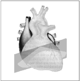
(a) 2-D echocardiography

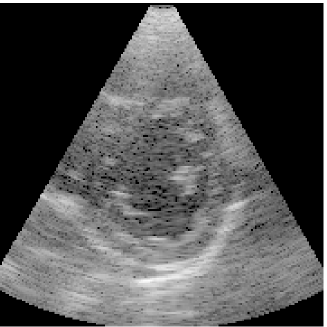
(b) Cross section of Left Ventricle

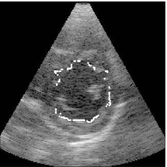
(c) Detected boundary points

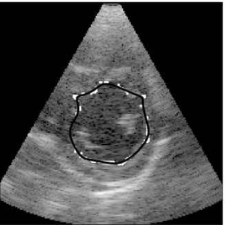
(d) Recovered boundary of LV computed by Algorithm 2

Fig. 4: The recovery of the boundary of the Left Ventricle from 2-D ultrasound images is a basic step in echocardiography to extract relevant parameters of cardiac function.

After having transformed the detected boundary points as described in (62)–(65) we can use Algorithm 2 to recover the boundary. The noise level $\delta$ depends on the technical equipment under use, it can be determined from experimental experience. Figure 5(a)–(b) demonstrate the importance of determining a proper degree for the approximating polynomial. The approximation displayed in Figure 5(a) has been computed by solving (1) where $M$ has been chosen too small, we obviously have underfitted the data. The overfitted approximation obtained by solving (1) using a too large $M$ is shown in Figure 5(b). The approximation shown in Figure 4(d) has been computed by Algorithm 2, it provides the optimal balance between fitting the data and smoothness of the solution.

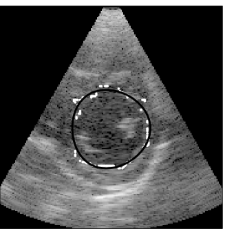
(a) Underfitted solution

(b) Overfitted solution

Fig. 5: The approximation in the left image results from using a too small polynomial degree, the approximation in the right image from a too large degree for the trigonometric approximation.

6.2 Boundary recovery from a sequence of images

In cardiac clinical studies one is more interested in the behavior of the Left Ventricle over a period of time rather than in a single “snapshot”. Thus for a fixed cross section we are given a sequence of ultrasound images (usually regularly spaced in time) describing the variation of the shape of the LV with time. One cycle from diastole (the state of maximal contraction of the LV), passing systole (the state of maximal expansion) to the next diastole consists typically of about 30 image frames. Since the behavior of the LV is (at least for a short period of time) almost periodic, one can model the varying shape of a fixed cross section of the LV as distorted two-dimensional torus, which in turn can be interpreted as 2-D trigonometric polynomial. Clearly we have to use a different degree for the time coordinate $\tau$ and for the spatial coordinate $u$.

Due to interfering biological structures and other distortions it sometimes happens that some of the image frames cannot be used to extract any reliable boundary information. Thus we have to approximate these missing boundaries from the information of the other image frames. To be more precise, assume that an echocardiographic examination provides a sequence of ultrasound images $I_{\tau}$ taken at time points $\tau=0,1,\dots,T-1$, where $T$ is approximately the length of one diastolic cycle (the time points could also be nonuniformly spaced). Assume that some of the images $I_{\tau}$ provide no useful information, so that we can only detect boundary points $\{s_{j,k}\}_{k=1}^{r_{j}}$ from the images $I_{\tau_{j}}$, where $\{\tau_{j}\}_{j=1}^{r}$ is a subset of $0,1,\dots T-1$. In order to get a complete description of the LV for the time interval $[0,T]$, we have not only to approximate the boundaries $f_{j}$ from each $I_{j}$, but we also have to recover the boundaries corresponding to the missing images. In other words we look for a 2-D trigonometric polynomial $p_{*}\in{{\boldsymbol{P}}^{2}_{\!M}}$ of appropriate degree $M$ that satisfies $p(\tau_{j},u_{j,k})\equiv(x_{j,k},y_{j,k})$ where the parameter $u$ is related to $s_{j,k}=x_{j,k}+iy_{j,k}$ by formulas (63)–(65). This approximation can be computed by the 2-D version of Algorithm 2, as indicated in the beginning of Section 5.

Under certain conditions we can use the 1-D version of Algorithm 2 instead of its 2-D version. As long as the assumptions of Corollary 8 are satisfied, we can compute $p_{*}\in{{\boldsymbol{P}}^{2}_{\!M}}$ by a successive application of Algorithm 2. We first approximate the boundaries $f_{j}$ for each $j$ separately from its samples $\{s_{j,k}\}_{k=1}^{r_{j}}$, which yields $j$ different polynomials $p^{(M_{j})}\in{{\boldsymbol{P}}_{\!M_{j}}}$. Having done this, the next step is to recover the missing boundaries at those time points where no information is available. We proceed by approximating successively the missing information “line by line”. We choose $u=0$, say, and approximate the missing information from the samples $p^{(M_{j})}(u)$ taken at the time points $\tau_{j},j=1,\dots,r$.

Note that the Toeplitz matrices of the systems $(T_{M})_{u}c^{(M)}_{u}=b^{(M)}_{u}$ coincide for all $u$, since the sampling geometry is constant along the $u$-coordinate (because we have recovered all samples at each $\tau_{j}$). Thus we have to solve multiple Toeplitz systems with the same system matrix but different right hand side. It is well-known that this can be done efficiently by exploiting the Gohberg-Semencul representation of the inverse of the Toeplitz matrix [14]. In our context this reads as follows. We solve

$$(T_{M})_{u}c^{(M)}_{u}=b^{(M)}_{u}$$ (66)

for one $u$ by Algorithm 2. We can solve now all other systems efficiently by establishing $(T_{M})^{-1}$ in the Gohberg-Semencul form

$$(T_{M})^{-1}=\left([L^{(M)}]^{\ast}L^{(M)}-U^{(M)}[U^{(M)}]^{\ast}\right)/z_{0}$$ (67)

where $L^{(M)}$ is a lower triangular Toeplitz matrix with $z=[z_{0},z_{1},\dots,z_{2M}]^{T}$ as its first column, $U^{(M)}$ is an upper triangular Toeplitz matrix with $[0,z_{1},\dots,z_{2M}]^{T}$ as its last column, $z$ being the first column of $(T_{M})^{-1}$. The matrix vector multiplications to compute $c^{(M)}_{u}=(T_{M})_{u}^{-1}b^{(M)}_{u}$ can now be carried out quickly using the Fast Fourier transform by embedding $L^{(M)}$ and $U^{(M)}$ into circulant matrices.

7 Miscellaneous remarks

For sampling sets with large gaps it can happen that the system $T_{M}c^{(M)}=b^{(M)}$ gets ill-conditioned with increasing degree $M$ and therefore Algorithm 2 may become unstable [6]. In this case one can use a different, more robust approach, which however comes at higher computational costs [27]. We solve the system $T_{M}c^{(M)}=b^{(M)}$ iteratively, e.g. by the conjugate gradient method until a certain stopping criterion is satisfied at iteration $k$, say, yielding the solution $c^{(M)}_{k}$. We use this solution as initial guess at the next level $M+1$ by setting $c^{(M+1)}_{0}=[0\,\,(c^{(M)}_{k})^{T}\,\,0]^{T}$. The crucial point in this procedure is to find a stopping criterion that guarantees convergence of the iterates, see [27, 24] for more details.

The computation of the entries of the Toeplitz matrix in Section 6 involves the nodes $u_{j}$ which in this particular case depend on the (perturbed) samples $s_{j}$. Therefore not only the right hand side $b^{(M)}$, but also $T_{M}$ is subject to perturbations. Hence in principle one might use the concept of total least squares (see [12]) instead of a least squares approach. A detailed discussion of this modification is beyond the scope of this paper.

References

• [1] H. Akaike, Block Toeplitz matrix inversion, SIAM J. Appl. Math., 24 (1973), pp. 234–241.
• [2] G. Ammar and W. Gragg, Superfast solution of real positive definite Toeplitz systems, SIAM J. Matrix Anal. Appl., 9 (1988), pp. 61–76.
• [3] G. Beylkin, On the fast Fourier transform of functions with singularities, Appl. Comp. Harm. Anal., 2 (1995), pp. 363–381.
• [4] S. Boyd, L. El Ghaoui, E. Feron, and V. Balakrishnan, Linear matrix inequalities in system and control theory, SIAM, Philadelphia, PA, 1994.
• [5] R. Chan and M. Ng, Conjugate gradient methods for Toeplitz systems, SIAM Review, 38 (1996), pp. 427–482.
• [6] G. Cybenko, The numerical stability of the Levinson-Durbin algorithm for Toeplitz systems of equations, SIAM J. Sci. Statist. Comp., 1 (1980), pp. 303–3190.
• [7] C. Demeure, Fast QR factorization of Vandermonde matrices, Linear Algebra Appl., 122–124 (1989), pp. 165–194.
• [8] P. Dierckx, Curve and surface fitting with splines, Monographs on Numerical Analysis, Oxford University Press, 1993.
• [9] A. Dutt and V. Rokhlin, Fast Fourier transforms for nonequispaced data, SIAM J. Sci. Comp., 14 (1993), pp. 1368–1394.
• [10] H. Fassbender, On numerical methods for discrete least-squares approximation by trigonometric polynomials, Math. Comp., 66 (1997), pp. 719–741.
• [11] H. G. Feichtinger, K. Gröchenig, and T. Strohmer, Efficient numerical methods in non-uniform sampling theory, Numerische Mathematik, 69 (1995), pp. 423–440.
• [12] R. Fierro, G. Golub, P. Hansen, and D. O’Leary, Regularization by truncated total least squares, SIAM J. Sci. Comp., 18 (1997), pp. 1223–1241.
• [13] W. Gautschi, How (un)stable are Vandermonde systems?, in Asymptotic and computational analysis (Winnipeg, MB, 1989), Dekker, New York, 1990, pp. 193–210.
• [14] I. Gohberg and A. Semencul, On the inversion of finite Toeplitz matrices and their continuous analogs, Mat. Issled., 2 (1972), pp. 201–233.
• [15] G. Golub, M. Heath, and G. Wahba, Generalized cross-validation as a method for choosing a good ridge parameter, Technometrics, 21 (1979), pp. 215–223.
• [16] G. Golub and C. van Loan, Matrix Computations, Johns Hopkins, Baltimore, third ed., 1996.
• [17] K. Gröchenig, personal communication.
• [18]  , A discrete theory of irregular sampling, Linear Algebra Appl., 193 (1993), pp. 129–150.
• [19]  , Finite and infinite-dimensional models for non-uniform sampling, in SampTA - Sampling Theory and Applications, Aveiro, Portugal, 1997, pp. 285–290.
• [20] P. Hansen, Analysis of discrete ill-posed problems by means of the L-curve, SIAM Review, 34 (1992), pp. 561–680.
• [21] N. Levinson, The Wiener RMS (root-mean square) error criterion in filter design and prediction, J. Math. Phys., 25 (1947), pp. 261–278.
• [22] A. Newbery, Trigonometric interpolation and curve-fitting, Math. Comp., 24 (1970), pp. 869–876.
• [23] A. Okabe, B. Boots, and K. Sugihara, Spatial tessellations: concepts and applications of Voronoĭ diagrams, John Wiley & Sons Ltd., Chichester, 1992. With a foreword by D. G. Kendall.
• [24] M. Rauth and T. Strohmer, Smooth approximation of potential fields from noisy scattered data, Geophysics, 63 (1998), pp. 85–94.
• [25] L. Reichel, G. Ammar, and W. Gragg, Discrete least squares approximation by trigonometric polynomials, Math. Comp., 57 (1991), pp. 273–289.
• [26] W. Rudin, Fourier Analysis on Groups, Wiley Interscience, New York, 1976.
• [27] O. Scherzer and T. Strohmer, A multi–level algorithm for the solution of moment problems, Num.Funct.Anal.Opt., 19 (1998), pp. 353–375.
• [28] T. Strohmer, Computationally attractive reconstruction of band-limited images from irregular samples, IEEE Trans. Image Proc., 6 (1997), pp. 540–548.
• [29] M. Suessner, M. Budil, T. Strohmer, M. Greher, G. Porenta, and T. Binder, Contour detection using artifical neuronal network presegmention, in Proc. Computers in Cardiology, Vienna, 1995.
• [30] D. Wilson, E. Geiser, and J. Li, Feature extraction in 2-dimensional short-axis echocardiographic images, J. Math. Imag. Vision, 3 (1993), pp. 285–298.