Abstract

We study numerical methods for the solution of general linear moment problems, where the solution belongs to a family of nested subspaces of a Hilbert space. Multi-level algorithms, based on the conjugate gradient method and the Landweber–Richardson method are proposed that determine the “optimal” reconstruction level a posteriori from quantities that arise during the numerical calculations. As an important example we discuss the reconstruction of band-limited signals from irregularly spaced noisy samples, when the actual bandwidth of the signal is not available. Numerical examples show the usefulness of the proposed algorithms.

Keywords and Phrases: Moment problems, multi–level algorithms, Landweber Richardson method, conjugate gradient method, nonuniform sampling.

AMS Subject Classification: 44A60, 65J10, 65J20, 62D05, 42A15.

1 Introduction

We study numerical methods for the solution of a family of general linear moment problems

(1.1) $$\langle x,g^{N}_{j}\rangle=\mu_{j}\qquad j\in I$$

where $\{g_{j}^{N}\}_{j\in I}$ is a complete system in $X_{N}$ and $\{X_{N}\}_{j\in I}$ is a family of nested subspaces of a separable Hilbert space $X$. $\langle x,g_{j}^{N}\rangle$ denotes the $j$–th moment. We consider the problem of recovering $x$ from noisy observations of the moments $\mu_{j}+\delta_{j}$.

Most existing methods for moments problems require exact a priori information about the space $X_{N}$ to which $x$ belongs to [BG68, XN94, LM91]. In many applications however this knowledge is not available, often we only know that $x$ belongs to some space of a whole family of Hilbert spaces $X_{N}$.

An important example is the problem of reconstructing a band-limited signal $x$ from irregularly spaced, noisy samples $x(t_{j})+\delta_{j}$, without explicit knowledge on the bandwidth of $x$. In other words we know that $x$ belongs to a space of a family of band-limited functions $X_{N}$ (where $N$ represents the bandwidth), but we do not know to which one. Most reconstruction algorithms require the a priori information of the actual bandwidth of $x$ (or at least a very good estimate) to be applicable. In numerical reconstructions overestimating the bandwidth of $x$ may result in a highly oscillating function, due to the noise in the samples. Underestimating the bandwidth may give a poor approximation to the original signal. From this point of view a proper choice of the level $N$ can also be seen as a regularization procedure.

For the numerical solution of the family of general moment problems we propose a multi–level approach that determines an “optimal” level $N$ a–posteriori from quantities that arise during the numerical calculations. The proposed algorithm does not use a–priori information on the level $N$ of the solution – all information required in the analysis of this algorithm is that there exists a level (bandwidth) $N_{*}$ such that the solution $x$ of (1.1) satisfies $x_{*}\in X_{N_{*}}$.

The outline of this paper is the following: In Section 2 and Section 3 we study multi–level algorithms for the efficient stable solution of moment problems. In particular we concentrate on a multi-level conjugate gradient algorithm and a multi-level Landweber–Richardson algorithm. These algorithms are formulated in a general setting. In Section 4 several applications to the numerical solution of moment problems are given, with the emphasize on reproducing kernel Hilbert spaces. In Section 5 we demonstrate in detail how the proposed algorithms can be applied to the problem of reconstructing a band-limited signal of unknown bandwidth from noisy irregularly spaced samples. Finally in Section 6 we demonstrate the performance of the multi-level algorithms by some numerical examples.

2 A multi–level algorithm based on the conjugate gradient method

In this section we introduce a multi–level algorithm based on the conjugate gradient for the numerical solution of moment problems. In this algorithm the levels are adapted inductively and at each level a conjugate gradient method is implemented.

In order to make the paper self–contained we outline the conjugate gradient method for the solution of linear systems: Let $T:X\to Y$ be a linear operator between separable Hilbert spaces $X$ and $Y$. By $T^{*}$ we denote the adjoint of the operator $T$. One efficient method for the solution of $Tx=y$ is the conjugate gradient method applied to the normal equation $T^{*}xT=T^{*}y$. This method, which is denoted by CGNE in the literature, is defined as follows (see e.g. [Han95, Han96, EHN96])

$$\framebox{$\begin{array}[]{l}\begin{array}[]{rcl}x_{0}&=&0\\ r_{0}&=&y\\ w_{0}&=&y\\ k&=&0\end{array}\\ \mbox{ repeat }\\ \left\{\begin{array}[]{rcl}d_{k}&=&T^{*}w_{k}\\ \alpha_{k}&=&\|T^{*}r_{k}\|^{2}/\|Td_{k}\|^{2}\\ x_{k+1}&=&x_{k}+\alpha_{k}d_{k}\\ r_{k+1}&=&r_{k}-\alpha_{k}Td_{k}\\ \beta_{k}&=&\|T^{*}r_{k+1}\|^{2}/\|T^{*}r_{k}\|^{2}\\ w_{k+1}&=&r_{k+1}+\beta_{k}w_{k}\\ k&=&k+1\\ \end{array}\right.\\ \mbox{ until }\|r_{k}\|<\rho\|y\|\end{array}$}$$

Before we study a multi–level scheme based on the CGNE method we introduce some notation:

Assumption 2.1

$\{X_{N}\}_{N\in\mbox{\myfontsmall N}_{0}}$ is a family of linearly ordered subspaces of a separable Hilbert space $X$. For $N\in\mbox{\myfontsmall N}_{0}$ let $P_{N}$ be the orthogonal projectors from $X$ into $X_{N}$ and let ${\cal R}(T_{N}^{*})$ denote the range of $T_{N}^{*}$. For $N\in\mbox{\myfontsmall N}_{0}$ the family of linear operators $T_{N}:X_{N}\to Y$ satisfies

(2.7) $$\left\{\begin{array}[]{cl}\mbox{\em(i)}&\,\,\,\|T_{N}\|\leq 1\,,\\ \mbox{\em(ii)}&\,\,\,T_{N}x_{M}=T_{M}x_{M}\mbox{ for all }N\geq M\,,\\ \mbox{\em(iii)}&\,\,\,{\cal{R}}(T_{N}^{*})\subseteq X_{N}\,.\end{array}\right.$$

The first assumption in (2.7) is that the operators $T_{N}$ are properly scaled. The second assumption is that on subspaces of level $M(<N)$ the operators $T_{M}$ and $T_{N}$ coincide. The third assumptions guarantees that the iterates of the CGNE method are contained in $X_{N}$.

For given data $y\in Y$ we are concerned with finding $N\in\mbox{\myfontsmall N}_{0}$ and $x\in X_{N}$, which satisfy

(2.8) $$T_{N}x=y{\;}.$$

The terminology of a solution of (2.8) is well–defined by Assumption (2.1), since from this it follows that a solution on a lower scale is also a solution on a higher scale.

In the sequel we will assume that there exists a solution of (2.8).

Assumption 2.2

There exists $N_{*}\in\mbox{\myfontsmall N}_{0}$ and $x_{*}\in X_{N_{*}}$ which satisfy (2.8).

We note that we do not assume the knowledge of $N_{*}$. If for instance $X_{N}$ denotes the Payley–Wiener space of band-limited functions of bandwidth less or equal $N$ and $N\to\infty$, then the meaning of Assumption 2.2 is: There exists a band-limited function which solves (2.8).

By $y^{\delta}\in Y$ we denote measured data of $y$, which satisfies

(2.9) $$\|y^{\delta}-y\|\leq\delta{\;}.$$

Algorithm 2.3

Let $\eta>0$, $\tau>1$.

At level $0:$ Without loss of generality we assume that $x_{0,0}^{\delta}\in X_{0}$ satisfies

1. $\|T_{0}(x_{0,0}^{\delta})-y^{\delta}\|^{2}>2(1+\eta)\left(\delta+\|P_{0}x_{*}-x_{*}\|\right)\|y^{\delta}\|$,

2. $\|T_{0}(x_{0,0}^{\delta})-y^{\delta}\|^{2}>2(1+\eta)\tau\delta\|y^{\delta}\|$.

If 2. does not hold, then $x_{0,0}^{\delta}$ is accepted as an approximate solution and the multi–level algorithm is terminated. If 1. does not hold, but 2. is satisfied, then we can choose a level $J$ such that

$$\|T_{J}(x_{0,0}^{\delta})-y^{\delta}\|^{2}=\|T_{0}(x_{0,0}^{\delta})-y^{\delta}\|^{2}>2(1+\eta)\left(\delta+\|P_{J}x_{*}-x_{*}\|\right)\|y^{\delta}\|{\;}.$$

In this situation we simply renumber the levels and make the setting $0=J$. For the new setting $J=0$ both 1. and 2. hold, and the CGNE method at level $0$ is performed. The iteration at scale $X_{0}$ is terminated if for the first time

$$\|T_{0}(x_{k+1,0}^{\delta})-y^{\delta}\|^{2}\leq 2(1+\eta)\left(\delta+\|P_{0}x_{*}-x_{*}\|\right)\|y^{\delta}\|{\;}.$$

The termination index is denoted by $k=k_{*}(0,\delta)$.

From level $N$ to level $N+1$: If $\|T_{N+1}(x_{k_{*}(N,\delta)+1,N}^{\delta})-y^{\delta}\|^{2}\leq 2(1+\eta)\tau\delta\|y^{\delta}\|$, then the multi–level algorithm terminates and $x_{k_{*}(N,\delta)+1,N}^{\delta}$ is an approximate solution. Else we define $x_{k_{*}(N,\delta),N}^{\delta}=:x_{0,N+1}^{\delta}$. Since $\|P_{N+1}x_{*}-x_{*}\|\leq\|P_{N}x_{*}-x_{*}\|$ it follows from the definition of $k_{*}(N,\delta)$:

$$\|T_{N+1}(x_{0,N+1}^{\delta})-y^{\delta}\|>2(1+\eta)\left(\delta+\|P_{N+1}x_{*}-x_{*}\|\right)\|y^{\delta}\|{\;}.$$

Therefore, at least one iteration of CGNE at level $N+1$ is performed. The iteration at scale $X_{N+1}$ is terminated if

$$\|T_{N+1}(x_{k+1,N+1}^{\delta})-y^{\delta}\|^{2}\leq 2(1+\eta)\left(\delta+\|P_{N+1}x_{*}-x_{*}\|\right)\|y^{\delta}\|$$

for the first time. The termination index is denoted by $k=k_{*}(N+1,\delta)$.

The idea of using multi–level algorithms as considered in this paper for the solution of ill–posed problems has been considered in [Sch96].

In the following, we verify some basic monotonicity properties of the iterates of the multi–level algorithm 2.3. Note that in practice when the CGNE–method is used for solving linear systems the CGNE method is usually terminated with a discrepancy principle (see e.g. [Han96]). Hanke [Han96] showed by a counterexample that in general the error of the iterates of the CGNE method does not monotonically decrease when the iteration is terminated by the discrepancy principle. In this paper the CGNE–method is combined with a multi–level algorithm and we expect that a reasonable performance of this method is depending on providing a good initially guess for starting the CGNE method at a higher level. Therefore, we concentrate in this paper on a stopping criterion, which guarantees monotonicity of the iterates at each level.

Proposition 2.4

Let assumption 2.1 hold, and let the iteration at fixed level $N$ be stopped according to the generalized discrepancy principle

(2.10) $$\|T_{N}(x_{k,N}^{\delta})-y^{\delta}\|^{2}>2(1+\eta)\left(\delta+\|P_{N}x_{*}-x_{*}\|\right)\|y^{\delta}\|\,\mbox{ for }0\leq k\leq k_{*}(N,\delta){\;}.$$

Then $k_{*}(N,\delta)<\infty$ and

$$\begin{array}[]{rclr}\|x_{j+1}^{N}-P_{N}x_{*}\|&\leq&\|x_{j}^{N}-P_{N}x_{*}\|&\quad j=0,...,k_{*}(N,\delta)\,,\\ \|x_{j+1}^{N}-x_{*}\|&\leq&\|x_{j}^{N}-x_{*}\|&\quad j=0,...,k_{*}(N,\delta)\;.\end{array}$$

Proof: Application of the general results in [Han96] immediately yields $k_{*}(N,\delta)<\infty$ and for $j=0,...,k_{*}(N,\delta)$ $\|x_{j+1}^{N}-x_{*}\|\leq\|x_{j}^{N}-x_{*}\|$. Therefore we have

$$\|x_{j+1}^{N}-P^{N}x_{*}\|^{2}+2\langle x_{j+1}^{N}-P^{N}x_{*},P^{N}x_{*}-x_{*}\rangle\leq\|x_{j}^{N}-x_{*}\|^{2}+\langle x_{j+1}^{N}-P^{N}x_{*},P^{N}x_{*}-x_{*}\rangle.$$

From the remark following Assumption 2.1 it follows $x_{j}^{N},x_{j+1}^{N}\in X_{N}$ and therefore the assertion is proven. $\Box$

From Proposition 2.4 it follows that (2.10) determines a well–defined stopping index for the CGNE method at level $N$.

2.1 Convergence and stability of the multi–level algorithm

Using the monotonicity results of the iterates of the multi–level schemes we prove below that the multi–level scheme is convergent and stable. The following lemma will be central for our further considerations.

Lemma 2.5

Let $\delta=0$. If Assumptions 2.1 and 2.2 holds, then the multi–level algorithm 2.3

terminates after a finite number of iterations

or

there exists a level $\hat{N}$ such that at each level $N<\hat{N}$ a finite number of CGNE–iterations are performed and at level $\hat{N}$ the CGNE iteration does not terminate.

Proof: If $\delta=0$, then the stopping criterion (2.10) for the CGNE method at level $N$ is

(2.12) $$\|T_{N}(x_{k,N}^{\delta})-y\|^{2}>2(1+\eta)\|P_{N}x_{*}-x_{*}\|\|y\|\mbox{ for }0\leq k\leq k_{*}(N,0){\;}.$$

If $\delta=0$, then the stopping criterion for the multi–level algorithm is

(2.13) $$\|T_{N}(x_{k,N}^{\delta})-y\|=0{\;}.$$

Let $\hat{N}$ be the first level–index where $P_{N}x_{*}=x_{*}$. A finite level–index exists by Assumption 2.2. From Proposition 2.4 it follows that for each level $N<\hat{N}$ the number of iterations of the CGNE method is finite, which yields the assertion. $\Box$

Using the previous lemma, we are able to prove that the multi–level CGNE algorithm is convergent in the case of exact data.

Theorem 2.6

Let Assumption 2.2 hold. Then the multi–level CGNE algorithm converges to a solution $\hat{x}$.

Proof: Let $\hat{N}$ be the smallest index $N$ such that $P_{N}x_{*}=x_{*}$. We differ between two cases:

1. The multi–level CGNE method terminates at level $\hat{N}$ after a finite number of iterations

2. The multi–level CGNE method does not terminate

In the first case it follows from (2.13) that the last iterate $\hat{x}$ satisfies $T_{\hat{N}}^{*}\hat{x}=y\;,$ which shows that $\hat{x}$ is the solution.
In the second case it follows immediately from Theorem 3.4 in [Han95] that $x_{n}$ is convergent to a solution. $\Box$

In the case of perturbed data, it follows from Proposition 2.4 that the discrepancy principle (2.10) determines a well–defined (finite) stopping index at level $N<\hat{N}$, which is denoted by $k_{*}(N,\delta)$. In the following, we will assume that the multi–level algorithm is finally terminated if for the first time

(2.14) $$\|T_{N}(x_{k,N}^{\delta})-y^{\delta}\|^{2}\leq 2(1+\eta)\tau\delta\|y^{\delta}\|{\;}.$$

From Lemma 2.5 and Assumption 2.2 it follows that this criterion determines a well–defined stopping index at level $N(\delta)$, which is denoted by $K_{*}(N(\delta),\delta)$.

Our next result shows that the multi–level iteration is a stable method.

Theorem 2.7

Let the assumptions of Theorem 2.6 hold and assume that $T_{N_{*}}$ is continuously invertible (here $N_{*}$ is as introduced in Assumption 2.2). If $y^{\delta}$ fulfills (2.9), and if the iteration at level $N$ is stopped according to the discrepancy principle (2.10), and the multi–level iteration is terminated by (2.14), then

$$x_{N_{n},K_{*}(N_{n},\delta)}^{\delta}\to x_{*},\qquad\delta\to 0{\;}.$$

Proof: Let $\delta_{n}$, $n=1,2,...,$ be a sequence converging to zero as $n\to\infty$, and let $y_{n}:=y^{\delta_{n}}$ be a corresponding sequence of perturbed data. For each pair $(\delta_{n},y_{n})$, denote by $K_{n}=K_{*}(N(\delta_{n}),\delta_{n})$ the corresponding stopping index at termination level $N_{n}=N(\delta_{n})$ determined by (2.14). A comparison of $\delta_{n}+\|P_{N(\delta_{n})}x_{*}-x_{*}\|$ and $\tau\delta_{n}$ shows that $N(\delta_{n})\leq N_{*}$. From Proposition 2.4 and the results in [Han96] it follows that for $0\leq k\leq k_{*}(N,\delta)$ and $0\leq N\leq N_{*}$

$$\|x_{k,N}^{\delta}-x_{*}\|\leq\|x_{0,0}^{\delta}-x_{*}\|\mbox{ and }\|T_{N_{*}}x_{k,N}^{\delta}-y\|\to 0\,.$$

From the continuous invertibility of $T_{N_{*}}$ the assertion follows. $\Box$

3 A multi–level algorithm based on the Landweber–Richardson method

As an alternative to the multi–level algorithm based on CGNE we study in this section a multi–level iteration based on the Landweber–Richardson method for solving moment problems. It will turn out that different stopping criteria can be used for stopping the Landweber–Richardson method than for the CGNE method.

The multi–level iteration based on the Landweber–Richardson method is defined as follows

Algorithm 3.1

Let $\eta>0$, $\tau>1$.

At level $0:$ Without loss of generality we assume that $x_{0,0}^{\delta}\in X_{0}$ satisfies

1. $\|T_{0}(x_{0,0}^{\delta})-y^{\delta}\|>2(1+\eta)\left(\delta+\|P_{0}x_{*}-x_{*}\|\right)$,

2. $\|T_{0}(x_{0,0}^{\delta})-y^{\delta}\|>2(1+\eta)\tau\delta$.

If 2. does not hold, then $x_{0,0}^{\delta}$ is accepted as an approximate solution and the multi–level algorithm is terminated. If 1. does not hold, but 2. is satisfied, then we can choose a level $J$ such that

$$\|T_{J}(x_{0,0}^{\delta})-y^{\delta}\|=\|T_{0}(x_{0,0}^{\delta})-y^{\delta}\|>2(1+\eta)\left(\delta+\|P_{J}x_{*}-x_{*}\|\right){\;}.$$

In this situation we simply renumber the levels and set $0=J$. With the new setting both 1. and 2. hold, and the “Landweber–Richardson” iteration at level $0$ is performed

$$x_{k+1,0}^{\delta}=x_{k,0}^{\delta}-T_{0}^{*}\left(T_{0}(x_{k,0}^{\delta})-y^{\delta}\right){\;}.$$

The iteration at scale $X_{0}$ is terminated if for the first time

$$\|T_{0}(x_{k+1,0}^{\delta})-y^{\delta}\|\leq 2(1+\eta)\left(\delta+\|P_{0}x_{*}-x_{*}\|\right){\;}.$$

The termination index is denoted by $l_{*}(0,\delta)$.

From level $N$ to level $N+1$: If $\|T_{N+1}(x_{l_{*}(N,\delta)+1,N}^{\delta})-y^{\delta}\|\leq 2(1+\eta)\tau\delta$, then the multi–level algorithm terminates and $x_{l_{*}(N,\delta)+1,N}^{\delta}$ is an approximate solution. Else we define $x_{l_{*}(N,\delta),N}^{\delta}=:x_{0,N+1}^{\delta}$. Since $\|P_{N+1}x_{*}-x_{*}\|\leq\|P_{N}x_{*}-x_{*}\|$ it follows from the definition of $l_{*}(N,\delta)$:

$$\|T_{N+1}(x_{0,N+1}^{\delta})-y^{\delta}\|>2(1+\eta)\left(\delta+\|P_{N+1}x_{*}-x_{*}\|\right){\;}.$$

Therefore, at least one iteration of Landweber–Richardson method at level $N+1$ is performed and

$$x_{k+1,N+1}^{\delta}=x_{k,N+1}^{\delta}-T_{N+1}^{*}\left(T_{N+1}(x_{k,N+1}^{\delta})-y^{\delta}\right){\;}.$$

The iteration at scale $X_{N+1}$ is terminated if

$$\|T_{N+1}(x_{k+1,N+1}^{\delta})-y^{\delta}\|\leq 2(1+\eta)\left(\delta+\|P_{N+1}x_{*}-x_{*}\|\right)$$

for the first time. The termination index is denoted by $l_{*}(N+1,\delta)$.

In the following, we verify some basic monotonicity properties of the iterates of the multi–level algorithm 3.1.

Proposition 3.2

Let Assumptions 2.1 and 2.2 hold. At fixed level $N$ let the iteration be stopped according to the generalized discrepancy principle

(3.1) $$\|T_{N}(x_{k,N}^{\delta})-y^{\delta}\|>2(1+\eta)\left(\delta+\|P_{N}x_{*}-x_{*}\|\right)\,\mbox{ for }0\leq k\leq l_{*}(N,\delta){\;}.$$

Then

(3.2) $$\|x_{j+1}^{N}-P_{N}x_{*}\|\leq\|x_{j}^{N}-P_{N}x_{*}\|\quad j=0,...,l_{*}(N,\delta)\;.$$

Moreover, if (3.1) at level $N+1$ does not become active for $x_{0,N+1}^{\delta}$, then

(3.3) $$\|x_{1,N+1}^{\delta}-x_{*}\|^{2}\leq\|x_{0,N+1}^{\delta}-x_{*}\|^{2}-\frac{\eta}{1+\eta}\|T_{N}x_{0,N+1}^{\delta}-y^{\delta}\|^{2}{\;}.$$

Proof: From the definition of the multi–level Landweber–Richardson method it follows

(3.9) $$\begin{array}[]{rcl}\displaystyle\|x_{k+1,N}^{\delta}-P_{N}x_{*}\|^{2}&=&\displaystyle\|x_{k,N}^{\delta}-P_{N}x_{*}\|^{2}+\|T_{N}^{*}(T_{N}(x_{k,N}^{\delta})-y^{\delta})\|^{2}\\ &&\displaystyle-2\langle T_{N}(x_{k,N}^{\delta}-P_{N}x_{*}),T_{N}(x_{k,N}^{\delta})-y^{\delta}\rangle\\ &=&\displaystyle\|x_{k,N}^{\delta}-P_{N}x_{*}\|^{2}-2\|T_{N}(x_{k,N}^{\delta})-y^{\delta}\|^{2}\\ &&\displaystyle+\|T_{N}^{*}\left(T_{N}(x_{k,N}^{\delta})-y^{\delta}\right)\|^{2}\\ &&\displaystyle+2\langle T_{N}(P_{N}x_{*})-y^{\delta},T_{N}(x_{k,N}^{\delta})-y^{\delta}\rangle\;.\end{array}$$

From (3.1) and (2.8) it follows

(3.12) $$\begin{array}[]{rcl}\|T_{N}(P_{N}x_{*})-y^{\delta}\|&\leq&\delta+\|T_{N_{*}}(P_{N}x_{*})-T_{N_{*}}(x_{*})\|\\ &\leq&\delta+\|P_{N}x_{*}-x_{*}\|{\;}.\end{array}$$

For $0\leq k\leq l_{*}(N,\delta)$ it follows from (2.7), (3.9) and (3.12) that

(3.16) $$\begin{array}[]{rcl}\displaystyle\|x_{k+1,N}^{\delta}-P_{N}x_{*}\|^{2}&\leq&\displaystyle\|x_{k,N}^{\delta}-P_{N}x_{*}\|^{2}-\|T_{N}(x_{k,N}^{\delta})-y^{\delta}\|^{2}\\ &&\displaystyle+2\|T_{N}(P_{N}x_{*})-y^{\delta}\|\|T_{N}(x_{k,N}^{\delta})-y^{\delta}\|\\ &\leq&\displaystyle\|x_{k,N}^{\delta}-P_{N}x_{*}\|^{2}-\frac{\eta}{1+\eta}\|T_{N}(x_{k,N}^{\delta})-y^{\delta}\|^{2}\;.\end{array}$$

Now (3.2) can be easily proven with an inductive argument. (3.3) can be proven with similar arguments as above.   $\Box$

From Proposition 3.2 it follows that (3.1) determines a well–defined stopping index for the Landweber–Richardson method at level $N$.

Corollary 3.3

Let Assumptions 2.1 and 2.2 hold. Let the Landweber–Richardson iteration at fixed level $N$ be stopped according to the generalized discrepancy principle (3.1). If

(3.17) $$\delta+\|P_{N}x_{*}-x_{*}\|>0\,,$$

then

$$l_{*}(N,\delta)<\infty\;.$$

Proof: From (3.1) and (3.16) it follows

$$\begin{array}[]{rcl}\displaystyle 4\eta(1+\eta)\sum_{k=0}^{l_{*}(N,\delta)}\left(\delta+\|P_{N}x_{*}-x_{*}\|\right)^{2}&\leq&\displaystyle\|x_{l_{*}(N,\delta)+1,N}^{\delta}-P_{N}x_{*}\|^{2}\\ &&\displaystyle+\frac{\eta}{1+\eta}\sum_{k=0}^{l_{*}(N,\delta)}\|T_{N}(x_{k,N}^{\delta})-y^{\delta}\|^{2}\\ &\leq&\displaystyle\|x_{0,N}^{\delta}-P_{N}x_{*}\|^{2}\\ &<&\displaystyle\infty\,.\end{array}$$

This together with (3.17) shows $l_{*}(N,\delta)<\infty$. $\Box$

So far we have proven a monotonicity result for the iterates of the Landweber–Richardson method at fixed level $N$. In the following we show that the iterates of the multi–level algorithm also satisfy a certain monotonicity when the levels are switched. This together with Proposition 3.2 provides monotonicity of the iterates of the multi–level algorithm 3.1.

3.1 Convergence and stability of the multi–level algorithm

Using the monotonicity results of the iterates of the multi–level schemes based on the Landweber–Richardson method we verify below that the multi–level scheme is convergent and stable. The following lemma will be central for our further considerations. The proof of this lemma is analogous to the proof of Lemma 2.5.

Lemma 3.4

Let $\delta=0$. If Assumptions 2.1 and 2.2 hold, the multi–level algorithm 3.1

terminates after a finite number of iterations

or

there exists a level $\hat{N}$ such that at each level $N<\hat{N}$ a finite number of Landweber–Richardson iterations are performed and at level $\hat{N}$ the Landweber–Richardson iteration does not terminate.

Similarily as in Section 2 (using instead of Hanke’s results in the proof of Theorem 2.6 some well–known results on convergence properties of the Landweber–Richardson method (see e.g. Groetsch [Gro84]) it is possible to prove that the multi–level Landweber–Richardson algorithm is convergent in the case of exact data.

Theorem 3.5

Let Assumptions 2.1 and 2.2 hold. Then the multi–level Landweber–Richardson algorithm converges to a solution $\hat{x}$.

In the case of perturbed data, it follows from Corollary 3.3 that the discrepancy principle (3.1) determines a well–defined (finite) stopping index at level $N<\hat{N}$, which is denoted by $l_{*}(N,\delta)$. In the following we finally terminate the multi–level algorithm if for the first time

(3.19) $$\|T_{N}(x_{k,N}^{\delta})-y^{\delta}\|\leq 2(1+\eta)\tau\delta{\;}.$$

From Corollary 3.3 and Assumption 2.2 it follows that this criterion determines a well–defined stopping index at level $N(\delta)$, which is denoted by $L_{*}(N(\delta),\delta)$.

Our next result shows that the multi–level iteration is a stable method. The proof of this result is analogous to the proof of Theorem 2.7

Theorem 3.6

Let the assumptions of Theorem 3.5 hold and assume that $T_{N_{*}}^{*}$ is continuously invertible. If $y^{\delta}$ fulfills (2.9), and if the iteration at level $N$ is stopped according to the discrepancy principle (3.1), and the multi–level iteration is terminated by (3.19), then

$$x_{N(\delta),L_{*}(N(\delta),\delta)}^{\delta}\to x_{*},\qquad\delta\to 0{\;}.$$

In practical applications, if the quantity $\|P^{N}x_{*}-x_{*}\|$ is substantially underestimated, it may happen that the algorithm does not switch to the next level although the iterations stagnate and the approximations do not improve significantly any more. This can be avoided for the multi–level iteration based on Landweber–Richardson method by using alternatively the following stopping criterion:

(3.20) $$\|x_{k+1}^{N}-x_{k}^{N}\|>2(1+\eta)\tau\delta\mbox{ for }k=0,...,\hat{l}_{*}(N,\delta){\;}.$$

Then, from the definition of the Landweber–Richardson method it follows under the Assumption 2.1

$$\|(T_{N}x_{N}-y^{\delta})\|\geq\|T_{N}^{*}(T_{N}x_{N}-y^{\delta})\|=\|x_{k+1}^{N}-x_{k}^{N}\|>2(1+\eta)\tau\delta{\;}.$$

Therefore we have $l_{*}(N,\delta)\geq\hat{l}_{*}(N,\delta)$. From this it is obvious to see that Proposition 3.2, Corollary 3.3, Lemma 3.4 and Theorem 3.5 are valid, if we replace in these results $l_{*}$ by $\hat{l}_{*}$. It is also quite easy to see that (3.20) determines a well–defined stopping criterion. The proof of Theorem 3.5 for the multi–level Landweber–Richardson method with the stopping criterion 3.20 requires the assumption that $T_{N_{*}}^{*}$ is continuously invertible to guarantee that the solution of $T_{N_{*}}^{*}x=y$ is a solution of $T_{N_{*}}(T_{N_{*}}^{*}-y)=0$ and vice versa.

4 The multi–level algorithm for the moment problem

In the sequel we show the multi-level algorithms 2.3 and 3.1 can be applied for the solution of general moment problems as described in Section 1.

It is well-known that a signal $x\in X_{N}$ can be completely reconstructed from its moments $\langle x,g_{j}^{N}\rangle$ if the set $\{g_{j}^{N}\}_{j\in I}$ is a frame for $X_{N}$. For the readers convenience we quote the definition of a frame (see e.g. [You80]):

Definition 4.1

A family $\{g_{j}^{N}\}_{j\in I}$ is a called a frame for $X_{N}$ if there exist constants $A_{N},B_{N}$, called the frame bounds, such that

(4.21) $$A_{N}\|x\|^{2}\leq\sum_{j\in I}|\langle x,g^{N}_{j}\rangle|^{2}\leq B_{N}\|x\|^{2}\quad\forall x\in X_{N}\,.$$

In this paper (if not stated otherwise) we will always assume that the family $\{g^{N}_{j}\}_{j\in I}$ is a frame for $X_{N}$. For a given frame $\{g^{N}_{j}\}_{j\in I}$ we introduce the following linear operator

(4.22) $$T_{N}:X_{N}\rightarrow\ell^{2}(I)\,,\qquad T_{N}x=\{\langle x,g^{N}_{j}\rangle\}_{j\in I}{\;}.$$

The operator $T_{N}$ satisfies $\|T_{N}\|\leq\sqrt{B_{N}}$. The adjoint operator is given by

(4.23) $$T_{N}^{*}:\ell^{2}(I)\rightarrow X_{N},\qquad T_{N}^{*}\{\mu_{j}\}_{j\in I}=\sum_{j\in I}\mu_{j}g^{N}_{j}\,.$$

We note that if the family $\{g^{N}_{j}\}_{j\in J}$ is an orthonormal basis on $X_{N}$, then $T_{N}$ is a unitary operator and $T_{N}^{*}=(T_{N})^{-1}$.

As usual we define the frame operator by

(4.24) $$S_{N}:X_{N}\rightarrow X_{N},\qquad S_{N}x=T_{N}^{*}T_{N}x=\sum_{j\in I}\langle x,g^{N}_{j}\rangle g^{N}_{j}\,.$$

It is well–known that $S_{N}$ is positive definite and invertible if $\{g_{j}^{N}\}_{j\in J}$ is a frame. Stability results for frames in conjunction with moment problems can be found in [Chr96].

Obviously the operator $T_{N}$ (respectively the scaled operator $\frac{1}{\sqrt{B}}T$) satisfies Assumption 2.7(i) and (iii). A sufficient (but not necessary) condition for the frame analysis operators $T_{N}$ to satisfy Assumption 2.7(ii) is for instance when the frame elements $g^{N}_{j}$ correspond to reproducing kernels, see Section 4.1 below. With the notation introduced above this shows the setting in which the generally defined multi-level algorithms of Section 2 and Section 3 can be applied to recover $x$ from noisy moment measurements $y^{\delta}=\{\langle x,g_{j}^{N}\rangle+\delta_{j}\}_{j\in I}$.

For practical applications many delicate problems have to be solved before implementation of the multi level algorithms. We need conditions which allow an easy verification that the set $\{g_{j}^{N}\}$ is a frame for $X_{N}$, as well as useful estimates of the frame bounds. And finally we have to find appropriate estimates for $\|P_{N}x_{*}-x_{*}\|$ occurring in the stopping criteria  (2.10) and (3.1).

In Section 5 we summarize recent results from the literature which allow to estimate frame bounds efficiently.

4.1 Signal recovery in reproducing kernel Hilbert spaces

A special case of the moment problem occurs in reproducing kernel Hilbert spaces. Let $X$ be a Hilbert space of real or complex valued functions defined on a subset $I$ of ℝ with inner product $\langle\cdot,\cdot\rangle$. We recall that a Hilbert space $X$ is called a reproducing kernel Hilbert space if for every element $t\in I$ the “point evaluation” $x\mapsto x(t)$ on $X$ is bounded. From the Riesz representation theorem it follows that there exists a unique $K_{t}\in X$, which satisfies

(4.25) $$\langle x,K_{t}\rangle=x(t)\quad\mbox{ for every }x\in X$$

The reproducing kernel $K$ on $I\times I$ is defined by

(4.26) $$K(t,u):=\langle K_{t},K_{u}\rangle=K_{t}(u){\;}.$$

In this section for application of the multi-level algorithm of Section 2 we use a family of reproducing kernel Hilbert spaces $X_{N}$. Note that every closed subspace of a RKHS is itself a RKHS. Thus a reproducing kernel Hilbert space always contains a family of nested reproducing kernel subspaces.

If $X_{N}\subseteq X$ is a RKHS, then the orthogonal projector of $X$ onto $X_{N}$ can be characterized by (see e.g. [Ist87, Chapter 11])

(4.27) $$(P_{X_{N}}x)(t)=\langle x,K^{N}_{t}\rangle{\;}.$$

The following lemma is an immediate consequence of the above characterization of the orthogonal projector $P_{N}$

Lemma 4.2

Let $x_{M}\in X_{M}$, where $M\geq N$. Moreover, let $T_{N}$ be defined by

$$T_{N}(\cdot):=\langle\cdot,g_{j}^{N}\rangle\,,$$

where $g_{j}^{N}=K^{N}(\cdot,j)$. Then

(4.28) $$T_{N}(P_{N}x_{M})=T_{N}x_{M}{\;}.$$

Using Lemma 4.2 we are able to verify the general assumptions in the convergence and stability results of the multi–level algorithm. Moreover, we discuss details of the numerical implementation, especially implementation of the stopping criteria.

For reproducing kernel Hilbert space the stopping criterion (3.1) is equivalent to

$$|\sum_{j\in I}x_{k,N}^{\delta}(t_{j})-y^{\delta}|\leq 2(1+\eta)\left(\delta+\|P_{N}x_{*}-x_{*}\|\right)\,.$$

There are several important examples of reproducing kernel Hilbert spaces which deserve to be mentioned explicitly.

(i) Let $x\in{\cal B}_{N}$ where ${\cal B}_{N}$ is the space of band-limited functions, i.e.

(4.29) $$\int_{-\infty}^{\infty}|x(t)|^{2}dt<\infty\,\,\mbox{ and }\,\,\mbox{supp\/}\,\hat{x}\subseteq[-N,N]\,,$$

where $\hat{x}$ denotes the Fourier transform of $x$. The space ${\cal B}_{N}$ is a RKHS with reproducing kernel

(4.30) $$K^{N}(t,u)=\frac{\sin N(t-u)}{N(t-u)}\,.$$

This space is of paramount importance for digital signal processing, see e.g. [Hig96]. We will deal with ${\cal B}_{N}$ in more detail in Section 5 in conjunction with signal recovery and bandwidth estimation from nonuniformly spaced noisy samples.

(ii) The RKHS ${\cal P}_{N}$ consists of all trigonometric polynomials $p$ of degree $N$ given by

(4.31) $$p(t)=\sum_{n=-N}^{N}a_{n}e^{2\pi int}\,.$$

The reproducing kernel is $K(t,u)=D_{N}(t-u)$ where the Dirichlet kernel is

(4.32) $$D_{N}(t)=\frac{\sin\,(2N+1)\pi t}{\sin\,\pi t}\,.$$

It follows immediately from the fundamental theorem of algebra that the set $\{g_{j}\}_{j\in I}$, where $g_{j}(t)=D_{N}(t-t_{j})$ constitutes a frame for ${\cal P}_{N}$ whenever $|I|>2N$, where the sampling points $t_{j}$ may be randomly spaced. Gröchenig has derived estimates of the frame bounds for the weighted frame $\{w_{j}g_{j}\}_{j\in I}$, if the maximal gap between two successive sampling points satisfies a certain criterion, see [Gro93].

(iii) Sobolev spaces $H^{r}$ for $r>\frac{1}{2}$ are well known to possess reproducing kernels. Note however that the inner product on $H^{r}$ is not the restriction of that of $L^{2}(\mbox{\myfontsmall R})$. Hence the formulae in the previous sections must be reinterpreted in terms of the $H^{r}$ inner product. See [NW91] for a detailed discussion of Sobolev spaces and reproducing kernels.

Wavelet subspaces that constitute a so-called multiresolution analysis (MRA) [Mal89, Dau92] are further important examples for reproducing kernel Hilbert spaces [XN94], where moment problems arise naturally when one wants to reconstruct a function from its wavelet coefficients. Recently the concept of a MRA has been generalized, leading to a so-called frame multiresolution analysis [BL97]. More examples for reproducing kernel Hilbert spaces can be found in [NW91, Ist87].

5 Reconstructing a signal of unknown bandwidth from irregularly spaced noisy samples

In many practical applications, for instance in geophysics, spectroscopy, medical imaging, the signal cannot be sampled at regularly spaced points. Thus one is confronted with the problem of reconstructing an irregularly sampled signal. Often the signal can be assumed to be band-limited (or at least essentially band-limited), but the actual bandwidth is not known.

The problem of reconstructing a band-limited signal $x$ from regularly and irregularly samples $\{x(t_{j})\}_{j\in I}$ has attracted many mathematicians and engineers. Many theoretical results and efficient algorithms have been derived in the last years, see e.g. [Zay93, FG94, Sam95, Hig96] and the references cited therein. In [Chr96] results on frame perturbations are applied to the irregular sampling problem to derive error estimates for the approximation. Most of these results are based on the assumption that the bandwidth of the signal to be recovered is known a priori. However in many applications this assumption is not justified. This is the motivation to consider the problem of reconstructing a band-limited signal whose actual band-width is not known, given only a set of nonuniformly located and noisy samples.

In the sequel we show that the multi-level algorithm developed in Section 2 in combination with the results of Section 4 provides an efficient solution to this problem. To do this, we verify the general assumptions in the convergence and stability results of the multi–level algorithm.

In the approach suggested below, we use the adaptive weights method developed by Feichtinger and Gröchenig [FG94]. The adaptive weights method is based on the fact that a signal $x\in{\cal B}_{N}$ can be reconstructed from its nonuniformly spaced samples, if the maximal gap between two successive samples does not exceed the Nyquist interval $\pi/N$. The precise formulation of this results is summarized in the next theorem [FG94].

Theorem 5.1

Let $\{t_{j}\}_{j\in\mbox{\myfontsmall Z}}$ be a strictly increasing sequence of real numbers (called the sampling set), which satisfies

(5.33) $$\pi/N>\gamma:=\sup_{j\in\mbox{\myfontsmall Z}}(t_{j+1}-t_{j})\,.$$

Then $\{\sqrt{w_{j}}K^{N}_{t_{j}}\}_{j\in\mbox{\myfontsmall Z}}$ is a frame for $B_{N}$ with frame bounds

(5.34) $$A=(1-\frac{\gamma N}{\pi})^{2}\mbox{ and }B=(1+\frac{\gamma N}{\pi})^{2}\,.$$

where the weights $w_{j}$ are given by

(5.35) $$w_{j}=(t_{j+1}-t_{j-1})/2\,.$$

It is a consequence of Theorem 5.1 that a signal $x\in{\cal B}_{N}$ can be recovered from its sampled data $\{x(t_{j})\}$ by the Landweber–Richardson method, where the operators $T_{N}$ and $T_{N}^{*}$ are characterized by

(5.36) $$T_{N}x=\{\langle x,K^{N}_{t_{j}}\rangle\sqrt{w_{j}}\}_{j\in\mbox{\myfontsmall Z}}\,\,,\quad T_{N}^{*}\{c_{j}\}_{j\in I}=\sum_{j\in I}\sqrt{w_{j}}c_{j}K^{N}_{t_{j}}\,.$$

In the remaining of this section, we assume that for given sampling set $\{t_{j}\}_{j\in\mbox{\myfontsmall Z}}$ the family $\{\sqrt{w_{j}}K_{t_{j}}^{N}\}_{j\in\mbox{\myfontsmall Z}}$ satisfies (5.33) and thus forms a frame for ${\cal B}_{N}$.

For an efficient implementation of the multi–level algorithm practical relevant estimates for $\|P_{N}x_{*}-x_{*}\|$ are required. In this example $P_{N}$ denotes the orthogonal projector of $L^{2}$ onto ${\cal B}_{N}$. Assume that the noisy samples $x_{*}^{\delta}(t_{j}):=x_{*}(t_{j})+\delta_{j}$ are given with $\sum_{j\in\mbox{\myfontsmall Z}}|\delta_{j}|=\delta$ and $x_{*}\in{\cal B}_{M}$ for fixed $M$. It holds

$$\|x_{*}-P_{N}x_{*}\|^{2}=\|x_{*}\|^{2}-\|P_{N}x_{*}\|^{2}=\int_{|\omega|>N}|\hat{x}_{*}(\omega)|^{2}d\omega{\;}.$$

for $N\leq M$, where we have used Plancherel’s equality. Here $\hat{x}$ denotes the Fourier transform of $x$. In the sequel we show how to estimate $\|x_{*}-P_{N}x_{*}\|^{2}$ recursively.

It follows from the definition of frames that

(5.37) $$\frac{1}{B_{M}}\sum_{j\in\mbox{\myfontsmall Z}}|x_{*}(t_{j})|^{2}w_{j}\leq\|x_{*}\|^{2}\leq\frac{1}{A_{M}}\sum_{j\in\mbox{\myfontsmall Z}}|x_{*}(t_{j})|^{2}w_{j}$$

with equality if the sampling points are regularly spaced. In this case it is easy to see that $\{\sqrt{w_{j}}K_{t_{j}}^{M}\}_{j\in\mbox{\myfontsmall Z}}$ is a tight frame for ${\cal B}_{N}$ for $N\leq M$. Note that 5.37 is only a worst-case estimate. Extensive numerical experiments have shown that for practical applications

(5.38) $$\sum_{j\in\mbox{\myfontsmall Z}}|x^{\delta}_{*}(t_{j})|^{2}w_{j}-\|x_{*}\|^{2}\approx\delta$$

as long as $T$ is not very ill-conditioned.

If no a priori information about $\|P_{N}x_{*}-P_{N-1}x_{*}\|^{2}$ is available, a reasonable estimate for $\|x_{*}-P_{N}x_{*}\|^{2}$ is given by $\|x_{*}-P_{N-1}x_{*}\|^{2}$. Let us start with the first level, i.e. $N=1$. In this case we have $\|x_{*}-P_{1}x_{*}\|^{2}\leq\|x_{*}-P_{0}x_{*}\|^{2}=\|x_{*}\|^{2}$. By virtue of (5.38) we can use $\sum_{j\in\mbox{\myfontsmall Z}}|x^{\delta}_{*}(t_{j})|^{2}w_{j}$ as estimate for $\|x_{*}-P_{1}x_{*}\|^{2}$. Now we run algorithm 2.3 or 3.1 at the first level until the corresponding stopping criterion (2.10) or (3.1) is satisfied. We obtain an approximation denoted by $x_{k_{*},1}^{\delta}$ and use $\|x_{k_{*},1}^{\delta}\|^{2}$ as approximation to $\|P_{2}x_{*}\|^{2}$ to estimate $\|x_{*}-P_{2}x_{*}\|^{2}$ in the next level. We proceed inductively by using $\|x_{k_{*},N}^{\delta}\|^{2}$ to estimate

(5.39) $$\|x_{*}-P_{N+1}x_{*}\|^{2}\approx\sum_{j\in\mbox{\myfontsmall Z}}|x^{\delta}_{*}(t_{j})|^{2}w_{j}-\|x^{\delta}_{k_{*},N}\|^{2}$$

used in the stopping criterion at level $N+1$.

Improved estimates for $\|x_{*}-P_{N}x_{*}\|^{2}$ can be obtained by trying to estimate $\|P_{N-1}x_{*}-P_{N}x_{*}\|^{2}=\int_{|\omega|=N-1}^{N}|\hat{x}_{*}(\omega)|^{2}d\omega$ using a priori information about the decay of the frequencies of $\hat{x}(\omega)$. This can be done either by a model-based approach or by a statistical analysis of a given class of signals. For instance potential fields, such as the gravity or the magnetic field, have exponentially decaying frequencies [RSar]. It is well-known that the Fourier coefficients of many bio-medical signals and large classes of images decay like $1/\omega^{\alpha}$ where $\alpha$ is a constant depending on the class of signals under consideration.

6 Experimental results

We demonstrate the performance of the proposed algorithms for the reconstruction of a band-limited signal from its nonuniformly spaced noisy samples. For the implementation of the algorithm we use the discrete model presented in [FGS95].

Experiment 1: In the first example we consider a signal from spectroscopy. The original signal $x_{*}$ of bandwidth $M=30$ consists of 1024 regularly spaced and nearly noise-free samples. We have added zero-mean white noise with a signal-to-noise ratio of $12\%$ and have sampled this noisy signal at 107 nonuniformly spaced sampling points. A simple measure for the irregularity of the distribution of the sampling points is the standard deviation $\sigma$ of the differences of the sampling points. Let $\Delta_{j}=t_{j+1}-t_{j}$ and $s=\sum_{j=1}^{r}\Delta_{j}/r$ then $\sigma$ is given by

$$\sigma=\sqrt{\frac{\sum_{j=1}^{r}|\Delta_{j}-s|^{2}}{r-1}}\,.$$

Obviously $\sigma=0$ for regularly sampled signals. In this experiment the maximal gap $\gamma$ in the sampling set is 33 and $\sigma=6.3$. The setup of this experiment simulates a typical situation in spectroscopy.

Since we have to reconstruct $x_{*}$ from noisy samples, we cannot expect to recover $x_{*}$ completely.

In our experiments we have not used any a priori information about the decay of the frequencies of the signal, but have estimated $\|x_{*}-P_{N}x_{*}\|$ by the simple recursive scheme as described in the previous section. A comparison of $\|x_{*}-P_{N}x_{*}\|^{2}$ and $\sum_{j}|x^{\delta}_{*}(t_{j})|^{2}w_{j}-\|x^{\delta}_{k_{*},N}\|^{2}$ is demonstrated in Figure 6.1. Algorithm 3.1 terminates at level $N_{*}=19$, the reconstruction is shown in Figure 6.2 (solid line). The dashed line represents the original signal, and the $*$ are the noisy samples. The normalized error $\|x_{*}-x^{\delta}_{k_{*},N}\|/\|x_{*}\|$ is $0.17$.

Figure 6.1: Comparison of $\|x_{*}-P_{N}x_{*}\|^{2}$ and its estimation $\sum_{j}|x^{\delta}_{*}(t_{j})|^{2}w_{j}-\|x^{\delta}_{k_{*},N}\|^{2}$.

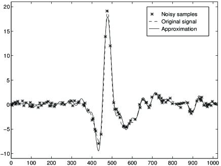
Figure 6.2: Approximation using Algorithm 3.1, terminated at level 19.

Recall that we have had to use a different stopping criterion than for Algorithm 3.1 to prove convergence of the CG–multi-level algorithm. The CG-stopping criterion (2.10) forces the algorithm to terminate earlier, thus giving a weaker approximation, see Figure 6.3. Although we cannot justify it theoretically, we always got very good reconstructions in our numerical experiments by using the same stopping criterion as for the Landweber-Richardson multi-level algorithm, compare Figure 6.4.

Figure 6.3: Approximation using Algorithm 2.3, terminating at level 13.

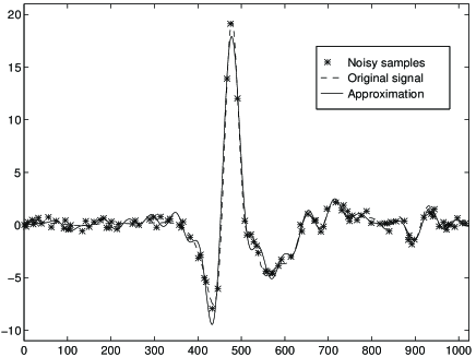
Figure 6.4: Approximation using Algorithm 2.3, using stopping criterion 3.1, terminating at level 19.

Note that our numerical experiments indicate that for most practical applications one can drop the factor 2 in the discrepancy principle (3.19). In this case Algorithm 3.1 terminates at level 23 and the approximation error is $0.09$, see also Figure 6.5.

Figure 6.5: Approximation using Algorithm 3.1, omitting the factor 2 in the stopping criterion 3.1, terminating at level 23.

Experiment 2: We use the same signal and the same noise level as in Experiment 1, but only 89 sampling points that are in addition more irregularly distributed with a standard deviation $\sigma=12.2$. Thus the operators $T_{N}$ have a larger condition number than those arising in Experiment 1. This experiment demonstrates that a proper choice of the bandwidth can serve as a regularization procedure. Algorithm 3.1 terminates at level $N_{*}=18$, the final error between the original signal and the approximation is 0.19. The reconstruction is shown in Figure 6.6. It is remarkable that this approximation is better than the approximation we obtain when we apply the standard CGNE method 2 directly using the a priori information about the “correct level” $M=30$. In this case the approximation error is 0.28, thus substantially larger. The approximation is shown in Figure 6.7.

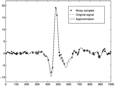
Figure 6.6: Approximation using Algorithm 3.1 providing an approximation error $\|x_{*}-x^{\delta}_{k_{*},N_{*}}\|/\|x\|=0.19$.

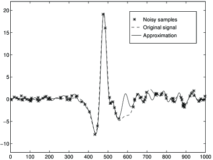
Figure 6.7: Approximation using standard CGNE directly for level $M=30$, providing an approximation error $\|x_{*}-x^{\delta}_{N}\|/\|x\|=0.28$.

Experiment 3: We consider the reconstruction of a signal representing a dynamical response of a mechanical system. The signal has been sampled at 300 irregularly spaced points with $\sigma=40.7$, the original signal itself is not known. We run Algorithm 3.1 without using any other a priori information about the signal than the samples and the measurement error which is known from experience to be approximately $10\%$.

Algorithm 3.1 terminates at level 42, the approximation is displayed in Figure 6.8 as solid line. In the chosen discrete model [FGS95], $N=42$ means that the reconstruction is a trigonometric polynomial of degree 42. Since the number of sampling values is 300, we have about 3.5 times as many samples as we would need theoretically to determine a reasonable approximation. Thus we should obtain about the same bandwidth and approximation by using only every second sampling value, since we still have enough samples and the corresponding operators $T_{N}$ are still well-conditioned. It turns out that the algorithm terminates again at level 42, giving an approximation close the first one. The normalized error between both approximations is $11\%$. Having in mind that we have used only $50\%$ of the given samples and that the measurement error is about $10\%$, this result demonstrates the robustness of the proposed algorithms. The approximation for using only half of the samples is displayed in Figure 6.8 as dotted line.

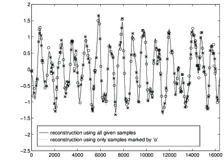
Figure 6.8: Two reconstructions of dynamical impulse response using Algorithm 3.1.

References

- [BG68] G. Backus and F. Gilbert. The resolving power of gross earth data. Geophys. J. R. Astr. Soc., 16: 169–205, 1968.
- [Ben92] J. Benedetto. Irregular sampling and frames. In C. K. Chui, editor, Wavelets: A Tutorial in Theory and Applications, pages 445–507. Academic Press, 1992.
- [BL97] J. Benedetto and S. Li. The theory of multiresolution analysis frames and applications to filter banks. Appl. Comp. Harm. Anal., to appear.
- [Chr96] O. Christensen. Moment problems and stability results for frames with applications to irregular sampling and Gabor frames. J. Appl. Comp. Harm. Anal., 3/1: 82–86, 1996.
- [Dau92] I. Daubechies. Ten Lectures on Wavelets. CBMS-NSF Reg. Conf. Series in Applied Math. SIAM, 1992.
- [FG94] H.G. Feichtinger and K.H. Gröchenig. Theory and practice of irregular sampling. In J. Benedetto and M. Frazier, editors, Wavelets: Mathematics and Applications, pages 305–363. CRC Press, 1994.
- [FGS95] H. G. Feichtinger, K. Gröchenig, and T. Strohmer. Efficient numerical methods in non-uniform sampling theory. Numerische Mathematik, 69:423–440, 1995.
- [Gro93] K. Gröchenig. A discrete theory of irregular sampling. Lin. Alg. and Appl., 193:129–150, 1993.
- [Gro84] C.W. Groetsch. The Theory of Tikhonov Regularization for Fredholm Integral Equations of the First Kind. Pitman, Boston, 1984.
- [HNS95] M. Hanke, A. Neubauer and O. Scherzer. A convergence analysis of the Landweber iteration for nonlinear ill–posed problems. Numerische Mathematik, 71: 21–37, 1995.
- [Han96] M. Hanke. Regularizing properties of a truncated Newton–CG Algorithm for nonlinear inverse problems. Preprint Nr. 280, Universität Kaiserslautern, Germany, 1996.
- [EHN96] H.W. Engl, M. Hanke and A. Neubauer. Regularization of Inverse Problems. Kluwer Academic Publishers, Dortrecht, 1996.
- [Han95] M. Hanke. Conjugate Gradient Type Methods for Ill–Posed Problems. Longman Scientific and Technical, Harlow, Essex, 1995.
- [Hig96] J.R. Higgins. Sampling Theory in Fourier and Signal Analysis: Foundations. Oxford University Press, 1996.
- [Ist87] V.I. Istratescu. Inner Product Structures. Mathematics and its Applications. D. Reidel, Dordrecht, Holland, 1987.
- [LM91] A.K. Louis and P. Maaß. Smoothed projection methods for the moment problem. Numerische Mathematik, 59:277–294, 1991.
- [Mal89] S. Mallat. Multiresolution Approximation and Wavelets. Trans. of American Math. Soc., 315:69–88, 1989.
- [NW91] M.Z. Nashed and G.G. Walter. Generalized sampling theorems for functions in reproducing kernel Hilbert spaces. Math. of Control, Signals and Systems, 4:363–390, 1991.
- [RSar] M. Rauth and T. Strohmer. Smooth approximation of potential fields from noisy scattered data. Geophysics, to appear.
- [Sai88] S. Saitho. Theory of Reproducing Kernels and Its Applications. Longman Scientific and Technical, 1988.
- [Sam95] Proc. of SampTA’95 – Workshop on Sampling Theory & Applications Jurmala, Latvia. September 1995.
- [Sch96] O. Scherzer. A multi–level algorithm for the solution of nonlinear ill–posed problems. Numer. Math., to appear.
- [You80] R. Young. An Introduction to Nonharmonic Fourier Series. Academic Press, New York, 1980.
- [XN94] X.-G. Xia and M. Z. Nashed. The Backus–Gilbert method for signals in reproducing kernel Hilbert spaces and wavelet subspaces. Inverse Problems, 10: 785–804, 1994.
- [Zay93] A.I. Zayed. Advances in Shannon’s Sampling Theory. CRC Press, Boca Raton, 1993.