Extremal Approximately Convex Functions and Estimating the Size of Convex Hulls

Abstract.

A real valued function $f$ defined on a convex $K$ is an approximately convex function iff it satisfies

$$f\Bigl{(}\frac{x+y}{2}\Bigr{)}\leq\frac{f(x)+f(y)}{2}+1.$$

A thorough study of approximately convex functions is made. The principal results are a sharp universal upper bound for lower semi-continuous approximately convex functions that vanish on the vertices of a simplex and an explicit description of the unique largest bounded approximately convex function $E$ vanishing on the vertices of a simplex.

A set $A$ in a normed space is an approximately convex set iff for all $a,b\in A$ the distance of the midpoint $(a+b)/2$ to $A$ is $\leq 1$. The bounds on approximately convex functions are used to show that in ${\mathbf{R}}^{n}$ with the Euclidean norm, for any approximately convex set $A$, any point $z$ of the convex hull of $A$ is at a distance of at most $[\log_{2}(n-1)]+1+(n-1)/2^{[\log_{2}(n-1)]}$ from $A$. Examples are given to show this is the sharp bound. Bounds for general norms on ${\mathbf{R}}^{n}$ are also given.

1. Introduction

The problem motivating this paper is the following: given a set $A$ in ${\mathbf{R}}^{n}$, estimate the size of the convex hull $\operatorname{Co}\nolimits(A)$ of $A$ in terms of geometric properties of $A$. To do this we assume that ${\mathbf{R}}^{n}$ is equipped with a norm $\|\cdot\|$. Then a first step in constructing the convex hull of $A$ is to add all the midpoints of segments joining points of $A$. The size of $\operatorname{Co}\nolimits(A)$ can be estimated in terms of this first step.

Our main result gives the sharp constants in this estimate for $n$-dimensional Euclidean spaces and it provides an estimate for the constants for general $n$-dimensional normed spaces which is accurate to within $2/n$. (Here $\operatorname{dist}\nolimits(x,A):=\inf\{\|x-a\|:a\in A\}$ is the distance of the point $x$ from the set $A$.)

Theorem 1.

If $({\mathbf{R}}^{n},\|\cdot\|)$ is an $n$-dimensional normed linear space then there is a constant $C_{\|\cdot\|}$, depending on the norm $\|\cdot\|$, so that if $A\subset{\mathbf{R}}^{n}$ satisfies

(1.1) $$a_{0},a_{1}\in A\quad\text{implies}\quad\operatorname{dist}\nolimits\Big{(}\frac{a_{0}+a_{1}}{2},A\Big{)}\leq\delta,$$

then

$$z\in\operatorname{Co}\nolimits(A)\quad\text{implies}\quad\operatorname{dist}\nolimits(z,A)\leq C_{\|\cdot\|}\delta.$$

Letting $[\,\cdot\,]$ be the greatest integer function, the sharp constant $C_{\|\cdot\|}$ satisfies

$$[\log_{2}(n-1)]+1+(n-1)/2^{[\log_{2}(n-1)]}\leq C_{\|\cdot\|}\leq[\log_{2}(n)]+1+n/2^{[\log_{2}(n)]}$$

(this holds for all norms) and the sharp constant when $\|\cdot\|$ is the Euclidean norm is $C_{\|\cdot\|}=[\log_{2}(n-1)]+1+(n-1)/2^{[\log_{2}(n-1)]}$.

The upper bound $C_{\|\cdot\|}\leq 2\lceil\log_{2}(n+1)\rceil$ (where $\lceil\cdot\rceil$ is the ceiling function) is implicit in the paper [1, Props 3.3 and 3.4] of Casini and Papini.

For bounded sets this can be given a concise restatement in terms of the Hausdorff distance between sets. Recall that if $A,B\subset{\mathbf{R}}^{n}$ are bounded then the Hausdorff distance, $d_{H}(A,B)$, between $A$ and $B$ is the infimum of the numbers $r$ so that every point of $A$ is within a distance $r$ of a point of $B$ and every point of $B$ is within distance $r$ of a point of $A$. Define numbers $\kappa(n)$ for $n\geq 0$ by $\kappa(0):=0$ and

$$\kappa(n):=[\log_{2}(n)]+1+n/2^{[\log_{2}(n)]}$$

for $n\geq 1$. The collection of midpoints of segments joining pairs of points of $A$ is $\frac{1}{2}(A+A)=\{(a+b)/2:a,b\in A\}$. Then Theorem 1 can be restated as

$$d_{H}(\operatorname{Co}\nolimits(A),A)\leq C_{\|\cdot\|}d_{H}\Big{(}\frac{1}{2}(A+A),A\Big{)}$$

where the sharp constant $C_{\|\cdot\|}$ satisfies

$$\kappa(n-1)\leq C_{\|\cdot\|}\leq\kappa(n)$$

and $C_{\|\cdot\|}=\kappa(n-1)$ when $\|\cdot\|$ is the Euclidean norm. (Allowing $+\infty$ for a value of $d_{H}(A,B)$ this also holds for unbounded sets). If $A$ is a finite set with $N$ points, then $d_{H}(A,\frac{1}{2}(A+A))=\max_{b,c\in A}\min_{a\in A}\|a-\frac{1}{2}(b+c)\|$ which can be computed in $O(N^{3})$ operations. Thus for finite sets Theorem 1 allows estimation of $d_{H}(A,\operatorname{Co}\nolimits(A))$ in polynomial time.

For general norms obtaining the lower bound $\kappa(n-1)\leq C_{\|\cdot\|}$ is more difficult than the upper bound and involves construction of some interesting geometric objects, the extremal approximately convex functions. To describe these we first make a couple of definitions. The following is motivated by taking $\delta=1$ in the hypothesis of Theorem 1.

Definition 1.

Let $({\mathbf{X}},\|\cdot\|)$ be a normed space. Then a subset $A\subset{\mathbf{X}}$ is an approximately convex set iff for all $a,b\in A$

$$\operatorname{dist}\nolimits\Bigl{(}\frac{1}{2}(a+b),A\Bigr{)}\leq 1.$$

∎

If $A$ is an approximately convex set then the function $h(x)=\operatorname{dist}\nolimits(x,A)$ (the distance of $x$ from $A$) will satisfy a weak form of the inequality satisfied by a convex function. We isolate this property:

Definition 2.

Let $E$ be a convex set in the normed space $({\mathbf{X}},\|\cdot\|)$. Then a function $h\colon E\to{\mathbf{R}}$ is an approximately convex function iff for all $a,b\in E$

$$h\Bigl{(}\frac{a+b}{2}\Bigr{)}\leq\frac{h(a)+h(b)}{2}+1.$$

∎

(Strictly speaking this should be “approximately midpoint convex” or “approximately Jensen convex” but for the sake of brevity we will use “approximately convex”.) Let $\Delta_{n}:=\{(\alpha_{0},\dots,\alpha_{n}):\alpha_{k}\geq 0,\ \sum_{k=0}^{n}\alpha_{k}\}$ be the standard $n$-dimensional simplex. Then the result leading to the lower bounds on $C_{\|\cdot\|}$ is the explicit computation of the extremal approximately convex function on the simplex.

Theorem 2.

There is an approximately convex $E\colon\Delta_{n}\to{\mathbf{R}}$ which vanishes on the vertices of $\Delta_{n}$ with the following properties:

1. If $h$ is a bounded (or Borel-measurable) approximately convex function on $\Delta_{n}$ which takes non-positive values on the vertices, then $h(x)\leq E(x)$ for $x\in\Delta_{n}$.

2. $E$ achieves its maximum value of $\kappa(n)$.

3. $E$ is lower semi-continuous.

The property 1 characterizes $E$ uniquely. Moreover $E$ is given concretely in terms of an elementary infinite sum (see equations (2.19) and (2.21)).

The examples showing the lower bounds on $C_{\|\cdot\|}$ in Theorem 1 are sharp and are constructed from the graph of $E$. The lower semi-continuity of $E$ and the fact that $E$ has $\kappa(n)$ as its maximum are important in these constructions. We note the mere existence of $E$ (which follows from abstract considerations) is less important than the fact that $E$ is given explicitly in a relatively simple form (cf. §2.4 and Figure 2).

We now give a more detailed description of our results. In §2.1 we give upper bounds on approximately convex functions which are locally bounded from above. Motivated by Perron’s method in the theory of harmonic functions in §2.2 we show that given a compact convex set $K\subset{\mathbf{R}}^{n}$ with extreme points $V$ and a uniformly continuous function $\varphi\colon V\to{\mathbf{R}}$ then there is a a unique extremal bounded approximately convex function $E_{K,\varphi}$ on $K$ which agrees with $\varphi$ on $V$; moreover, $E_{K,\varphi}$ is realized (as in Perron’s method) as the pointwise supremum of all bounded approximately convex functions on $K$ which agree with $\varphi$ on $V$. The function $E_{K,\varphi}$ is lower semi-continuous, characterized by a mean-value property, and satisfies a certain maximum principle.

§2.3 and §2.4 contain a description of the extremal approximately convex function $E$ on the simplex and proofs of the properties of $E$ listed in Theorem 2. In § 2.5, we determine the extremal function $E_{K,\varphi}$ when $K$ is a convex polytope. A stability theorem with sharp constants for approximately convex functions of the type first given by Hyers and Ulam [4] is given in §2.6. This states that an approximately convex function can be approximated in the uniform norm by a convex function with error only depending on the dimension of the domain. The example showing the constants are sharp is the extremal function $E$. The rest of Section 2 gives various other properties and examples of approximately convex functions.

Section 3 gives the proof of Theorem 1 and some of its extensions and refinements. The first two sections give the upper and lower bounds $\kappa(n-1)\leq C_{\|\cdot\|}\leq\kappa(n)$ for general norms. The upper bound follows from the general upper bounds on approximately convex functions and the lower bound uses properties of the extremal approximately convex function $E$ on $\Delta_{n}$. The proof that $C_{\|\cdot\|}=\kappa(n-1)$ in the Euclidean case is given in §3.3. This requires some (hopefully interesting) geometrical arguments in addition to Theorem 2. Finally, we prove that $C_{\|\cdot\|}=2$ for all two-dimensional norms. This argument is somewhat ad hoc and does not appear to extend to higher dimensions.

2. Approximately Convex Functions

We first relate approximately convex functions to approximately convex sets.

2.1 Proposition.

Let $({\mathbf{X}},\|\cdot\|)$ be a normed space, $A\subset{\mathbf{X}}$, and define $h(x):=\operatorname{dist}\nolimits(x,A)$. Then $A$ is an approximately convex set if and only if $h$ is an approximately convex function.

Proof.

If $h(x)=\operatorname{dist}\nolimits(x,A)$ is an approximately convex function it is clear that $A$ is an approximately convex set. Conversely if $A$ is an approximately convex set, let $x_{0},x_{1}\in{\mathbf{X}}$ and $\varepsilon>0$. Choose $a_{0},a_{1}\in A$ so that $h(x_{0})=\operatorname{dist}\nolimits(x_{0},A)\leq\|x_{0}-a_{0}\|+\varepsilon$ and $h(x_{1})\leq\|x_{1}-a_{1}\|+\varepsilon$. As $A$ is approximately convex $\operatorname{dist}\nolimits((a_{0}+a_{1})/2,A)\leq 1$. Thus

$$\operatorname{dist}\nolimits\Bigl{(}\frac{x_{0}+x_{1}}{2},A\Bigr{)} \leq\Bigl{\|}\frac{x_{0}-a_{0}}{2}\Bigr{\|}+\Bigl{\|}\frac{x_{1}-a_{1}}{2}\Bigr{\|}+\operatorname{dist}\nolimits(\frac{a_{0}+a_{1}}{2},A)$$

$$\leq\frac{h(x_{0})+h(x_{1})}{2}+\varepsilon+1$$

As $\varepsilon$ as arbitrary this completes the proof. (This proof is implicit in the paper of Casini and Papini [1, Prop. 3.4].) ∎

2.1. Bounds on approximately convex functions

The first bound is an extension to approximately convex functions of a standard result about convex functions.

2.2 Proposition.

Let $U\subseteq{\mathbf{R}}^{n}$ be a convex set and $h\colon U\to{\mathbf{R}}$ be approximately convex and bounded from above by $C$. Then for any $x_{0}\in U$ and $x\in U\cap(2x_{0}-U)$ (if $x_{0}$ is in the interior of $U$ this is a neighborhood of $x_{0}$ in $U$) the inequality

$$h(x)\geq 2h(x_{0})-C-2$$

holds, and so $h$ is bounded from below in $U\cap(2x_{0}-U)$. Thus $h$ is bounded from below on compact subsets of the interior of $U$.

Proof.

Let $y=2x_{0}-x$. Then $y\in U$ as $x\in(2x_{0}-U)$. Also $x_{0}=(x+y)/2$. Thus

$$h(x_{0})=h\Bigl{(}\frac{x+y}{2}\Bigr{)}\leq\frac{h(x)+h(y)}{2}+1\leq\frac{h(x)+C}{2}+1.$$

Solving this for $h(x)$ completes the proof. ∎

The following theorem is one of our main results.

2.3 Theorem.

Let $A\subset{\mathbf{R}}^{n}$ with convex hull $E=\operatorname{Co}\nolimits(A)$. Let $h\colon E\to{\mathbf{R}}$ be an approximately convex function which is bounded above and which satisfies $h\leq 0$ on $A$. Then

$$\sup_{x\in E}h(x)\leq[\log_{2}n]+1+\dfrac{n}{2^{[\log_{2}n]}}.$$

Moreover this is the sharp upper bound (the sharpness follows from Theorem 2.27).

2.4 Remark.

The assumption that $h$ is bounded above can not be dropped. For the relevant example see Example 2.42 in §2.7 below.∎

Before giving the proof we give a name to the bounds in the Theorem and show that they satisfy a recursion which is a main ingredient of the proof. Let $\kappa(0)=0$ and for $n\geq 1$

(2.1) $$\kappa(n)=[\log_{2}n]+1+\dfrac{n}{2^{[\log_{2}n]}}.$$

This notation will be use throughout the rest of the paper.

2.5 Proposition.

The sequence $\langle\kappa(n)\rangle_{k=0}^{\infty}$ satisfies the recursion

(2.2) $$\kappa(n)=\max_{\begin{subarray}{c}n_{1}+n_{2}=n\\ \vphantom{I}n_{1},n_{2}\geq 0\end{subarray}}\frac{\kappa(n_{1})+\kappa(n_{2})}{2}+1$$

for $n\geq 1$.

2.6 Lemma.

Let $\langle\alpha(i)\rangle_{i=0}^{m}$ be a finite sequence on $\{0,1,\dots,m\}$ so that $\langle\alpha(j)-\alpha(j-1)\rangle_{j=1}^{m}$ is monotone decreasing (that is the sequence is concave). Then

$$\max_{i+j=n}\frac{\alpha(i)+\alpha(j)}{2}+1=\begin{cases}\alpha(n)+1=\dfrac{\alpha(n)+\alpha(n)}{2}+1,&m=2n;\\ \dfrac{\alpha(n)+\alpha(n+1)}{2}+1,&m=2n+1.\end{cases}$$

Proof.

Let $\beta(i)=(\alpha(i)+\alpha(n-i))/{2}+1$. Then the concavity of $\langle\alpha(i)\rangle$ implies the sequence $\langle\beta(i)\rangle$ is also concave. Also $\beta(i)=\beta(n-i)$ so $\langle\beta(i)\rangle$ is symmetric. But a symmetric concave function takes on its maximum at the center of its interval of definition. Thus if $m=2n$ is even the maximum is $\beta(n)=\alpha(n)+1$ and if $m=2n+1$ the maximum is $\beta(n)=\beta(n+1)=(\alpha(n)+\alpha(n+1))/2+1$. ∎

Proof of Proposition 2.5.

A calculation shows

$$\kappa(2n)=\kappa(n)+1,\quad\kappa(2n+1)=\frac{\kappa(n)+\kappa(n+1)}{2}+1.$$

(The second of these is most easily seen by writing $n=2^{m}+r$ where $0\leq r\leq 2^{m}-1$.) But the sequence $\langle\kappa(n)-\kappa(n-1)\rangle_{k=1}^{\infty}$ is monotone decreasing so that an application of the last lemma completes the proof. ∎

Proof of Theorem 2.3.

Recalling the definition of $\kappa(n)$ we wish to show that $\sup_{x\in E}h(x)\leq\kappa(n)$ We use induction on $n$ based on the recursion (2.2) satisfied by $\kappa$. The base case of $n=0$ is clear. Suppose $n\geq 1$ and assume that the assertion holds for all integers less than $n$. If $x\in E$ then by Carathéodory’s Theorem (cf. [7, p. 3]) there are $x_{0},\dots,x_{n}\in A$ so that $x\in\operatorname{Co}\nolimits\{x_{0},\dots,x_{n}\}$. Thus without loss of generality we may assume that $E=\operatorname{Co}\nolimits\{x_{0},\dots,x_{n}\}$. Let $M:=\sup_{x\in E}h(x)<\infty$ and let $\varepsilon>0$. Suppose that $x=\sum_{k=0}^{n}\alpha_{k}x_{k}\in E$ (with $\sum_{k=0}^{n}\alpha_{k}=1$ and $\alpha_{k}\geq 0$) and $h(x)\geq M-\varepsilon$. By reordering the terms if necessary we may assume $\alpha_{0}\leq\alpha_{1}\leq\dots\leq\alpha_{n}$. Note that $\alpha_{0}\leq 1/(n+1)\leq 1/2$. Let $n_{1}$ be the least integer so that

$$\sum_{k=0}^{n_{1}}\alpha_{k}>\frac{1}{2}.$$

Then $\sum_{k=0}^{n_{1}-1}\alpha_{k}\leq\frac{1}{2}$. Set

$$s=\frac{1}{2}-\sum_{k=0}^{n_{1}-1}\alpha_{k},\quad t=\alpha_{n_{1}}-s,$$

and let

$$y=2\biggl{(}\sum_{k=0}^{n_{1}-1}x_{k}+sx_{n_{1}}\biggr{)},\quad z=2\biggl{(}tx_{n_{1}}+\sum_{n_{1}+1}^{n}\alpha_{k}x_{k}\biggr{)}.$$

Then $y\in E$ as $\sum_{k=0}^{n_{1}-1}\alpha_{k}+s=\frac{1}{2}$. Likewise $z\in E$. In particular $y\in\operatorname{Co}\nolimits\{x_{0},\dots,x_{n_{1}}\}=:\Delta_{1}$ and $z\in\operatorname{Co}\nolimits\{x_{n_{1}},\dots,x_{n}\}=:\Delta_{2}$. Then $\dim\Delta_{1}=n_{1}$ and $\dim\Delta_{2}=n-n_{1}=:n_{2}$. Since $\alpha_{0}\leq 1/2$ we have $n_{1}\geq 1$.

If $n_{1}<n$ then $n_{1},n_{2}<n$ and therefore by the induction hypothesis and $x=\frac{1}{2}(y+z)$, we have

$$M-\varepsilon \leq h(x)\leq\frac{h(y)+h(z)}{2}+1\leq\frac{\kappa(n_{1})+\kappa(n_{2})}{2}+1$$

$$\leq\kappa(n_{1}+n_{2})=\kappa(n).$$

Therefore $M\leq\kappa(n)+\varepsilon$. This leaves the case $n_{1}=n$. Then $z=x_{n}\in A$ and thus $h(z)=0$. Whence

$$M-\varepsilon\leq h(x)\leq\frac{h(y)+h(z)}{2}+1=\frac{h(y)}{2}+1\leq\frac{M}{2}+1.$$

Solve this inequality for $M$ and use $2\leq\kappa(n)$ to get $M\leq 2(1+\varepsilon)\leq\kappa(n)(1+\varepsilon)$. Combining the inequalities from the two cases and letting $\varepsilon\searrow 0$ implies $M\leq\kappa(n)$ and completes the proof. ∎

2.7 Remark.

As many of our results will involve $\kappa(n)$ it is worth giving some sharp bounds on $\kappa(n)$. To do this extend $\kappa$ to the positive reals by defining $\kappa(x)=[\log_{2}x]+1+x/{2^{[\log_{2}x]}}$. Then for any integer $m$ we have $\kappa(2^{m})=m+2=\log_{2}(2^{m})+2$. On closed intervals $[2^{m},2^{m+1}]$ the function $\kappa(x)$ is linear. Thus $\kappa(x)$ is the continuous piecewise linear function on $(0,\infty)$ with knots at $x=2^{m}$ and with $\kappa(x)=2+\log_{2}(x)$ at the knots. As the function $2+\log_{2}(x)$ is concave this implies $\kappa(x)\leq 2+\log_{2}(x)$. On each of the intervals it is a straightforward calculus exercise to find the maximum of $(2+\log_{2}(x))-\kappa(x)$ on the interval $[2^{m},2^{m+1}]$. The result is $(\ln(2)-\ln(\ln(2))-1)/\ln(2)\approx.08607133206$ (surprisingly this is independent of which interval $[2^{m},2^{m+1}]$ we are working on). This leads to the bounds

$$1.913928+\log_{2}(n)<\kappa(n)\leq 2+\log_{2}(n).$$

∎

2.2. Lower semi-continuity and mean value properties of extremal approximately convex functions

Let $K\subset{\mathbf{R}}^{n}$ be a compact convex set and let $V$ be the set of extreme points of $K$. Let $\varphi\colon V\to R$ be a function. Then a function $h\colon K\to{\mathbf{R}}^{n}$ has extreme values equal to $\varphi$ iff $h\big{|}_{V}=\varphi$. (The terminology is a variant on that used in partial differential equations where the boundary values of a function are often prescribed.) Likewise if $f,g\colon K\to{\mathbf{R}}$ are two functions then $f$ and $g$ have the same extreme values iff they agree on $V$. If $\varphi\colon V\to{\mathbf{R}}$, let ${\mathcal{B}}(K,\varphi)$ be the set of bounded approximately convex functions $h$ so that $h\big{|}_{V}\leq\varphi$ on $V$. Then the extremal approximately convex function with extreme values equal to $\varphi$ is

(2.3) $$E_{K,\varphi}(x)=\sup_{h\in{\mathcal{B}}(K,\varphi)}h(x).$$

This is the pointwise largest approximately convex function with extreme values $\leq\varphi$ on $V$. While in general we may have $E_{K,\varphi}(v)<\varphi(v)$ for some $v\in V$, we will show that if $\varphi$ is uniformly continuous on $V$ (which will always be the case if $V$ is finite) then $E_{K,\varphi}\big{|}_{V}=\varphi$ and that $E_{K,\varphi}$ is lower semi-continuous on $K$.

Let $K\subset{\mathbf{R}}^{n}$ be a compact set with extreme points $V$. Then for any function $h\colon K\to{\mathbf{R}}$ which is bounded above define $Sh$ by

$$Sh(x)=\begin{cases}h(x),&x\in V;\\ {\displaystyle\inf\Bigl{\{}\dfrac{h(y)+h(z)}{2}+1}\ :\ \dfrac{y+z}{2}=x\Bigr{\}},&x\in K\setminus V.\end{cases}$$

This operator is closely related to approximately convex functions as

(2.4) $$f\leq Sf\quad\iff\quad\text{$f$ is approximately convex on $K$.}$$

Despite being nonlinear $S$ is somewhat like a mean value operator. We make this more precise by proving a maximum principle for the equation $Sf=f$.

2.8 Theorem.

Let $K\subset{\mathbf{R}}^{n}$ be a compact convex set with extreme points $V$. Let $f,F\colon K\to{\mathbf{R}}$ be bounded functions so that $Sf\leq f$ and $F$ is approximately convex (that is $SF\geq F$). Let

(2.5) $$L(x)=\min\{f(x),\liminf_{y\to x}f(y)\}$$

be the lower semi-continuous envelope of $f$. Then

(2.6) $$\sup_{x\in K}(F(x)-f(x))=\sup_{v\in V}(F(v)-f(v))$$

and

(2.7) $$\sup_{x\in K}(F(x)-L(x))=\sup_{v\in V}(F(v)-L(v)).$$

Proof.

We will prove (2.7), the proof of (2.6) being similar (and a little easier). The inequality $Sf\leq f$ implies that if $x\notin V$ then

(2.8) $$f(x)\geq\inf\Bigl{\{}\frac{f(y)+f(z)}{2}+1\,:\,\frac{y+z}{2}=x\Bigl{\}}.$$

As $f$ and $F$ are bounded we may assume (after possibly adding positive constants to $f$ and $F$) that $0\leq f\leq F\leq M$ for some positive constant $M$. This implies $0\leq L\leq F$. Set $\omega(x):=F(x)-L(x)$ and $\delta:=\sup_{x\in K}\omega(x)$. Then we wish to show $\sup_{v\in V}\omega(v)=\delta$. If $\delta=0$ then $L\equiv F$ and there is nothing to prove. So assume $\delta>0$. Choose a positive integer $N$ so that $N>M$. Let $0<\varepsilon<1$ and choose $w_{0}$ to be a point so that $\omega(w_{0})>(1-\varepsilon 2^{-N})\delta$. Suppose that $w_{0}\notin V$ for sufficiently small $\varepsilon>0$ (otherwise the desired conclusion follows as $\varepsilon\to 0$). From the definition of $L$ there is a sequence $\langle x_{k}\rangle_{k=1}^{\infty}$ such that $x_{k}\to w_{0}$ and $f(x_{k})\to L(w_{0})$. By equation (2.8) there are sequences $\langle y_{k}\rangle_{k=1}^{\infty}$ and $\langle z_{k}\rangle_{k=1}^{\infty}$ such that $x_{k}=(y_{k}+z_{k})/2$ and a real number $C\geq 0$ such that

(2.9) $$f(x_{k})-\Bigl{(}\frac{f(y_{k})+f(z_{k})}{2}+1\Bigr{)}\to C\geq 0$$

By passing to a subsequence we may assume that $y_{k}\to y$, $z_{k}\to z$, $f(y_{k})\to A$, and $f(z_{k})\to B$ for some $y,z\in K$ and $A,B\in{\mathbf{R}}$. Clearly $w_{0}=(y+z)/2$ and (using the definition of $L$) $L(y)\leq A$, $L(z)\leq B$. Then (2.9) yields

(2.10) $$L(w_{0})=\frac{A+B}{2}+1+C\geq\frac{L(y)+L(z)}{2}+1$$

and so

(2.11) $$F(w_{0})=L(w_{0})+\omega(w_{0})\geq\frac{L(y)+L(z)}{2}+1+\omega(w_{0}).$$

But since $F$ is approximately convex

(2.12) $$F(w_{0})\leq\frac{F(y)+F(z)}{2}+1=\frac{L(y)+L(z)}{2}+1+\frac{\omega(y)+\omega(z)}{2}.$$

Combining (2.12) and (2.11) yields

(2.13) $$\frac{\omega(y)+\omega(z)}{2}\geq\omega(w_{0}).$$

Since $\delta=\sup_{x\in K}\omega(x)$ and $\omega(w_{0})\geq(1-\varepsilon 2^{-N})\delta$, (2.13) implies

$$\min\{\omega(y),\omega(z)\}\geq 2\omega(w_{0})-\delta\geq(2(1-\varepsilon 2^{-N})-1)\delta=(1-\varepsilon 2^{-(N-1)})\delta.$$

From (2.10) have $\min\{L(y),L(z)\}\leq L(w_{0})-1$. Without loss of generality we may assume that $L(y)\leq L(w_{0})-1$. Let $w_{1}=y$. Then $L(w_{1})\leq L(w_{0})-1$ and $\omega(w_{1})\geq(1-\varepsilon 2^{-(N-1)})$.

If $w_{1}\notin V$ then we can repeat this argument (with $N$ replaced by $N-1$) and get a $w_{2}\in K$ with $L(w_{2})\leq L(w_{1})-1$ and $\omega(w_{1})\geq(1-\varepsilon 2^{N-2})\delta$. We continue in this manner to get a finite sequence $w_{0},w_{1},\dots,w_{m}$ with $m<N$ so that for $1\leq k\leq m-1$ we have $L(w_{k})\leq L(w_{k-1})-1$, $\omega(w_{k})\geq(1-\varepsilon 2^{N-k})\delta$, and $w_{k}\notin V$. (Note this can not continue for $k\geq N$ as that would imply $L(w_{N})\leq L(w_{0})-N\leq M-N<0$ contradicting $L\geq 0$. Thus $w_{m}\in V$ for some $m<N$.) At the last step $w_{m}\in V$ and $\omega(w_{m})\geq(1-\varepsilon 2^{-(N-m)})\delta$. Therefore $\sup_{v\in V}\omega(v)\geq(1-\varepsilon 2^{-(N-m)})\delta$. Letting $\varepsilon\searrow 0$ yields $\sup_{v\in V}\omega(v)\geq\delta$. But $\sup_{v\in V}\omega(v)\leq\delta$ is clear. Thus $\sup_{v\in V}\omega(v)=\delta$ as required. ∎

2.9 Proposition.

Let $K\subset{\mathbf{R}}^{n}$ be a compact convex set with extreme points $V$ and let $h\colon K\to{\mathbf{R}}^{n}$ be a bounded approximately convex function on $K$. Then $h(x)\leq Sh(x)$, the functions $h$ and $Sh$ have the same extreme values, $Sh$ is approximately convex, and if $h$ is lower semi-continuous as a function on $K$ at points of $V$ then the same is true of $Sh$.

Proof.

If $x=(y+z)/2$ then as $h$ is approximately convex $h(x)\leq(h(y)+h(z))/2+1$ and taking the infimum yields $h(x)\leq Sh(x)$. That $h$ and $Sh$ have the same extreme values is clear. Using the definition of $Sh$ and the inequality $h\leq Sh$ we have

$$Sh\Bigl{(}\frac{y+z}{2}\Bigr{)}\leq\frac{h(y)+h(z)}{2}+1\leq\frac{Sh(y)+Sh(z)}{2}+1,$$

which shows $Sh$ is approximately convex. Finally if $h$ is lower semi-continuous at points of $V$ then for $x\in V$ we have $\liminf_{y\to x}Sh(y)\geq\liminf_{y\to x}h(y)\geq h(x)=Sh(x)$. This shows $Sh$ is lower semi-continuous at $x$ and completes the proof. ∎

We now characterize the extremal functions $E_{K,\varphi}$ as the unique bounded solutions to the equation $Sf=f$ with extreme values $\varphi$.

2.10 Theorem.

Let $K$ be a convex set with extreme points $V$ and $f\colon K\to{\mathbf{R}}$ a bounded function so that $Sf=f$. Let $\varphi:=f\big{|}_{V}$ be the extreme values of $f$ and let $E_{K,\varphi}$ be the extremal approximately convex function with extreme values $\varphi$. Then $f=E_{K,\varphi}$.

Proof.

The equality $Sf=f$ implies $f$ is approximately convex (cf. (2.4)). Then the extremal property of $E_{K,\varphi}$ implies $f\leq E_{K,\varphi}$. Let $F=E_{K,\varphi}$ in Theorem 2.8 and using that $f$ and $E_{K,\varphi}$ agree on $V$ we can use equation (2.6) to conclude $f=E_{K,\varphi}$. ∎

The following is an elementary variant on Corollary 17.2.1 in [6]. We include a short proof for completeness.

2.11 Proposition.

Assume $K\subset{\mathbf{R}}^{n}$ is a compact convex set and $V$ the set of extreme points of $K$. Let $\varphi\colon V\to{\mathbf{R}}$ be uniformly continuous. Then there exists a lower semi-continuous convex function $h\colon K\to{\mathbf{R}}$ so that $h\big{|}_{V}=\varphi$. Moreover we can choose $h$ so that $\inf_{x\in K}h(x)=\inf_{v\in V}\varphi(v)$ and $\sup_{x\in K}h(x)=\sup_{v\in V}\varphi(v)$.

Proof.

Let $\overline{V}$ be the closure of $V$. As $\varphi\colon V\to{\mathbf{R}}$ is uniformly continuous it has a unique continuous extension $\overline{\varphi}\colon\overline{V}\to{\mathbf{R}}$. Let Let $G_{\overline{\varphi}}:=\{(x,\overline{\varphi}(x)):x\in\overline{V}\}\subset K\times{\mathbf{R}}$ be the graph of $\overline{\varphi}$. As the set $\overline{V}$ is a compact and $\overline{\varphi}$ is continuous the set $G_{\overline{\varphi}}$ is also compact. Therefore the convex hull $\operatorname{Co}\nolimits(G_{\overline{\varphi}})$ is compact. Let $A:=\inf_{v\in V}\varphi(v)=\min_{x\in\overline{V}}\overline{\varphi}(x)$ and $B:=\sup_{v\in V}\varphi(v)=\max_{x\in\overline{V}}\overline{\varphi}(x)$. Then $\operatorname{Co}\nolimits(G_{\overline{\varphi}})\subseteq K\times[A,B]$. Moreover, as $K$ is the convex hull of its set of extreme points $V$, if $x\in K$ then there is $y\in[A,B]$ so that $(x,y)\in\operatorname{Co}\nolimits(G_{\varphi})$. Define $h$ by

$$h(x):=\min\{y:(x,y)\in\operatorname{Co}\nolimits(G_{\overline{\varphi}})\}.$$

It is clear from this definition that $h$ is convex and has the same supremum and infimum as $\varphi$. We now show that $h$ is lower semi-continuous. Let $a\in K$ and let $A:=\liminf_{x\to a}f(x)$. Choose a sequence $\langle x_{\ell}\rangle_{\ell=1}^{\infty}$ so that $x_{\ell}\to a$ and $h(x_{\ell})\to A$. Then as $\operatorname{Co}\nolimits(G_{\overline{\varphi}})$ is compact (and thus closed) the limit $\lim_{\ell\to\infty}(x_{\ell},h(x_{\ell}))=(a,A)\in\operatorname{Co}\nolimits(G_{\overline{\varphi}})$. The definition of $h$ then implies $h(a)\leq A=\liminf_{x\to a}h(x)$. Thus $h$ is lower semi-continuous at $a$ for every $a\in A$.

Finally let $v\in V$. Then as $(v,h(v))\in\operatorname{Co}\nolimits(G_{\overline{\varphi}})$ there exists $(\alpha_{0},\dots,\alpha_{n+1})\in\Delta_{n+1}$ and $v_{0},\dots,v_{n+1}\in\overline{V}$ so that $(v,h(v))=\sum_{k=0}^{n}\alpha_{k}(v_{k},\overline{\varphi}(v_{k}))$. But $v$ is an extreme point of $K$, which implies that $v_{k}=v$ for all $k$ and therefore $h(v)=\overline{\varphi}(v)=\varphi(v)$. ∎

2.12 Theorem.

Let $K\subseteq{\mathbf{R}}^{n}$ be a compact convex set with extreme points $V$. Assume that $\varphi\colon V\to{\mathbf{R}}$ is uniformly continuous. Then the extremal approximately convex function $E_{K,\varphi}$ satisfies $E_{K,\varphi}\big{|}_{V}=\varphi$ and is lower semi-continuous on $K$.

Proof.

By Proposition 2.11 there exists a lower semi-continuous convex function $h\colon K\to{\mathbf{R}}$ with extreme values $\varphi$. As $h$ is convex it is a fortiori approximately convex. $h$ approximately convex (so that $h\leq E_{K,\varphi}$) we have for $v\in V$ that $\varphi(v)=h(v)\leq E_{K,\varphi}(v)\leq\varphi(v)$, and so $E_{K,\varphi}$ has $\varphi$ as extreme values. As $h\leq E_{K,\varphi}$ and $h$ is lower semi-continuous, the function $E_{K,\varphi}$ will be lower semi-continuous at all points $x$ where $E_{K,\varphi}(x)=h(x)$. In particular, $E_{K,\varphi}$ will be lower semi-continuous at all points of $V$. Finally as $SE_{K,\varphi}\geq E_{K,\varphi}$ (cf. 2.9) the extremal property of $E_{K,\varphi}$ implies $SE_{K,\varphi}=E_{K,\varphi}$. Now in Theorem 2.8 let $f=F=E_{K,\varphi}$ and let $L$ be the lower semi-continuous envelope of $f=E_{K,\varphi}$ as given by (2.5). Then as $E_{K,\varphi}$ is lower semi-continuous at points of $V$ we have that $E_{K,\varphi}(v)=L(v)$ for all $v\in V$. Therefore (2.7) implies that $E_{K,\varphi}=L$ on $K$, so that $E_{K,\varphi}$ is lower semi-continuous as claimed. ∎

2.13 Remark.

Let $K\subset{\mathbf{R}}^{n}$ be a convex set with extreme points $V$. Let $h\colon K\to{\mathbf{R}}$ be a bounded approximately convex function and let $\varphi\colon V\to{\mathbf{R}}$ be the extreme values of $h$, that is $\varphi:=h\big{|}_{V}$. Then there is a bounded function $f\colon K\to{\mathbf{R}}$ such that $f\big{|}_{V}=\varphi$ for which the inequality $Sf\leq f$ holds pointwise on $K$. (Such a function exists as is seen by letting $f=E_{K,\varphi}$. On the simplex $\Delta_{n}$ with $\varphi=0$ the function $f(x)=k$ for $x$ in the interior of a $k$-dimensional face is an example of such a function.) Then define two sequences $\langle h_{k}\rangle_{k=0}^{\infty}$ and $\langle f_{k}\rangle_{k=0}^{\infty}$ of functions on $K$ by

$$h_{0}=h,\ h_{k+1}=Sh_{k},\quad f_{0}=f,\ f_{k+1}=Sf_{k}.$$

Then it can be shown that $f_{k+1}\leq f_{k}$, $h_{k+1}\geq h_{k}$, and that each $h_{k}$ is approximately convex. (The statements about $h_{k}$ follow from Proposition 2.9.) Also all the $h_{k}$’s and $f_{k}$’s have $\varphi$ as extreme values. Therefore both sequences have pointwise limits $h_{\infty}=\lim_{k\to\infty}h_{k}$ and $f_{\infty}=\lim_{k\to\infty}f_{k}$. These both have $\varphi$ as extreme values, $Sh_{\infty}=h_{\infty}$, and $Sf_{\infty}=f_{\infty}$. Therefore by Theorem 2.10 we have $h_{\infty}=f_{\infty}=E_{K,\varphi}$. This gives a method for finding $E_{K,\varphi}$ as the limit of two more or less constructively defined sequences. Also note that for each $k$ we have the inequalities

$$h_{k}\leq E_{K,\varphi}\leq f_{k}.$$

Thus we have explicit upper and lower bounds for $E_{K,\varphi}$.∎

2.3. The extremal approximately sub-affine function $H(x)$

A function $f\colon[0,1]\to{\mathbf{R}}$ is approximately sub-affine iff

(2.14) $$f\Bigl{(}\frac{x+y}{2}\Bigr{)}\leq\frac{f(x)+f(y)}{2}+\frac{x+y}{2}.$$

As in example 2.40 below approximately sub-affine functions can be used to construct approximately convex functions on a simplex. As a first step in explicitly describing the extremal approximately convex function on a simplex we describe the extremal approximately convex function on the unit interval.

Let ${\mathbf{N}}=\{0,1,2,\dots\}$ be the natural numbers and let ${\mathcal{D}}$ be the dyadic rational numbers in $[0,1]$. That is

$${\mathcal{D}}:=\Bigr{\{}\frac{m}{2^{n}}:m,n\in{\mathbf{N}}\text{ and }0\leq m\leq 2^{n}\Bigl{\}}.$$

(These play a considerable rôle in what follows.) The numbers in $[0,1]\setminus{\mathcal{D}}$ will be called the dyadic irrationals. Every dyadic irrational $x$ has a unique binary expansion $x=\sum_{i=0}^{\infty}{x_{i}}/{2^{i}}$ with $x_{i}\in\{0,1\}$. If $x\in{\mathcal{D}}$ then there are two binary expansions: the finite expansion $x=\sum_{i=0}^{N}{x_{i}}/{2^{i}}$ and, if $x_{N}=1$, there is also the infinite expansion $x=\sum_{i=0}^{N-1}{x_{i}}/{2^{i}}+\sum_{i=N+1}^{\infty}{1}/{2^{i}}$. Unless stated otherwise we will always use the finite expansion for an element of ${\mathcal{D}}$, even when we write $x=\sum_{i=0}^{\infty}x_{i}/2^{i}$ for notational uniformity. With this understood, define $H\colon[0,1]\to{\mathbf{R}}$ by

(2.15) $$H(x):=\sum_{i=0}^{\infty}i\frac{x_{i}}{2^{i}}\quad\text{where}\quad x=\sum_{i=0}^{\infty}\frac{x_{i}}{2^{i}}.$$

For motivation see Remark 2.20. A graph of $H$ is shown in Figure 1.

We now derive another representation of $H$. Let $r\colon{\mathbf{R}}\to{\mathbf{R}}$ be defined by

$$r(x):=\begin{cases}0,&0\leq x<1;\\ 1,&1\leq x<2,\end{cases}$$

and extend to ${\mathbf{R}}$ by periodicity: $r(x+2)=r(x)$. If $0\leq x<1$ and $x$ has binary expansion $x=\sum_{i=1}^{\infty}x_{i}/2^{i}$, where $x_{i}\in\{0,1\}$, then it is not hard to see that $x_{i}=r(2^{i}x)$ (if $x$ is a dyadic rational we check to see this does give the finite expansion). It follows for $0\leq x<1$ that $x=\sum_{i=1}^{\infty}r(2^{i}x)/2^{i}$. More generally if we let $\boldsymbol{\{}x\boldsymbol{\}}=x-[x]$ be the fractional part of $x$ then as both $\boldsymbol{\{}x\boldsymbol{\}}$ and $\sum_{i=1}^{\infty}r(2^{i}x)/2^{i}$ are periodic with period $1$ and $\boldsymbol{\{}x\boldsymbol{\}}=x$ for $0\leq x<1$ we have

(2.16) $$\boldsymbol{\{}x\boldsymbol{\}}=\sum_{i=1}^{\infty}\frac{r(2^{i}x)}{2^{i}}.$$

If $H$ is extended to ${\mathbf{R}}$ to be periodic, $H(x+1)=H(x)$, (this is possible as $H(0)=H(1)=0$) then the definition of $H$ becomes

(2.17) $$H(x)=\sum_{i=1}^{\infty}i\frac{r(2^{i}x)}{2^{i}}.$$

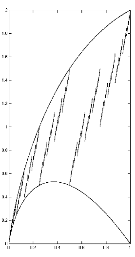
for $0\leq x\leq 1$.

Figure 1. Graphs of $y=H(x)$, $y=x\log_{2}(x)$, and $y=2x+\log_{2}(x)$

2.14 Proposition.

Let the function $H$ be extended from $[0,1)$ to ${\mathbf{R}}$ so that $H$ is periodic: $H(x+1)=H(x)$. Then $H$ satisfies the functional equation

(2.18) $$H(x)=\boldsymbol{\{}x\boldsymbol{\}}+\frac{1}{2}H(2x)$$

and thus $H$ has the series representation

(2.19) $$H(x)=\sum_{k=0}^{\infty}\frac{\boldsymbol{\{}2^{k}x\boldsymbol{\}}}{2^{k}}.$$

This implies $H$ is lower semi-continuous, continuous at all points of $[0,1]\setminus{\mathcal{D}}$ and right continuous at all points.

Proof.

This is a calculation based on the two series (2.17) and (2.16).

$$H(x) =\sum_{i=1}^{\infty}i\frac{r(2^{i}x)}{2^{i}}=\boldsymbol{\{}x\boldsymbol{\}}+\sum_{i=1}^{\infty}(i-1)\frac{r(2^{i}x)}{2^{i}}$$

$$=\boldsymbol{\{}x\boldsymbol{\}}+\frac{1}{2}\sum_{i=2}^{\infty}(i-1)\frac{r(2^{i-1}2x)}{2^{i-1}}$$

$$=\boldsymbol{\{}x\boldsymbol{\}}+\frac{1}{2}\sum_{j=1}^{\infty}j\frac{r(2^{j}2x)}{2^{j}}=\boldsymbol{\{}x\boldsymbol{\}}+\frac{1}{2}H(2x).$$

To prove the series representation (2.19) for $H(x)$ observe that an induction using the functional equation (2.18) yields

$$H(x)=\sum_{k=0}^{m}\frac{\boldsymbol{\{}2^{k}x\boldsymbol{\}}}{2^{k}}+\frac{1}{2^{m+1}}H(2^{m+1}x)$$

and as $0\leq H(x)\leq\sum_{i=1}^{\infty}i/2^{i}=2$ the series converges uniformly to $H(x)$. The functions $x\mapsto{\boldsymbol{\{}2^{k}x\boldsymbol{\}}}/{2^{k}}$ are lower semi-continuous and right continuous and hence so are the partial sums $S_{n}(x)=\sum_{k=0}^{n}{\boldsymbol{\{}2^{k}x\boldsymbol{\}}}/{2^{k}}$. Thus $H$ is the uniform limit of lower semi-continuous and right continuous functions and therefore is lower semi-continuous and right continuous. Finally the functions ${\boldsymbol{\{}2^{k}x\boldsymbol{\}}}/{2^{k}}$ are continuous at all points of $[0,1]\setminus{\mathcal{D}}$. As the series converges uniformly this implies that the sum $H$ is also continuous at these points. ∎

2.15 Remark.

The graph of $H(x)$ has an interesting “self-congruence” property. The series (2.19) for $H(x)$ implies for $m$ a positive integer that

$$H\Bigl{(}x+\frac{1}{2^{m}}\Bigr{)}=\sum_{k=0}^{m-1}\frac{1}{2^{k}}(\boldsymbol{\{}2^{k}x+2^{k-m}\boldsymbol{\}}-\boldsymbol{\{}2^{k}x\boldsymbol{\}})+H(x)=P_{m}(x)+H(x)$$

where this defines $P_{m}(x)$. It is not hard to check that the functions $(\boldsymbol{\{}2^{k}x+2^{k-m}\boldsymbol{\}}-\boldsymbol{\{}2^{k}x\boldsymbol{\}})/2^{k}$ are all constant on intervals $[i/2^{m},(i+1)/2^{m})$ and so the same will be true for $P_{m}(x)$. This implies for any $i$ and $j$ that the graph of the restriction $H\big{|}_{[i/2^{m},(i+1)/2^{m})}$ is a translation of the graph of $H\big{|}_{[j/2^{m},(j+1)/2^{m})}$. So informally and somewhat imprecisely “the graph of $H$ is locally self congruent at all the scales $1/2^{m}$”. If $F$ is the closure of the graph of $H\big{|}_{[0,1)}$ then this, and some calculation, can be used to show $F$ can be covered by $2^{m}$ closed sets of diameter $\leq 4m2^{-m}$. Thus for any $\delta>0$ the Hausdorff $\delta$-dimensional measure of $F$ is $\leq 2^{m}(4m2^{-m})^{\delta}$ and when $\delta>1$ we have $2^{m}(4m2^{-m})^{\delta}\to 0$ as $m\to\infty$. Therefore the Hausdorff dimension of $F$ is $\leq 1$. But as $F$ projects onto the interval $[0,1]$ its Hausdorff dimension is $\geq 1$. Thus $F$ has Hausdorff dimension one. (With a little more work it can be shown the one dimensional Hausdorff measure of $F$ is infinite.) However $F$ is compact, separable, totally disconnected and has no isolated points. Thus $F$ is homeomorphic to the Cantor set and therefore of topological dimension zero. Whence the closure of the graph of $F$ is a “fractal” in the sense that its geometric dimension is greater than its topological dimension.∎

2.16 Proposition.

The function $H$ is approximately sub-affine:

$$H\Bigl{(}\frac{x+y}{2}\Bigr{)}\leq\frac{H(x)+H(y)}{2}+\frac{x+y}{2}\quad\text{for}\quad x,y\in[0,1].$$

2.17 Lemma.

If $x=\sum_{i=0}^{N}{l_{i}}/{2^{i}}\in{\mathcal{D}}$ with each $l_{i}$ a nonnegative integer, then

$$H(x)\leq\sum_{i=0}^{N}i\frac{l_{i}}{2^{i}}$$

with equality if and only if each $l_{i}\in\{0,1\}$.

Proof.

If $(l_{0},l_{1},\dots,l_{N})$ is a finite sequence with $\sum_{i=0}^{N}{l_{i}}/{2^{i}}\leq 1$ we let $\lambda(l_{0},\dots,l_{N}):=\sum_{i=0}^{N}l_{i}$. The proof is by induction on $m=\lambda(l_{0},\dots,l_{N})$. If $m=0$ then each $l_{i}=0$ and $x=H(x)=0$ and the result is trivial. Now assume the inequality holds for all $(l_{0},l_{1},\dots,l_{N})$ with $\lambda(l_{0},\dots,l_{N})<m$. Let $k$ be the least integer such that $l_{k}\geq 2$ (if all $l_{k}\in\{0,1\}$ there is nothing to prove). Note $k\neq 0$ as $2/2^{0}=2$. Then

$$x =\sum_{i=0}^{k-2}\frac{l_{i}}{2^{i}}+\frac{l_{k-1}}{2^{k-1}}+\frac{l_{k}}{2^{k}}+\sum_{i=k+1}^{N}\frac{l_{i}}{2^{i}}$$

$$=\sum_{i=0}^{k-2}\frac{l_{i}}{2^{i}}+\frac{l_{k-1}+1}{2^{k-1}}+\frac{l_{k}-2}{2^{k}}+\sum_{i=k+1}^{N}\frac{l_{i}}{2^{i}}=\sum_{i=0}^{N}\frac{r_{i}}{2^{i}}$$

where the last line defines the $r_{i}$ implicitly. Then

$$\lambda(r_{0},\dots,r_{N})=\lambda(l_{0},\dots,l_{k-1}+1,l_{k}-2,\dots,l_{N})=\lambda(l_{0},\dots,l_{N})-1=m-1.$$

Thus the induction hypothesis gives

$$\sum_{i=0}^{N}i\frac{l_{i}}{2^{i}} =\sum_{i=0}^{N}i\frac{r_{i}}{2^{i}}+k\frac{2}{2^{k}}-(k-1)\frac{1}{2^{k-1}}$$

$$=\sum_{i=0}^{N}i\frac{r_{i}}{2^{i}}+\frac{k-(k-1)}{2^{k-1}}>\sum_{i=0}^{N}i\frac{r_{i}}{2^{i}}\geq H(x).$$

This gives $H(x)<\sum_{i=0}^{N}{l_{i}}/{2^{i}}$ unless $l_{i}\in\{0,1\}$ for all $i$. This completes the proof. ∎

Proof of Proposition 2.16.

First consider the case $x,y\in{\mathcal{D}}$ so that $x=\sum_{i=0}^{N}x_{i}/2^{i}$, $y=\sum_{i=0}^{N}y_{i}/2^{i}$. Then by Lemma 2.17

$$H\Bigl{(}\frac{x+y}{2}\Bigr{)} =H\bigg{(}\sum_{i=0}^{N}\frac{x_{i}+y_{i}}{2^{i+1}}\biggr{)}\leq\sum_{i=0}^{N}(i+1)\frac{x_{i}+y_{i}}{2^{i+1}}$$

$$=\frac{1}{2}\biggl{(}\sum_{i=0}^{N}i\frac{x_{i}}{2^{i}}+\sum_{i=1}^{N}i\frac{y_{i}}{2^{i}}\biggr{)}+\frac{1}{2}\biggl{(}\sum_{i=0}^{N}\frac{x_{i}}{2^{i}}+\sum_{i=1}^{N}\frac{y_{i}}{2^{i}}\biggr{)}$$

$$=\frac{H(x)+H(y)}{2}+\frac{x+y}{2}$$

If $x$ is a dyadic irrational and $y\in{\mathcal{D}}$ then we use that by Proposition 2.14 the function $H$ is lower semi-continuous on ${\mathbf{R}}$ and continuous at $x$. Let $x(r)\in{\mathcal{D}}$ so that $\lim_{r\to\infty}{x(r)}=x$ and so by continuity $\lim_{r\to\infty}H(x(r))=H(x)$. Thus

$$H\Bigl{(}\frac{x+y}{2}\Bigr{)} \leq\liminf_{r\to\infty}H\Bigl{(}\frac{x(r)+y}{2}\Bigr{)}\leq\lim_{r\to\infty}\left(\frac{H(x(r))+H(y)}{2}+\frac{x(r)+y}{2}\right)$$

$$=\frac{H(x)+H(y)}{2}+\frac{x+y}{2}$$

The case where both $x$ and $y$ are dyadic irrationals is handled similarly. ∎

2.18 Proposition.

Suppose $f$ is a lower semi-continuous approximately sub-affine function defined on $[0,1]$ such that $f(0)=0$. Then $f(x)\leq H(x)+f(1)x$ for all $x\in[0,1]$.

First some preliminaries. If $x=\sum_{j=1}^{N}x_{j}/2^{j}\in{\mathcal{D}}$ define the dyadic support of $x$ to be $\{j\in{\mathbf{N}}:x_{j}=1\}$ and denote it by $\operatorname{supp}\nolimits x$.

2.19 Lemma.

If $x,y\in{\mathcal{D}}$ and $(\operatorname{supp}\nolimits x)\cap(\operatorname{supp}\nolimits y)=\varnothing$ then

$$H\Big{(}\frac{x+y}{2}\Bigr{)}=\frac{H(x)+H(y)}{2}+\frac{x+y}{2}.$$

2.20 Remark.

This lemma motivated the definition of $H$. As the proof of Proposition 2.18 makes clear this is the property which implies $H$ is the largest lower semi-continuous approximately sub-affine function on $[0,1]$. It also allows one to compute the values of $H$ on ${\mathcal{D}}$ leading to the formula (2.15).∎

Proof.

The condition on the dyadic supports implies that the binary expansion of $x+y$ can be computed by just adding the digits without “carrying”. Thus for sufficiently large $N$

$$H\Bigl{(}\frac{x+y}{2}\Bigr{)} =\sum_{j=0}^{N}(j+1)\frac{x_{j}+y_{y}}{2^{j+1}}$$

$$=\frac{1}{2}\biggl{(}\sum_{j=0}^{N}(j+1)\frac{x_{j}}{2^{j}}+\sum_{j=0}^{N}(j+1)\frac{y_{j}}{2^{j}}\biggr{)}+\frac{x+y}{2}$$

$$=\frac{H(x)+H(y)}{2}+\frac{x+y}{2}.$$

∎

Proof of Proposition 2.18.

If $f(x)$ is replaced by $\varphi(x):=f(x)-f(1)x$ then $\varphi$ will also be approximately sub-affine and $\varphi(0)=\varphi(1)=0=H(0)=H(1)$. We now show by induction on $k$ that if $x=m/2^{k}\in{\mathcal{D}}$ then $\varphi(x)\leq H(x)$. The base case of $k=0$ holds. Now assume that $x=m/2^{k}$ and that the result is true when the denominator of the fraction is a smaller power of $2$. We may assume that $m$ is odd. If $x\leq 1/2$ let $y=2x=m/2^{k-1}$. Then $x=(0+y)/2$, $\varphi(y)\leq H(y)$ and $\operatorname{supp}\nolimits(0)\cap\operatorname{supp}\nolimits(y)=\varnothing$. Therefore

$$\varphi(x) =\varphi\Bigr{(}\frac{0+y}{2}\Bigr{)}\leq\frac{\varphi(0)+\varphi(y)}{2}+\frac{0+y}{2}$$

$$\leq\frac{H(0)+H(y)}{2}+\frac{0+y}{2}=H\Bigl{(}\frac{0+y}{2}\Bigr{)}=H(x).$$

If $1/2<x<1$ then let $y=2x-1$ so that $x=(y+1)/2$. Then as the dyadic supports of $y$ and $1$ are disjoint, a calculation like the one just done shows $\varphi(x)\leq H(x)$. Thus $\varphi(x)\leq H(x)$ for all $x\in{\mathcal{D}}$. For any other $x\in[0,1]\setminus{\mathcal{D}}$ choose $x_{k}\in{\mathcal{D}}$ with $x_{k}\to x$. By Proposition 2.14 $H$ is continuous at $x$. Therefore the lower semi-continuity of $\varphi$ implies

$$\varphi(x)\leq\liminf_{k\to\infty}\varphi(x_{k})\leq\lim_{k\to\infty}H(x_{k})=H(x).$$

Finally $\varphi(x)\leq H(x)$ is equivalent to the required inequality for $f$. ∎

2.21 Proposition.

The inequalities

(2.20) $$x\log_{2}(1/x)\leq H(x)\leq 2x+\log_{2}(1/x)$$

hold for $0\leq x\leq 1$ (cf. Figure 1).

2.22 Lemma.

Let $\varphi(x):=x\log_{2}(1/x)=-x\ln(x)/\ln(2)$. Then for $0\leq t\leq 1$ and $x,y\in[0,1]$

$$0\leq\varphi((1-t)x+tx)-t\varphi(x)-(1-t)\varphi(x)\leq\varphi(t)x+\varphi(1-t)y.$$

As $\varphi(1/2)=1/2$ this implies $\varphi$ is approximately sub-affine on $[0,1]$.

Proof.

The left hand inequality follows from the concavity of $\varphi$. To prove the right hand inequality we first assume $0<x\leq y\leq 1$. For fixed $t$ and $y$ let

$$F(x):=\varphi((1-t)x+ty)-(1-t)\varphi(x)-t\varphi(y).$$

Then

$$F^{\prime}(x)=\frac{(1-t)}{\ln(2)}(\ln(x)-\ln((1-t)x+ty))\leq 0.$$

Therefore $F$ is monotone decreasing and so the maximum of $F(x)$ on $[0,y]$ occurs when $x=0$. But

$$F(0)=\varphi(ty)-t\varphi(y)=\frac{-(ty\ln(ty)-ty\ln(y))}{\ln(2)}=\frac{-t\ln(t)}{\ln(2)}\,y=\varphi(t)y.$$

So for all $0\leq x\leq y$ and $0\leq t\leq 1$

$$\varphi((1-t)x+ty)-t\varphi(x)-(1-t)\varphi(y)\leq\varphi(t)y\leq\varphi(t)y+\varphi(1-t)x$$

(for the last step note that $\varphi(1-t)x\geq 0$). A similar argument works in the case $y\leq x$ (or replace $t$ by $(1-t)$ in what has been shown). ∎

Proof of Proposition 2.21.

As the function $\varphi(x)=x\log_{2}(1/x)$ is approximately sub-affine, vanishes at the endpoints of $[0,1]$ and is continuous the lower bound of (2.20) follows from Proposition 2.18. To prove the upper bound we use the series (2.19). Let $0<x<1$. There exists a unique nonnegative integer $m$ so that $2^{m}x<1\leq 2^{m+1}x$ (i.e. $1/2^{m+1}\leq x<1/2^{m}$). Then for $0\leq k\leq m$ we have $\boldsymbol{\{}2^{k}x\boldsymbol{\}}=2^{k}x$, and thus

$$H(x)=\sum_{k=0}^{\infty}\frac{1}{2^{k}}\boldsymbol{\{}2^{k}x\boldsymbol{\}}\leq(m+1)x+\sum_{k=m+1}^{\infty}\frac{1}{2^{k}}=(m+1)x+\frac{1}{2^{m}}.$$

So to complete the proof it is enough to show

$$\psi(x):=2x+x\log_{2}(1/x)-\Bigl{(}(m+1)x+\frac{1}{2^{m}}\Bigr{)}=\frac{-x\ln(x)}{\ln(2)}-(m-1)x+\frac{1}{2^{m}}$$

satisfies $\psi(x)\geq 0$ for $x\in[1/2^{m+1},1/2^{m}]$. But $\psi(1/2^{m+1})=\psi(1/2^{m})=0$ and $\psi^{\prime\prime}(x)=-1/(x\ln(2))<0$. So $\psi$ is concave on $[1/2^{m+1},1/2^{m}]$ and vanishes at the endpoints which implies $\psi\geq 0$ on the interval. ∎

2.4. The extremal approximately convex function $E(x)$ on a simplex

Let $e_{0},\dots,e_{n}$ be the standard basis of ${\mathbf{R}}^{n+1}$. Then the standard simplex is, as usual, $\Delta_{n}=\operatorname{Co}\nolimits\{e_{0},\dots,e_{n}\}$. We will often write points of $\Delta_{n}$ in terms of their affine coordinates $(x_{0},\dots,x_{n})$ where $x_{k}\geq 0$ and $\sum_{k=0}^{n}x_{k}=1$. This corresponds to $\sum_{k=0}^{n}x_{k}e_{k}$. Define a function $E$ on $\Delta_{n}$ as follows:

(2.21) $$E\biggl{(}\sum_{k=0}^{n}x_{k}e_{k}\biggr{)}=E(x_{0},\dots,x_{n}):=\sum_{k=0}^{n}H(x_{k}).$$

2.23 Remark.

If $\mu$ is a finite measure space and $\mathcal{A}$ is a finite algebra of measurable sets with atoms $A_{0},A_{1},\dots,A_{n}$ the entropy of $\mathcal{A}$ is $-\sum_{k=0}^{n}\mu(A_{k})\ln\mu(A_{k})$. If $x\in\Delta_{n}$ we can think of $x$ as a measure on $\{0,1,,\dots,n\}$. If $\mathcal{A}$ is the algebra of subsets of $\{0,1,,\dots,n\}$ then its entropy with respect to the measure determined by $x$ is $-\sum_{x_{k}}^{n}x_{k}\ln x_{k}$. By Lemma 2.22 the function $x\log_{2}(1/x)$ is approximately sub-affine and so $H$ can be viewed as an extremal version of $x\log_{2}(1/x)$. To the extent that $H(x)$ and $-x\ln(x)$ can be thought of as analogous functions, $E(x)=\sum_{k=0}^{n}H(x_{k})$ can be viewed as a “poor man’s” version of the entropy. The inequalities 2.20 make this analogy somewhat precise. ∎

The standard dyadic simplex is

$${\mathcal{D}}_{n}:=\biggl{\{}\sum_{k=0}^{n}x_{k}e_{k}:x_{k}\in{\mathcal{D}},\ \sum_{k=0}^{n}x_{k}=1\biggr{\}}.$$

Like ${\mathcal{D}}\subset[0,1]$ the set ${\mathcal{D}}_{n}$ will play a large rôle.

2.24 Proposition.

The function $E$ is approximately convex and lower semi-continuous on $\Delta_{n}$ with $E(e_{k})=0$ for $0\leq k\leq n$. The points of continuity of $E$ are the points $x=(x_{0},\dots,x_{n})$ such that all the coordinates $x_{k}$ are dyadic irrationals. Moreover $E$ satisfies the inequalities

$$\sum_{k=0}^{n}x_{k}\log_{2}(1/x_{k})\leq E(x_{0}e_{0}+\cdots+x_{n}e_{n})\leq 2+\sum_{k=0}^{n}x_{k}\log_{2}(1/x_{k}).$$

Proof.

For $x\in\Delta_{n}$ the functions $x\mapsto H(x_{k})$ are lower semi-continuous by Proposition 2.14. Thus $E$ will also be lower semi-continuous. Also from Proposition the points of continuity of $H$ are the dyadic irrationals in $[0,1]$. This implies the statement about the points of continuity of $E$. As $H$ is approximately sub-affine we have

$$E\Bigl{(}\frac{x+y}{2}\Bigr{)} =\sum_{k=0}^{n}H\Bigl{(}\frac{x_{k}+y_{k}}{2}\Bigr{)}$$

$$\leq\sum_{k=0}^{n}\frac{H(x_{k})+H(y_{k})}{2}+\sum_{k=0}^{n}\frac{x_{k}+y_{k}}{2}$$

$$=\frac{E(x)+E(y)}{2}+1$$

as $\sum_{k=0}^{n}x_{k}=\sum_{k=0}^{n}y_{k}=1$. So $E$ is approximately convex as claimed. That $E(e_{k})=0$ follows from $H(0)=H(1)=0$. The bounds for $E$ follow from the inequalities (2.20). ∎

It is possible to give an explicit formula for $E$ on the one dimensional simplex.

2.25 Proposition.

Let the one dimensional simplex $\Delta_{1}$ be identified with $[0,1]$ in the usual manner ($t$ corresponds to $(1-t)e_{0}+te_{1}$). Then

(2.22) $$E(t)=\begin{cases}2,&t\notin{\mathcal{D}};\\ 2-\dfrac{1}{2^{l-1}},&\dfrac{m}{2^{l}}\in{\mathcal{D}}\text{ with $m$ odd}.\end{cases}$$

Proof.

Set $\psi(t)=\boldsymbol{\{}t\boldsymbol{\}}+\boldsymbol{\{}1-t\boldsymbol{\}}=\boldsymbol{\{}t\boldsymbol{\}}+\boldsymbol{\{}-t\boldsymbol{\}}$. Then by (2.19)

(2.23) $$E(t)=H(t)+H(1-t)=\sum_{k=0}^{\infty}\frac{\psi(2^{k}t)}{2^{k}}.$$

But then $\psi(t)=0$ for $t\in\mathbf{Z}$ and $\psi(t)=1$ for $t\notin\mathbf{Z}$. So if $t\notin{\mathcal{D}}$ we have $\psi(2^{k}t)=1$ for all $k$. If $t=m/2^{l}$ with $m$ odd then $\psi(2^{k}t)=1$ for $k<l$ and $\psi(2^{k}t)=0$ for $k\geq l$. Now the required formula for $E(t)$ follows from the series (2.23). ∎

Unfortunately, in higher dimensions $E$ is not as easy to understand. A graph of $E$ on the two dimensional simplex is shown in Figure 2.

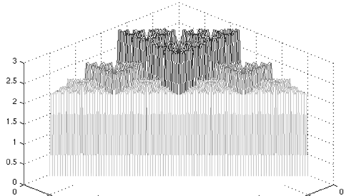
Figure 2. Graph of $z=E(x,y,1-x-y)$ for $0\leq x\leq 1-y\leq 1$
                 $\ldots$ tum Tartarus ipse Then Tartarus itself goes plunging down bis patet in praeceps tantum tenditque sub umbras In darkness twice as deep as heaven is high quantus ad aetherium caeli suspectus Olympum For eyes fixed on etherial Olympus                  $\cdots$                  $\cdots$ Respicit Aeneas subito et sub rupe sinistra The Heroe, looking on the left, espy’d moenia lata videt triplici circumdata muro A lofty Tow’r, and strong on ev’ry side quae rapidis flammis ambit torrentibus amnis With treble Walls, which Phlegethon surrounds, Tartareus Phlegethon, torquetque Whose fiery flood the burning empire bounds: sonantia saxa And press’d betwixt the Rocks, the bellowing noise resounds. Vergil, The Aeneid Translations by Robert Fitzgerald and John Dryden

2.26 Remark.

The graph (Figure 2) of $E$ suggests that $E$ has some self similarities. This is indeed the case as we now briefly indicate. For each $k\in\{0,\dots,n\}$ define a map $\theta_{k}\colon\Delta_{n}\to\Delta_{n}$ by

$$\theta_{k}(x):=\frac{e_{k}+x}{2}$$

This is the dilation by a factor of $1/2$ centered at $e_{k}$ and it maps $\Delta_{n}$ onto its subset defined by $1/2\leq x_{k}\leq 1$. The functional equation (2.18) for $H$ can be rewritten in the from $H(t/2)=\boldsymbol{\{}t/2\boldsymbol{\}}+\frac{1}{2}H(t/2)$. We leave it as an exercise for the reader to show this (and $H(t+1/2)=H(t)+1/2$ for $0<t<1/2$) can be used in the definition of $E$ so show that for any $x\in\Delta_{n}$ which is not a vertex that

$$E(\theta_{k}(x))=1+\frac{1}{2}E(x).$$

Thus if on the space $\Delta_{n}\times[0,\infty)$ a map $\Theta_{k}$ is defined by $\Theta_{k}(x,z)=\bigl{(}\theta_{k}(x),1+z/2\bigr{)}$ then the graph of $E$ (with the points over the vertices deleted) is invariant under $\Theta_{k}$. Each $\Theta_{k}$ is the dilation by a factor of $1/2$ with center $(e_{k},2)$. This explains the self similarities of the graph of $E$.∎

Our next result implies that the upper bound of Theorem 2.3 is sharp. Recall that a subset of a metric space is a $G_{\delta}$ iff it is a countable intersection of open sets.

2.27 Theorem.

The function $E$ achieves its maximum value of $\kappa(n)$ on an uncountable $G_{\delta}$ subset of $\Delta_{n}$.

2.28 Remark.

The maximum of $E$ does not occur at the center $(1/(n+1),\dots,1/(n+1))$ of $\Delta_{n}$. Given the symmetry of the problem this is a little surprising.∎

Proof.

That $\sup E[\Delta_{n}]\leq\kappa(n)$ follows from 2.3. To show the maximum is obtained, let $m=[\log_{2}(n)]$ so that $n=2^{m}+r$ with $0\leq r<2^{m}$. Suppose $x=(x_{0},\dots,x_{n})\in\Delta_{n}$ with each coordinate $x_{k}$ a dyadic irrational. In particular, if $x_{k}=\sum_{j=0}^{n}x_{kj}/2^{j}$ then $x_{kj}$ is zero for infinitely many $j$ and one for infinitely many $j$. Let $M_{j}(x):=\#\{k:x_{kj}=1\}$. We claim that $E(x)=\kappa(n)$ provided each coordinate $x_{k}$ is a dyadic irrational and

(2.24) $$M_{j}(x)=\begin{cases}0,&j\leq m;\\ n-2r,&j=m+1;\\ n,&j\geq m+2.\end{cases}$$

Let $K$ be the set of all $x=(x_{0},\dots,x_{n})$ that satisfy these two conditions. If $x\in K$, then

$$\sum_{k=0}^{n}x_{k}=\sum_{j=0}^{\infty}\sum_{k=0}^{n}\frac{x_{kj}}{2^{j}}=\frac{M_{m+1}}{2^{m+1}}+n\sum_{j=m+2}^{\infty}\frac{1}{2^{j}}=\frac{n-2r}{2^{m+1}}+\frac{n}{2^{m+1}}=\frac{n-r}{2^{m}}=1$$

Thus $x\in\Delta_{n}$ and so $K\subset\Delta_{n}$.

To see that $K$ is uncountable (and thus nonempty) let $\langle a_{m+2},a_{m+3},\dots\rangle$ be a sequence in $\{0,1,\dots,n\}$ such that for every $k\in\{0,1,\dots,n\}$, $a_{j}=k$ for infinitely many $j$. We let $x_{kj}=0$ if $j\leq m$ and we let $x_{k\,\,m+1}=1$ for exactly $n-r$ many $k$. For $j\geq m+2$, let

$$x_{kj}:=\begin{cases}1,&a_{j}\neq j;\\ 0,&a_{j}=k.\end{cases}$$

Since each sequence $\langle x_{kj}\rangle_{j=0}^{\infty}$ has infinitely many zeros and ones, each $x_{k}$ is a dyadic irrational. Thus $x=(x_{0},\dots,x_{n})\in K$. As there are uncountably many such sequences $\langle a_{m+2},a_{m+3},\dots\rangle$ the set $K$ is uncountable.

If $x=(x_{0},\dots,x_{n})\in K$ then, using the definition (2.15) of $H$ and the identity $\sum_{j=m+2}^{\infty}{j}/{2^{j}}=(m+3)/2^{m+1}$, we have

$$E(x) =\sum_{k=0}^{n}H(x_{k})=\sum_{j=0}^{\infty}\frac{jM_{j}}{2^{j}}=\frac{M_{m+1}(m+1)}{2^{m+1}}+n\sum_{j=m+2}^{\infty}\frac{j}{2^{j}}$$

$$=\frac{(n-2r)(m+1)}{2^{m+1}}+\frac{n(m+3)}{2^{m+1}}=\frac{(2n-2r)(m+1)+2n}{2^{m+1}}$$

$$=m+1+\frac{n}{2^{m}}=\kappa(n).$$

This shows that $E$ achieves its maximum at all points of $K$. Finally $\{x\in\Delta_{n}:E(x)=\kappa(n)\}=\bigcap_{\ell=1}^{\infty}E^{-1}\big{[}(\kappa(n)-1/\ell,\infty)\big{]}$ and each of the sets $E^{-1}\big{[}(\kappa(n)-1/\ell,\infty)\big{]}$ is open as $E$ is lower semi-continuous. Thus $\{x\in\Delta_{n}:E(x)=\kappa(n)\}$ is a $G_{\delta}$. ∎

2.29 Remark.

With a little more work it can be shown that $E(x)=\kappa(n)$ if and only if $x\in K$ with $K$ as above.∎

2.30 Theorem.

The function $E$ is the largest bounded approximately convex function on $\Delta_{n}$ that vanishes on the vertices. More precisely, if $h$ is any bounded approximately convex function on $\Delta_{n}$ with $h(e_{k})\leq 0$ for $k=0,1,\dots,n$, then $h\leq E$ on $\Delta_{n}$.

2.31 Corollary.

Let $h\colon\Delta_{n}\to{\mathbf{R}}$ be an approximately convex function that is Borel measurable. Then for any $x=\sum_{k=0}^{n}x_{k}e_{k}$ the inequality

$$h(x)\leq\kappa(n)+\sum_{k=0}^{n}x_{k}h(e_{k})$$

holds. In particular, if $h(e_{k})\leq 0$ for all $k$, then $h\leq\kappa(n)$.

Proof of Theorem 2.31.

Define $l$ on $\Delta_{n}$ by $l(x)=\sum_{k=0}^{n}x_{k}h(e_{k})$. Then the function $h(x)-l(x)$ is approximately convex, Borel measurable, and vanishes on the vertices of $\Delta_{n}$. So by replacing $h$ by $h-l$ we may assume $h$ vanishes on the vertices of $\Delta_{n}$ it will be enough to show $h\leq\kappa(n)$ on $\Delta_{n}$. We do this by induction on $n$. For $n=1$ it follows from results of Ng and Nikodem [5, Cor. 1 and Thm 2] that $h$ is bounded above. But then $h\leq\kappa(1)=2$ by Theorem 2.3. Now let $n\geq 2$ and assume the result holds for all simplices with dimension $<n$. Consider $\Delta_{n-1}$ as a face of $\Delta_{n}$ in the natural way ($\Delta_{n-1}=\operatorname{Co}\nolimits\{e_{0},\dots,e_{n-1}\}\subset\operatorname{Co}\nolimits\{e_{0},\dots,e_{n}\}$). Then by the induction hypothesis $h\big{|}_{\Delta_{n-1}}\leq\kappa(n-1)$. Now any point $x\in\Delta_{n}$ has a representation as $x=(1-t)e_{n}+ty$ where $y\in\Delta_{n-1}$ and $t\in[0,1]$. But then the one dimensional result (applied to the restriction of $h$ to the segment between $e_{0}$ and $y$ where we note that this restriction is Borel and thus Lebesgue measurable) implies

$$h(x) =h((1-t)e_{n}+ty)\leq 2+(1-2)h(e_{n})+th(y)$$

$$\leq 2+0+t\kappa(n-1)\leq 2+\kappa(n-1).$$

Thus $h$ is bounded above on $\Delta_{n}$. But then we can use Theorem 2.3 and reduce the bound to $\kappa(n)$. This completes the proof. ∎

2.32 Corollary.

Let $U\subseteq{\mathbf{R}}^{n}$ be a convex set and let $h\colon U\to{\mathbf{R}}$ be either Borel measurable or bounded above on compact subsets of $U$. Then for any $m\leq n$, points $x_{0},\dots,x_{m}\in U$ and $(\alpha_{0},\dots,\alpha_{m})\in\Delta_{m}$, we have

$$h(\alpha_{0}x_{0}+\cdots+\alpha_{m}x_{m}) \leq E(\alpha_{0},\dots,\alpha_{m})+\alpha_{0}h(x_{0})+\cdots+\alpha_{m}h(x_{m})$$

$$\leq\kappa(m)+\alpha_{0}h(x_{0})+\cdots+\alpha_{m}h(x_{m}).$$

Proof.

Define $f\colon\Delta_{m}\to{\mathbf{R}}$ by $f(\alpha_{0},\dots,\alpha_{m}):=h(\alpha_{0}x_{0}+\cdots+\alpha_{m}x_{m})-\big{(}\alpha_{0}h(x_{0})+\cdots+\alpha_{m}h(x_{m})\big{)}$. Then $f$ is approximately convex and bounded above on $\Delta_{m}$ or is Borel measurable on $\Delta_{m}$. As $f$ vanishes on the vertices of $\Delta_{m}$ either Theorem 2.30 or Corollary 2.31 implies $f\leq E\leq\kappa(m)$ on $\Delta_{m}$. This is equivalent to the conclusion of the corollary. ∎

We start the proof of Theorem 2.30 by extending the idea of the dyadic support from ${\mathcal{D}}$ to ${\mathcal{D}}_{n}$. If $x=\sum_{k=0}^{n}\left(\sum_{j=0}^{N}x(j,k)/2^{j}\right)e_{k}\in{\mathcal{D}}_{n}$ (here $x(j,k)\in\{0,1\}$) then set

(2.25) $$\operatorname{supp}\nolimits x:=\{(j,k):x(j,k)=1\}.$$

The following is trivial to prove using Lemma 2.19 and the definition of $E$ in terms of $H$.

2.33 Lemma.

If $x,y\in{\mathcal{D}}_{n}$ and $(\operatorname{supp}\nolimits x)\cap(\operatorname{supp}\nolimits y)=\varnothing$ then

$$E\Bigl{(}\frac{x+y}{2}\Bigr{)}=\frac{E(x)+E(y)}{2}+1.$$

∎

2.34 Lemma.

If $x\in{\mathcal{D}}_{n}$ and $x\notin\{e_{0},\dots,e_{n}\}$, then there are $y,z\in{\mathcal{D}}_{n}$ so that $x=(y+z)/2$ and $(\operatorname{supp}\nolimits y)\cap(\operatorname{supp}\nolimits z)=\varnothing$.

Proof.

Letting $x=\sum_{k=0}^{n}\left(\sum_{j=0}^{N}x(j,k)/2^{k}\right)e_{k}$ It suffices to show that there are nonempty sets $A$, $B$ so that $A\cap B=\varnothing$ and

$$\sum_{(j,k)\in A}\frac{x(k,j)}{2^{j}}=\frac{1}{2}=\sum_{(j,k)\in B}\frac{x(k,j)}{2^{j}}.$$

For then if $a=\sum_{(j,k)\in A}{x(k,j)}/{2^{j-1}}e_{k}$ and $b=\sum_{(j,k)\in B}{x(k,j)}/{2^{j-1}}e_{k}$ we have $a,b\in{\mathcal{D}}_{n}$, $(\operatorname{supp}\nolimits a)\cap(\operatorname{supp}\nolimits b)=\varnothing$ and $x=(a+b)/2$.

We first prove by induction on $\sum_{j=1}^{N}a_{j}$ that if $a_{1},\dots,a_{N}$ are positive integers so that $\sum_{j=1}^{N}a_{j}/2^{j}=1$ then there are $b_{j},c_{j}\in{\mathbf{N}}$ such that $\sum_{j=1}^{N}b_{j}/2^{j}=\sum_{j=1}^{N}c_{j}/2^{j}=1/2$. Note that $a_{N}$ is even (otherwise $2^{-N}\sum_{j=1}^{N}2^{N-j}a_{j}$ would not sum to $1$) and so $a_{N}-2\geq 0$. Therefore

$$\sum_{j=1}^{N-2}\frac{a_{j}}{2^{j}}+\frac{a_{N-1}+1}{2^{N-1}}+\frac{a_{N}-2}{2^{N}}=1.$$

Since $\sum_{j=1}^{N-2}+(a_{N-1}+1)+(a_{N}-2)=\sum_{j=1}^{N}a_{j}-1$ we may apply the induction hypothesis, which yields the claim.

Now let $x\in{\mathcal{D}}_{n}$ be as above. Let $a_{j}:=\#\{k:x(j,k)=1\}$. Then $\sum_{j=1}^{N}a_{j}/2^{j}=1$. Therefore we have $a_{j}=b_{j}+c_{j}$ as above. Then splitting each of the sets $\{k:x(j,k)=1\}$ into two disjoint sets $A_{j}$ and $B_{j}$ with $\#(A_{j})=b_{j}$ and $\#(B_{j})=c_{j}$ we let $A:=\cup_{j=1}^{N}A_{j}$ and $B:=\cup_{j=1}^{N}B_{j}$. This completes the proof. ∎

2.35 Proposition.

Let $h$ be any approximately convex function on $\Delta_{n}$ (not necessarily bounded above) such that $h(e_{k})\leq 0$ for $0\leq k\leq n$. Then $h(x)\leq E(x)$ for all $x\in{\mathcal{D}}_{n}$.

Proof.

The proof is by induction on $m=\#(\operatorname{supp}\nolimits x)$. If $m=1$ then $x=e_{k}$ for some $k$ and $h(e_{k})\leq 0=E(e_{k})$. Now assume that $h(x)\leq E(x)$ for all $x$ with $\#(\operatorname{supp}\nolimits x)\leq m-1$ and let $\operatorname{supp}\nolimits x=m$. By Lemma 2.34 we can write $x=(y+z)/2$ with $\#(\operatorname{supp}\nolimits y),\#(\operatorname{supp}\nolimits z)\leq m-1$. Using the induction hypothesis and Lemma 2.33

$$h(x)=h\Bigl{(}\frac{y+z}{2}\Bigr{)}\leq\frac{h(y)+h(z)}{2}+1\leq\frac{E(y)+E(z)}{2}+1=E(x).$$

∎

The following lets us pass from knowing inequalities for $E$ on ${\mathcal{D}}_{n}$ to proving them on $\Delta_{n}$.

2.36 Lemma.

If $x\in\Delta_{n}$ then there is a sequence $\langle x(r)\rangle_{r=1}^{\infty}$ from ${\mathcal{D}}_{n}$ so that $\lim_{r\to\infty}x(r)=x$ and $\lim_{r\to\infty}E(x(r))=E(x)$.

Proof.

Write $x=\sum_{k=0}^{n}x_{k}e_{k}$. By reordering we can assume for some $\ell\in\{0,\dots,n\}$ that $x_{k}\in{\mathcal{D}}$ for $0\leq k\leq\ell$ and $x_{k}\notin{\mathcal{D}}$ for $\ell+1\leq k\leq n$. For $0\leq k\leq\ell$ set $x_{k}(r)=x_{k}$ for all $r$. As $\sum_{k=0}^{n}x_{k}=1$ and $\sum_{k=0}^{\ell}x_{k}\in{\mathcal{D}}$ (as $x_{k}\in{\mathcal{D}}$ for each $x_{k}$ in this sum) the sum $\delta:=\sum_{k=\ell+1}^{n}x_{k}=1-\sum_{k=0}^{\ell}x_{k}$ will also be a dyadic rational. Let $\Delta_{n-\ell-1}(\delta)=\{\sum_{k=\ell+1}^{n}\alpha_{k}e_{k}:\alpha_{k}\geq 0,\sum_{k=\ell+1}^{n}\alpha_{k}=\delta\}$ and ${\mathcal{D}}_{n-\ell-1}(\delta)=\{\sum_{k=\ell+1}^{n}\alpha_{k}e_{k}:\alpha_{k}\in{\mathcal{D}},\sum_{k=\ell+1}^{n}\alpha_{k}=\delta\}$. Then ${\mathcal{D}}_{n-\ell-1}(\delta)$ will be dense in $\Delta_{n-\ell-1}(\delta)$ so there is a sequence $y(r)=\sum_{k=\ell+1}^{n}y_{k}(r)e_{k}$ with $\lim_{r\to\infty}y(r)=y$. Set $x_{k}(r)=y_{k}(r)$ for $\ell+1\leq k\leq n$. Then $x_{k}(r)=x_{k}\in{\mathcal{D}}$ for $0\leq k\leq\ell$ and $\lim_{r\to\infty}x_{k}(r)=x_{k}\notin{\mathcal{D}}$ for $\ell+1\leq k\leq n$. Set $x(r)=\sum_{k=0}^{n}x_{k}(r)e_{k}$. Then $x(r)\in{\mathcal{D}}_{n}$ and $\lim_{r\to\infty}x(r)=x$. We now use the definition of $E$ in terms of $H$ and the fact that $H$ is continuous at all dyadic irrationals (Proposition 2.14) to obtain

$$\lim_{r\to\infty}E(x(r))=\sum_{k=0}^{\ell}H(x_{k})+\lim_{r\to\infty}\sum_{k=\ell+1}^{n}H(x_{k}(r))=\sum_{k=0}^{n}H(x_{k})=E(x).$$

∎

Proof of Theorem 2.30.

Let $E_{\Delta_{n},0}$ extremal approximately convex function on $\Delta_{n}$ that takes the values $0$ on the vertices (cf. (2.3)). We wish to show $E=E_{\Delta_{n},0}$. The inequality $E\leq E_{\Delta_{n},0}$ follows from the definition of $E_{\Delta_{n},0}$, so it is enough to prove $E_{\Delta_{n},0}\leq E$. By Lemma 2.36 there is a sequence $x(r)\in{\mathcal{D}}_{n}$ such that $\lim_{r\to\infty}x(r)=x$ and $\lim_{r\to\infty}E(x(r))=E(x)$. By Lemma 2.35 $E_{\Delta_{n},0}(x(r))\leq E(x(r))$. By Theorem 2.12 the function $E_{\Delta_{n},0}$ is lower semi-continuous. Therefore

$$E_{\Delta_{n},0}(x)\leq\liminf_{r\to\infty}E_{\Delta_{n},0}(x(r))\leq\lim_{r\to\infty}E(x(r))=E(x).$$

∎

2.5. Extremal approximately convex functions on convex polytopes

Let $K\subset{\mathbf{R}}^{n}$ be a compact convex set with extreme points $V$ and let $\varphi\colon V\to{\mathbf{R}}$ be bounded. In §2.2 we defined the extremal approximately convex function $E_{K,\varphi}$ with extreme values $\varphi$ but without being explicit about how to compute it. In §2.4 we gave a very explicit description of $E=E_{\Delta_{n},0}$, the extremal approximately convex function on the simplex. Here we show that when $K$ is a polytope (that is the convex hull of a finite number of points) then $E_{K,\varphi}$ can be expressed directly in terms of $E_{\Delta_{m},0}$ for some $m$. We first establish some elementary properties of approximately convex functions under affine maps.

2.37 Proposition.

Let $A\subset{\mathbf{R}}^{m}$ and $B\subset{\mathbf{R}}^{n}$ be convex sets and $T\colon{\mathbf{R}}^{m}\to{\mathbf{R}}^{n}$ an affine map.

1. If $T[A]\subseteq B$ and $f$ is an approximately convex function on $B$ then $T^{*}f(x):=f(T(x))$ is an approximately convex function on $A$.

2. If $T[A]\supseteq B$ and $h$ is an approximately convex function on $A$ which is bounded from below then $T_{*}h(y):=\inf_{T(x)=y}h(x)$ is approximately convex on $B$.

3. Both $T^{*}$ and $T_{*}$ are order preserving. That is $f_{1}\leq f_{2}$ and $h_{1}\leq h_{2}$ pointwise implies $T^{*}f_{1}\leq T^{*}f_{2}$ and $T_{*}h_{1}\leq T_{*}h_{2}$ pointwise.

4. If $T[A]=B$, $h$ is approximately convex and bounded below on $A$ and $f$ is approximately convex and bounded below on $B$, then $T^{*}T_{*}h\leq h$ and $T_{*}T^{*}f=f$.

Proof.

This is just a chase through the definitions of $T^{*}$ and $T_{*}$. ∎

Let $K$ be a convex polytope in ${\mathbf{R}}^{n}$ with extreme points $V=\{v_{0},\dots,v_{m}\}$ and extreme values given by $\varphi\colon V\to{\mathbf{R}}$. and let $a_{0},\dots,a_{m}$ be real numbers. We wish to find the largest approximately convex function $F$ on $K$ so that $F(v_{k})=\varphi(v_{k})$ for $0\leq k\leq m$. Toward this end let $E=E_{\Delta_{m},0}$ be the extremal approximately convex function on the simplex $\Delta_{m}$ and define $E_{\Delta_{m},\varphi}$ on $\Delta_{M}$ by

$$E_{\Delta_{m},\varphi}(x)=E_{\Delta_{m},\varphi}(x_{0},\dots,x_{m}):=E_{\Delta_{m},0}(x_{0},\dots,x_{m})+\sum_{k=0}^{m}x_{k}\varphi(a_{k}).$$

(This is a slight misuse of notation as $\varphi$ is a function on the extreme points $V$ of $K$ rather than the set of extreme points $\{e_{0},\dots,e_{m}\}$ of $\Delta_{m}$.) Then, as $x\mapsto\sum_{k=0}^{m}x_{k}a_{k}$ is affine, the function $E_{\Delta_{m},\varphi}$ is approximately convex on $\Delta_{m}$ and satisfies $E_{\Delta_{m},\varphi}(e_{k})=\varphi(v_{k})$. Moreover $E_{\Delta_{m},\varphi}$ is the extremal approximately convex function on $\Delta_{m}$ taking on these values on the vertices in the sense that if $f\colon\Delta_{m}\to{\mathbf{R}}$ is approximately convex and bounded above, lower semi-continuous, and $f(e_{k})\leq\varphi(v_{k})$ then $f(x)\leq E_{\Delta_{m},\varphi}(x)$ for all $x\in\Delta_{m}$.

Returning to our extremal problem there is a unique affine map $T\colon\Delta_{m}\to K$ such that $T(e_{k})=v_{k}$ for $0\leq k\leq m$. Then $T[\Delta_{m}]=K$. Define $F_{K,}\colon K\to{\mathbf{R}}$ by

$$F_{K,\varphi}:=T_{*}E_{\Delta_{m},\varphi}.$$

Then another definition chase shows $F_{K,\varphi}(v_{k})=a_{k}$.

2.38 Theorem.

Using the notation above, the extremal approximately continuous function on the polytope $K$ with extreme values $\varphi$ is

$$E_{K,\varphi}:=T_{*}E_{\Delta_{0},\varphi}.$$

The function $E_{K,\varphi}$ is lower semi-continuous.

Proof.

Let $f\colon K\to{\mathbf{R}}$ be approximately convex, bounded, and and satisfy $f(v_{k})\leq\varphi(v_{k})$. Then the function $T^{*}f$ on $\Delta_{m}$ is approximately convex, bounded, and $T^{*}f(e_{k})=f(v_{k})\leq\varphi(v_{k})$. Therefore $T^{*}f\leq E_{\Delta_{m},\varphi}$. But then $f=T_{*}T^{*}f\leq T_{*}E_{\Delta_{m},\varphi}$ which proves $T_{*}E_{\Delta_{m},\varphi}=E_{K,\varphi}$. The lower semi-continuity of $E_{K,\varphi}$ follows from Theorem 2.12. ∎

2.6. A stability theorem of Hyers-Ulam type

Here we give a stability result for approximately convex functions related to and motivated by a theorem of Hyers and Ulam [4]. The idea is that an approximately convex function is close (in the uniform norm) to some convex function.

2.39 Theorem.

Assume that $U\subseteqq{\mathbf{R}}^{n}$ is convex, $\varepsilon>0$, and that $f\colon U\to{\mathbf{R}}$ is bounded above on compact sets and satisfies

(2.26) $$f\Bigl{(}\frac{x+y}{2}\Bigr{)}\leq\frac{f(x)+f(y)}{2}+\varepsilon.$$

Then there exist convex functions $g,g_{0}\colon U\to{\mathbf{R}}$ such that

(2.27) $$f(x)\leq g(x)\leq f(x)+\kappa(n)\varepsilon\quad\text{and}\quad|f(x)-g_{0}(x)|\leq\frac{\kappa(n)}{2}\varepsilon$$

for all $x\in U$. The constant $\kappa(n)$ is the best possible constant in these inequalities.

Proof.

By replacing $f$ by $\varepsilon^{-1}f$ we may assume $\varepsilon=1$ so that $f$ is approximately convex. Following Hyers and Ulam [4, p. 823] or Cholewa [2, pp. 81–82] set $W:=\{(x,y)\in{\mathbf{R}}^{n}\times{\mathbf{R}}:y\geq f(x)\}$ and define $g$ by

$$g(x):=\inf\{y:(x,y)\in\operatorname{Co}\nolimits(W)\}.$$

We now show that $g$ does not take on the value $-\infty$. If $(x,y)\in\operatorname{Co}\nolimits(W)$ then by Carathéodory’s Theorem there exist $n+2$ points $(x_{0},y_{0}),\dots,(x_{n+1},y_{n+1})\in W$ and $(\alpha_{0},\dots,\alpha_{n})\in\Delta_{n+1}$ such that $(x,y)=\sum_{k=0}^{n+1}\alpha_{k}(x_{k},y_{k})$. Therefore by Corollary 2.32

$$f(x) =f\biggl{(}\sum_{k=0}^{n+1}\alpha_{k}x_{k}\biggr{)}\leq\kappa(n+1)+\sum_{k=0}^{n+1}\alpha_{k}f(x_{k})$$

$$\leq\kappa(n+1)+\sum_{k=0}^{n+1}\alpha_{k}y_{k}=\kappa(n+1)+y.$$

Thus $y\geq f(x)-\kappa(n+1)$ which implies $g(x)\geq f(x)-\kappa(n+1)>-\infty$.

¿From the definition it is clear that $g(x)\leq f(x)$ and that $g(x)$ is convex. To see that $f(x)\leq g(x)+\kappa(n)$ let $\delta>0$ and choose $y$ so that $(x,y)\in\operatorname{Co}\nolimits(W)$ and $y<g(x)+\delta$. Then as above there are $n+2$ points $(x_{0},y_{0}),\dots,(x_{n+1},y_{n+1})\in W$ with $(x,y)\in W$ and such that $(x,y)\in\Delta:=\operatorname{Co}\nolimits(\{(x_{0},y_{0}),\dots,(x_{n+1},y_{n+1})\})$. Let $\overline{y}:=\min\{\eta:(x,\eta)\in\Delta\}$. Then $(x,\overline{y})$ is on the boundary of $\Delta$ and so it is a convex combination of $n+1$ of the points $(x_{0},y_{0}),\dots,(x_{n+1},y_{n+1})$, say $(x,\overline{y})=\sum_{k=0}^{n}\alpha_{k}(x_{k},y_{k})$ with $(\alpha_{0},\dots,\alpha_{n})\in\Delta_{n}$. Then a calculation like one showing that $g(x)>-\infty$ (but with $n+1$ replacing $n+2$) yields that $f(x)\leq\overline{y}+\kappa(n)\leq g(x)+\delta+\kappa(n)$. As $\delta>0$ was arbitrary this implies $f(x)\leq g(x)+\kappa(n)$.

Letting $g_{0}(x)=g(x)+\kappa(n)/2$ we have $|f(x)-g_{0}(x)|\leq\kappa(n)/2$.

Finally to see that the constants in question are sharp consider the almost convex function $E\colon\Delta_{n}\to{\mathbf{R}}$ which has $\max E=\kappa(n)$. Then the largest convex function $g$ on $\Delta_{n}$ with $g\leq E$ is $g(x)\equiv 0$. Likewise $g_{0}(x)\equiv\kappa(n)/2$ has $|E(x)-g_{0}(x)|\leq\kappa(n)/2$ and no other convex function on $\Delta_{n}$ gives a better estimate. ∎

2.7. Examples of approximately convex functions

Here we give examples showing that the hypothesis of our results are necessary.

2.40 Example.

Let $f(t)$ be any approximately sub-affine function on $[0,1]$. Then (as in the proof of Proposition 2.24) the function $F(x):=f(x_{0})+f(x_{1})+\cdots+f(x_{n})$ defined on the simplex $\Delta_{n}$ will be approximately convex. Using the function $f(t)=t\log_{2}(1/t)$ shows that for example $F(x):=\sum_{k=0}^{n}x_{k}\log_{2}(1/x_{k})$ is approximately convex (cf. Lemma 2.22). As a slight generalization of this if $f_{0},\dots,f_{n}$ are all approximately sub-affine then $F_{1}(x)=f_{0}(x_{0})+f_{1}(x_{1})+\cdots+f_{n}(x_{n})$ is approximately convex.∎

2.41 Example.

Let $C$ be any convex subset of any normed vector space and let $\varphi\colon C\to[0,1]$. Then $\varphi((x+y)/2)\leq 1\leq(\varphi(x)+\varphi(y))/2+1$ so $\varphi$ is approximately convex. There is no assumption on $\varphi$ other than the bounds $0\leq\varphi\leq 1$. Thus $\varphi$ need not be continuous or measurable. So approximate convexity by itself does not imply any type of regularity of the function.∎

2.42 Example.

View ${\mathbf{R}}^{n+1}$ as a vector space over the rational numbers ${\mathbf{Q}}$ and let $\mathcal{B}$ be a Hamel basis for ${\mathbf{R}}^{n+1}$ over ${\mathbf{Q}}$. Let $h\colon{\mathbf{R}}^{n+1}\to{\mathbf{R}}$ obtained by first mapping $\mathcal{B}$ to ${\mathbf{R}}$ and then extending to ${\mathbf{R}}^{n+1}$ by linearity. We can choose $\mathcal{B}\subset\Delta_{n}=\operatorname{Co}\nolimits\{e_{0},\dots,e_{n}\}$ (with $e_{0},\dots,e_{n}$ the standard basis of ${\mathbf{R}}^{n+1}$) and $h$ so that $h[\mathcal{B}]$ is dense in ${\mathbf{R}}$. Therefore $h$ is unbounded on $\Delta_{n}$.

To get an example more closely related to Theorem 2.3 let $h$ be as just defined but chosen in such a way that $h(e_{i})=0$ for $0\leq i\leq n$ and set $h_{0}(x):=\max\{h(x),0\}$. Then for $A:=\{e_{0},\dots,e_{n}\}$ we have $\Delta_{n}=\operatorname{Co}\nolimits(A)$, $h_{0}$ is bounded from below, and $h_{0}\equiv 0$ on $A$. But $h_{0}$ is not bounded from above on $\Delta$. This shows the assumption that $h$ be bounded from above in Theorem 2.3 is necessary. A similar example appears in the paper of Cholewa [2, §3]. ∎

2.43 Example.

As an extension of the last example let $\Delta^{k}_{n-1}$ for $0\leq k\leq n$ be the ($(n-1)$-dimensional) faces of $\Delta_{n}$. For each $k$ choose an unbounded approximately convex function $h_{k}:\Delta^{k}_{n-1}\to[0,\infty)$ that vanishes on the vertices of $\Delta_{n-1}^{k}$ (possible by the last example). Let $h\colon\Delta_{n}\to[0,\infty)$ be $h(x)=0$ on the interior of $\Delta_{n}$ and for each face $h\big{|}_{\Delta_{n-1}^{k}}=h_{k}$. (A little care must be taken in the choice of the $h_{k}$’s to ensure that these restrictions agree on the intersections of the faces. This is not hard to arrange and we leave the details to the reader.) Then as the boundary of $\Delta_{n}$ (which is $\bigcup_{k=0}^{n}\Delta_{n-1}^{k}$) is a set of measure zero the function $h$ is Lebesgue measurable on $\Delta_{n}$, but is not Borel measurable. This shows that the hypothesis of Theorem 2.31 can not be weakened from Borel measurable to Lebesgue measurable. ∎

3. The Size of the Convex Hull of an Approximately Convex Set

In this section we apply our results on approximately convex functions to the problem of giving a priori bounds on the size of convex hull of an approximately convex set.

3.1. General upper bounds

We now apply our results to the geometric problem of computing the size of the convex hull.

3.1 Theorem.

Let $\|\cdot\|$ be any norm on ${\mathbf{R}}^{n}$ and let $A\subset{\mathbf{R}}^{n}$ be a set that is approximately convex in this norm. Let $b\in\operatorname{Co}\nolimits(A)$ so that for some $a_{0},\dots,a_{m}\in A$ with $m\leq n$ we have $b=\sum_{k=0}^{m}\alpha_{k}a_{k}$ where $(\alpha_{0},\dots,\alpha_{n})\in\Delta_{m}$, then

(3.1) $$\operatorname{dist}\nolimits(b,A)\leq E(\alpha_{0},\dots,\alpha_{m})\leq\kappa(m)\leq\kappa(n).$$

(In the terminology of Theorem 1 this implies that $C_{\|\cdot\|}\leq\kappa(n)$.)

3.2 Remark.

For bounded sets this result can be restated in a dilation invariant fashion that does not involve approximately convex sets in its statement: If $A\subset{\mathbf{R}}^{n}$ is bounded set and $b\in\operatorname{Co}\nolimits(A)$ so that $b=\sum_{k=0}^{m}\alpha_{k}a_{k}$ as in the statement of the theorem, then

$$\operatorname{dist}\nolimits(b,A)\leq E(\alpha_{0},\dots,\alpha_{m})d_{H}(\frac{1}{2}(A+A),A)\leq\kappa(m)d_{H}(\frac{1}{2}(A+A),A).$$

The results below have similar dilation invariant versions.∎

Proof.

Define a function $f\colon\Delta_{m}\to[0,\infty)$ by

$$f(\beta_{0},\dots,\beta_{m}):=\operatorname{dist}\nolimits\bigg{(}\sum_{k=0}^{m}\beta_{m}a_{k},A\bigg{)}.$$

Then as the function function $x\mapsto\operatorname{dist}\nolimits(x,A)$ on ${\mathbf{R}}^{n}$ is an approximately convex function and the map $(\beta_{0},\dots,\beta_{m})\mapsto\sum_{k=0}^{n}\beta_{k}a_{k}$ is affine the function $f$ is approximately convex and it is clearly continuous. Also $f$ vanishes on the vertices of $\Delta_{m}$. Therefore by Theorem 2.30 the bound $f(\beta_{0},\dots,\beta_{n})\leq E(\beta_{0},\dots,\beta_{n})$ holds. But this implies (3.1). ∎

Recall that a subset $A\subset{\mathbf{R}}^{n}$ is convexly connected iff there is no hyperplane $H$ of ${\mathbf{R}}^{n}$ so that $A$ meets both half spaces determined by $H$ but does not meet $H$. Each subset $A$ decomposes uniquely into convexly connected components.

3.3 Theorem.

Let $\|\cdot\|$ be a norm on ${\mathbf{R}}^{n}$ and let $A\subset{\mathbf{R}}^{n}$ which is approximately convex in this norm. Assume that either $A$ has at most $n$ connected components or $A$ is compact and has at most $n$ convexly connected components. Then any $b\in\operatorname{Co}\nolimits(A)$ satisfies $\operatorname{dist}\nolimits(b,A)\leq\kappa(n-1)$.

Proof.

In either of the two cases there is a refinement of Carathéodory’s Theorem (cf. [3]) which implies that $b$ is a convex combination of $n$ points $a_{0},\dots,a_{n-1}$ points of $A$. Then Theorem 3.1 with $m=n-1$ implies $\operatorname{dist}\nolimits(b,A)\leq\kappa(n-1)$. ∎

In a normed space we will use the notation $B_{R}(x_{0})$ for the closed ball of radius $R$ about $x_{0}$.

3.4 Proposition.

Let $\|\cdot\|$ be a norm on ${\mathbf{R}}^{n}$ and $A\subset{\mathbf{R}}^{n}$ a closed subset of ${\mathbf{R}}^{n}$. Assume that $x_{0}\in{\mathbf{R}}^{n}\setminus A$ is a point where the function $x\mapsto\operatorname{dist}\nolimits(x,A)$ has a local maximum. Set $R:=\operatorname{dist}\nolimits(x_{0},A)$ and let $A_{1}:=B_{R}(x_{0})\cap A$ be the points of $A$ at a distance $R$ from $x_{0}$. Then there are points $a_{0},\dots,a_{k}\in A_{1}$ with $k\leq n$ and norm one linear functionals $\lambda_{0},\dots,\lambda_{k}\in{\mathbf{R}}^{n*}$ so that $\lambda_{i}(a_{i}-x_{0})=R$ (i.e. $\lambda_{i}$ norms $a_{i}-x_{0}$) and with $0\in\operatorname{Co}\nolimits\{\lambda_{0},\dots,\lambda_{k}\}$.

Proof.

By translation and rescaling we may assume $x_{0}=0$ and $R=1$. Let $S:=\{u\in{\mathbf{R}}^{n}:\|u\|=1\}$ be the unit sphere of the norm $\|\cdot\|$. Let $\|\cdot\|^{*}$ be the dual norm on ${\mathbf{R}}^{n*}$ and $S^{*}$ the unit sphere of $\|\cdot\|^{*}$. For any subset $C\subset{\mathbf{R}}^{n}$ let $N^{*}(C)$ be the set of linear functionals that norm some member of $C$. Explicitly $N^{*}(C):=\{\lambda\in S^{*}:\lambda(c)=\|c\|\text{ for some }c\in C\}.$ If $C$ is compact then $N^{*}(C)$ is also compact. (For if $\langle\lambda_{\ell}\rangle_{\ell=1}^{\infty}$ is a sequence from $N^{*}(C)$ then (as $S^{*}$ is compact) by going to a subsequence we can assume that $\lambda_{\ell}\to\lambda$ for some $\lambda\in S^{*}$. For each $\ell$ there is a $c_{\ell}\in C$ with $\lambda_{\ell}(c_{\ell})=\|c_{\ell}\|$. By compactness of $C$ and again going to a subsequence we assume $c_{\ell}\to c$ for some $c\in C$. But then $\lambda(c)=\lim_{\ell\to 0}\lambda_{\ell}(c_{\ell})=\lim_{\ell\to 0}\|c_{\ell}\|=\|c\|$ which shows $\lambda\in N^{*}(C)$. Thus any sequence from $N^{*}(C)$ contains a subsequence that converges to a point of $N^{*}(C)$ and therefore $N^{*}(C)$ is is compact.)

Let $d_{H}(\cdot,\cdot)$ be the Hausdorff distance defined on the compact subsets of ${\mathbf{R}}^{n}$. View the map $C\mapsto N^{*}(C)$ as a map from the set of compact subsets of ${\mathbf{R}}^{n}$ to the set of compact subsets of $S^{*}$. Then we claim this map is sub-continuous in the sense that if $d_{H}(C_{\ell},C)\to 0$ and $K\subseteq S^{*}$ is a cluster point of the sequence $\langle N^{*}(C_{\ell})\rangle_{\ell=1}^{\infty}$ then $K\subseteq N^{*}(C)$. To see this note as $K$ is a cluster point of $\langle N^{*}(C_{\ell})\rangle_{\ell=1}^{\infty}$ by going to a subsequence we can assume $N^{*}(C_{\ell})\to K$. Choose $\lambda\in K$. Then we can choose $\lambda_{\ell}\in N^{*}(C_{\ell})$ in such a way that $\lambda_{\ell}\to\lambda$. From the definition of $N^{*}(C_{\ell})$ there is a $c_{\ell}\in C_{\ell}$ so that $\lambda_{\ell}(e_{\ell})=\|c_{\ell}\|$. By yet again going to a subsequence it can be assumed $c_{\ell}\to c$ for some $c\in C$. But then a calculation like the one showing $N^{*}(C)$ is compact yields $\lambda(c)=\|c\|$. Thus $\lambda\in N^{*}(C)$. As $\lambda$ was any element of $K$ this shows $K\subset N^{*}(C)$ as claimed.

Returning to the proof of Proposition 3.4. For $r\geq 1$ let $A_{r}:=\{a\in A:\|a\|\leq r\}$. Then, as in the statement of the proposition, $A_{1}$ is the set of points of $A$ at a distance exactly $1$ from $0$ and so the conclusion of the proposition is equivalent to $0\in\operatorname{Co}\nolimits(N^{*}(A_{1}))$ (for if $0$ is a convex combination of elements of $N^{*}(A_{1})$ then the number of elements can be reduced to $n+1$ by Carathéodory’s Theorem). Assume, toward a contradiction, that $0\notin\operatorname{Co}\nolimits(N^{*}(A_{1}))$. Then $N^{*}(A_{1})$ is compact and thus $\operatorname{Co}\nolimits(N^{*}(A_{1}))$ is also compact. Therefore the distance from $\operatorname{Co}\nolimits(N^{*}(A_{1}))$ to $0$ is positive, say $2\delta$. As $1\leq r\leq s$ implies $A_{1}\subseteq A_{r}\subseteq A_{s}$ and $\bigcap_{r\geq 1}A_{r}=A_{1}$ it is not hard to see that $\lim_{r\searrow 1}d_{H}(A_{r},A_{1})=0$. Thus by the sub-continuity of $N^{*}$ there is an $r_{0}>1$ so that the set $N^{*}(A_{r_{0}})$ has Hausdorff distance $<\delta$ from some subset $K$ of $N^{*}(A_{1})$. This implies the Hausdorff distance between $\operatorname{Co}\nolimits(N^{*}(A_{r_{0}}))$ and $\operatorname{Co}\nolimits(K)$ is $<\delta$ and as $K\subset N^{*}(A_{1})$ this implies $\operatorname{dist}\nolimits(0,N^{*}(A_{r_{0}}))\geq\delta$. Thus there is a a linear functional on ${\mathbf{R}}^{n*}$ that separates $N^{*}(A_{r_{0}})$ from $0$. As the linear functionals on $R^{n*}$ are the point evaluations there is a unit vector $u_{0}\in S$ and $\varepsilon>0$ so that for all $\lambda\in N^{*}(A_{r_{0}})$ the inequality $\lambda(u_{0})\leq-\varepsilon$ holds. Therefore for any $b\in A_{r_{0}}$ we have a $\lambda\in N^{*}(A_{r_{0}})$ that norms $b$ and so for all $t>0$

$$\|b-tu_{0}\|\geq\lambda(b-tu_{0})=\|b\|-t\lambda(u_{0})\geq 1+\varepsilon t$$

and so $\operatorname{dist}\nolimits(tu_{0},A_{r_{0}})\geq 1+\varepsilon t$ for all $t\geq 0$. Suppose that $\|x\|<(r_{0}-1)/2$. Then $\operatorname{dist}\nolimits(x,A)\leq\operatorname{dist}\nolimits(0,A)+\|x\|<1+(r_{0}-1)/2=(r_{0}+1)/2$. Suppose that $a\in A$ and that $\|a\|>r_{0}$. Then $\|a-x\|>r_{0}-\|x\|>(1+r_{0})/2>\operatorname{dist}\nolimits(x,A)$. Thus, $\operatorname{dist}\nolimits(x,A)=\operatorname{dist}\nolimits(x,A_{r_{0}})$. In particular this implies that for $0<t<(r_{0}-1)/2$ that $\operatorname{dist}\nolimits(tu_{0},A)=\operatorname{dist}\nolimits(tu_{0},A_{r_{0}})\geq 1+\varepsilon t>1$. This contradicts that $\operatorname{dist}\nolimits(\cdot,A)$ has a local maximum at $x=0$ and completes the proof. ∎

3.2. General lower bounds.

The following result shows that the estimate of Theorem 3.1 is sharp for all $m\leq n-1$ and that Theorem 3.3, Theorem 3.7 and Theorem 3.14 are all sharp.

3.5 Theorem.

Let $\|\cdot\|$ be any norm on ${\mathbf{R}}^{n}$ with $n\geq 2$ and let $\alpha=(\alpha_{0},\dots,\alpha_{n-1})\in\Delta_{n-1}$. Then, for any $\varepsilon>0$, there is a compact connected approximately convex set $A\subset{\mathbf{R}}^{n}$ and a point $b\in\operatorname{Co}\nolimits(A)$ so that $b=\sum_{k=0}^{n-1}\alpha_{k}a_{k}$, with $a_{k}\in A$, so that $\operatorname{dist}\nolimits(b,A)\geq E(\alpha_{0},\dots,\alpha_{n-1})-\varepsilon$. In particular, since $\sup_{x\in\Delta_{n-1}}E(x)=\kappa(n-1)$ (cf. 2.27), for the proper choice of $\alpha$ it follows that there is a compact connected approximately convex set $A\subset{\mathbf{R}}^{n}$ and a point $b\in A$ so that $\operatorname{dist}\nolimits(b,A)\geq\kappa(n-1)$. (In the terminology of Theorem 1 this implies that $C_{\|\cdot\|}\geq\kappa(n-1)$.)

Proof.

Let $\|\cdot\|$ be any norm on ${\mathbf{R}}^{n}$ and let $\lambda\in{\mathbf{R}}^{n*}$ be a linear functional on ${\mathbf{R}}^{n}$ with $\|\lambda\|=1$. Let $u\in{\mathbf{R}}^{n}$ be a vector with $\|u\|=1\lambda(u)$. Let $S:=\{x\in{\mathbf{R}}^{n}:\lambda(x)=0\}$ be the null space of ${\mathbf{R}}^{n}$. Choose $n$ points $a_{0},\dots,a_{n}$ in $S$ that are affinely independent. For each $M>0$ define

$$V_{M}:=\operatorname{Co}\nolimits\{Ma_{0},\dots,Ma_{n-1}\}.$$

Any point of $V_{M}$ is uniquely of the form $\sum_{k=0}^{n-1}x_{k}Ma_{k}$ for some $\sum_{k=0}^{n-1}x_{k}e_{k}\in\Delta_{n-1}$. Define $F_{M}$ on $V_{M}$ by

$$F_{M}\biggl{(}\,\sum_{k=0}^{n-1}x_{k}Ma_{k}\biggr{)}=E\biggl{(}\,\sum_{k=0}^{n-1}x_{k}e_{k}\biggl{)}.$$

Finally set

$$A_{M}:=\{x+yu:x\in V_{M},F_{M}(x)\leq y\leq\kappa(n-1)+1\}.$$

Since $E$ is lower semi-continuous $F_{M}$ is also lower semi-continuous. This implies $A_{M}$ is closed and bounded. (To see $A_{M}$ is closed: $x_{\ell}+y_{\ell}u\in A_{M}$ and $x_{\ell}+y_{\ell}u\to x+yu$ implies $x_{\ell}\to x$ and $F_{M}(x)\leq\liminf_{\ell\to\infty}F_{M}(x_{\ell})\leq\lim_{\ell\to\infty}y_{\ell}=y$ and so $x+yu\in A_{M}$.) It is also easy to check $A_{M}$ is connected (and in fact contractible). That $A_{M}$ is an approximately convex sets follows from $E$ being an approximately convex function.

Let $\varepsilon>0$ and define $\varphi_{M}\colon\Delta_{n-1}\to V_{M}$ by

$$\varphi_{M}(x)=\varphi_{M}\biggl{(}\,\sum_{k=0}^{n-1}x_{k}e_{k}\biggr{)}=\sum_{k=0}^{n-1}x_{k}Ma_{k}.$$

Then $F_{M}\circ\varphi_{M}=E$. Fix a norm $\|\cdot\|_{0}$ on ${\mathbf{R}}^{n}$. Then there is a constant $C>0$ so that

$$\|\varphi_{M}(x)-\varphi_{M}(y)\|\geq CM\|x-y\|_{0}\quad\text{for all}\quad x,y\in\Delta_{n-1}.$$

($C$ will depend on $\|\cdot\|_{0}$.) Since $E$ is lower semi-continuous $U:=\{x\in\Delta_{n-1}:E(x)>E(\alpha)-\varepsilon\}$ is open in $\Delta_{n-1}$ and thus there is an $R>0$ so that $B_{R}(\alpha)\cap\Delta_{n-1}\subset U$. Let $a_{k}:=\varphi_{M}(e_{k})$. Then as $E(e_{k})=0$ we have $a_{k}\in A_{M}$ for $0\leq k\leq n-1$. Let $b:=\varphi_{M}(\alpha)=\sum_{k=0}^{n-1}\alpha_{k}a_{k}$. If $w\in A_{M}$ then $w=z+\beta u$ where $z\in V_{M}$ and $F_{M}(z)\leq\beta\leq\kappa(n-1)+1$. If $\|z-b\|<MCR$, then $F_{M}(z)>E(\alpha)-\varepsilon$ so that $\|z+\beta u-b\|\geq\lambda(\beta u)=\beta\geq E(\alpha)-\varepsilon$. If $\|z-y\|\geq MCR$, then

$$\|z+\beta u-b\|\geq\|z-b\|-\beta\geq MCR-\kappa(n-1)-1.$$

Now choose $M$ so that $MCR>2\kappa(n-1)+1$ so that $MCR-\kappa(n-1)-1\geq\kappa(n-1)\geq E(\alpha)-\varepsilon$. Then $\|z+\beta u-b\|\geq\kappa(n-1)-\varepsilon$ for all $z+\beta u\in A_{M}$ and so $\operatorname{dist}\nolimits(b,A_{M})\geq E(\alpha)-\varepsilon$. This completes the proof. ∎

In the terminology of the last proof define a function $h_{M}\colon\Delta_{n-1}\to[0,\infty)$ by $h_{M}:=\operatorname{dist}\nolimits(\varphi_{M}(x),A_{M})$. Then $h_{M}$ is approximately convex and $h_{M}$ vanishes on the vertices of $\Delta_{n-1}$. Also $h_{M}$ is continuous and in fact Lipschitz continuous. The proof shows that for each fixed $\alpha\in\Delta_{n-1}$ that $\lim_{M\to\infty}h_{M}(\alpha)=E(\alpha)$. Replacing $n-1$ by $n$ we thus have:

3.6 Proposition.

There is a sequence of Lipschitz continuous approximately convex functions $\langle h_{\ell}\rangle_{\ell=0}^{\infty}$ on $\Delta_{n}$ vanishing on the vertices of $\Delta_{n}$ such that $\lim_{\ell\to\infty}h_{\ell}(x)=\sup_{\ell\geq 1}h_{\ell}(x)=E(x)$ for all $x\in\Delta_{n}$.∎

3.3. The sharp bounds in Euclidean Space

Theorem 3.1 can be improved in Euclidean spaces.

3.7 Theorem.

Let ${\mathbf{R}}^{n}$ have its usual inner product norm and let $A\subset{\mathbf{R}}^{n}$ be approximately convex. Then any point $b\in\operatorname{Co}\nolimits(A)$ has $\operatorname{dist}\nolimits(b,A)\leq\kappa(n-1)$. (When combined with Theorem 3.5 and using the terminology of Theorem 1 this implies $C_{\|\cdot\|}=\kappa(n-1)$ in Euclidean spaces of all dimensions.)

We will denote the usual inner product on ${\mathbf{R}}^{n}$ by $\langle\cdot,\cdot\rangle$. Let $S^{n-1}$ be the unit sphere in ${\mathbf{R}}^{n}$ with the Euclidean norm. Set

(3.2) $${\mathcal{S}}(n):=\{A\subset S^{n-1}:\#(A)=n+1\ \text{and}\ 0\in\operatorname{Co}\nolimits(A)^{\circ}\},$$

so that ${\mathcal{S}}(n)$ can be thought of as the set of simplexes inscribed in the sphere that have the origin $0$ in their interior. An $n$-dimensional simplex that has all its edge lengths equal is a regular simplex. Recall that any two regular simplices with the same edge lengths are congruent. We leave following calculations to the reader.

3.8 Proposition.

Let $A\subset S^{n-1}$ be the set of vertices of a regular $n$-dimensional simplex (so that $\#(A)=n+1$) inscribed in the sphere. Then $A\in{\mathcal{S}}(n)$ and the edge length of $A$ is given by

$$\|a-b\|=\sqrt{\frac{2(n+1)}{n}}.$$

($a,b\in A$ and $a\neq b$). Moreover the distance of the midpoint of the segment between $a$ and $b$ to the origin is

$$\biggl{\|}\frac{a+b}{2}\biggr{\|}=\sqrt{\frac{n-1}{2n}}.$$

∎

Define ${\mathcal{M}}\colon{\mathcal{S}}(n)\to[0,2]$ by

$${\mathcal{M}}(A)=\max_{a,b\in A}\|a-b\|.$$

Then ${\mathcal{M}}(A)$ is the length of the longest edge of the simplex with vertices $A$. The following characterizes the regular simplexes in terms of minimizing ${\mathcal{M}}$ on ${\mathcal{S}}(n)$.

3.9 Theorem.

Let $A\in{\mathcal{S}}(n)$. Then

$${\mathcal{M}}(A)\geq\sqrt{\frac{2(n+1)}{n}}$$

with equality if and only if $A$ is the set of vertices of a regular simplex.

3.10 Lemma.

Let $A=\{x_{0},\dots,x_{n}\}\in{\mathcal{S}}(n)$ and assume that

(3.3) $$\|x_{0}-x_{n-1}\|<\|x_{0}-x_{n}\|.$$

Then there is a point $x_{0}^{*}\in S^{n-1}$ so that

(3.4) $$\{x_{0}^{*},x_{1},x_{2},\dots,x_{n}\}\in{\mathcal{S}}(n),$$

(3.5) $$\|x_{0}^{*}-x_{n}\|<\|x_{0}-x_{n}\|,$$

(3.6) $$\|x_{0}^{*}-x_{n-1}\|<\|x_{0}-x_{n}\|,$$

(3.7) $$\|x_{0}^{*}-x_{i}\|=\|x_{0}-x_{i}\|,\quad 1\leq i\leq n-2.$$

Proof.

Since $0$ is in the interior of $\operatorname{Co}\nolimits(A)$ any subset of $A$ of size $n$ will be linearly independent. For $1\leq i\leq n$ define $f_{i}\colon{\mathbf{R}}^{n}\to[0,\infty)$ and $\rho_{i}\colon S^{n}\to{\mathbf{R}}^{n}$ by

$$f_{i}(x):=\|x-x_{i}\|,\quad\rho_{i}(x):=\|x-x_{i}\|.$$

($\rho_{i}$ is the restriction of $f_{i}$ to $S^{n-1}$.) Let $\nabla f_{i}$ be the usual gradient of $f_{i}$ and $\nabla\rho_{i}$ the gradient of $\rho_{i}$ as a function on $S^{n-1}$. (That is $\nabla\rho_{i}$ is the vector field tangent to $S^{n-1}$ so that for smooth curves $c(t)$ in $S^{n-1}$ the equality $\frac{d}{dt}\rho_{i}(c(t))=\langle c^{\prime}(t),\nabla\rho_{i}(c(t))\rangle$ holds.) Then a standard calculation gives

$$\nabla f_{i}(x)=\frac{x-x_{i}}{\|x-x_{i}\|}.$$

As $\rho_{i}$ is the restriction of $f_{i}$ to $S^{n-1}$ the vector field $\nabla\rho_{i}(x)$ is the orthogonal projection of $\nabla f_{i}(x)$ onto the tangent space $T(S^{n-1})_{x}$ to $S^{n-1}$ at $x$. Therefore

$$\nabla\rho_{i}(x_{0})=\frac{x_{0}-x_{i}}{\|x_{0}-x_{i}\|}-\Bigl{\langle}\frac{x_{0}-x_{i}}{\|x_{0}-x_{i}\|},x_{0}\Bigr{\rangle}x_{0}.$$

But then the $n-1$ vectors $\nabla\rho_{1}(x_{0}),\dots,\nabla\rho_{n-2}(x_{0}),\nabla\rho_{n}(x_{0})$ are linearly independent as any nontrivial linear relationship between them would lead to a nontrivial linear relationship between $x_{0},\dots,x_{n-2},x_{n}$ which are linearly independent. The implicit function theorem implies that the $n-1$ functions $\rho_{1},\dots,\rho_{n-2},\rho_{n}$ are local coordinates on $S^{n-1}$ near $x_{0}$ (that is the map $x\mapsto(\rho_{1}(x),\dots,\rho_{n-1}(x),\rho_{n}(x)$ is a diffeomorphism onto an open set in ${\mathbf{R}}^{n-1}$ when restricted to a small enough open neighborhood of $x_{0}$). Let $\delta_{i}=\rho_{i}(x_{0})=\|x_{0}-x_{i}\|$ and set

$$N:= \{x\in S^{n-1}:\rho_{i}(x)=\delta_{i},1\leq i\leq n-2\}$$

$$= \{x\in S^{n-1}:\|x-x_{i}\|=\delta_{i},i\leq i\leq n-2\}.$$

As $\rho_{1},\dots,\rho_{n-2},\rho_{n}$ are local coordinates near $x_{0}$ this will be a smooth curve in $S^{n-1}$ near $x_{0}$ and, moreover, any point $x_{0}^{*}\in N$ will satisfy all the conditions (3.7). Choose a parameterization $c\colon(-\varepsilon,\varepsilon)\to N$ of $N$ near $x_{0}$ with $c(0)=x_{0}$. As $\rho_{1},\dots,\rho_{n-2},\rho_{n}$ is a local coordinate system near $x_{0}$ and the first $n-2$ for these functions are constant on $c(t)$ we have that $\frac{d}{dt}\rho_{n}(c(t))\big{|}_{t=0}=\langle\nabla\rho_{n}(x_{0}),c^{\prime}(t)\rangle\neq 0$. Without loss of generality we can assume that $\frac{d}{dt}\rho_{i}(c(t))\big{|}_{t=0}<0$ (otherwise replace $c(t)$ by $c(-t)$). Then for small $t>0$ we have $\rho_{n}(c(t))<\rho_{n}(c(0))=\rho_{n}(x_{0})$. Also the conditions (3.4 and (3.6) are open conditions in $x_{0}^{*}$ and so for any $t$ sufficiently close to $0$ they will hold for $x_{0}^{*}=c(t)$. Therefore $x_{0}^{*}=c(t)$ for small positive $t$ satisfies the conclusion of the lemma. This completes the proof. ∎

Proof of Theorem 3.9.

We prove the theorem by induction on $n$. The base case of $n=1$ is trivial. Let $\overline{{\mathcal{S}}}(n)$ be the closure of ${\mathcal{S}}(n)$, that is

$$\overline{{\mathcal{S}}}(n)=\{A\subset S^{n-1}:\#(A)\leq n+1,0\in\operatorname{Co}\nolimits(A)\}.$$

Then the function ${\mathcal{M}}(A)=\max_{a,b\in A}\|a-b\|$ is continuous on $\overline{{\mathcal{S}}}(n)$ and $\overline{{\mathcal{S}}}(n)$ is compact, so ${\mathcal{M}}$ obtains its minimum at some $A_{0}\in\overline{{\mathcal{S}}}(n)$. If this minimum occurs at a boundary point of $\overline{{\mathcal{S}}}(n)$ then $0\in\operatorname{Co}\nolimits(A_{0})$, but $0\notin\operatorname{Co}\nolimits(A_{0})^{\circ}$. Let $a,b\in A_{0}$ be the points of $A_{0}$ so that $\|a-b\|={\mathcal{M}}(A_{0})$. Then there exists a subset $\{a,b\}\subseteq A_{1}\subseteq A_{0}$ so that $\#(A_{1})=:m+1<n+1$ with $A_{1}$ affinely independent and so that $0$ is in the relative interior of $\operatorname{Co}\nolimits(A_{1})$. Thus, with obvious notation, $A_{1}\in{\mathcal{S}}(m)$ and therefore by the induction hypothesis ${\mathcal{M}}(A_{1})\geq\sqrt{{2(m+1)}/{m}}$. But for the regular simplex in ${\mathcal{S}}(n)$ that ${\mathcal{M}}$ has the value $\sqrt{{2(n+1)}/{n}}$, which is less than $\sqrt{{2(m+1)}/{m}}$. Therefore the minimum of ${\mathcal{M}}$ on $\overline{{\mathcal{S}}}(n)$ occurs in ${\mathcal{S}}(n)$.

Again, let $A_{0}\in{\mathcal{S}}(n)$ be where ${\mathcal{M}}$ obtains its minimum, and let $c={\mathcal{M}}(A_{0})$. If every edge of $A_{0}$ has length $c$ then $A_{0}$ is a regular simplex and we are done. The number of edges of $A_{0}$ is $\binom{n+1}{2}$. So assume that there are $k<\binom{n+1}{2}$ edges that have length $c$. Then there will be a side $\{x_{0},x_{n}\}$ of length $c$ that has a vertex in common with a side $\{x_{0},x_{n-1}\}$ that was a length less than $c$. With this notation let $A_{0}=\{x_{0},\dots,x_{n}\}$. Then by Lemma 3.10 we can replace $x_{0}$ be some $x_{0}^{*}$ so that if $A_{1}:=\{x_{0}^{*},x_{1},\dots,x_{n}\}$ then both the edges $\{x_{0}^{*},x_{n}\}$ and $\{x_{0}^{*},x_{n-1}\}$ have length $<c$ and all of the other $\binom{n+1}{2}-2$ edge lengths stay the same. Therefore $A_{1}$ has only $k-1$ edges of length $c$ (and if $k=1$ then all edges of $A_{1}$ have length less than $c$). By repeating this procedure $k$ times we end up with $A_{k}\in{\mathcal{S}}(n)$ so that ${\mathcal{M}}(A_{k})<{\mathcal{M}}(A_{0})$, contrary to the assumption that $A_{0}$ was the minimizer. Thus the minimizer must be regular. This completes the proof. ∎

If $x,y\in S^{n-1}$ then $\|x+y\|^{2}+\|x-y\|^{2}=4$. Whence the distance $\|\frac{1}{2}(x+y)\|$ of the midpoint of the segment $\overline{xy}$ from the origin is determined by its length. Therefore Theorem 3.9 implies the following:

3.11 Corollary.

Let ${\mathcal{S}}(n)$ be defined by (3.2) above and let ${\mathcal{D}}\colon{\mathcal{S}}(n)\to[0,2]$ be given by

$${\mathcal{D}}(A)=\min_{a,b\in A}\biggl{\|}\frac{a+b}{2}\biggr{\|}.$$

Then for all $A\in{\mathcal{S}}(n)$ the inequality

$${\mathcal{D}}(A)\leq\sqrt{\frac{n-1}{2n}}$$

holds. Equality holds if and only if $A$ is the set of vertices of a regular simplex.∎

The following is what is needed in the proof of our main results.

3.12 Proposition.

Let $B_{r}(x_{0})$ be a ball of radius $r$ in ${\mathbf{R}}^{n}$ with the Euclidean norm and assume that there are $n+1$ points $\{a_{0},\dots,a_{n}\}\subseteq\partial B_{r}(x_{0})$ such that $x_{0}$ is in the interior of the simplex $\operatorname{Co}\nolimits\{a_{0},\dots,a_{n}\}$. Assume that for each pair $\{a_{i},a_{j}\}$ that the distance of the midpoint $(a_{i}+a_{j})/2$ to $\partial B_{r}(x_{0})$ is $\leq 1$. Then

$$r\leq\frac{\sqrt{2n}(\sqrt{2n}+\sqrt{n-1})}{n+1}\leq\kappa(n-1)$$

Proof.

By Corollary 3.11 there exists a pair $\{a_{i},a_{j}\}$ such that $\|a_{i}+a_{j}\|/2\leq r\sqrt{(n-1)/(2n)}$. So

$$1\geq\operatorname{dist}\nolimits\Big{(}\frac{a_{i}+a_{j}}{2},\partial B_{r}(x_{0})\Big{)}\geq r-\frac{\|a_{i}+a_{j}\|}{2}\geq r\left(1-\sqrt{\frac{n-1}{2n}}\,\right)$$

Solving for $r$ gives $r\leq\sqrt{2m}(\sqrt{2n}-\sqrt{n-1})/(n+1)$. To see that $r=r(n)\leq\kappa(n-1)$ first note $r(n)<2+\sqrt{(}2)<3.42$ for $n\geq 1$. If $n\geq 4$ we then have $r(n)<3.5=\kappa(4-1)\leq\kappa(n-1)$. This only leaves $r(2)=2=\kappa(2-1)$ and $r(3)=\sqrt{3}(\sqrt{3}+1)/2<3=\kappa(3-1)$. ∎

Proof of Theorem 3.7.

By replacing $A$ by its closure we can assume that $A$ is closed. Define $f\colon{\mathbf{R}}^{n}\to{\mathbf{R}}$ by $f(x):=\operatorname{dist}\nolimits(x,A)$. By Carathéodory’s Theorem, it suffices to prove that if $\{a_{0},\dots,a_{n}\}\subseteq A$ then $f(x)\leq\kappa(n-1)$ for all $x\in\operatorname{Co}\nolimits(\{a_{0},\dots,a_{n}\})$. To simplify notation set $\Delta:=\operatorname{Co}\nolimits(\{a_{0},\dots,a_{n}\})$ and let $x_{0}$ be the point where $f\big{|}_{\Delta}$ achieves its maximum. Then we wish to show $f(x_{0})\leq\kappa(n-1)$. If $x_{0}$ is on the boundary (or if $\{a_{0},\dots,a_{n}\}$ is not affinely dependent) then $x_{0}$ is a convex combination of $\leq n$ points of $\{a_{0},\dots,a_{n}\}$ and so $f(x_{0})\leq\kappa(n-1)$ by Theorem 2.3.

This leaves the case where $x_{0}$ is in the interior of $\Delta$. Then $f(\cdot)=\operatorname{dist}\nolimits(\cdot,A)$ has a local maximum at the interior point $x_{0}$ of $\operatorname{Co}\nolimits(A)$. Let $R:=f(x_{0})$. Then, by Proposition 3.4, there are points $a_{0},\dots,a_{k}\in A\cap B_{R}(x_{0})$ so that $\{a_{0},\dots,a_{k}\}$ is an affinely independent set and there are unit vectors $u_{0},\dots,u_{k}$ so that the functional $\lambda_{i}:=\langle\cdot,u_{i}\rangle$ norms $a_{i}-x_{0}$ and $0\in\operatorname{Co}\nolimits\{u_{0},\dots,u_{k}\}$. But if $\lambda_{i}$ norms $a_{i}-x_{0}$ then $u_{i}=(a_{i}-x_{i})/\|a_{i}-x_{i}\|$. Therefore $0\in\operatorname{Co}\nolimits\{u_{0},\dots,u_{k}\}$ implies $x_{0}\in\operatorname{Co}\nolimits\{a_{0},\dots,a_{k}\}$. Now Proposition 3.12 implies $f(x_{0})=R\leq\kappa(n-1)$. This completes the proof. ∎

3.13 Remark.

Let $A$ be the seven point subset of the Euclidean plane shown in Figure 3. Then $A$ is approximately convex and satisfies $d_{H}(\operatorname{Co}\nolimits(A),A)=2=\kappa(1)$. In higher dimensions we do not know if there exist such examples of $A\subset{\mathbf{R}}^{n}$ with $d_{H}(\operatorname{Co}\nolimits(A),A)=\kappa(n-1)$.

Figure 3. A two-dimensional Euclidean example.

3.4. The sharp two dimensional bounds

We now give the sharp estimate for the size of a convex hull in all two dimensional normed spaces.

3.14 Theorem.

Suppose $\|\cdot\|$ is a norm on ${\mathbf{R}}^{2}$ and that $A\subseteq X$ has is approximately convex in this norm. Then any point $b\in\operatorname{Co}\nolimits(A)$ has $\operatorname{dist}\nolimits(b,A)\leq 2$. (By Theorem 3.5 given $\varepsilon>0$, there exists an approximately convex $A_{\varepsilon}\subseteq{\mathbf{R}}^{2}$ and a $b\in\operatorname{Co}\nolimits(A)$ so that $\operatorname{dist}\nolimits(b,A)\geq 2-\varepsilon$ and thus thus in the notation of Theorem 1 $C_{\|\cdot\|}=2$ for all two dimensional norms.)

3.15 Lemma.

Let $V=\{a,b,c,-a,-b,-c\}$ be the vertices of a symmetric convex hexagon. Then

$$\{a+b,b+c,c+a\}\cap\operatorname{Co}\nolimits(V)\neq\varnothing.$$

Proof.

By applying a linear transformation we may assume $a=(-1,1)$ and $b=(-1,-1)$. Without loss of generality we also assume $c=(x_{0},y_{0})$, where $-1\leq y_{0}\leq 0$ and $x_{0}\geq 1$. If $y_{0}>2-x_{0}$, then $a+b=(-2,0)\in\operatorname{Co}\nolimits(V)$, and we are done. So we may assume that $c\in\operatorname{Co}\nolimits(\{(1,0),(1,-1),(2,0),(3,-1)\})$.

Figure 4.

($\operatorname{Co}\nolimits(\{(1,0),(1,-1),(2,0),(3,-1)\})$ is shaped region in Figure 4.) This forces the quadrilateral $\operatorname{Co}\nolimits(\{0,a,c,-b\})$ to contain the parallelogram $\operatorname{Co}\nolimits(\{0,a,c,a+c\})$, and so

$$a+c\in\operatorname{Co}\nolimits(\{0,a,c,a+c\})\subseteq\operatorname{Co}\nolimits(\{0,a,c,-b\})\subseteq\operatorname{Co}\nolimits(V).$$

∎

For the rest of this section we will call a norm on a finite dimensional space $\|\cdot\|$ smooth if it is a $C^{\infty}$ function away from the origin and the unit ball is strictly convex. A finite dimensional space is smooth iff its norm is smooth. This implies that norming linear functionals are unique.

3.16 Lemma.

Let $X$ be a smooth two-dimensional normed space. Suppose that $K\subseteq S_{1}(0)$ is a closed set and that $0\notin\operatorname{Co}\nolimits(K)$. Then $f(x)=\operatorname{dist}\nolimits(x,K)$ does not attain a local maximum at $x=0$.

Proof.

As $(X,\|\cdot\|)$ is smooth for each $u\in S_{1}(0)$ there is a unique norm linear functional $\lambda_{u}$ that norms $u$, the map $u\mapsto\lambda_{u}$ is a homeomorphism of $S_{1}(0)$ onto the unit sphere $S^{*}_{1}(0)$ in the dual space $(X^{*},\|\cdot\|^{*})$, and $\lambda_{-u}=-\lambda_{u}$. If $u\in S_{1}(0)$ then $S_{1}(0)\setminus\{u,-u\}$ has exactly two connected components. A closed subset $K\subseteq S_{1}(0)$ satisfies $0\notin\operatorname{Co}\nolimits(K)$ if and only if there is a $u\in S_{1}(0)$ so that $K$ is contained in one of the connected components of $S_{1}(0)\setminus\{u,-u\}$ (for this is equivalent to being able to separate $K$ from the origin by a linear functional). But the properties of the map $u\mapsto\lambda_{u}$ imply $K$ is contained in a connected component of $S_{1}(0)\setminus\{-u,u\}$ if and only if $N^{*}(K):=\{\lambda_{u}:u\in K\}$ is contained in a connected component of $S_{1}^{*}(0)\setminus\{\lambda_{u},-\lambda_{u}\}$. Therefore $0\notin\operatorname{Co}\nolimits(K)$ if and only if $0\notin\operatorname{Co}\nolimits(N^{*}(K))$. But by Proposition 3.4 $0\notin\operatorname{Co}\nolimits(N^{*}(K))$ implies that $f$ does not have a local maximum at $0$. ∎

Let $\varepsilon>0$. A set $A\subseteq X$ will be said to be $\varepsilon$-separated if $\|a-b\|\geq\varepsilon$ whenever $a,b$ are distinct elements of $A$.

3.17 Lemma.

Suppose that $X$ is a smooth two-dimensional normed space and that $A\subseteq X$ is $\varepsilon$-separated and approximately convex. Then $d_{H}(A,\operatorname{Co}\nolimits(A))\leq 2$.

Proof.

Let $f(x)=\operatorname{dist}\nolimits(x,A)$ ($x\in X$). By Carathéodory’s Theorem, it suffices to prove that if $\{d,e,f\}\subseteq A$, then $f(x)\leq 2$ for all $x\in\Delta$, where $\Delta=\operatorname{Co}\nolimits(\{d,e,f\})$. By continuity of $f$, there exists $x_{0}\in\Delta$ at which $f$ attains its maximum. By translation we may assume without loss of generality that $x_{0}=0$. If $0\in\partial(\Delta)$ then $0$ is on a segment between two elements of $A$ and so by restriction $f$ to this segment see by Theorem 2.3 $f(0)\leq 2$. So we may assume that $0$ lies in the interior of $\Delta$. Let $R=f(0)$ and let $K=A\cap B_{R}(0)$. If $0\notin\operatorname{Co}\nolimits(K)$, then by Lemma 3.16 $g(x)=\operatorname{dist}\nolimits(x,K)$ does not attain a local maximum at $x=0$. But since $A$ is $\varepsilon$-separated an easy compactness argument yields $\operatorname{dist}\nolimits(0,A\setminus K)>R$, and so $f(x)=g(x)$ for all $x$ sufficiently close to $x=0$. Thus, $f(x)$ does not attain a local maximum at $x=0$, which contradicts the fact that $0$ lies in the interior of $\Delta$.

So we may assume that $0\in\operatorname{Co}\nolimits(K)$. By Carathéodory’s Theorem there exists $\{a,b,c\}\subseteq K$ with $0\in\operatorname{Co}\nolimits(\{a,b,c\})$ Once again, we may assume that $0$ lies in the interior of $\operatorname{Co}\nolimits(\{a,b,c\})$. Now $B_{R}(0)$ contains the convex hexagon with vertices $V=\{a,b,c,-a,-b,-c\}$. By Lemma 3.16,

$$\{a+b,b+c,c+a\}\cap\operatorname{Co}\nolimits(V)\neq\emptyset.$$

Thus

$$\min\{\|a+b\|,\|b+c\|,\|c+a\|\}\leq R.$$

We may assume without loss of generality that $\|a+b\|\leq R$. Since $A$ is approximately convex there exists $x\in A$ with $\|x-(1/2)(a+b)\|\leq 1$. Thus

$$R=\operatorname{dist}\nolimits(0,A)\leq\|x\|\leq 1+\frac{1}{2}\|a+b\|\leq 1+\frac{R}{2},$$

and so $R\leq 2$ as required. ∎

Proof of Theorem 3.14.

Assume $A\subseteq X$ is approximately convex Let $\varepsilon>0$. There exists an equivalent smooth norm $\|\cdot\|^{\prime}$ on $X$ such that

$$\|x\|^{\prime}\leq\|x\|\leq(1+\varepsilon)\|x\|^{\prime}\qquad(x\in X).$$

Let $B\subseteq A$ be a maximal $\varepsilon$-separated subset of $A$. Then $d_{H}^{\prime}(A,B)\leq d_{H}(A,B)\leq\varepsilon$ (here $d_{H}^{\prime}(\cdot,\cdot)$ denotes Hausdorff distance with respect to $\|\cdot\|^{\prime}$). Thus,

$$d_{H}^{\prime}\left(B,\frac{B+B}{2}\right) \leq d_{H}^{\prime}(B,A)+d_{H}^{\prime}\left(A,\frac{A+A}{2}\right)+d_{H}^{\prime}\left(\frac{A+A}{2},\frac{B+B}{2}\right)$$

$$\leq\varepsilon+1+\varepsilon=1+2\varepsilon$$

Lemma 3.17 applied to $\|\cdot\|^{\prime}$ and $B$ yields $d_{H}^{\prime}(B,\operatorname{Co}\nolimits(B))\leq 2(1+2\varepsilon)$. Thus,

$$d_{H}(A,\operatorname{Co}\nolimits(A)) \leq(1+\varepsilon)d_{H}(A,\operatorname{Co}\nolimits(A))$$

$$\leq(1+\varepsilon)((d_{H}^{\prime}(B,\operatorname{Co}\nolimits(B))+2d_{H}^{\prime}(A,B))$$

$$\leq(1+\varepsilon)(2(1+2\varepsilon)+2\varepsilon)$$

Since $\varepsilon>0$ is arbitrary, we obtain $d_{H}(A,\operatorname{Co}\nolimits(A))\leq 2$ as desired. ∎

Acknowledgments: We would like to thank Maria Girardi for realizing a blackboard on the North end of the third floor of the Mathematics building would lead to the type of results given here. During all stages of this work we profited from conversations with Anton Schep.

References

- [1] E. Casini and P. L. Papini, Almost convex sets and best approximation, Ricerche Mat. 40 (1991), no. 2, 299–310 (1992).
- [2] P. W. Cholewa, Remarks on the stability of functional equations, Aequationes Math. 27 (1984), no. 1-2, 76–86.
- [3] O. Hanner and H. Rådström, A generalization of a theorem of Fenchel, Proc. Amer. Math. Soc. 2 (1951), 589–593.
- [4] D. H. Hyers and S. M. Ulam, Approximately convex functions, Proc. Amer. Math. Soc. 3 (1952), 821–828.
- [5] C. T. Ng and K. Nikodem, On approximately convex functions, Proc. Amer. Math. Soc. 118 (1993), no. 1, 103–108.
- [6] R. T. Rockafellar, Convex analysis, Princeton Landmarks in Mathematics, Princeton University Press, Princeton, NJ, 1997, Reprint of the 1970 original, Princeton Paperbacks.
- [7] R. Schneider, Convex bodies: The Brunn-Minkowski theory, Encyclopedia of Mathematics and its Applications, vol. 44, Cambridge University Press, 1993.