Weighted Norm Estimates and
Representation Formulas for
Rough Singular Integrals

Abstract: Weighted norm estimates and representation formulas are proved for non-homogeneous singular integrals with no regularity condition on the kernel and only an $L\log L$ integrability condition. The representation formulas involve averages over a star-shaped set naturally associated with the kernel. The proof of the norm estimates is based on the representation formulas, some new variations of the Hardy-Littlewood maximal function, and weighted Littlewood-Paley theory.

AMS Mathematics Subject Classification: Primary 42B20; Secondary 42B25

Keywords: Singular integral, rough kernel, norm estimate, weight, star-shaped set

Introduction

R. Fefferman [5] introduced non-homogeneous singular integral operators of the form

$$Tf(x)=\operatorname{p.v.}\int_{{\mathbb{R}^{n}}}\frac{\Omega(y)}{\lvert y\rvert^{n}}h(\lvert y\rvert)f(x-y)\,dy.$$

We prove conditions on weight functions so that $T$ is a bounded mapping on the weighted space ${L^{p}_{w}}=L^{p}({\mathbb{R}^{n}},w(x)dx)$, $1<p<\infty$, $n\geq 2$. In addition to the standard requirements on the kernel ($\Omega$ is positively homogeneous of degree zero and $\int_{\mathbb{S}^{n-1}}\Omega(\theta)\,d\theta=\nolinebreak 0$), we assume only that $\Omega$ is in ${L\log L({\mathbb{S}^{n-1}})}$, that is,

$${\lVert\Omega\rVert_{{L\log L}}}=\int_{\mathbb{S}^{n-1}}\lvert\Omega(\theta)\rvert(1+\operatorname{log^{+}}\lvert\Omega(\theta)\rvert)\,d\theta<\infty.$$

In particular, there is no regularity condition on $\Omega$. The radial function $h$ satisfies

$$\int_{R}^{2R}\lvert h(r)\rvert^{\sigma}\,dr\leq C_{h}R$$

for all $R>0$ and for an appropriate value of $\sigma>1$.

J. Duoandikoetxea and J.L. Rubio de Francia [4] proved weighted norm inequalities for $T$ when $\Omega$ is essentially bounded on ${\mathbb{S}^{n-1}}$. Their results were generalized by D.K. Watson [11] to the case $\Omega\in L^{r}({\mathbb{S}^{n-1}})$, for some $1<r\leq\infty$. We extend the results of [4] and [11] by considering a more general class of kernels, namely $\Omega$ in ${L\log L({\mathbb{S}^{n-1}})}$. Our results improve those proved by D.K. Watson and R.L. Wheeden [12], who studied homogeneous operators, i.e., the case $h\equiv 1$, with $\Omega\in{L\log L({\mathbb{S}^{n-1}})}$. We are also able to prove weighted inequalities and representation formulas for truncated singular integrals, which were not obtained in [12].

The weighted norm estimates are based on a representation formula for the singular integral using averages over a star-shaped set that is naturally associated with the operator. The set consists of those points where $\lvert\Omega(x)\rvert/\lvert x\rvert^{n}$ is greater than $1$ and is denoted by $S_{\Omega}$. The homogeneity of $\Omega$ implies $S_{\Omega}$ is star-shaped about the origin, i.e., if $x\in S_{\Omega}$ then $tx\in S_{\Omega}$ for all $0<t<1$. We call $S_{\Omega}$ the star-shaped set associated with $\Omega$.

The approach used in [4] and [11], when $\Omega\in L^{r}({\mathbb{S}^{n-1}})$, $1<r\leq\infty$, is to study weighted estimates for $T$ by using the Muckenhoupt $A_{p}$ weights. This class consists of those positive locally integrable functions $w$ for which

$$\sup_{Q}\biggl{(}{\frac{1}{\lvert Q\rvert}\int_{Q}w(x)\,dx}\biggr{)}^{1/p}\biggl{(}{\frac{1}{\lvert Q\rvert}\int_{Q}w(x)^{-p^{\prime}/p}\,dx}\biggr{)}^{1/p^{\prime}}<\infty, A_{p}$$ ()

the supremum is taken over all cubes $Q\subset{\mathbb{R}^{n}}$ ($p^{\prime}$ is the dual to $p$ defined by $1/p+1/p^{\prime}=1$).

Since we assume that the homogeneous part $\Omega$ of the kernel lies in ${L\log L({\mathbb{S}^{n-1}})}$ and not necessarily in any $L^{r}({\mathbb{S}^{n-1}})$ for $r>1$, the structure of the set $S_{\Omega}$ yields restrictions on the weight: we require $w$ to satisfy a condition similar to an $A_{p}$ condition, but with rectangles related to the set $S_{\Omega}$ instead of cubes. In general this is a more restrictive condition than the $A_{p}$ condition, since the eccentricities of these rectangles may be unbounded. See Theorems 1.7, 1.10, and Corollary 1.9 for details. (The approach of using star-shaped sets is interesting also when $\Omega\in L^{r}({\mathbb{S}^{n-1}})$: the results of [11], in the special case $h\equiv 1$, are derived in [12] by using this method.)

The results are based on a representation formula for truncated singular integrals

$$T_{\epsilon}f(x)=\int_{\lvert y\rvert>\epsilon}\frac{\Omega(y)}{\lvert y\rvert^{n}}h(\lvert y\rvert)f(x-y)\,dy.$$

In Theorem 1.3 we show that these operators can be written in terms of averages over dilates of the set $S_{\Omega}$: in fact, $T_{\epsilon}f(x)=n\int_{0}^{\infty}A_{\epsilon,t}f(x)\,dt/t,$ where $A_{\epsilon,t}$ is the “average”

$$A_{\epsilon,t}f(x)=\frac{1}{t^{n}}\int_{tS_{\Omega}\setminus B(0,\epsilon)}f(x-y)h(\lvert y\rvert)\operatorname{sgn}\Omega(y)\,dy.$$

See Theorem 1.3 for the exact statement. We also show similar formulas for the principal value operator $T$ and for some classes of non-convolution type operators. As an application we discuss the Calderón commutators.

The weighted norm estimates for $T$ and $T_{\epsilon}$ require the study of an associated maximal operator defined by

$$M_{h}f(x)=\sup_{r>0}\frac{1}{r^{n}}\int_{B(x,r)}{\bigl{\lvert}h(\lvert x-y\rvert)f(y)\bigr{\rvert}\,dy}.$$

We prove weighted norm estimates and vector-valued inequalities for slightly more general maximal operators as well as weighted norm estimates for a related “starlike operator” (where the integration is over dilates of a star-shaped set instead of balls). See Theorems 2.1, 2.8, and 2.4, respectively. We also discuss results for corresponding fractional maximal operators.

The content of each section is as follows: Section 1 contains the statements of the theorems on singular integrals. The maximal operators are studied in Section 2. Section 3 contains the proof of the representation formula for truncated operators. Some preliminary results are given in Section 4 before the proof of the weighted norm inequalities for singular integrals in Section 5. Finally in Appendix A we state and prove representation formulas for non-convolution type and principal value operators.

The proof of Theorem 1.7 is based on similar arguments in [12] for homogeneous singular integrals. I thank professor Richard Wheeden for his suggestions and encouragement during this project and professor David Watson for useful comments.

As usual the letter $C$ denotes a constant whose value may change from one line to the next.

1 Statement of main results

Definition 1.1.

Let $\Omega\in L^{1}({\mathbb{S}^{n-1}})$, $n\geq 2$, be positively homogeneous of degree $0$. The star-shaped set $S_{\Omega}\subset{\mathbb{R}^{n}}$ associated with $\Omega$ is $S_{\Omega}=\{x\in{\mathbb{R}^{n}}\colon\lvert x\rvert\leq\rho_{\Omega}(x)\},$ where $\rho_{\Omega}(x)=\lvert\Omega(x)\rvert^{1/n}$.

Definition 1.2.

We let ${\mathcal{H}}(\sigma)$, $1\leq\sigma<\infty$, denote the class of all measurable complex valued functions defined on ${\mathbb{R}^{+}}$ that satisfy the following condition: there exists $C_{h}>0$ such that $\int_{R}^{2R}\lvert h(r)\rvert^{\sigma}\,dr\leq C_{h}R$ for all $R>0$.

Note that by Hölder’s inequality ${\mathcal{H}}(\sigma_{1})$ is contained in ${\mathcal{H}}(\sigma_{2})$ when $\sigma_{1}>\sigma_{2}$.

Theorem 1.3.

Let $\Omega\in L^{1}({\mathbb{S}^{n-1}})$ be positively homogeneous of degree $0$, $h\in{\mathcal{H}}(p^{\prime})$, and $f\in L^{p}({\mathbb{R}^{n}})$, $1<p<\infty$. For $\epsilon>0$ define the operator

$$T_{\epsilon}f(x)=\int_{\lvert y\rvert>\epsilon}\frac{\Omega(y)}{\lvert y\rvert^{n}}h(\lvert y\rvert)f(x-y)\,dy$$

and let

$$A_{\epsilon,t}f(x)=\frac{1}{t^{n}}\int_{tS\setminus B(0,\epsilon)}f(x-y)h(\lvert y\rvert)\operatorname{sgn}\Omega(y)\,dy,$$ (1.1a)

where $$S=S_{\Omega} \Omega x\in{\mathbb{R}^{n}}$$ is the star-shaped set associated with . Then for almost all the representation formula

$$T_{\epsilon}f(x)=n\int_{0}^{\infty}A_{\epsilon,t}f(x)\frac{dt}{t}$$ (1.1b)

holds and the integrals in (1.1a) and (1.1b) converge absolutely.

Moreover, if $f\in{L^{\infty}}({\mathbb{R}^{n}})$ has compact support and $h\in{\mathcal{H}}(1)$ the representation formula (1.1b) holds for all $x\in{\mathbb{R}^{n}}$ and the integrals in (1.1a) and (1.1b) converge absolutely for all $x\in{\mathbb{R}^{n}}$.

See also Appendix A for a discussion of representation formulas for principal value and non-convolution type operators. Note that in [12] the authors use a representation formula for principal value operators, i.e., a result more like theorem A.2 than 1.3. The nature of the operators studied here makes it more convenient to use a representation formula for truncated operators.

Remark 1.4.

By writing the truncated operators in polar coordinates it is easy to show that $\lim_{\epsilon{\rightarrow 0^{+}}}T_{\epsilon}f(x)$ exists for all $x\in{\mathbb{R}^{n}}$ on test functions, say when $f\in C_{0}^{1}({\mathbb{R}^{n}})$ and $h\in{\mathcal{H}}(1)$. Moreover, the convergence is uniform in ${\mathbb{R}^{n}}$. The key observation is $\lim_{\epsilon{\rightarrow 0^{+}}}\int_{0}^{\epsilon}\lvert h(r)\rvert\,dr=0$, see Lemma 4.2(b). In fact, for $\epsilon>\eta>0$, we have

$$\lvert T_{\eta}f(x)-T_{\epsilon}f(x)\rvert\leq\int_{\mathbb{S}^{n-1}}\lvert\Omega(\theta)\rvert\int_{\eta}^{\epsilon}\bigl{\lvert}h(r)(f(x-r\theta)-f(x))\bigr{\rvert}\frac{dr}{r}\,d\theta,$$

which is bounded by ${\lVert\Omega\rVert_{1}}{\lVert\nabla f\rVert_{\infty}}\int_{0}^{\epsilon}\lvert h(r)\rvert\,dr$. Letting $\epsilon{\rightarrow 0^{+}}$ and using Lemma 4.2(b) shows the principal value operator $T$ is well defined as the pointwise limit at least on $C_{0}^{1}({\mathbb{R}^{n}})$.

In the following the set $S=S_{\Omega}$ is always the star-shaped set associated with $\Omega$ and $\rho=\rho_{\Omega}$ (see definition 1.1). We decompose $S$ as a disjoint union $S=\bigcup_{m=0}^{\infty}S_{m}$, where

$$S_{m} =\{x\in S\colon 2^{m-1}<\rho(x)\leq 2^{m}\}\text{, for $m\geq 1$, and }$$ (1.2)

$$S_{0} =\{x\in S\colon\rho(x)\leq 1\},$$

and we also use the corresponding projections on the unit sphere

$$\Theta_{m} =\{\theta\in{\mathbb{S}^{n-1}}\colon 2^{m-1}<\rho(\theta)\leq 2^{m}\}\text{, for $m\geq 1$, and }$$ (1.3)

$$\Theta_{0} =\{\theta\in{\mathbb{S}^{n-1}}\colon\rho(\theta)\leq 1\}.$$

Definition 1.5.

Let $S$ be as above. A stratified starlike cover of $S$ is a collection of rectangles $\{R_{m,k}\}$, $m\geq 0$, $1\leq k<k_{m}$ with $0\leq k_{m}\leq\infty$, that satisfies the following conditions:

1. Each $R_{m,k}$ is centered at the origin and the length of the longest side of $R_{m,k}$ is comparable to $2^{m}$.

2. For all $m\geq 0$, $S_{m}\subset\bigcup_{k}R_{m,k}$ up to a set of measure zero and $\sum_{k}\lvert R_{m,k}\rvert\leq c_{n}\lvert S_{m}\rvert$, where $c_{n}$ depends only on the dimension $n$.

Remark 1.6.

It is easy to show that such a cover always exists, see [12] or [2, pp. 248–249]. The idea is to cover each $\Theta_{m}\subset{\mathbb{S}^{n-1}}$ by “disks” $D_{m,k}\subset{\mathbb{S}^{n-1}}$, whose combined (surface) measure is proportional to the measure of $\Theta_{m}$. The disks are used to define cones $C_{m,k}$ with vertex at the origin, intersection with ${\mathbb{S}^{n-1}}$ equal to $D_{m,k}$, and height $2^{m}$. Clearly $\bigcup_{k}C_{m,k}$ covers $S_{m}$ up to a set of measure zero. Then $R_{m,k}$ is defined to be any one of the smallest rectangles centered at the origin that contain $C_{m,k}$.

A very simple two-dimensional example is shown in figure 1, where, for some $\alpha\in(0,1)$, $\Omega$ satisfies $\lvert\Omega(\theta)\rvert=\lvert\sin\theta\rvert^{-\alpha}$, $0\leq\theta<2\pi$. The set $S_{\Omega}$ has two unbounded “arms” along the $x_{1}$-axis. The cover shown is of the form $\{R_{m,k}\}$, $m\geq 0$, $k=1,2$. The rectangles become wider and more eccentric and their major axis turns towards the $x_{1}$-axis as $m$ increases.

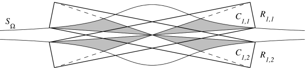
Figure 1: Part of a stratified starlike cover of $S_{\Omega}$: the shaded region, $S_{1}$, is covered by rectangles $R_{1,1}$ and $R_{1,2}$. See remark 1.6.

For any set $E\subset{\mathbb{R}^{n}}$ the collection ${\mathcal{B}}(E)$ consists of all translates and (isotropic) dilates of $E$.

Theorem 1.7.

Suppose $\Omega\in{L\log L({\mathbb{S}^{n-1}})}$ is positively homogeneous of degree $0$ and $\int_{\mathbb{S}^{n-1}}\Omega(\theta)\,d\theta=0$. Let $\{R_{m,k}\colon m\geq 0,1\leq k<k_{m}\}$ be a stratified starlike cover of the set $S=S_{\Omega}$. Assume $1<p<\infty$ and that $w$ is a non-negative measurable function that satisfies the following condition: there exists $r>1$ such that for all $m\geq 0$, $1\leq k<k_{m}$ there is a constant $K_{m,k}>0$ so that

$$\biggl{(}{\frac{1}{\lvert R\rvert}\int_{R}w}\biggr{)}^{1/p}\biggl{(}{\frac{1}{\lvert R\rvert}\int_{R}w^{-rp^{\prime}/p}}\biggr{)}^{1/rp^{\prime}} \leq\frac{K_{m,k}}{\lvert R_{m,k}\rvert}, 1<p\leq 2$$ if , (1.4a)

$$\biggl{(}{\frac{1}{\lvert R\rvert}\int_{R}w^{r}}\biggr{)}^{1/rp}\biggl{(}{\frac{1}{\lvert R\rvert}\int_{R}w^{-p^{\prime}/p}}\biggr{)}^{1/p^{\prime}} \leq\frac{K_{m,k}}{\lvert R_{m,k}\rvert}, 2\leq p<\infty$$ if , (1.4b)

holds for all $R\in{\mathcal{B}}(R_{m,k})$ and the constants $K_{m,k}$ satisfy

$$\sum_{m=0}^{\infty}\sum_{k=1}^{k_{m}-1}(m+1)K_{m,k}<\infty.$$ (1.5)

Then there exists $\sigma>1$ such that if $h\in{\mathcal{H}}(\sigma)$ the operators $T_{\epsilon}$, $\epsilon>0$, can be extended to a uniformly bounded family of operators on ${L^{p}_{w}}$ and the operator $T$ can be extended to a bounded operator on ${L^{p}_{w}}$.

Theorem 1.5 of [12] is the corresponding result when $h\equiv 1$. It is included as a special case of the above theorem. More generally, if $h\in{L^{\infty}}({\mathbb{R}^{+}})$ then clearly $h\in{\mathcal{H}}(\sigma)$ for all $\sigma>1$. Hence, in this case, whether $T$ is bounded does not depend on the properties of $h$.

Remark 1.8.

Condition 1.4 implies $w\in A_{p}$: Since (1.4) holds for all translates and dilates of any of the fixed rectangles $R_{m,k}$, it holds for all cubes in place of the rectangles. Then Hölder’s inequality shows $w\in A_{p}$.

Corollary 1.9.

Suppose $\Omega$ and the sets $\{R_{m,k}\}$ are as in Theorem 1.7, and that instead of (1.4) there exists a constant $K>0$ such that for all $m\geq 0$, $1\leq k<k_{m}$ and $R\in{\mathcal{B}}(R_{m,k})$

$$\biggl{(}{\frac{1}{\lvert R\rvert}\int_{R}w}\biggr{)}^{1/p}\biggl{(}{\frac{1}{\lvert R\rvert}\int_{R}w^{-p^{\prime}/p}}\biggr{)}^{1/p^{\prime}}\leq K.$$ (1.6)

Then there exists $\sigma>1$ such that if $h\in{\mathcal{H}}(\sigma)$ then $T$ can be extended to a bounded operator on ${L^{p}_{w}}$ and the truncated operators $T_{\epsilon}$, $\epsilon>0$, can be extended to a uniformly bounded family of operators on ${L^{p}_{w}}$.

Proof.

Since (1.6) is uniform in $m$ and $k$ the reverse Hölder’s inequality applied to $w$ and $w^{-p^{\prime}/p}$ shows that $w$ satisfies condition (1.4) with $K_{m,k}=K\lvert R_{m,k}\rvert$ and for some $r>1$, see [12]. Then (1.5) is a consequence of the hypothesis $\Omega\in{L\log L({\mathbb{S}^{n-1}})}$ and of $\sum_{k}\lvert R_{m,k}\rvert\leq c\lvert S_{m}\rvert$, see (4.10). ∎

Theorem 1.10.

Suppose $\Omega$ and the sets $\{R_{m,k}\}$ are as in Theorem 1.7, $h\in{L^{\infty}}({\mathbb{R}^{+}})$, and for all $m\geq 0$, $1\leq k<k_{m}$ there exists a constant $K_{m,k}>0$ such that for all $R\in{\mathcal{B}}(R_{m,k})$

$$\biggl{(}{\frac{1}{\lvert R\rvert}\int_{R}w}\biggr{)}^{1/2}\biggl{(}{\frac{1}{\lvert R\rvert}\int_{R}w^{-1}}\biggr{)}^{1/2}\leq\frac{K_{m,k}}{\lvert R_{m,k}\rvert},$$ (1.7)

and the constants $K_{m,k}$ satisfy (1.5). Then $T$ can be extended to a bounded operator on $L^{2}_{w}$, and the truncated operators $T_{\epsilon}$, $\epsilon>0$, can be extended to a uniformly bounded family of operators on $L^{2}_{w}$.

2 Maximal operators

We define the maximal operator

$$M_{H}f(x)=\sup_{r>0}\frac{1}{r^{n}}\int_{\lvert y\rvert<r}{H(x,y)\lvert f(x-y)\rvert\,dy},$$ (2.1)

where the non-negative function $H$ satisfies for some $\sigma>1$ and $C_{H}>0$

$$\int_{\lvert y\rvert<r}{H(x,y)^{\sigma}\,dy}\leq C_{H}r^{n}$$ (2.2)

for all $x\in{\mathbb{R}^{n}}$ and $r>0$.

There are two simple examples of functions that satisfy (2.2). One is given by radial functions in the class ${\mathcal{H}}(\sigma)$, i.e., $H(x,y)=\lvert h_{x}(\lvert y\rvert)\rvert$ and $h_{x}\in{\mathcal{H}}(\sigma)$ uniformly in $x\in{\mathbb{R}^{n}}$. Another example is given by homogeneous functions: let $H(x,y)=\lvert\Phi_{x}(y)\rvert$, where $\Phi_{x}$ is homogeneous of degree zero and $\Phi_{x}\in L^{\sigma}({\mathbb{S}^{n-1}})$ uniformly in $x\in{\mathbb{R}^{n}}$. In both cases the verification of (2.2) follows by writing the integral in (2.2) in polar coordinates (see also Lemma 4.4 below).

In this section the letter $C$ denotes a constant that depends on $H$ only through the constant $C_{H}$ in equation (2.2) above.

2.1 Weighted norm inequalities

In order to study the starlike maximal function $M_{S,H}$ (see Theorem 2.4 below) we need to know precisely how the operator norm of $M_{H}$ on ${L^{p}_{w}}$ depends on the weight.

Theorem 2.1.

Let $1<p<\infty$ and assume that the weight $w$ satisfies for some $r>1$

$$\left({\frac{1}{\lvert Q\rvert}\int_{Q}w}\right)^{1/p}\left({\frac{1}{\lvert Q\rvert}\int_{Q}w^{-rp^{\prime}/p}}\right)^{1/rp^{\prime}}\leq K$$ (2.3)

for all cubes $Q\subset{\mathbb{R}^{n}}$. If $H$ satisfies (2.2) for some $\sigma>r^{\prime}p^{\prime}$ then $M_{H}$ is bounded on ${L^{p}_{w}}$ with operator norm bounded by $CK$.

Theorem 2.1 follows easily from the next result, which is a special case of Theorem 2.11 in [8]. The Hardy-Littlewood maximal operator is defined by $Mf(x)=\sup_{r>0}r^{-n}\int_{\lvert y\rvert<r}{\lvert f(x-y)\rvert\,dy}$.

Theorem 2.2 (Pérez).

Let $1<p<\infty$ and suppose $w$ satisfies (2.3) for some $r>1$. Then ${\lVert Mf\rVert_{p,w}}\leq CK{\lVert f\rVert_{p,w}}$, where $C$ is independent of $f$ and $K$.

The estimate $CK$ for the operator norm is not stated in [8], but it is easy to see that it follows from the proof given there.

Proof of Theorem 2.1.

By Hölder’s inequality we have

$$M_{H}f(x)\leq\sup_{r>0}\left(\frac{1}{r^{n}}\int_{\lvert y\rvert<r}{H(x,y)^{\sigma}\,dy}\right)^{1/\sigma}\left(\frac{1}{r^{n}}\int_{\lvert y\rvert<r}{\lvert f(x-y)\rvert^{\sigma^{\prime}}\,dy}\right)^{1/\sigma^{\prime}}.$$

Since $h$ satisfies (2.2) we get $M_{H}f(x)\leq C_{H}^{1/\sigma}\bigl{[}M(\lvert f\rvert^{\sigma^{\prime}})(x)\bigr{]}^{1/\sigma^{\prime}}$, where $M$ is the Hardy-Littlewood maximal function. Therefore ${\lVert M_{H}f\rVert_{p,w}}\leq C{\bigl{\lVert}M(\lvert f\rvert^{\sigma^{\prime}})\bigr{\rVert}_{p_{1},w}^{1/{\sigma^{\prime}}}}$, where $p_{1}=p/\sigma^{\prime}$.

Condition (2.3) implies a similar condition with the power $p_{1}$ in place of $p$: generalizing an idea from [9] we claim that there exists $\rho>1$ such that

$$\left({\frac{1}{\lvert Q\rvert}\int_{Q}w}\right)^{1/p_{1}}\left({\frac{1}{\lvert Q\rvert}\int_{Q}w^{-\rho p_{1}^{\prime}/p_{1}}}\right)^{1/\rho p_{1}^{\prime}}\leq K^{\sigma^{\prime}}$$ (2.4)

for all cubes $Q\subset{\mathbb{R}^{n}}$. To prove this claim note that the equation $rp^{\prime}/p=\rho p_{1}^{\prime}/p_{1}$ is equivalent with $\rho=r(p_{1}-1)/(p-1)$. It is easy to see that $\rho>1$ is equivalent with $\sigma>r^{\prime}p^{\prime}$. Raising both sides of (2.3) to the power $\sigma^{\prime}$ gives (2.4). Now Theorem 2.2 applied on $L^{p_{1}}_{w}$ gives ${\lVert M_{H}f\rVert_{p,w}}\leq C\bigl{(}K^{\sigma^{\prime}}{\bigl{\lVert}\lvert f\rvert^{\sigma^{\prime}}\bigr{\rVert}_{p_{1},w}}\bigr{)}^{1/\sigma^{\prime}}=CK{\lVert f\rVert_{p,w}}.$ ∎

Corollary 2.3.

Let $1<p<\infty$ and $w\in A_{p}$. Then there exists $\sigma>1$ such that if $H$ satisfies (2.2) then $M_{H}$ is bounded on ${L^{p}_{w}}$.

Proof.

The reverse Hölder’s inequality implies $w$ satisfies (2.3) for some $r>1$, see [3, 7]. ∎

2.2 A starlike maximal operator

If $S\subset{\mathbb{R}^{n}}$ is an arbitrary measurable star-shaped set centered at the origin, a collection $\{R_{j}\}$ of rectangles is a starlike cover of $S$ if each $R_{j}$ is a rectangle centered at the origin, $S\subset\bigcup_{j}R_{j}$ up to a set of measure zero, and $\sum_{j}\lvert R_{j}\rvert\leq c_{n}\lvert S\rvert$, where $c_{n}$ depends only on the dimension of ${\mathbb{R}^{n}}$. It is shown in [2] that such a cover always exists (see also remark 1.6).

Theorem 2.4.

Assume $H$ is a non-negative measurable function on ${\mathbb{R}^{n}}\times{\mathbb{R}^{n}}$, $S\subset{\mathbb{R}^{n}}$ is star-shaped about the origin, and $\{R_{j}\}$ is a starlike cover of $S$. Define the starlike maximal operator

$$M_{S,H}f(x)=\sup_{t>0}\frac{1}{t^{n}}\int_{tS}H(x,y)\lvert f(x-y)\rvert\,dy.$$ (2.5)

Let $1<p<\infty$ and suppose the weight $w$ satisfies for some $r>1$

$$\left({\frac{1}{\lvert R\rvert}\int_{R}w}\right)^{1/p}\left({\frac{1}{\lvert R\rvert}\int_{R}w^{-rp^{\prime}/p}}\right)^{1/rp^{\prime}}\leq\frac{K_{j}}{\lvert R_{j}\rvert},$$ (2.6)

for all $R\in{\mathcal{B}}(R_{j})$, where the constants $K_{j}$ satisfy $\sum_{j}K_{j}<\infty$. If $H$ satisfies

$$\int_{tR_{j}}H(x,y)^{\sigma}\,dy\leq C\lvert tR_{j}\rvert,\quad x\in{\mathbb{R}^{n}},$$ (2.7)

for all $t>0$ and all $j$, and for some $\sigma>r^{\prime}p^{\prime}$, then $M_{S,H}$ is bounded on ${L^{p}_{w}}$ with operator norm bounded by $C\sum_{j}K_{j}$, where $C$ is independent of $\{K_{j}\}$.

Remark 2.5.

Theorem 2.4 generalizes to a fractional version of the operator $M_{S,H}$ defined by

$$M_{\mu,S,H}f(x)=\sup_{t>0}\frac{1}{t^{n-\mu}}\int_{tS}H(x,y)\lvert f(x-y)\rvert\,dy,\quad 0\leq\mu<n.$$

The result proved in [8], Theorem 2.11, is much more general than Theorem 2.2 stated above. Theorem 2.11 gives conditions when the fractional maximal operator is bounded from $L^{p}_{w}$ to $L^{q}_{v}$, $1<p\leq q<\infty$. The same proof that is given above for Theorem 2.1 combined with the full strength of Theorem 2.11 of [8] can be easily used to get two weight norm estimates for another fractional maximal operator,

$$M_{\mu,H}f(x)=\sup_{r>0}\frac{1}{r^{n-\mu}}\int_{\lvert y\rvert<r}H(x,y)\lvert f(x-y)\rvert\,dy,\quad 0\leq\mu<n,$$

from $L^{p}_{w}$ to $L^{q}_{v}$, when the weights $v$ and $w$ satisfy the same conditions as in [8], and $\sigma>\max\{r^{\prime}p^{\prime},n/(n-\mu)\}$. Using these results Theorem 2.4 generalizes to $M_{\mu,S,H}$ when the weights $v$ and $w$ satisfy the conditions of Theorem 5(C) of [2] and $\sigma$ is as above.

Remark 2.6.

It is shown below in Lemma 4.4 that if $H(x,y)=h_{x}(\lvert y\rvert)$ and $h_{x}\in{\mathcal{H}}(\sigma)$ uniformly in $x\in{\mathbb{R}^{n}}$, then $H$ satisfies (2.7). For homogeneous functions the situation is more complicated:

An interesting special case is $H(x,y)=\lvert\Omega(y)\rvert$, $\Omega$ is homogeneous of degree zero, and the set $S=S_{\Omega}$ is the star-shaped set associated with $\Omega$ as in definition 1.1. If the cover $\{R_{j}\}$ is constructed as in remark 1.6 (i.e., the rectangles $\{R_{j}\}$ are the the same as $\{R_{m,k}\}$ after a renumbering of the latter), condition (2.7) implies $\Omega\in{L^{\infty}}({\mathbb{S}^{n-1}})$, as we now show.

Using the notation of remark 1.6 let $D_{m,k}$ be the intersection of a certain cone inside $R_{m,k}$ with ${\mathbb{S}^{n-1}}$. These disks were chosen to cover the set $\Theta_{m}$. But then there exists a constant $\beta\in(0,1)$ such that for each $m$ at least one of the disks covering $\Theta_{m}$, say $D_{m,k_{m}}$, has the property that $\rho(\theta)>2^{m-1}$ on a subset of $D_{m,k_{m}}$ with surface measure at least $\beta\lvert D_{m,k_{m}}\rvert$ (we use $\lvert\cdot\rvert$ also for surface measure). Then, using $\lvert R_{m,k_{m}}\rvert\approx 2^{nm}\lvert D_{m,k_{m}}\rvert$, we have

$${\frac{1}{\lvert R_{m,k_{m}}\rvert}\int_{R_{m,k_{m}}}\lvert\Omega(y)\rvert\,dy}\geq{c_{n}}{\frac{1}{\lvert D_{m,k_{m}}\rvert}\int_{D_{m,k_{m}}}\lvert\Omega(\theta)\rvert\,d\theta}.$$

The right hand side is larger than $c_{n,\beta}2^{n(m-1)}$, which shows (2.7) is impossible when the set $S_{\Omega}$ is essentially unbounded. Hence $\Omega\in{L^{\infty}}({\mathbb{S}^{n-1}})$.

If the covering is less efficient there are examples of unbounded $\Omega$ that satisfy (2.7) and yield a bounded operator $M_{S_{\Omega},\Omega}$. In two dimensions let

$$\Omega(\theta)=\sum_{k=1}^{\infty}2^{2k}{\chi\vphantom{\big{|}}}_{I_{k}}(\theta),\quad\text{where $I_{k}=[2^{-3k}-2^{-5k},2^{-3k}]$,}$$

and $R_{j}=[-2^{j},2^{j}]\times[-2^{-2j},2^{-2j}]$, so that $\sum_{j}\lvert R_{j}\rvert<\infty$ and $\bigcup_{j}R_{j}\supset S_{\Omega}$. A straightforward computation shows $\Omega$ satisfies (2.7). Examples of weights that satisfy (2.6) are $w(x)=\lvert x\rvert^{\alpha}$ for $-1<\alpha<p$. As a result $M_{S_{\Omega},\Omega}$ is bounded on ${L^{p}_{w}}$.

It is of course easy to find examples of star-shaped sets $S$ and unrelated homogeneous functions $H(x,y)=\lvert\Phi_{x}(y)\rvert$, $\Phi(y)\in L^{\sigma}({\mathbb{S}^{n-1}})$, that satisfy (2.7): one idea is simply to require $\Phi$ to be (uniformly) bounded along any unbounded arms of $S$.

Proof of Theorem 2.4.

The proof is almost identical with the one given in [2] in the case $H\equiv 1$, but since there are many differences in the details we present the full argument:

Since the sets $R_{j}$ cover $S$ we have ${\chi\vphantom{\big{|}}}_{S}\leq\sum_{j}{\chi\vphantom{\big{|}}}_{R_{j}}$, hence $M_{S,H}f\leq\sum_{j}M_{R_{j},H}f$. Let $\Lambda_{j}\colon{\mathbb{R}^{n}}\rightarrow{\mathbb{R}^{n}}$ be an invertible linear transformation such that $R_{j}=\Lambda_{j}Q_{1}$, where $Q_{1}$ is the unit cube centered at the origin. A change of coordinates gives

$$\int_{R_{j}}H(x,y)f(x-y)\,dy=\lvert\det\Lambda_{j}\rvert\int_{Q_{1}}H(x,\Lambda_{j}y)f(\Lambda_{j}(\Lambda_{j}^{-1}x-y))\,dy,$$

and letting $\Lambda_{j}f(x)=\lvert\det\Lambda_{j}\rvert f(\Lambda_{j}x)$, $H_{j}(x,y)=H(x,\Lambda_{j}y)$, we have

$$M_{R_{j},H}f(x)\leq C\lvert\det\Lambda_{j}\rvert(\Lambda_{j}^{-1}M_{H_{j}}\Lambda_{j}f)(x).$$

Using ${\lVert\Lambda_{j}^{-1}g\rVert_{p,w}}=\lvert\det\Lambda_{j}\rvert^{-1}{\lVert g\rVert_{p,\Lambda_{j}w}}$ we get

$${\lVert M_{R_{j},H}f\rVert_{p,w}} \leq C\lvert\det\Lambda_{j}\rvert\,{\lVert\Lambda_{j}^{-1}M_{H_{j}}\Lambda_{j}f\rVert_{p,w}}=C{\lVert M_{H_{j}}\Lambda_{j}f\rVert_{p,\Lambda_{j}w}}$$

$$\leq C{\lVert M_{H_{j}}\rVert_{L^{p}_{\Lambda_{j}w},L^{p}_{\Lambda_{j}w}}}{\lVert\Lambda_{j}f\rVert_{p,\Lambda_{j}w}}$$

$$=C\lvert\det\Lambda_{j}\rvert\,{\lVert M_{H_{j}}\rVert_{L^{p}_{\Lambda_{j}w},L^{p}_{\Lambda_{j}w}}}{\lVert f\rVert_{p,w}}.$$

Thus ${\lVert M_{S,H}f\rVert_{p,w}}\leq C{\lVert f\rVert_{p,w}}\sum_{j}\lvert R_{j}\rvert\,{\lVert M_{H_{j}}\rVert_{L^{p}_{\Lambda_{j}w},L^{p}_{\Lambda_{j}w}}}$, since $\lvert R_{j}\rvert=\lvert\det\Lambda_{j}\rvert$.

The functions $H_{j}$ satisfy condition (2.2) uniformly in $j$: Since for any $r>0$ there is $t>0$ such that $tR_{j}\subset\Lambda_{j}B(0,r)\subset 2tR_{j}$, we get from (2.7) that

$$\int_{\lvert y\rvert<r}H_{j}(x,y)^{\sigma}\,dy =\lvert\det\Lambda_{j}\rvert^{-1}\int_{\Lambda_{j}B(0,r)}H(x,y)^{\sigma}\,dy$$

$$\leq C_{H}\lvert\det\Lambda_{j}\rvert^{-1}\lvert\Lambda_{j}B(0,r)\rvert,$$

which is equal to $Cr^{n}$. By a similar change of coordinates condition (2.6) is equivalent with

$$\left({\frac{1}{\lvert Q\rvert}\int_{Q}\Lambda_{j}w}\right)^{1/p}\left({\frac{1}{\lvert Q\rvert}\int_{Q}(\Lambda_{j}w)^{-rp^{\prime}/p}}\right)^{1/rp^{\prime}}\leq\frac{K_{j}}{\lvert R_{j}\rvert},$$

for all cubes $Q\subset{\mathbb{R}^{n}}$. By Theorem 2.1, ${\lVert M_{H_{j}}\rVert_{L^{p}_{\Lambda_{j}w},L^{p}_{\Lambda_{j}w}}}\leq CK_{j}/\lvert R_{j}\rvert$. Therefore ${\lVert M_{S,H}f\rVert_{p,w}}\leq\bigr{(}C\sum_{j}K_{j}\bigl{)}{\lVert f\rVert_{p,w}}$. ∎

2.3 Vector-valued inequalities

In this section we prove a generalization of the weighted vector-valued inequality for the maximal function:

Theorem 2.7 (Andersen and John [1]).

Let $1<p,q<\infty$ and suppose $w\in A_{p}$. There is a constant $C_{p,q,w}$ such that

$$\Bigl{\lVert}\Bigl{(}\sum_{j}\lvert Mf_{j}\rvert^{q}\Bigr{)}^{1/q}\Bigr{\rVert}_{p,w}\leq C_{p,q,w}\Bigl{\lVert}\Bigl{(}\sum_{j}\lvert f_{j}\rvert^{q}\Bigr{)}^{1/q}\Bigr{\rVert}_{p,w},$$

where $C_{p,q,w}$ depends on $w$ only through its $A_{p}$ constant.

The corresponding result for the operator $M_{H}$ is as follows:

Theorem 2.8.

Let $1<p,q<\infty$ and $w\in A_{p}$. There exists $\sigma>1$ such that if $H$ satisfies (2.2) the vector-valued inequality

$$\Bigl{\lVert}\Bigl{(}\sum_{j}\lvert M_{H}f_{j}\rvert^{q}\Bigr{)}^{1/q}\Bigr{\rVert}_{p,w}\leq C\Bigl{\lVert}\Bigl{(}\sum_{j}\lvert f_{j}\rvert^{q}\Bigr{)}^{1/q}\Bigr{\rVert}_{p,w}$$ (2.8)

holds for any sequence $\{f_{j}\}$.

Proof.

By Hölder’s inequality we have

$$\Bigl{\lVert}\Bigl{(}\sum_{j}\lvert M_{H}f_{j}\rvert^{q}\Bigr{)}^{1/q}\Bigr{\rVert}_{p,w}\leq C_{H}^{1/\sigma}\Bigl{\lVert}\Bigl{(}\sum_{j}[M(\lvert f_{j}\rvert^{\sigma^{\prime}})]^{q/\sigma^{\prime}}\Bigr{)}^{1/q}\Bigr{\rVert}_{p,w}$$

and by Theorem 2.7 this is bounded by $C\bigl{\lVert}\bigl{(}\sum_{j}\lvert f_{j}\rvert^{q}\bigr{)}^{1/q}\bigr{\rVert}_{p,w}$, provided that $q/\sigma^{\prime}>1$ and $w\in A_{p/\sigma^{\prime}}$, both of which hold when $\sigma$ is large enough (see [3, 7]). ∎

3 Proof of the representation formula

Recall the class of functions ${\mathcal{H}}(\sigma)$ from definition 1.2.

Lemma 3.1.

Let $1\leq\sigma<\infty$, $h\in{\mathcal{H}}(\sigma)$, and $C_{h}$ be as in the definition of ${\mathcal{H}}(\sigma)$. If $0<a<b<\infty$, then $\int_{a}^{b}\lvert h(r)\rvert^{\sigma}\,dr/r\leq C_{h}\lceil\log_{2}b/a\rceil$, where $\lceil x\rceil$ is the ceiling of $x\in\mathbb{R}$, i.e., the smallest integer greater than or equal to $x$.

Proof.

Let $N=\lceil\log_{2}b/a\rceil$, then

$$\int_{a}^{b}\lvert h(r)\rvert^{\sigma}\,\frac{dr}{r}\leq\sum_{k=0}^{N-1}\int_{2^{k}a}^{2^{k+1}a}\lvert h(r)\rvert^{\sigma}\,\frac{dr}{r}\leq C_{h}N.\qed$$

Lemma 3.2.

Let $\Omega\in L^{1}({\mathbb{S}^{n-1}})$ be positively homogeneous of degree $0$. Then for all $y\in{\mathbb{R}^{n}}$

$$\int_{0}^{\infty}\frac{1}{t^{n}}{\chi\vphantom{\big{|}}}_{tS\setminus B(0,\epsilon)}(y)\frac{dt}{t}=\frac{1}{n}{\chi\vphantom{\big{|}}}_{B(0,\epsilon)^{c}}(y)\frac{\lvert\Omega(y)\rvert}{\lvert y\rvert^{n}}$$ (3.1)

in the sense that either both sides are finite and equal or they are both infinite.

Proof.

The identity follows from the fact that $y\in tS$ if and only if $\lvert y\rvert<t\lvert\Omega(y)\rvert^{1/n}$. ∎

Proof of Theorem 1.3.

Fix $x\in{\mathbb{R}^{n}}$ and $\epsilon>0$. By Lemma 3.2 the operator $T_{\epsilon}$ can be written as

$$T_{\epsilon}f(x)=n\int_{\mathbb{R}^{n}}\int_{0}^{\infty}\frac{1}{t^{n}}{\chi\vphantom{\big{|}}}_{tS\setminus B(0,\epsilon)}(y)\frac{dt}{t}\operatorname{sgn}\Omega(y)h(\lvert y\rvert)f(x-y)\,dy.$$ (3.2)

Changing the order of integration—justification is given below—we obtain

$$T_{\epsilon}f(x)=n\int_{0}^{\infty}\frac{1}{t^{n}}\int_{tS\setminus B(0,\epsilon)}\operatorname{sgn}\Omega(y)h(\lvert y\rvert)f(x-y)\,dy\,\frac{dt}{t},$$

as was to be shown.

To justify the change in the order of integration we need to show that

$$n\int_{{\mathbb{R}^{n}}}\int_{0}^{\infty}\frac{1}{t^{n}}{\chi\vphantom{\big{|}}}_{tS\setminus B(0,\epsilon)}(y)\frac{dt}{t}\lvert h(\lvert y\rvert)f(x-y)\rvert\,dy\\ =\int_{\lvert y\rvert>\epsilon}\frac{\lvert\Omega(y)\rvert}{\lvert y\rvert^{n}}\lvert h(\lvert y\rvert)f(x-y)\rvert\,dy$$ (3.3)

is finite. A change into polar coordinates $y=r\theta$ with $r=\lvert y\rvert$ and $\theta=y/\lvert y\rvert\in{\mathbb{S}^{n-1}}$ shows the right-hand side of (3.3) is

$$\int_{\mathbb{S}^{n-1}}\lvert\Omega(\theta)\rvert\int_{\epsilon}^{\infty}\frac{\lvert h(r)\rvert}{r}\lvert f(x-r\theta)\rvert\,dr\,d\theta,$$ (3.4)

where we used $d\theta$ for the surface measure on ${\mathbb{S}^{n-1}}$. We estimate (3.4) by

$${\lVert f\rVert_{\infty}}\int_{\mathbb{S}^{n-1}}\lvert\Omega(\theta)\rvert\,d\theta\int_{\epsilon}^{R+\lvert x\rvert}\lvert h(r)\rvert\,\frac{dr}{r},$$

where $R$ is such that $\operatorname{supp}f\subset B(0,R)$. By Lemma 3.1 the second integral is finite for all $x\in{\mathbb{R}^{n}}$, thus also (3.3) is finite everywhere.

Since the case $f\in L^{p}({\mathbb{R}^{n}})$, $1<p<\infty$, is not used in the rest of the paper, we only sketch its proof: We let $Q\subset{\mathbb{R}^{n}}$ be an arbitrary cube and compute the $L^{p}(Q)$ norm of (3.4). Using Minkowski’s inequality, $h\in{\mathcal{H}}(p^{\prime})$, and $f\in L^{p}({\mathbb{R}^{n}})$, we can estimate (3.4) by $C(Q,h,\epsilon,f)\int_{\mathbb{S}^{n-1}}\lvert\Omega(\theta)\rvert\,d\theta<\infty$. Since the cube $Q$ is arbitrary, this shows that (3.3) is finite almost everywhere. ∎

4 Preliminaries

4.1 Weighted Littlewood-Paley theory

For proofs of the following facts see [6] and [12].

Let $\Psi\in C_{0}^{\infty}((\frac{1}{2},2))$ be such that $\Psi\geq 0$ and $\sum_{j\in\mathbb{Z}}\Psi^{2}(2^{j}t)=1$ for $t>0$. Let $\widehat{\psi}(\xi)=\Psi(\lvert\xi\rvert)$ and define $Q_{j}f=\psi_{j}*f$, where $\psi_{j}(x)=2^{-nj}\psi(2^{-j}x)$.

Let $1<p<\infty$ and $w\in A_{p}$. Then there exists $C_{p,w}>0$ such that the following estimates hold:

$$C_{p,w}^{-1}{\lVert f\rVert_{p,w}}\leq\biggl{\lVert}\biggl{(}\sum_{j}\lvert Q_{j}f\rvert^{2}\biggr{)}^{1/2}\biggr{\rVert}_{p,w}\leq C_{p,w}{\lVert f\rVert_{p,w}},$$ (4.1)

$$C_{p,w}^{-1}{\lVert f\rVert_{p,w}}\leq\biggl{\lVert}\biggl{(}\sum_{j}\lvert Q_{j}^{2}f\rvert^{2}\biggr{)}^{1/2}\biggr{\rVert}_{p,w}\leq C_{p,w}{\lVert f\rVert_{p,w}},$$ (4.2)

$${\Bigl{\lVert}\sum_{j}Q_{j}f_{j}\Bigr{\rVert}_{p,w}}\leq C_{p,w}\biggl{\lVert}\biggl{(}\sum_{j}\lvert Q_{j}f_{j}\rvert^{2}\biggr{)}^{1/2}\biggr{\rVert}_{p,w},$$ (4.3)

$${\Bigl{\lVert}\sum_{j}Q_{j}^{2}f_{j}\Bigr{\rVert}_{p,w}}\leq C_{p,w}\biggl{\lVert}\biggl{(}\sum_{j}\lvert Q_{j}^{2}f_{j}\rvert^{2}\biggr{)}^{1/2}\biggr{\rVert}_{p,w}.$$ (4.4)

The identity $\sum_{j}Q_{j}^{2}=\text{Id}$ holds in many senses, e.g., for smooth functions $f\in L^{2}$

$$\lim\limits_{k,l\rightarrow\infty}\sum_{j=-k}^{l}Q_{j}^{2}f(x)=f(x)$$ (4.5)

for all $x\in{\mathbb{R}^{n}}$.

4.2 Lemmata on homogeneous and radial functions

In the following lemmata $\Omega$ is always positively homogeneous of degree $0$ and $S=S_{\Omega}$ is the star-shaped set associated with $\Omega$ as in definition 1.1.

Lemma 4.1.

The following equalities and estimates hold:

$$\lvert S\rvert=\int_{S}\,dy =\frac{1}{n}\int_{\mathbb{S}^{n-1}}\lvert\Omega(\theta)\rvert\,d\theta,$$ (4.6)

$$\int_{S}\operatorname{sgn}\Omega(y)\,dy =\frac{1}{n}\int_{\mathbb{S}^{n-1}}\Omega(\theta)\,d\theta,$$ (4.7)

$$\int_{S}\operatorname{log^{+}}\lvert y\rvert\,dy \leq\frac{1}{n^{2}}{\lVert\Omega\rVert_{{L\log L}}},$$ (4.8)

$$\int_{S}\bigl{|}\log\lvert y\rvert\bigr{|}\,dy \leq\frac{1}{n^{2}}({\lVert\Omega\rVert_{{L\log L}}}+1),$$ (4.9)

$$\sum_{m=0}^{\infty}(m+1)\lvert S_{m}\rvert \leq c_{n}{\lVert\Omega\rVert_{{L\log L}}},$$ (4.10)

for some constant $c_{n}$ depending only on the dimension $n$.

Proof.

Using polar coordinates $y=r\theta$ with $r>0$, $\theta\in{\mathbb{S}^{n-1}}$, and recalling that $\rho(\theta)=\lvert\Omega(\theta)\rvert^{1/n}$, we have

$$\int_{S}\,dy=\int_{\mathbb{S}^{n-1}}\int_{0}^{\rho(\theta)}r^{n-1}\,dr\,d\theta=\frac{1}{n}\int_{\mathbb{S}^{n-1}}\lvert\Omega(\theta)\rvert\,d\theta.$$

This proves (4.6). The proofs of (4.7) through (4.9) are similar.

To prove estimate (4.10) recall the sets $\Theta_{m}$ from (1.3) and notice that $\lvert S_{m}\rvert=\frac{1}{n}\int_{\Theta_{m}}\lvert\Omega(\theta)\rvert\,d\theta$ by (4.6). This gives

$$\sum_{m=0}^{\infty}(m+1)\lvert S_{m}\rvert=\frac{1}{n}\int_{\Theta_{0}}\lvert\Omega(\theta)\rvert\,d\theta+\frac{1}{n}\sum_{m=1}^{\infty}\int_{\Theta_{m}}(m+1)\lvert\Omega(\theta)\rvert\,d\theta.$$

When $m\geq 1$, $\rho(\theta)>2^{m-1}\geq 1$ on $\Theta_{m}$; thus $m<1+\operatorname{log^{+}_{2}}\lvert\Omega(\theta)\rvert^{1/n}$ and so

$$\sum_{m=0}^{\infty}(m+1)\lvert S_{m}\rvert\leq\frac{1}{n}\int_{\mathbb{S}^{n-1}}\lvert\Omega(\theta)\rvert\,d\theta+\frac{1}{n}\int_{\mathbb{S}^{n-1}}\lvert\Omega(\theta)\rvert(2+\operatorname{log^{+}_{2}}\lvert\Omega(\theta)\rvert^{1/n})\,d\theta,$$

which is bounded by $c_{n}{\lVert\Omega\rVert_{{L\log L}}}$. ∎

We will use the following characterizations of the class ${\mathcal{H}}(\sigma)$ interchangeably:

Lemma 4.2.

For fixed $1\leq\sigma<\infty$ the following are equivalent:

1. there exists $C>0$ such that $\int_{R}^{2R}\lvert h(r)\rvert^{\sigma}\,dr\leq CR$ for all $R>0$.

2. there exists $C>0$ such that $\int_{0}^{R}\lvert h(r)\rvert^{\sigma}\,dr\leq CR$ for all $R>0$.

3. there exists $C>0$ such that $\int_{R}^{2R}\lvert h(r)\rvert^{\sigma}\,\frac{dr}{r}\leq C$ for all $R>0$.

The only non-trivial implication is from (a) to (b), which follows by writing the integral over $[0,R]$ as the sum of integrals over $[2^{-k-1}R,2^{-k}R]$, $0\leq k<\infty$.

Lemma 4.3.

Suppose that $h\in{\mathcal{H}}(1)$ vanishes in a neighborhood of the origin. Then there are constants $C_{1}(h)>0$ and $C_{2}(h)>0$ such that

$$\int_{0}^{R}\lvert h(r)\rvert\frac{dr}{r}\leq C_{1}(h)+C_{2}(h)\operatorname{log^{+}}R,$$ (4.11)

and a constant $C(h,n)>0$ such that

$$\int_{0}^{1}\int_{S}\lvert h(t\lvert y\rvert)\rvert\,dy\frac{dt}{t}\leq C(h,n){\lVert\Omega\rVert_{{L\log L}}}.$$ (4.12)

Sketch of Proof.

The first part of the lemma follows immediately from Lemma 3.1. For the second part change the order of integration in (4.12), change variables in the $t$-integral, and use (4.11), (4.6), and (4.8) ∎

Lemma 4.4.

Let $1\leq\sigma<\infty$, $h\in{\mathcal{H}}(\sigma)$, and $E\subset{\mathbb{R}^{n}}$ be any measurable set star-shaped about the origin. Then

$$\int_{E}\lvert h(t\lvert y\rvert)\rvert^{\sigma}\,dy\leq c_{n}C_{h}\lvert E\rvert,\quad\text{for any $t>0$,}$$

where $C_{h}$ is as in the definition of $h\in{\mathcal{H}}(\sigma)$ (definition 1.2).

Proof.

In polar coordinates

$$\int_{E}\lvert h(t\lvert y\rvert)\rvert^{\sigma}\,dy=\int_{\mathbb{S}^{n-1}}\int_{0}^{\rho(\theta)}\lvert h(tr)\rvert^{\sigma}r^{n-1}\,dr\,d\theta,$$

where $\rho(\theta)$ is the boundary function of $E$, that is, up to a set of measure zero $E$ is given by $\{x\in{\mathbb{R}^{n}}\colon\lvert x\rvert\leq\rho(x)\}$. Now the $r$-integral equals

$$\sum_{k=0}^{\infty}\int_{2^{-k-1}\rho(\theta)}^{2^{-k}\rho(\theta)}\lvert h(tr)\rvert^{\sigma}r^{n-1}\,dr\leq\sum_{k=0}^{\infty}2^{n(-k-1)}\rho(\theta)^{n}\int_{2^{-k-1}\rho(\theta)}^{2^{-k}\rho(\theta)}\lvert h(tr)\rvert^{\sigma}\,\frac{dr}{r}.$$

Lemma 4.2 and a change of coordinates show that the last integral is bounded by a constant, thus $\int_{0}^{\rho(\theta)}\lvert h(tr)\rvert^{\sigma}r^{n-1}\,dr\leq c_{n}C_{h}\rho(\theta)^{n}$. Hence

$$\int_{E}\lvert h(t\lvert y\rvert)\rvert^{\sigma}\,dy\leq c_{n}C_{h}\int_{\mathbb{S}^{n-1}}\rho(\theta)^{n}\,d\theta=c_{n}C_{h}\lvert E\rvert.\qed$$

5 Proof of the weighted norm estimates

We prove Theorems 1.7 and 1.10 in this section. We first show that the uniform boundedness of the truncated operators $T_{\epsilon}$ implies that $T$ is bounded: let $f,g\in C_{0}^{1}({\mathbb{R}^{n}})$ and use the uniform boundedness to get for any $\epsilon>0$,

$$\lvert{\langle Tf,g\rangle}\rvert\leq\lvert{\langle(T-T_{\epsilon})f,g\rangle}\rvert+C{\lVert f\rVert_{{L^{p}_{w}}}}{\lVert g\rVert_{({L^{p}_{w}})^{\prime}}},$$

where $C=\sup_{\epsilon>0}{\lVert T_{\epsilon}\rVert_{{L^{p}_{w}},{L^{p}_{w}}}}$. Since by remark 1.4 $T_{\epsilon}f$ converges to $Tf$ uniformly, we have $\lvert{\langle(T-T_{\epsilon})f,g\rangle}\rvert\rightarrow 0$ as $\epsilon{\rightarrow 0^{+}}$. This shows $T$ is bounded on ${L^{p}_{w}}$ with operator norm at most $C$.

We will prove Theorem 1.7 only for $1<p\leq 2$. The case $p>2$ follows by a standard duality argument: the adjoint $T^{*}$ is essentially of the same form as $T$ and if the weight $w$ satisfies (1.4b) then the dual weight $w^{-p^{\prime}/p}$ satisfies (1.4a) with $p^{\prime}$ in place of $p$. Hence $T^{*}$ is bounded on $L^{p^{\prime}}_{w^{-p^{\prime}/p}}$ and so $T$ is bounded on ${L^{p}_{w}}$.

To simplify notation we leave out $\epsilon$ and instead assume that $h$ vanishes in some neighborhood of the origin. This corresponds to truncated operators by replacing an arbitrary $h(r)$ by $h_{\epsilon}(r)=h(r){\chi\vphantom{\big{|}}}_{(\epsilon,\infty)}(r)$. We show that the operator norm depends on $h$ only through the constants $C_{h}$ in the definition of $h\in{\mathcal{H}}(\sigma)$. In particular, the norm is independent of the support of $h$. Since $\lvert h_{\epsilon}(r)\rvert\leq\lvert h(r)\rvert$, $r>0$, the functions $h_{\epsilon}$ belong to ${\mathcal{H}}(\sigma)$ with the same constants as $h$, and therefore the proof shows the truncated operators are uniformly bounded on ${L^{p}_{w}}$.

We concentrate on the proof of Theorem 1.7 and indicate at the end of this section how the argument is modified to prove Theorem 1.10. From now on, throughout the proof of Theorem 1.7, we assume $h$ vanishes in a neighborhood of the origin.

5.1 The decompositions

Corresponding to the decomposition of $S$ into the sets $S_{m}$, see (1.2), we define the averaging operators

$$A_{t}^{m}f(x)=a_{t}^{m}*f(x),\quad\text{where}\quad a_{t}^{m}(x)=\frac{1}{t^{n}}{\chi\vphantom{\big{|}}}_{tS_{m}}(x)h(\lvert x\rvert)\operatorname{sgn}\Omega(x),$$ (5.1)

and we also use

$$B_{s}^{m}f(x)=b_{s}^{m}*f(x),\qquad\text{where}\quad b_{s}^{m}(x)=\int_{2^{s-1}}^{2^{s}}a_{t}^{m}(x)\frac{dt}{t}.$$ (5.2)

Since $h$ vanishes near the origin the representation formula (1.1b) gives $Tf(x)=n\int_{0}^{\infty}A_{t}f(x)\,dt/t$, where, see (1.1a), $A_{t}f(x)=a_{t}*f(x)$ and $a_{t}(x)=t^{-n}{\chi\vphantom{\big{|}}}_{tS}(x)h(\lvert x\rvert)\operatorname{sgn}\Omega(x)$. For test functions $f\in C_{0}^{1}({\mathbb{R}^{n}})$ we write

$$Tf(x)=n\sum_{s\in\mathbb{Z},m\geq 0}B_{s}^{m}f(x).$$ (5.3)

This involves a change in the order of integration and summation, which is justified by the following lemma. The lemma also shows the order of summation does not matter.

Lemma 5.1.

If $\Omega$ is as in Theorem 1.7, $h\in{\mathcal{H}}(2)$, and $f\in C_{0}^{1}({\mathbb{R}^{n}})$, then

$$K(x)=\sum_{s\in\mathbb{Z},m\geq 0}\int_{2^{s-1}}^{2^{s}}\frac{1}{t^{n}}\int_{tS_{m}}\bigl{\lvert}f(x-y)h(\lvert y\rvert)\bigr{\rvert}\,dy\,\frac{dt}{t}$$

is bounded on ${\mathbb{R}^{n}}$.

Proof.

Evaluating the double sum gives

$$K(x)=\int_{0}^{\infty}\frac{1}{t^{n}}\int_{tS}\lvert f(x-y)h(\lvert y\rvert)\rvert\,dy\frac{dt}{t}.$$

Now

$$\int_{0}^{1}\frac{1}{t^{n}}\int_{tS}\lvert f(x-y)h(\lvert y\rvert)\rvert\,dy\frac{dt}{t}\leq{\lVert f\rVert_{\infty}}\int_{0}^{1}\int_{S}\lvert h(t\lvert y\rvert)\rvert\,dy\frac{dt}{t},$$

and by Lemma 4.3 this is finite. On the other hand

$$\int_{1}^{\infty}\frac{1}{t^{n}}\int_{tS}\lvert f(x-y)h(\lvert y\rvert)\rvert\,dy\frac{dt}{t}\\ \leq\left(\int_{1}^{\infty}\int_{tS}\lvert f(x-y)\rvert^{2}\,dy\frac{dt}{t^{2}}\right)^{1/2}\left(\int_{1}^{\infty}\int_{tS}\lvert h(\lvert y\rvert)\rvert^{2}\,dy\frac{dt}{t^{2n}}\right)^{1/2}.$$

The first factor is bounded by $\left(\int_{1}^{\infty}\int_{{\mathbb{R}^{n}}}\lvert f(x-y)\rvert^{2}\,dy\frac{dt}{t^{2}}\right)^{1/2}={\lVert f\rVert_{2}}.$ Using Lemma 4.4, $\int_{tS}\lvert h(\lvert y\rvert)\rvert^{2}\,dy\leq C\lvert tS\rvert$, when $h\in{\mathcal{H}}(2)$. Therefore the second factor is at most $C\left(\int_{1}^{\infty}\lvert tS\rvert dt/t^{2n}\right)^{1/2}\leq C_{n}\lvert S\rvert<\infty$. ∎

When $f\in C_{0}^{1}$, $\int_{0}^{\infty}A_{t}f(x)\frac{dt}{t}=\sum_{s,m}B_{s}^{m}f(x)$ is a smooth $L^{2}$ function (recall that $h$ vanishes near $0$). Let $Q_{j}$ be a Littlewood-Paley operator as in Section 4.1. By (4.5), $\sum_{s,m}B_{s}^{m}f=\sum_{j}Q_{j}^{2}\sum_{s,m}B_{s}^{m}f$ pointwise and by the Lebesgue dominated convergence theorem and Lemma 5.1 we have $Q_{j}^{2}\sum_{s,m}B_{s}^{m}f=\sum_{s,m}Q_{j}^{2}B_{s}^{m}f.$ Hence

$$\int_{0}^{\infty}A_{t}f(x)\frac{dt}{t} =\sum_{j}Q_{j}^{2}\sum_{s\in\mathbb{Z},m\geq 0}B_{s+j-m}^{m}f(x)$$

$$=\sum_{j}\sum_{s\in\mathbb{Z},m\geq 0}Q_{j}^{2}B_{s+j-m}^{m}f(x).$$

Therefore we may use the decomposition $\int_{0}^{\infty}A_{t}f(x)\,dt/t=I+{I\!I}+{I\!I\!I}$, where

$$I =\sum_{j\in\mathbb{Z}}\sum_{m\geq 0}\sum_{0\leq s\leq Nm}Q_{j}^{2}B_{s+j-m}^{m}f,$$

$${I\!I} =\sum_{j\in\mathbb{Z}}\sum_{m\geq 0}\sum_{s>Nm}Q_{j}^{2}B_{s+j-m}^{m}f,$$

$${I\!I\!I} =\sum_{j\in\mathbb{Z}}\sum_{m\geq 0}\sum_{s<0}Q_{j}^{2}B_{s+j-m}^{m}f,$$

for some $N\in\mathbb{Z}_{+}$ to be chosen later.

It is enough to show that each of the terms $I$, ${I\!I}$, and ${I\!I\!I}$ defines an operator bounded in ${L^{p}_{w}}$ norm. The estimate for $I$ involves condition (1.4) on the weight. On the other hand we show ${I\!I}$ and ${I\!I\!I}$ are bounded on ${L^{p}_{w}}$ for any $A_{p}$ weight $w$. The proof for ${I\!I}$ also fixes the value of $N$.

5.2 Term $I$

Let

$$G_{j}f(x)=\sum_{m=0}^{\infty}\int_{2^{j-m-1}}^{2^{j+(N-1)m}}A_{t}^{m}f(x)\frac{dt}{t},$$

where $A_{t}^{m}$ is defined in (5.1). Then $I=\sum_{j}Q_{j}^{2}G_{j}f$. We will prove a square norm inequality

$$\biggl{\lVert}\biggl{(}\sum_{j}\lvert G_{j}f_{j}\rvert^{2}\biggr{)}^{1/2}\biggr{\rVert}_{p,w}\leq C_{p,w,N}\biggl{\lVert}\biggl{(}\sum_{j}\lvert f_{j}\rvert^{2}\biggr{)}^{1/2}\biggr{\rVert}_{p,w}$$ (5.4)

for all $N\in\mathbb{Z}_{+}$ and $1<p\leq 2$, where $C_{p,w,N}$ is independent of the sequence $\{f_{j}\}$. Then, since $w\in A_{p}$ by remark 1.8, the Littlewood-Paley estimate (4.4) gives

$${\lVert I\rVert_{p,w}}={\biggl{\lVert}\sum_{j}Q_{j}^{2}G_{j}f\biggr{\rVert}_{p,w}}\leq C\biggl{\lVert}\biggl{(}\sum_{j}\lvert Q_{j}^{2}G_{j}f\rvert^{2}\biggr{)}^{1/2}\biggr{\rVert}_{p,w}.$$

Since both $G_{j}$ and $Q_{j}$ are convolution operators, they commute. Hence

$${\lVert I\rVert_{p,w}}\leq C\biggl{\lVert}\biggl{(}\sum_{j}\lvert G_{j}Q_{j}^{2}f\rvert^{2}\biggr{)}^{1/2}\biggr{\rVert}_{p,w}\leq C\biggl{\lVert}\biggl{(}\sum_{j}\lvert Q_{j}^{2}f\rvert^{2}\biggr{)}^{1/2}\biggr{\rVert}_{p,w},$$

where the second inequality follows from (5.4). Again by Littlewood-Paley theory, equation (4.2) this time, we get ${\lVert I\rVert_{p,w}}\leq C{\lVert f\rVert_{p,w}}$.

The inequality (5.4) is shown by proving the following two estimates:

$${\lVert G_{j}f\rVert_{p,w}}\leq C{\lVert f\rVert_{p,w}},$$ (5.5)

and

$${\Bigl{\lVert}\sup_{j}\lvert G_{j}f_{j}\rvert\Bigr{\rVert}_{p,w}}\leq C{\Bigl{\lVert}\sup_{j}\lvert f_{j}\rvert\Bigr{\rVert}_{p,w}},$$ (5.6)

where $C$ is a constant independent of $f$ and $\{f_{j}\}$. Then (5.5) implies the vector-valued inequality

$$\biggl{\lVert}\biggl{(}\sum_{j}\lvert G_{j}f_{j}\rvert^{p}\biggr{)}^{1/p}\biggr{\rVert}_{p,w}\leq C\biggl{\lVert}\biggl{(}\sum_{j}\lvert f_{j}\rvert^{p}\biggr{)}^{1/p}\biggr{\rVert}_{p,w}.$$ (5.7)

Interpolation in the sequence norm between (5.6) and (5.7) gives (5.4) for $1<p\leq 2$.

We begin proving (5.5) by first defining the positive operator

$$A_{+t}^{m,k}f(x)=\frac{1}{t^{n}}\int_{tR_{m,k}}\lvert h(\lvert y\rvert)\rvert f(x-y)\,dy,$$

where $\{R_{m,k}\}$ is the stratified starlike cover of $S$. Since $S_{m}\subset\bigcup_{k}R_{m,k}$ we have $\lvert A_{t}^{m}f(x)\rvert\leq\sum_{k}A_{+t}^{m,k}(\lvert f\rvert)(x)$ and by applying Minkowski’s inequalities we get

$${\lVert G_{j}f\rVert_{p,w}}\leq\sum_{m\geq 0}\int_{2^{j-m-1}}^{2^{j+(N-1)m}}\sum_{k}{\lVert A_{+t}^{m,k}(\lvert f\rvert)\rVert_{p,w}}\,\frac{dt}{t}.$$ (5.8)

Hölder’s inequality and a change of coordinates gives

$$A_{+t}^{m,k}(\lvert f\rvert)(x)=\frac{1}{t^{n}}\int_{R_{x}}\lvert h(\lvert x-y\rvert)\rvert\lvert f(y)\rvert w(y)^{1/p}w(y)^{-1/p}\,dy\\ \leq\frac{1}{t^{n}}\left(\int_{R_{x}}\lvert f(y)\rvert^{p}w(y)\,dy\right)^{1/p}\left(\int_{R_{x}}\lvert h(\lvert x-y\rvert)\rvert^{p^{\prime}}w(y)^{-p^{\prime}/p}\,dy\right)^{1/p^{\prime}},$$

where we used $R_{x}=x-tR_{m,k}$ for fixed $t$, $m$, and $k$ to simplify notation. Another application of Hölder’s inequality gives

$$\left(\int_{R_{x}}\lvert h(\lvert x-y\rvert)\rvert^{p^{\prime}}w(y)^{-p^{\prime}/p}\,dy\right)^{1/p^{\prime}}\\ \leq\left(\int_{tR_{m,k}}\lvert h(\lvert y\rvert)\rvert^{r^{\prime}p^{\prime}}\,dy\right)^{1/r^{\prime}p^{\prime}}\left(\int_{R_{x}}w(y)^{-rp^{\prime}/p}\,dy\right)^{1/rp^{\prime}},$$ (5.9)

and when $\sigma\geq r^{\prime}p^{\prime}$ Lemma 4.4 shows this is bounded by

$$C\lvert tR_{m,k}\rvert^{1/p^{\prime}}\left({\frac{1}{\lvert R_{x}\rvert}\int_{R_{x}}w(y)^{-rp^{\prime}/p}\,dy}\right)^{1/rp^{\prime}}.$$

Thus ${\lVert A_{+t}^{m,k}(\lvert f\rvert)\rVert_{p,w}^{p}}$ is bounded by

$$C\frac{\lvert R_{m,k}\rvert^{p/p^{\prime}}}{t^{n}}\int_{\mathbb{R}^{n}}\int_{R_{x}}\lvert f(y)\rvert^{p}w(y)\,dy\left({\frac{1}{\lvert R_{x}\rvert}\int_{R_{x}}w(z)^{-rp^{\prime}/p}\,dz}\right)^{p/rp^{\prime}}w(x)\,dx,$$

and a change in the order of integration shows this equals

$$C\frac{\lvert R_{m,k}\rvert^{p/p^{\prime}}}{t^{n}}\int_{\mathbb{R}^{n}}\biggl{[}\lvert f(y)\rvert^{p}w(y)\int_{R_{y}}w(x)\left({\frac{1}{\lvert R_{x}\rvert}\int_{R_{x}}w(z)^{-rp^{\prime}/p}\,dz}\right)^{p/rp^{\prime}}\,dx\biggr{]}\,dy,$$

where we also used the symmetry of the rectangle $R_{m,k}$. Now $z\in R_{x}=x-tR_{m,k}$ and $x\in R_{y}=y-tR_{m,k}$ imply $z\in y-2tR_{m,k}$. Hence we get the bound

$$C\lvert R_{m,k}\rvert^{p}\int_{\mathbb{R}^{n}}\biggl{[}\lvert f(y)\rvert^{p}w(y)\;\frac{1}{\lvert R_{y}\rvert}\int_{y-2tR_{m,k}}{w(x)\,dx}\\ \times\biggl{(}\frac{1}{\lvert R_{y}\rvert}\int_{y-2tR_{m,k}}{w(z)^{-rp^{\prime}/p}\,dz}\biggr{)}^{p/rp^{\prime}}\biggr{]}\,dy.$$

By condition (1.4a) on the weight $w$ this is bounded by $C\bigl{(}K_{m,k}{\lVert f\rVert_{p,w}}\bigr{)}^{p}$, for $1<p\leq 2$. Thus ${\lVert A_{+t}^{m,k}(\lvert f\rvert)\rVert_{p,w}}\leq CK_{m,k}{\lVert f\rVert_{p,w}}$. Substituting into (5.8) gives

$${\lVert G_{j}f\rVert_{p,w}}\leq C\sum_{m\geq 0}\sum_{k}(Nm+1)K_{m,k}{\lVert f\rVert_{p,w}},$$

which, by (1.5), is bounded by $C{\lVert f\rVert_{p,w}}$. This proves (5.5).

To prove (5.6) let $Gf=\sum_{m\geq 0}(m+1)M_{S_{m},\lvert h\rvert}(f)$, where, with slight abuse of notation, $M_{S_{m},\lvert h\rvert}$ is the maximal operator of Theorem 2.4 with the function $H(x,y)=\lvert h(\lvert y\rvert)\rvert$ in the kernel. Then

$$\lvert G_{j}f(x)\rvert\leq\sum_{m\geq 0}\int_{2^{j-m-1}}^{2^{j+(N-1)m}}\frac{dt}{t}\,\sup_{t>0}\frac{1}{t^{n}}\int_{tS_{m}}\lvert h(\lvert y\rvert)f(x-y)\rvert\,dy\\ =C\sum_{m\geq 0}(Nm+1)M_{S_{m},\lvert h\rvert}(f)(x)\leq C_{N}G(f)(x).$$ (5.10)

Since $\{R_{m,k}\}_{m,k}$ is a stratified starlike cover of the set $S$, for fixed $m$ the collection $\{R_{m,k}\}_{k}$ is a starlike cover of $S_{m}$. Then Lemma 4.4 shows $\lvert h(\lvert\cdot\rvert)\rvert$ satisfies (2.7) on the rectangles $\{R_{m,k}\}$. Theorem 2.4 gives ${\lVert M_{S_{m},\lvert h\rvert}(f)\rVert_{p,w}}\leq C\sum_{k}K_{m,k}{\lVert f\rVert_{p,w}}$, thus

$${\lVert Gf\rVert_{p,w}}\leq C\sum_{m\geq 0}(m+1)\sum_{k}K_{m,k}{\lVert f\rVert_{p,w}}\leq C{\lVert f\rVert_{p,w}},$$ (5.11)

where the last inequality follows from (1.5). We get from (5.10)

$${\Bigl{\lVert}\sup_{j}\lvert G_{j}f_{j}\rvert\Bigr{\rVert}_{p,w}}\leq C{\Bigl{\lVert}\sup_{j}Gf_{j}\Bigr{\rVert}_{p,w}}\leq C{\Bigl{\lVert}G(\sup_{j}\lvert f_{j}\rvert)\Bigr{\rVert}_{p,w}},$$

and then (5.11) gives the bound $C{\bigl{\lVert}\sup_{j}\lvert f_{j}\rvert\bigr{\rVert}_{p,w}}$, which proves (5.6) and completes the proof of the boundedness of the operator defined by term $I$.

5.3 Term ${I\!I}$

The norm estimate for ${I\!I}$ is based on first proving a good unweighted $L^{2}$ estimate using Fourier transform techniques. Next bounding the terms in ${I\!I}$ by maximal functions yields a crude weighted estimate. The final estimate is obtained by interpolating with change of measure.

To find a good unweighted estimate for the terms in ${I\!I}$ we begin by estimating the Fourier transform of $a_{t}^{m}$. We write $\widehat{a_{t}^{m}}(\xi)$ in the form

$$\widehat{a_{t}^{m}}(\xi)=\int_{\mathbb{R}^{n}}a_{t}^{m}(x)e^{-2\pi ix\cdot\xi}dx=\frac{1}{t^{n}}\int_{tS_{m}}h(\lvert x\rvert)\operatorname{sgn}\Omega(x)e^{-2\pi ix\cdot\xi}dx.$$

Using polar coordinates and making a change in the order of integration this is equal to

$$\int_{\Theta_{m}}\int_{0}^{\rho(\theta)}h(tr)\operatorname{sgn}\Omega(\theta)e^{-2\pi itr\theta\cdot\xi}r^{n-1}dr\,d\theta=\int_{0}^{2^{m}}h(tr)I_{r}(\xi)r^{n-1}dr,$$

where, for fixed $t$ and $m$, $I_{r}(\xi)=\int_{\Theta_{m}(r)}\operatorname{sgn}\Omega(\theta)e^{-2\pi itr\theta\cdot\xi}\,d\theta$ and $\Theta_{m}(r)=\{\theta\in\Theta_{m}\colon\rho(\theta)>r\}$. Hence by Schwarz’s inequality

$$\lvert\widehat{a_{t}^{m}}(\xi)\rvert^{2}\leq\int_{0}^{2^{m}}\lvert h(tr)\rvert^{2}r^{n-1}dr\int_{0}^{2^{m}}\lvert I_{r}(\xi)\rvert^{2}r^{n-1}dr.$$

Note that $\int_{0}^{2^{m}}\lvert h(tr)\rvert^{2}r^{n-1}dr=c_{n}\int_{B(0,2^{m})}\lvert h(t\lvert y\rvert)\rvert^{2}\,dy\leq c_{n}2^{mn}$, the inequality following from Lemma 4.4. To estimate the second factor we use some ideas from [4] and write the square of $\lvert I_{r}\rvert$ in the form

$$\lvert I_{r}(\xi)\rvert^{2}=\int_{\Theta_{m}(r)}\int_{\Theta_{m}(r)}\operatorname{sgn}\Omega(\theta)\overline{\operatorname{sgn}\Omega(\omega)}e^{-2\pi itr(\theta-\omega)\cdot\xi}\,d\theta\,d\omega,$$

so that $\int_{0}^{2^{m}}\lvert I_{r}(\xi)\rvert^{2}r^{n-1}dr$ is equal to

$$\int_{\Theta_{m}}\int_{\Theta_{m}}\operatorname{sgn}\Omega(\theta)\overline{\operatorname{sgn}\Omega(\omega)}\biggl{[}\int_{0}^{{\rho(\theta)\wedge\rho(\omega)}}e^{-2\pi itr(\theta-\omega)\cdot\xi}r^{n-1}dr\biggr{]}\,d\theta\,d\omega,$$ (5.12)

where ${\rho(\theta)\wedge\rho(\omega)}=\min\{\rho(\theta),\rho(\omega)\}$.

A direct estimation combined with an integration by parts shows, for $a>0$, $b\not=0$, $\left|\int_{0}^{a}e^{-ibr}r^{n-1}dr\right|\leq C_{\alpha}{a^{n}}/{(a\lvert b\rvert)^{\alpha}},$ where $0<\alpha<1$ and $C_{\alpha}>0$. Fix such an $\alpha$. In particular we get that $\left|\int_{0}^{a}e^{-ibr}r^{n-1}dr\right|\leq C{a_{0}^{n}}/{(a_{0}\lvert b\rvert)^{\alpha}},$ when $a_{0}\leq a\leq 2a_{0}$, $a_{0}>0$. To apply this to (5.12) note that $\rho(\theta)$ and $\rho(\omega)$ are between $2^{m-1}$ and $2^{m}$ on $\Theta_{m}$. Taking $b=t(\theta-\omega)\cdot\xi$ the absolute value of the expression inside the brackets in (5.12) is bounded by $C{2^{mn}}/{\lvert 2^{m}t(\theta-\omega)\cdot\xi\rvert^{\alpha}}.$ Hence

$$\int_{0}^{2^{m}}\lvert I_{r}(\xi)\rvert^{2}r^{n-1}dr\leq C2^{mn}\int_{\mathbb{S}^{n-1}}\int_{\mathbb{S}^{n-1}}\frac{1}{\lvert 2^{m}t(\theta-\omega)\cdot\xi\rvert^{\alpha}}\,d\theta\,d\omega.$$

Since $0<\alpha<1$, $\lvert\theta-\omega\rvert^{-\alpha}$ is integrable on ${\mathbb{S}^{n-1}}\times{\mathbb{S}^{n-1}}$. Hence the above expression is bounded by $C2^{mn}\lvert 2^{m}t\xi\rvert^{-\alpha}$. Thus we have shown $\lvert\widehat{a_{t}^{m}}(\xi)\rvert\leq C{2^{mn}}/{\lvert 2^{m}t\xi\rvert^{\alpha/2}}$, which gives

$$\lvert\widehat{b_{s}^{m}}(\xi)\rvert=\biggl{|}\int_{2^{s-1}}^{2^{s}}\widehat{a_{t}^{m}}(\xi)\frac{dt}{t}\biggr{|}\leq C\frac{2^{mn}}{\lvert 2^{m+s}\xi\rvert^{\alpha/2}}.$$

Recall that $Q_{j}$ is convolution by $\psi_{j}(x)=2^{-nj}\psi(2^{-j}x)$ and the support of $\widehat{\psi}(\xi)$ is contained in $1/2\leq\lvert\xi\rvert\leq 2$, see Section 4.1. Since ${\lVert\widehat{\psi}_{j}\rVert_{\infty}}={\lVert\widehat{\psi}\rVert_{\infty}}$ and the support of $\widehat{\psi}_{j}$ is contained in the annulus $\mathcal{A}_{j}=\{\xi\in{\mathbb{R}^{n}}\colon 2^{-j-1}\leq\lvert\xi\rvert\leq 2^{-j+1}\}$,

$$\lvert(Q_{j}B_{s+j-m}^{m}f)\widehat{\ }{}(\xi)\rvert=\lvert\widehat{\psi}_{j}(\xi)\widehat{b}_{s+j-m}^{m}(\xi)\widehat{f}(\xi)\rvert\leq C\frac{2^{mn}}{\lvert 2^{s+j}\xi\rvert^{\alpha/2}}\lvert\widehat{f}(\xi)\rvert{\chi\vphantom{\big{|}}}_{\mathcal{A}_{j}}(\xi).$$

If $\xi\in\mathcal{A}_{j}$, then $\lvert 2^{s+j}\xi\rvert^{-\alpha/2}\leq 2^{-s\alpha/2+\alpha/2}$, and thus

$$\lvert(Q_{j}B_{s+j-m}^{m}f)\widehat{\ }{}(\xi)\rvert\leq C2^{mn}2^{-s\alpha/2}\lvert\widehat{f}(\xi)\rvert.$$

Hence, by applying Plancherel’s theorem twice, we arrive at the inequality

$$\biggl{\lVert}\biggl{(}\sum_{j}\lvert Q_{j}B_{s+j-m}^{m}f_{j}\rvert^{2}\biggr{)}^{1/2}\biggr{\rVert}_{2}\leq C2^{mn}2^{-s\alpha/2}\Bigl{\lVert}\Bigl{(}\sum_{j}\lvert f_{j}\rvert^{2}\Bigr{)}^{1/2}\Bigr{\rVert}_{2},$$ (5.13)

which is the desired unweighted $L^{2}$ estimate.

To find a crude weighted estimate, write the kernel of $B_{s+j-m}^{m}$ in the form

$$\int_{2^{s+j-m-1}}^{2^{s+j-m}}\frac{1}{t^{n}}{\chi\vphantom{\big{|}}}_{tS_{m}}(y)\frac{dt}{t}h(\lvert y\rvert)\operatorname{sgn}\Omega(y).$$

Since $\lvert y\rvert\leq 2^{m}$ on $S_{m}$, the kernel is supported in a ball of radius $2^{s+j}$ centered at the origin, and is bounded by $2^{n(m-s-j)}\lvert h(\lvert y\rvert)\rvert$. Thus $\lvert B_{s+j-m}^{m}f(x)\rvert\leq c_{n}2^{mn}M_{\lvert h\rvert}f(x)$, where, with slight abuse of notation, $M_{\lvert h\rvert}$ is the maximal operator of (2.1) with the radial function $H(x,y)=\lvert h(\lvert y\rvert)\rvert$ in the kernel. Lemma 4.4 shows $\lvert h(\lvert\cdot\rvert)\rvert$ satisfies condition (2.7).

The operator $Q_{j}$ is convolution by $2^{-nj}\psi(2^{-j}\cdot)$, so $\lvert Q_{j}g(x)\rvert\leq CMg(x)$. Thus $\lvert Q_{j}B_{s+j-m}^{m}f(x)\rvert\leq C2^{mn}MM_{\lvert h\rvert}f(x)$. Let $1<p_{1}\leq 2$ and $v_{1}\in A_{p_{1}}$ be arbitrary. Then

$$\biggl{\lVert}\biggl{(}\sum_{j}\lvert Q_{j}B_{s+j-m}^{m}f_{j}\rvert^{2}\biggr{)}^{1/2}\biggr{\rVert}_{p_{1},v_{1}}\leq C2^{mn}\biggl{\lVert}\biggl{(}\sum_{j}\lvert MM_{\lvert h\rvert}f_{j}\rvert^{2}\biggr{)}^{1/2}\biggr{\rVert}_{p_{1},v_{1}},$$

and by applying Theorems 2.7 and 2.8 with $1<p_{1}\leq q=2$ we get

$$\biggl{\lVert}\biggl{(}\sum_{j}\lvert Q_{j}B_{s+j-m}^{m}f_{j}\rvert^{2}\biggr{)}^{1/2}\biggr{\rVert}_{p_{1},v_{1}}\leq C_{p,w}2^{mn}\Bigl{\lVert}\Bigl{(}\sum_{j}\lvert f_{j}\rvert^{2}\Bigr{)}^{1/2}\Bigr{\rVert}_{p_{1},v_{1}},$$ (5.14)

when $h\in{\mathcal{H}}(\sigma)$ and $\sigma$ is large enough.

We treat $Q_{j}B_{s+j-m}^{m}$, for fixed $s$ and $m$, as a vector-valued operator taking values in $\ell^{2}(\mathbb{Z})$ and use interpolation with change of measure between (5.13) and (5.14):

Theorem 5.2 (Stein and Weiss [10]).

For $p_{0},$ $p_{1}\geq 1$ suppose that $T$ is a linear operator (possibly vector-valued) satisfying ${\lVert Tf\rVert_{p_{i},v_{i}}}\leq K_{i}{\lVert f\rVert_{p_{i},v_{i}}}$ for all $f\in L^{p_{i}}_{v_{i}}$, $i=0,1$. For $0\leq t\leq 1$ let $1/p_{t}=(1-t)/p_{0}+t/p_{1}$ and $\rho_{t}=tp_{t}/p_{1}$. Define $v_{t}=v_{0}^{1-\rho_{t}}v_{1}^{\rho_{t}}$. Then ${\lVert Tf\rVert_{p_{t},v_{t}}}\leq K_{0}^{1-t}K_{1}^{t}{\lVert f\rVert_{p_{t},v_{t}}}$ for all $f\in L^{p_{t}}_{v_{t}}$.

Choose $p_{0}=2$ and $v_{0}\equiv 1$. Recall that (1.4) implies $w\in A_{p}$. The $A_{p}$ properties of $w$ (namely, $w^{1+\alpha}\in A_{p-\beta}$ for some $\alpha,\beta>0$) allow us to choose $p_{1}\in(1,p]$ such that $v_{1}=w^{1+\alpha}\in A_{p_{1}}$ and when $p_{t}=p$ we have $\rho_{t}=1/(1+\alpha)$. Then, in particular, $v_{t}=w$ (see [4, 12]). This yields

$$\biggl{\lVert}\biggl{(}\sum_{j}\lvert Q_{j}B_{s+j-m}^{m}f_{j}\rvert^{2}\biggr{)}^{1/2}\biggr{\rVert}_{p,w}\leq C_{p,w}2^{mn}2^{-\eta s}\Bigl{\lVert}\Bigl{(}\sum_{j}\lvert f_{j}\rvert^{2}\Bigr{)}^{1/2}\Bigr{\rVert}_{p,w}$$

for some $\eta>0$. Thus by (4.3), the triangle inequality, and the above estimate, we obtain

$${\lVert{I\!I}\rVert_{p,w}} =\biggl{\|}\sum_{j}\sum_{m\geq 0}\sum_{s>Nm}Q_{j}B_{s+j-m}^{m}Q_{j}f\biggr{\|}_{p,w}$$

$$\leq C_{p,w}\biggl{\lVert}\biggl{(}\sum_{j}\biggl{|}\sum_{m\geq 0}\sum_{s>Nm}Q_{j}B_{s+j-m}^{m}Q_{j}f\biggr{|}^{2}\biggr{)}^{1/2}\biggr{\rVert}_{p,w}$$

$$\leq C_{p,w}\sum_{m\geq 0}\sum_{s>Nm}\biggl{\lVert}\biggl{(}\sum_{j}\lvert Q_{j}B_{s+j-m}^{m}Q_{j}f\rvert^{2}\biggr{)}^{1/2}\biggr{\rVert}_{p,w}$$

$$\leq C_{p,w}\sum_{m\geq 0}2^{mn}\sum_{s>Nm}2^{-\eta s}\biggl{\lVert}\biggl{(}\sum_{j}\lvert Q_{j}f\rvert^{2}\biggr{)}^{1/2}\biggr{\rVert}_{p,w}.$$

Note that $\sum_{m\geq 0}2^{mn}\sum_{s>Nm}2^{-\eta s}\leq c_{\eta}\sum_{m\geq 0}2^{mn-\eta Nm}\leq c_{\eta,N}<\infty$, provided that $N$ is chosen such that $\eta N>n$. We fix such an $N$. Then from above and by (4.1), ${\lVert{I\!I}\rVert_{p,w}}\leq C_{p,w}\Bigl{\lVert}\Bigl{(}\sum_{j}\lvert Q_{j}f\rvert^{2}\Bigr{)}^{1/2}\Bigr{\rVert}_{p,w}\leq C_{p,w}{\lVert f\rVert_{p,w}}$, which shows ${I\!I}$ defines a bounded operator.

5.4 Term ${I\!I\!I}$

We write ${I\!I\!I}$ in the form $\sum_{j\in\mathbb{Z}}\sum_{s<0}\sum_{m\geq 0}Q_{j}B_{s+j-m}^{m}Q_{j}f$. To prove the boundedness of this expression the strategy is to first study the kernel of $\sum_{s<0}\sum_{m\geq 0}Q_{j}B_{s+j-m}^{m}$ and show that it is bounded in absolute value by $2^{-nj}\phi(2^{-j}x)$ for some positive test function $\phi$. This gives the estimate

$$\biggl{|}\sum_{s<0}\sum_{m\geq 0}Q_{j}B_{s+j-m}^{m}Q_{j}f\biggr{|}\leq CM(Q_{j}f)$$

for some $C>0$ independent of $j$. Then by (4.3), Theorem 2.7, and finally estimate (4.1),

$${\lVert{I\!I\!I}\rVert_{p,w}} \leq C_{p,w}\biggl{\lVert}\biggl{(}\sum_{j}\biggl{|}\sum_{s<0}\sum_{m\geq 0}Q_{j}B_{s+j-m}^{m}Q_{j}f\biggr{|}^{2}\biggr{)}^{1/2}\biggr{\rVert}_{p,w}$$

$$\leq C_{p,w}\biggl{\lVert}\biggl{(}\sum_{j}\lvert M(Q_{j}f)\rvert^{2}\biggr{)}^{1/2}\biggr{\rVert}_{p,w}$$

$$\leq C_{p,w}\biggl{\lVert}\biggl{(}\sum_{j}\lvert Q_{j}f\rvert^{2}\biggr{)}^{1/2}\biggr{\rVert}_{p,w}\leq C_{p,w}{\lVert f\rVert_{p,w}}.$$

The kernel of the operator $Q_{j}B_{s+j-m}^{m}$ is the convolution $\psi_{j}*b_{s+j-m}^{m}(x)$, so it is equal to

$$\int_{\mathbb{R}^{n}}2^{-nj}\psi(2^{-j}(x-y))\int_{2^{s+j-m-1}}^{2^{s+j-m}}\frac{1}{t^{n}}{\chi\vphantom{\big{|}}}_{tS_{m}}(y)\frac{dt}{t}\;h(\lvert y\rvert)\operatorname{sgn}\Omega(y)\,dy\\ =K_{s,j,m}(x)+2^{-nj}\psi(2^{-j}x)L_{s,j,m},$$

where

$$K_{s,j,m}(x) =\int_{\mathbb{R}^{n}}\biggl{[}2^{-nj}(\psi(2^{-j}(x-y))-\psi(2^{-j}x))$$

$$\hskip 50.00008pt\ \times\int_{2^{s+j-m-1}}^{2^{s+j-m}}\frac{1}{t^{n}}{\chi\vphantom{\big{|}}}_{tS_{m}}(y)\frac{dt}{t}\;h(\lvert y\rvert)\operatorname{sgn}\Omega(y)\biggr{]}\,dy,$$

$$L_{s,j,m} =\int_{\mathbb{R}^{n}}\int_{2^{s+j-m-1}}^{2^{s+j-m}}\frac{1}{t^{n}}{\chi\vphantom{\big{|}}}_{tS_{m}}(y)\frac{dt}{t}\;h(\lvert y\rvert)\operatorname{sgn}\Omega(y)\,dy.$$

To estimate $\sum_{s<0}\sum_{m\geq 0}K_{s,j,m}(x)$, define

$$k_{s+j}(y)=\sum_{m\geq 0}\int_{2^{s+j-m-1}}^{2^{s+j-m}}\frac{1}{t^{n}}{\chi\vphantom{\big{|}}}_{tS_{m}}(y)\frac{dt}{t}\;h(\lvert y\rvert)\operatorname{sgn}\Omega(y).$$

Then

$$\biggl{|}\sum_{s<0}\sum_{m\geq 0}K_{s,j,m}(x)\biggr{|}\leq\sum_{s<0}\int_{\mathbb{R}^{n}}2^{-nj}\lvert\psi(2^{-j}(x-y))-\psi(2^{-j}x)\rvert\lvert k_{s+j}(y)\rvert\,dy.$$ (5.15)

Note that $k_{s+j}(y)\not=0$ if and only if $y\in tS_{m}$ for some $m\geq 0$ and $t$ in the interval $(2^{s+j-m-1},2^{s+j-m})$. Since $S_{m}\subset B(0,2^{m})$, the support of $k_{s+j}$ is contained in the ball $B(0,2^{s+j})$. Hence in the integral in (5.15) we have $2^{-j}\lvert y\rvert\leq 2^{s}<1$. Therefore there exists a positive $\phi_{0}\in{\mathcal{S}}$ such that

$$2^{-nj}\lvert\psi(2^{-j}(x-y))-\psi(2^{-j}x)\rvert\leq 2^{s}2^{-nj}\phi_{0}(2^{-j}x)$$

(use the mean value theorem and let $\phi_{0}(x)$ majorize $\sup_{\lvert y\rvert<1}\lvert\nabla\psi(x-y)\rvert$).

This allows us to estimate (5.15) further. We get

$$\biggl{|}\sum_{s<0}\sum_{m\geq 0}K_{s,j,m}(x)\biggr{|}\leq 2^{-nj}\phi_{0}(2^{-j}x)\sum_{s<0}2^{s}\int_{{\mathbb{R}^{n}}}\lvert k_{s+j}(y)\rvert\,dy,$$

and

$$\int_{\mathbb{R}^{n}}\lvert k_{s+j}(y)\rvert\,dy\leq\sum_{m\geq 0}\int_{2^{s+j-m-1}}^{2^{s+j-m}}\frac{1}{t^{n}}\int_{tS_{m}}\lvert h(\lvert y\rvert)\rvert\,dy\frac{dt}{t}.$$

According to Lemma 4.4 the innermost integral is bounded by $Ct^{n}\lvert S_{m}\rvert$. Hence $\int_{\mathbb{R}^{n}}\lvert k_{s+j}(y)\rvert\,dy\leq C\sum_{m\geq 0}\lvert S_{m}\rvert=C{\lVert\Omega\rVert_{1}}$. Thus we get that

$$\biggl{|}\sum_{s<0}\sum_{m\geq 0}K_{s,j,m}(x)\biggr{|}\leq C{\lVert\Omega\rVert_{1}}2^{-nj}\phi_{0}(2^{-j}x).$$ (5.16)

To handle $\sum_{s<0}\sum_{m\geq 0}L_{s,j,m}$ we first show absolute convergence. We have $\lvert L_{s,j,m}(x)\rvert\leq\int_{2^{s+j-m-1}}^{2^{s+j-m}}\int_{S_{m}}\lvert h(t\lvert y\rvert)\rvert\,dy\,dt/t$. Summation over $s<0$ results in $\int_{0}^{2^{j-m-1}}\int_{S_{m}}\lvert h(t\lvert y\rvert)\rvert\,dy\,\frac{dt}{t},$ which is bounded by $\int_{0}^{2^{j}}\int_{S_{m}}\lvert h(t\lvert y\rvert)\rvert\,dy\,\frac{dt}{t}.$ The sum over $m\geq 0$ results in the bound $\int_{0}^{2^{j}}\int_{S}\lvert h(t\lvert y\rvert)\rvert\,dy\,\frac{dt}{t}.$ Lemma 4.3 shows the $t$-integral over $(0,1)$ is bounded by $C(h,n){\lVert\Omega\rVert_{{L\log L}}}$. For $j>0$ the remaining part, over $(1,2^{j})$, is clearly bounded by $C(h,n)\max\{j,1\}\*{\lVert\Omega\rVert_{1}}$ by Lemma 4.4. What we need, however, is a bound independent of $j$ and the support of $h$.

The above argument allows us to change the order of summation and integration. By also changing variables in both integrals we get

$$\sum_{s<0}\sum_{m\geq 0}L_{s,j,m}=\sum_{m\geq 0}\int_{S_{m}}\int_{0}^{2^{j-m-1}\lvert y\rvert}h(t)\frac{dt}{t}\operatorname{sgn}\Omega(y)\,dy\\ =\sum_{m\geq 0}\int_{S_{m}}\int_{2^{j}\lvert y\rvert}^{2^{j-m-1}\lvert y\rvert}h(t)\frac{dt}{t}\operatorname{sgn}\Omega(y)\,dy+\int_{S}\int_{0}^{2^{j}\lvert y\rvert}h(t)\frac{dt}{t}\operatorname{sgn}\Omega(y)\,dy.$$ (5.17)

Using $\int_{S}\operatorname{sgn}\Omega(y)\,dy=0$ and the fact that $\int_{0}^{2^{j}}h(t)\,dt/t$ is independent of $y$, the last term is equal to $\int_{S}\int_{2^{j}}^{2^{j}\lvert y\rvert}h(t)\frac{dt}{t}\operatorname{sgn}\Omega(y)\,dy,$ which is bounded by

$$\int_{S}\biggl{|}\int_{2^{j}}^{2^{j}\lvert y\rvert}\lvert h(t)\rvert\frac{dt}{t}\biggr{|}\,dy\leq C\int_{S}\big{|}\log\lvert y\rvert\big{|}\,dy\leq C({\lVert\Omega\rVert_{{L\log L}}}+1),$$ (5.18)

the two inequalities following from Lemma 3.1 and from (4.9).

Similarly by Lemma 3.1 and (4.10) of Lemma 4.1,

$$\sum_{m\geq 0}\int_{S_{m}}\int_{2^{j-m-1}\lvert y\rvert}^{2^{j}\lvert y\rvert}\lvert h(t)\rvert\frac{dt}{t}\,dy \leq C\sum_{m\geq 0}\lvert S_{m}\rvert\log 2^{m+1}$$ (5.19)

$$\leq C{\lVert\Omega\rVert_{{L\log L}}}.$$

Finally, putting together (5.17), (5.18), and (5.19) we get

$$\biggl{|}\sum_{s<0}\sum_{m\geq 0}L_{s,j,m}\biggr{|}\leq C({\lVert\Omega\rVert_{{L\log L}}}+1).$$ (5.20)

Note that this estimate is independent of $j$ and the support of $h$.

Combining (5.16) and (5.20) we see that the absolute value of the kernel of $\sum_{s<0}\sum_{m\geq 0}Q_{j}B_{s+j-m}^{m}$ is bounded by $C2^{-nj}(\phi_{0}(2^{-j}x)+\lvert\psi(2^{-j}x)\rvert),$ which in turn is bounded by $2^{-nj}\phi(2^{-j}x)$ for some positive $\phi\in{\mathcal{S}}$. Now the argument given at the beginning of this section shows that ${I\!I\!I}$ is bounded on ${L^{p}_{w}}$.

This completes the proof of Theorem 1.7.

Proof of theorem 1.10.

We show that when $p=2$ and $h\in{L^{\infty}}({\mathbb{R}^{+}})$ we can take $r=1$ in the above proof.

When $p=2$ to show the boundedness of term $I$ it is enough to show only (5.5). Estimate (5.6) and the interpolation argument between (5.5) and (5.6) is not needed. When $h\in{L^{\infty}}({\mathbb{R}^{+}})$ the application of Hölder’s inequality in (5.9) works with $r=1$ and $r^{\prime}=\infty$, with the usual meaning for the first factor on the right-hand side of (5.9). Hence condition 1.7 is enough.

The only place where the stronger condition (with $r>1$) on the weight is used in the proof for ${I\!I}$ is when Theorem 2.4 is applied to the maximal operator $M_{\lvert h\rvert}$. But when $h\in{L^{\infty}}({\mathbb{R}^{+}})$ we have $M_{\lvert h\rvert}f\leq{\lVert h\rVert_{\infty}}Mf$, where $M$ is the Hardy-Littlewood maximal function, hence the estimates for ${I\!I}$ now require only $w\in A_{2}$.

Finally, the estimates for term ${I\!I\!I}$ use only the fact that $w$ is in $A_{2}$. ∎

Appendix A Other representation formulas

The representation formula given in Theorem 1.3 is only for convolution operators. This is not essential. For non-convolution type operators we have the following result:

Theorem A.1.

Assume $\Omega\in L^{1}({\mathbb{S}^{n-1}})$ is positively homogeneous of degree zero, ${k\in{L^{\infty}}({\mathbb{R}^{n}}\times{\mathbb{R}^{n}})}$, and either $f\in{L^{\infty}}({\mathbb{R}^{n}})$ with compact support or $f\in L^{p}({\mathbb{R}^{n}})$, ${1\leq p<\infty}$. For $\epsilon>0$ define the operator

$$T^{(k)}_{\epsilon}f(x)=\int_{|x-y|>\epsilon}\frac{\Omega(x-y)}{|x-y|^{n}}k(x,y)f(y)\,dy$$

and let

$$A_{\epsilon,t}f(x)=\frac{1}{t^{n}}\int_{tS\setminus B(0,\epsilon)}f(x-y)k(x,x-y)\operatorname{sgn}\Omega(y)\,dy,$$ (A.1a)

where $$S=S_{\Omega} \Omega x\in{\mathbb{R}^{n}}$$ is the star-shaped set associated with . Then for almost all the representation formula

$$T^{(k)}_{\epsilon}f(x)=n\int_{0}^{\infty}A_{\epsilon,t}f(x)\frac{dt}{t}$$ (A.1b)

holds and the integrals in (A.1a) and (A.1b) converge absolutely.

The proof is practically the same as the proof of Theorem 1.3 given in Section 3 and is therefore omitted. Proving Theorem A.1 is actually easier, since $k(x,y)$ is a bounded function as compared to $h(\lvert x-y\rvert)$, which maybe unbounded.

For principal value operators we can derive similar formulas. E.g., for convolution operators we have the following result (recall from remark 1.4 that the principal value operator is well defined on test functions).

Theorem A.2.

Suppose $\Omega\in{L\log L({\mathbb{S}^{n-1}})}$ is positively homogeneous of degree $0$, $\int_{\mathbb{S}^{n-1}}\Omega(\theta)\,d\theta=0$, $h\in{\mathcal{H}}(1)$, and

$$\int_{0}^{1}\lvert h(t)-h(0)\rvert\frac{dt}{t}<\infty.$$ (A.2)

Let

$$Tf(x)=\operatorname{p.v.}\int_{\mathbb{R}^{n}}\frac{\Omega(x-y)}{\lvert x-y\rvert}h(\lvert x-y\rvert)f(y)\,dy$$ (A.3)

and

$$A_{t}f(x)=\frac{1}{t^{n}}\int_{tS}h(\lvert y\rvert)f(x-y)\operatorname{sgn}\Omega(y)\,dy,$$ (A.4a)

where $$S=S_{\Omega} \Omega f\in C_{0}^{1}({\mathbb{R}^{n}}) \int_{0}^{\infty}A_{t}f(x)t^{-1}\,dt$$ is the star-shaped set associated with and . Then the integral converges absolutely and

$$Tf(x)=n\int_{0}^{\infty}A_{t}f(x)\frac{dt}{t}+h(0)c_{\Omega}f(x)$$ (A.4b)

for all $x\in{\mathbb{R}^{n}}$ and all $f\in C_{0}^{1}({\mathbb{R}^{n}})$, where $c_{\Omega}=\frac{1}{n}\int_{\mathbb{S}^{n-1}}\Omega(\theta)\log\lvert\Omega(\theta)\rvert\,d\theta$.

Our proof of the above theorem requires the Dini-condition (A.2), even though such a condition is not necessary for any of the boundedness or convergence results discussed in Section 1. It remains open whether there is a result similar to Theorem A.2 but without condition (A.2).

Note the extra term in (A.4b) when compared to the representation formula (1.1b) for truncated operators. Using the pointwise convergence of the truncated operators (remark 1.4) we have that $\int_{0}^{\infty}A_{\epsilon,t}f(x)\,dt/t$ converges to $\int_{0}^{\infty}A_{t}f(x)\,dt/t+\frac{1}{n}h(0)c_{\Omega}f(x)$ as $\epsilon{\rightarrow 0^{+}}$.

As above there are corresponding results for non-convolution type operators. We discuss the Calderón commutators as an example: Given a function $a(x)$ with $\nabla a\in{L^{\infty}}({\mathbb{R}^{n}})$ the $k$th Calderón commutator is $C^{(a,k)}f(x)=\lim_{\epsilon{\rightarrow 0^{+}}}C^{(a,k)}_{\epsilon}f(x)$, $k=1$, $2$, …, where the truncated operators are defined by

$$C^{(a,k)}_{\epsilon}f(x)=\int_{\lvert x-y\rvert>\epsilon}\frac{\Omega(x-y)}{\lvert x-y\rvert^{n}}\left(\frac{a(x)-a(y)}{\lvert x-y\rvert}\right)^{k}f(y)\,dy.$$

For the truncated operators we have the representation formula

$$C^{(a,k)}_{\epsilon}f(x)=n\int_{0}^{\infty}\frac{1}{t^{n}}\int_{tS\setminus B(0,\epsilon)}f(x-y)\left(\frac{a(x)-a(x-y)}{\lvert y\rvert}\right)^{k}\operatorname{sgn}\Omega(y)\,dy\frac{dt}{t},$$

when $\Omega$ and $f$ are as in Theorem A.1. This follows from Theorem A.1.

If $a$ satisfies an additional regularity condition we get a representation formula for the principal value operator. Let

$$w_{x}(t)=\sup_{\theta\in{\mathbb{S}^{n-1}}}\frac{\lvert a(x)-a(x-t\theta)-\nabla a(x)\cdot t\theta\rvert}{t}$$

and assume that $\int_{0}^{1}w_{x}(t)t^{-1}\,dt$ is finite for each $x\in{\mathbb{R}^{n}}$. This corresponds to condition (A.2) for $h$ in Theorem A.2. If $\Omega\in{L\log L({\mathbb{S}^{n-1}})}$ is homogeneous of degree zero and satisfies $\int_{\mathbb{S}^{n-1}}\theta^{\alpha}\Omega(\theta)\,d\theta=0$ for all multi-indices $\alpha$ with $\lvert\alpha\rvert=k$, then

$$C^{(a,k)}f(x)=c_{\Omega}\int_{\mathbb{S}^{n-1}}\int_{1}^{\rho(\theta)}(\nabla a(x)\cdot\theta)^{k}\Omega(\theta)\frac{dr}{r}\,d\theta\,f(x)\\ +n\int_{0}^{\infty}\frac{1}{t^{n}}\int_{tS}f(x-y)\left(\frac{a(x)-a(x-y)}{\lvert y\rvert}\right)^{k}\operatorname{sgn}\Omega(y)\,dy\frac{dt}{t}$$

with $f$ and $c_{\Omega}$ as in Theorem A.2. The proof is almost identical with the proof of Theorem A.2 given below and is therefore omitted. Note that when $\Omega\in{L\log L({\mathbb{S}^{n-1}})}$ the multiplier $c_{\Omega}\int_{\mathbb{S}^{n-1}}\int_{1}^{\rho(\theta)}(\nabla a(x)\cdot\theta)^{k}\Omega(\theta)\,dr/r\,d\theta$ is a bounded function of $x$.

A.1 Proof of Theorem A.2

The proof is a generalization of an argument for the case $h\equiv 1$ that was given in a preprint version of [12].

A.1.1 Absolute convergence

We begin the proof by showing $\int_{0}^{\infty}A_{t}f(x)t^{-1}\,dt$ converges absolutely. When $0\leq t\leq 1$ we use $\int_{S}\operatorname{sgn}\Omega(y)\,dy=\frac{1}{n}\int_{\mathbb{S}^{n-1}}\Omega(\theta)\,d\theta=0$ to bound $\int_{0}^{\infty}\lvert A_{t}f(x)\rvert t^{-1}\,dt$ by

$$\int_{0}^{1}\int_{S}\lvert h(t\lvert y\rvert)(f(x-ty)-f(x))\rvert\,dy\frac{dt}{t}\\ +\lvert f(x)\rvert\int_{0}^{1}\int_{S}\lvert h(t\lvert y\rvert)-h(0)\rvert\,dy\frac{dt}{t}+\int_{1}^{\infty}\int_{S}\lvert h(t\lvert y\rvert)f(x-ty)\rvert\,dy\frac{dt}{t}.$$ (A.5)

To show the first term is finite, we use the fact that since $\lvert f(x-ty)-f(x)\rvert$ is bounded by both $2{\lVert f\rVert_{\infty}}$ and ${\lVert\nabla f\rVert_{\infty}}t\lvert y\rvert$, it is bounded by $C_{f}t\lvert y\rvert/(1+t\lvert y\rvert)$. Making a change of variables in the $t$-integral ($t\lvert y\rvert$ replaced with $t$) we get that the first term of (A.5) is at most a constant times

$$\int_{S}\int_{0}^{\lvert y\rvert}\lvert h(t)\rvert\frac{1}{1+t}\,dt\,dy\leq\int_{S}\int_{0}^{1}\lvert h(t)\rvert\,dt\,dy+\int_{S}\int_{0}^{{\lvert y\rvert\vee 1}}\lvert h(t)\rvert\,\frac{dt}{t}\,dy,$$

where ${\lvert y\rvert\vee 1}=\max\{\lvert y\rvert,1\}$. Using Lemma 3.1 in the last term shows that this is bounded by $C\int_{S}(1+\operatorname{log^{+}}\lvert y\rvert)\,dy\leq C{\lVert\Omega\rVert_{{L\log L}}}.$

In the second term of (A.5) we change the order of integration and then change variables in the $t$-integral as above. This gives, without the factor $\lvert f(x)\rvert$, the estimate

$$\int_{S}\int_{0}^{1}\lvert h(t)-h(0)\rvert\frac{dt}{t}\,dy+\int_{S}\int_{1}^{\lvert y\rvert\vee 1}\lvert h(t)-h(0)\rvert\frac{dt}{t}\,dy.$$

By (A.2) and (4.6) of Lemma 4.1 the first term of this expression is at most $C{\lVert\Omega\rVert_{1}}$. The second term is bounded by

$$\int_{S}\int_{1}^{\lvert y\rvert\vee 1}\lvert h(t)\rvert\,\frac{dt}{t}\,dy+\lvert h(0)\rvert\int_{S}\operatorname{log^{+}}\lvert y\rvert\,dy,$$

and by Lemma 3.1 this is at most $(C+\lvert h(0)\rvert){\lVert\Omega\rVert_{{L\log L}}}<\infty$.

Let $R>0$ be such that $\operatorname{supp}f\subset B(0,R)$. If $x-z\in\operatorname{supp}f$ then $\lvert z\rvert\leq\lvert r\theta-x\rvert+x\leq R+\lvert x\rvert$. The change of coordinates $z=ty$ shows the third term of (A.5) is

$$\int_{1}^{\infty}\int_{tS}\lvert h(\lvert z\rvert)f(x-z)\rvert\,dz\frac{dt}{t^{n+1}}\leq{\lVert f\rVert_{\infty}}\int_{1}^{\infty}\frac{dt}{t^{n+1}}\int_{B(0,R+\lvert x\rvert)}\lvert h(\lvert z\rvert)\rvert\,dz.$$

Lemma 4.4 implies this is bounded by $C{\lVert f\rVert_{\infty}}(R+\lvert x\rvert)^{n}$.

A.1.2 Representation formula

To prove the representation formula write

$$\int_{0}^{\infty}A_{t}f(x)\frac{dt}{t}=I+{I\!I}+f(x){I\!I\!I},$$ (A.6)

where, corresponding to (A.5),

$$I =\int_{0}^{1}\int_{S}h(t\lvert y\rvert)(f(x-ty)-f(x))\operatorname{sgn}\Omega(y)\,dy\frac{dt}{t},$$

$${I\!I} =\int_{1}^{\infty}\int_{S}h(t\lvert y\rvert)f(x-ty)\operatorname{sgn}\Omega(y)\,dy\frac{dt}{t},$$

$${I\!I\!I} =\int_{0}^{1}\int_{S}(h(t\lvert y\rvert)-h(0))\operatorname{sgn}\Omega(y)\,dy\frac{dt}{t}.$$

The above computations also show that the multiple integrals defining each of the terms $I$, ${I\!I}$ and ${I\!I\!I}$ converge absolutely.

Making the change of variables $\eta=ty$ in the $y$-integral of $I$ and using polar coordinates $\eta=r\theta$ we get

$$I=\int_{0}^{1}\int_{\mathbb{S}^{n-1}}\int_{0}^{t\rho(\theta)}h(r)(f(x-r\theta)-f(x))\operatorname{sgn}\Omega(\theta)r^{n-1}\,dr\,d\theta\frac{dt}{t^{n+1}}.$$

Changing the order of integration to make the $t$-integral the inner most (see figure 2) gives

Figure 2: Domain of integration in $I$ and ${I\!I\!I}$ (left) and in ${I\!I}$ (right).

$$I=\int_{\mathbb{S}^{n-1}}\int_{0}^{\rho(\theta)}h(r)(f(x-r\theta)-f(x))\operatorname{sgn}\Omega(\theta)\int_{r/\rho(\theta)}^{1}\frac{dt}{t^{n+1}}r^{n-1}\,dr\,d\theta.$$

Now use the identity $\int_{r/\rho(\theta)}^{1}t^{-n-1}\,dt=n^{-1}\bigl{(}(\rho(\theta)/r)^{n}-1\bigr{)}$ to get $I=I_{1}+I_{2}$, where

$$I_{1} =\frac{1}{n}\int_{\mathbb{S}^{n-1}}\int_{0}^{\rho(\theta)}h(r)(f(x-r\theta)-f(x))\Omega(\theta)\frac{dr}{r}\,d\theta,$$

$$I_{2} =-\frac{1}{n}\int_{\mathbb{S}^{n-1}}\int_{0}^{\rho(\theta)}h(r)(f(x-r\theta)-f(x))\operatorname{sgn}\Omega(\theta)r^{n-1}\,dr\,d\theta.$$

The multiple integral in $I_{2}$ converges absolutely since the corresponding integral with absolute values in the integrand can be bounded by $C_{h}{\lVert f\rVert_{\infty}}{\lVert\Omega\rVert_{1}}$ by Lemma 4.4. We have already shown the integral in $I$ is absolutely convergent, so by the triangle inequality also the multiple integral in $I_{1}$ converges absolutely.

We do similar computations for term ${I\!I}$:

$${I\!I}=\int_{1}^{\infty}\int_{\mathbb{S}^{n-1}}\int_{0}^{t\rho(\theta)}h(r)f(x-r\theta)\operatorname{sgn}\Omega(\theta)r^{n-1}\,dr\,d\theta\frac{dt}{t^{n+1}}$$

and changing the order of integration, see figure 2, gives ${I\!I}={I\!I}_{1}+{I\!I}_{2}$, where

$${I\!I}_{1} =\frac{1}{n}\int_{\mathbb{S}^{n-1}}\int_{\rho(\theta)}^{\infty}h(r)f(x-r\theta)\Omega(\theta)\frac{dr}{r}\,d\theta,$$

$${I\!I}_{2} =\frac{1}{n}\int_{\mathbb{S}^{n-1}}\int_{0}^{\rho(\theta)}h(r)f(x-r\theta)\operatorname{sgn}\Omega(\theta)\frac{dr}{r}\,d\theta.$$

The first term corresponds to the triangular region and the second term to the rectangle. Since they are obtained by decomposing the domain of integration of the absolutely convergent integral in ${I\!I}$ into two disjoint sets, the multiple integrals in ${I\!I}_{1}$ and ${I\!I}_{2}$ converge absolutely.

Finally we get ${I\!I\!I}={I\!I\!I}_{1}+{I\!I\!I}_{2}$, where

$${I\!I\!I}_{1} =\frac{1}{n}\int_{\mathbb{S}^{n-1}}\int_{0}^{\rho(\theta)}(h(r)-h(0))\Omega(\theta)\frac{dr}{r}\,d\theta,$$

$${I\!I\!I}_{2} =-\frac{1}{n}\int_{\mathbb{S}^{n-1}}\int_{0}^{\rho(\theta)}(h(r)-h(0))\operatorname{sgn}\Omega(\theta)r^{n-1}\,dr\,d\theta$$

(this is similar to $I$). Absolute convergence of all integrals is again easy to show.

Now notice that

$$I_{2}+{I\!I}_{2}+f(x){I\!I\!I}_{2}=\frac{1}{n}f(x)h(0)\int_{\mathbb{S}^{n-1}}\Omega(\theta)\,d\theta=0$$ (A.7)

and write

$$I_{1}+{I\!I}_{1}=\frac{1}{n}\int_{\mathbb{S}^{n-1}}\left(\int_{0}^{1}+\int_{1}^{\rho(\theta)}\right)h(r)(f(x-r\theta)-f(x))\Omega(\theta)\frac{dr}{r}\,d\theta\\ +\frac{1}{n}\int_{\mathbb{S}^{n-1}}\left(\int_{1}^{\infty}+\int_{\rho(\theta)}^{1}\right)h(r)f(x-r\theta)\Omega(\theta)\frac{dr}{r}\,d\theta=A+B+C+D.$$ (A.8)

It is easy to see all four of the above multiple integrals are finite (actually they converge absolutely).

We get from (A.8) and the definition of ${I\!I\!I}_{1}$ that

$$I_{1}+{I\!I}_{1}+f(x){I\!I\!I}_{1}=(A+C)+\bigl{[}(B+D)+f(x){I\!I\!I}_{1}\bigr{]}\\ =\frac{1}{n}\int_{\mathbb{S}^{n-1}}\int_{0}^{\infty}h(r)\bigl{(}f(x-r\theta)-f(x){\chi\vphantom{\big{|}}}_{(0,1)}(r)\bigr{)}\Omega(\theta)\frac{dr}{r}\,d\theta\\ +\frac{1}{n}f(x)\Biggl{[}-\int_{\mathbb{S}^{n-1}}\int_{1}^{\rho(\theta)}h(r)\Omega(\theta)\frac{dr}{r}\,d\theta\\ +\int_{\mathbb{S}^{n-1}}\int_{0}^{\rho(\theta)}(h(r)-h(0))\Omega(\theta)\frac{dr}{r}\,d\theta\Biggr{]}.$$ (A.9)

The expression inside the square brackets is equal to

$$\int_{\mathbb{S}^{n-1}}\int_{0}^{1}(h(r)-h(0))\Omega(\theta)\frac{dr}{r}\,d\theta-h(0)\int_{\mathbb{S}^{n-1}}\int_{1}^{\rho(\theta)}\Omega(\theta)\frac{dr}{r}\,d\theta=-h(0)c_{\Omega},$$ (A.10)

since $\int_{\mathbb{S}^{n-1}}\Omega(\theta)\,d\theta=0$ implies the first term is zero.

On the other hand when $f\in C_{0}^{1}({\mathbb{R}^{n}})$,

$$Tf(x)=\int_{\mathbb{S}^{n-1}}\int_{0}^{\infty}h(r)(f(x-r\theta)-f(x){\chi\vphantom{\big{|}}}_{(0,1)}(r))\Omega(\theta)\frac{dr}{r}\,d\theta,$$

therefore by (A.6), (A.7), (A.9), and (A.10)

$$Tf(x) =n\bigl{(}I_{1}+{I\!I}_{1}+f(x){I\!I\!I}_{1}\bigr{)}+h(0)c_{\Omega}f(x)$$

$$=n\int_{0}^{\infty}A_{t}f(x)\frac{dt}{t}+h(0)c_{\Omega}f(x).$$

This completes the proof of Theorem A.2.

Address: Department of Mathematics - Hill Center; Rutgers, the State University of New Jersey; 110 Frelinghuysen Rd; Piscataway NJ 08854-8019; USA

E-mail address: ojanen@math.rutgers.edu

References

- [1] K. F. Andersen and R. T. John, Weighted inequalities for vector-valued maximal functions and singular integrals, Studia Math. 69 (1980), 19–31.
- [2] S. Chanillo, D. K. Watson, and R. L. Wheeden, Some integral and maximal operators related to starlike sets, Studia Math. 107 (1993), 223–255.
- [3] R. R. Coifman and C. Fefferman, Weighted norm inequalities for maximal functions and singular integrals, Studia Math. 51 (1974), 241–251.
- [4] J. Duoandikoetxea and J. L. Rubio de Francia, Maximal and singular integral operators via Fourier transform estimates, Invent. Math. 84 (1986), 541–561.
- [5] R. Fefferman, A note on singular integrals, Proc. Amer. Math. Soc. 74 (1979), 266–270.
- [6] D. S. Kurtz, Littlewood-Paley and multiplier theorems on weighted spaces, Trans. Amer. Math. Soc. 259 (1980), no. 1, 235–254.
- [7] B. Muckenhoupt, Weighted norm inequalities for the Hardy maximal function, Trans. Amer. Math. Soc. 165 (1972), 207–226.
- [8] C. Pérez, Two weighted inequalities for potential and fractional type maximal operators, Indiana Univ. Math. J. 43 (1994), no. 2, 663–683.
- [9] , Banach function spaces and the two-weight problem for maximal functions, Function Spaces, Differential Operators and Nonlinear Analysis (Paseky nad Jizerou, 1995), Prometheus, Prague, 1996, pp. 141–158.
- [10] E. M. Stein and G. Weiss, Interpolation of operators with change of measure, Trans. Amer. Math. Soc. 87 (1958), 159–172.
- [11] D. K. Watson, Weighted estimates for singular integrals via Fourier transform estimates, Duke Math. J. 60 (1990), no. 2, 389–399.
- [12] D. K. Watson and R. L. Wheeden, Norm estimates and representations for Calderón-Zygmund operators using averages over starlike sets, Trans. Amer. Math. Soc., to appear.